MPI-PhT/96-120

hep-th/9612039

Off-Shell Dynamics of the O$(3)$ NLS Model
Beyond Monte-Carlo and Perturbation Theory

J. Balog and M. Niedermaier
Max-Planck-Institut für Physik
(Werner Heisenberg Institut)
Föhringer Ring 6, 80805 Munich, Germany

Abstract

The off-shell dynamics of the O$(3)$ nonlinear sigma–model is probed in terms of spectral densities and two-point functions by means of the form factor approach. The exact form factors of the Spin field, Noether–current, EM–tensor and the topological charge density are computed up to 6-particles. The corresponding $n\leq 6$ particle spectral densities are used to compute the two-point functions, and are argued to deviate at most a few per mille from the exact answer in the entire energy range below $10^{3}$ in units of the mass gap. To cover yet higher energies we propose an extrapolation scheme to arbitrary particle numbers based on a novel scaling hypothesis for the spectral densities. It yields candidate results for the exact two-point functions at all energy scales and allows us to exactly determine the values of two, previously unknown, non-perturbative constants.

1. Introduction

The O$(N)$ nonlinear sigma (NLS) models describe the dynamics of ‘Spin’ fields $S=(S_{1},\ldots,S_{N})$ taking values in the $N-1$ dimensional unit sphere and governed by the action

$${\cal S}=\frac{1}{2g_{0}^{2}}\int d^{2}x\,{\partial}_{\mu}S\cdot{\partial}^{\mu}S\;,\makebox[28.45274pt]{ }S\cdot S=1\;,$$ (1.1)

where $g_{0}$ is a dimensionless coupling constant. Classically it has two important symmetries: First the invariance under the action of the internal O$(N)$ group rotating the spins, and second the invariance under spacetime conformal transformations. The QFT is thought to describe an O$(N)$-multiplet of stable massive particles, the mass scale being non-perturbative in the coupling constant [1, 2]. Thus, the first of the above classical symmetries is preserved, but the second is lost.

It may be worthwhile to briefly recapitulate the physical picture behind this phenomenon, which is most succinctly done in the lattice formulation. The action (1.1) is replaced by a discretized version on some finite $L\times L$ square lattice. The functional integral is then well-defined and can be approximately evaluated by means of Monte Carlo simulations. The continuum limit is taken by driving the system into a critical point. For the bare coupling constant it is generally believed that the only critical point is $g_{0}\rightarrow 0$. (See however [3, 4] for the possibility of a Kosterlitz-Thouless (KT) type phase transition for $g_{0}>0$.) There exist non-trivial spin configurations whose energy goes to zero as $L\rightarrow\infty$ for fixed $g_{0}$ and which therefore in infinite volume are present at arbitrarily small $g_{0}$. These so-called super-instanton configurations can be thought of being the “enforcers” of the Mermin-Wagner theorem [3, 4]. They disorder the spins, forbidding a spontaneous magnetization in two dimensions. In QFT language this means that the O$(N)$ symmetry is unbroken and (in the absence of a KT-phase transition) the theory has a mass gap. It also means that perturbation theory (PT), known to be renormalizable in finite volume [1], has infrared problems as it starts from a fictitious ordered ground state. Nevertheless for O($N$) invariant correlation functions a result by Elitzur and David [5] guarantees that (using periodic or Dirichlet boundary conditions) the coefficients of the bare lattice PT expansion have finite $L\rightarrow\infty$ limits. The bare PT expansion can then be converted into a renormalized one, and the renormalized one into an expansion in the running coupling constant, where the running is defined through the perturbative beta function [2]. It must be emphasized that all this can be (and is) done regardless whether or not the final expansion coefficients have any relation to, and significance for, the unknown exact correlation functions. The hypothesis of asymptotic freedom is that they do have. Namely, if one were given the exact correlation functions and tried to perform an asymptotic expansion in the running coupling constant (the running again defined by the perturbative beta function) the claim is: (i) this expansion exists and (ii) the coefficients obtained coincide with the ones computed in PT.

This is a mathematically precise statement which is either true or false. It is true that it is commonly believed to be true – though not everyone might wish to take this as a substitute for a proof. Indeed, the correctness of the claims (i) and (ii) has been challenged in a series of papers [3, 4], stimulating some controversy [6]. Evidently the problem cannot be addressed within the perturbative frame. It is also difficult to even come close to conclusive results on the basis of Monte Carlo simulations alone; the presently available data cover only the energy range below $50m$, where $m$ is the mass gap of the model. This is far too low to study the elusive high energy properties. The purpose of this and an accompanying technical paper [7] is to study the off-shell dynamics of the O$(3)$ NLS model via the form factor approach. Form factors in this context are the matrix elements of some local operator between the physical vacuum and some asymptotic multi-particle states. In a QFT with a factorized scattering theory they can in principle be determined exactly by solving a set of recursive functional equations [8, 9] that use the exact two-particle S-matrix as an input. Once the form factors are known, off-shell quantities, e.g. two-point functions, can be computed by inserting a resolution of the identity in terms of multi-particle states. For models whose S-matrix is diagonal in isospin space, the resulting low energy expansion has been seen to converge rather rapidly [10, 11, 12]. Models with a non-diagonal S-matrix are technically much more demanding. However they also provide a much better testing ground for 4-dimensional QFT scenarios and deserve more dedicated attempts to gain insight into their exact off-shell dynamics.

In the O$(3)$ NLS model we computed the exact form factors of the Spin field, Noether–current, EM–tensor and the topological charge density up to 6-particles. Their two-point functions are evaluated by means of a Källen-Lehmann spectral representation [13]. The $n\leq 6$ particle spectral densities are argued to provide results for the two-point functions that differ only about 3 to 10 per mille from the exact answer in the entire energy range below $10^{3}m-10^{4}m$, depending on the quantity considered [14]. In the low energy range the agreement with the Monte Carlo data of Patrascioiu and Seiler [15] is excellent. At higher energies we compare with renormalization group improved 2-loop PT. Within the range considered 2-loop PT yields an (within 1%) accurate description of the system only for energies above $50m-100m$, provided one uses the known exact value of the Lambda parameter [16] to fix its absolute normalization. Based on the low energy Monte Carlo data alone, however, one would be tempted to maximize the apparent domain of validity of PT by tuning the Lambda parameter such as to match the relevant part of the Monte Carlo data. Doing this in the NLS model the Lambda parameter comes out wrong by about 10%. Generally speaking this emphasizes the importance to have an independent estimate for the onset of the (2-loop) perturbative regime. In the case at hand this is provided by the form factor results.

A major challenge remains the computation of the extreme UV properties of the model independent of PT. For the important case of a two-point function this amounts to summing up all multi-particle contributions to their spectral resolution. The short-distance asymptotics of the two-point functions is related to the $\mu\rightarrow\infty$ asymptotics of the corresponding spectral density $\rho(\mu)$. We approach the problem by taking advantage of a remarkable self-similarity property of the $n$-particle spectral densities: For large $n$ and $\lambda>1$ they appear to behave like

$$\rho^{(\lambda n)}(\mu)\approx\frac{m}{\mu\lambda^{\gamma}}\,(\mu/m)^{1/{\lambda^{1+\alpha}}}\;\rho^{(n)}\left(m(\mu/m)^{1/{\lambda^{1+\alpha}}}\right)\;,$$ (1.2)

where $m$ is the mass gap and $\gamma,\alpha$ are certain ‘critical’ exponents. Given $\rho^{(n)}(\mu)$ for some initial particle number $n$, (1.2) can be used – without actually doing the computation (which for large $N$ is practically impossible) – to anticipate the structure of all $N>n$ particle spectral densities. We promoted (1.2) to a working hypothesis and explored its consequences. The results obtained and the status of the hypothesis may be surveyed as follows:

• It is a statement about the spectral densities of the exact theory at all energy scales.

• Its consequences for the UV behavior are consistent with PT.

• It produces new exact non-perturbative results like the normalization of the spin two-point function at short distances.

• It allows one to compute numerically the two-point functions at all energy/length scales.

The paper is organized in the following way. In section 2 we describe general features of the spectral representation of two-point functions and their asymptotic expansions. Applied to the O$(3)$ NLS model we prepare various results on the four operators under consideration. The next section contains a summary of our results on the O$(3)$ form factors, form factor squares and their properties, as well as an exact expression for the asymptotics of the $n$-particle spectral densities. The results on the two-point functions based on the $n\leq 6$ particle form factors are described in section 4. The extrapolation to arbitrary particle numbers by means of the above scaling hypothesis is implemented in section 5, to be followed by brief conclusions.

2. Spectral representation of two-point functions

2.1 Spectral representation

The form factors characterize an (integrable as well as non-integrable) QFT in a similar way as the $n$-point functions do. Assuming the existence of a resolution of the identity in terms of asymptotic multi-particle states, the $n$-point functions can in principle be recovered from the form factors. In the important case of the two-point functions this amounts to the well-known spectral representation. For the Minkowski two-point function (Wightman function) of some local operator ${\cal O}$ one obtains in a first step

$$W^{{\cal O}}(x-y)=\sum_{n\geq 1}\frac{1}{n!}\int\prod_{j=1}^{n}\frac{d{\theta}_{j}}{4\pi}\;e^{-i(x^{0}-y^{0})P_{0}^{(n)}({\theta})-i(x^{1}-y^{1})P_{1}^{(n)}({\theta})}\;|{\cal F}^{(n)}({\theta})|^{2}\;,$$ (2.1)

where ${\cal F}^{(n)}({\theta})=\langle 0|{\cal O}(0)|{\theta}_{n},\ldots,{\theta}_{1}\rangle$ are the form factors of ${\cal O}$ and $P_{\mu}^{(n)}({\theta})=\sum_{i}p_{\mu}({\theta}_{i})$, with $p_{0}({\theta})=m{\rm ch}{\theta},\;p_{1}({\theta})=m{\rm sh}{\theta}$ are the eigenvalues of energy and momentum on an $n$-particle state. The local operators are classified by various quantum numbers, in particular by their Lorentz spin $s$ and their mass dimension $\Delta$. It turns out to be convenient to parametrize their form factors in terms of ‘scalarized form factors’, which are functions of the rapidity differences only and carry quantum numbers $\Delta=s=0$. For an operator with quantum numbers $(\Delta,s)$ we shall use the parametrization

$${\cal F}^{(n)}({\theta})={\cal L}(P^{(n)}({\theta}))\,f^{(n)}({\theta})\;,$$ (2.2)

where in the cases of interest ${\cal L}$ is a polynomial of degree $\Delta\geq|s|$ in the $n$-particle momenta $P^{(n)}({\theta})$ of integer spin $s$, i.e.

$${\cal L}(P^{(n)}({\theta}))=e^{-su}{\cal L}(P^{(n)}({\theta}+u))\;.$$ (2.3)

The Wightman function (2.1), considered as a distribution, can then be obtained by differentiation

$$W^{{\cal O}}(x-y)={\cal L}(i{\partial}_{x})\,{\cal L}(i{\partial}_{y})\,W(x-y)\;,$$ (2.4)

where $W(x-y)$ is defined as the r.h.s. of (2.1) with $|{\cal F}^{(n)}({\theta})|^{2}$ replaced by $|f^{(n)}({\theta})|^{2}$. We shall refer to $W(x)$ as the “scalarized Wightman function of ${\cal O}$”. Let us emphasize that in general $W(x-y)$ can not be interpreted as the two-point function of some local (scalar) field; it is only a useful auxiliary function from which the physical 2-point function can be obtained through differentiation.

For many purposes it is useful to rewrite (2.1) in terms of a Källen-Lehmann spectral representation [13]. Changing integration variables according to

$$u_{i}={\theta}_{i}-{\theta}_{i+1}\;,\makebox[28.45274pt]{ }1\leq i\leq n-1\;,\makebox[28.45274pt]{ }\alpha=\ln\left(\frac{m(e^{{\theta}_{1}}+\ldots+e^{{\theta}_{n}})}{M^{(n)}(u)}\right)\;,$$

$$M^{(n)}(u)=m\left[n+2\sum_{i<j}{\rm ch}(u_{i}+\ldots+u_{j-1})\right]^{1/2}$$ (2.5)

one obtains for the scalarized Wightman function

$$W(x-y)=-i\int_{0}^{\infty}d\mu\;\rho(\mu)\;D(x-y;\mu)\;,$$

$$\rho(\mu)=\sum_{n\geq 1}\rho^{(n)}(\mu)\;,\makebox[28.45274pt]{ }\rho^{(1)}(\mu)=\delta(\mu-m)\,|f^{(1)}|^{2}\;,$$

$$\rho^{(n)}(\mu)=\int_{0}^{\infty}\frac{du_{1}\ldots du_{n-1}}{(4\pi)^{n-1}}\;|f^{(n)}(u)|^{2}\;\delta(\mu-M^{(n)}(u))\;,\;\;\;n\geq 2\;.$$ (2.6)

Notice that no problem of convergence arises for the spectral density. First, each $n$-particle contribution exists because, for fixed $\mu$, the integrand has support only in a compact domain $V(\mu)\subset\mbox{\rm IR}_{+}^{n-1}$ in which the form factors are bounded functions so that the integration is well-defined. Viewed as a function of $\mu$ one observes that $\rho^{(n)}(\mu)$ has support only for $\mu\geq mn$. Summing up the $n$-particle contributions to $\rho(\mu)$ therefore only a finite number of terms (those with $n\leq[\mu/m]$, $[x]$ being the integer part of $x$) contribute. Under some mild assumptions on the growth of $\rho(\mu)$ (for example it is sufficient to require that $\rho(\mu)$ is polynomially bounded in $\mu$) the existence of the spectral density guarantees that of the 2-point function, as defined through (2.6). The integration kernel is given by

$$D(x;m)=\frac{1}{4}\,{\theta}(x^{2})\left[\mbox{sign}(x_{0})\,J_{0}(m\|x\|)-iY_{0}(m\|x\|)\right]+\frac{i}{2\pi}{\theta}(-x^{2})K_{0}(m\|x\|)\;,$$ (2.7)

and coincides with the 2-point function of a free scalar field of mass $m$. We use the conventions of [17] for the Bessel functions. The differentiation (2.4) is a bit cumbersome in the general case; usually however one will be interested in the behavior at spacelike distances in which case only higher order modified Bessel function $K_{n}(m\|x\|)$ arise. Alternatively one can use the Fourier representation of $D(x;m)$ and write

$$W^{{\cal O}}(x-y) \!=\! \int_{0}^{\infty}d\mu\rho(\mu)\int\frac{d^{2}p}{2\pi}\,\theta(p_{0})\delta(p^{2}-\mu^{2})\;{\cal L}(p)\,{\cal L}(-p)\;e^{-ip\cdot(x-y)}\;.$$ (2.8)

On general grounds the Fourier transform of $W^{{\cal O}}(x)$ must have support only inside the forward lightcone $V^{+}=\{p\in\mbox{\rm IR}^{1,1}\,|\,p^{2}>0,\,p_{0}>0\}$. From (2.8) one finds indeed

$$\widetilde{W}^{{\cal O}}(p)=\left\{\begin{array}[]{cl}{\displaystyle\frac{\pi\rho(\|p\|)}{\|p\|}}\,{\cal L}(p){\cal L}(-p)&\makebox[28.45274pt]{ }{p\in V^{+}}\\ 0&\makebox[28.45274pt]{ }{p\notin V^{+}}\end{array}\right.$$

Thus, up to kinematical factors the spectral density can also be viewed as the Fourier transform of the two-point Wightman function.

For comparison with perturbation theory one needs the time-ordered two-point function and its Fourier transform. Its spectral representation is easily read off from (2.6), (2.8)

$$G^{{\cal O}}(x-y)=-i\int\frac{d^{2}p}{(2\pi)^{2}}\,e^{-ip\cdot(x-y)}\;{\cal L}(p)\,{\cal L}(-p)\;I(-p^{2}-i\epsilon)\,,$$ (2.10)

where

$$I(z)=\int_{0}^{\infty}d\mu\frac{\rho(\mu)}{z+\mu^{2}}\;.$$ (2.11)

The definition of $I(z)$ has been chosen such that it has a cut along the negative real axis and one can recover the spectral density from the discontinuity along this cut

$$\rho(\mu)=\frac{i\mu}{\pi}\,{\rm disc}\,I(-\mu^{2})\,.$$

Conversely, ${\rm disc}\,I(z)$ determines $I(z)$ up to a polynomial ambiguity.

The spectral representation of the Euclidean two-point function (Schwinger function) is obtained similarly. The Schwinger function can be defined by $S^{{\cal O}}(x_{1},x_{2}):=W^{{\cal O}}(-ix_{2},x_{1})$ for $x_{2}>0$ and then by analytic continuation to $x_{2}<0$. By construction it also coincides with the analytic continuation of $G^{{\cal O}}(x)$. In a momentum space integral this formally amounts to the replacement $(p_{0},p_{1})=(ip^{E}_{2},p_{1}^{E})$. The Euclidean counterparts of (2.8) and (2.10) thus are

$$S^{{\cal O}}(x-y) \!=\! \int\frac{d^{2}p}{(2\pi)^{2}}\,e^{-ip\cdot(x-y)}\;{\cal L}^{E}(p)\,{\cal L}^{E}(-p)\;I(p^{2})$$ (2.12)

$$\!=\! {\cal L}^{E}(i\partial_{x}){\cal L}^{E}(i\partial_{y})\,S(x-y)\;.$$

We shall also use the notation $\langle{\cal O}(x){\cal O}(y)\rangle$ for $S^{{\cal O}}(x-y)$. The integration in (2.12) is now over the Euclidean momenta $(p_{1},p_{2})=(p_{1}^{E},p_{2}^{E})$ and ${\cal L}^{E}(p_{1},p_{2}):={\cal L}(ip_{2},p_{1})$. The “scalarized Schwinger function of ${\cal O}$” entering the second line is

$$S(x)=\frac{1}{2\pi}\,\int_{0}^{\infty}d\mu\,\rho(\mu)\,K_{0}\left(\mu\sqrt{x_{1}^{2}+x_{2}^{2}}\right)\,.$$ (2.13)

Notice that the spectral density $\rho(\mu)$ and hence the function $I(z)$ is the same in the Minkowski and in the Euclidean situation. Given either $\rho(\mu)$ or $I(z)$ for a specific operator all two-point functions can be computed – scalarized and physical, Minkowski and Euclidean ones.

As an example consider the case of the energy momentum (EM) tensor. It is of additional interest, because its spectral density is closely related to the Zamolodchikov C-function. In $1+1$ dimensions, the symmetric and conserved EM tensor can always be parametrized in terms of a non-local scalar field $\tau$, the “EM-potential”

$$T_{\mu\nu}(x)={\cal L}_{\mu\nu}(i{\partial}_{x})\,\tau(x)\,,\;\makebox[28.45274pt]{ }{\cal L}_{\mu\nu}(p):=-p_{\mu}p_{\nu}+\eta_{\mu\nu}p^{2}\,.$$ (2.14)

The defining relation (2.2) for the scalarized EM form factors thus reads

$$\langle 0|T_{\mu\nu}(0)|{\theta}_{n},\ldots,{\theta}_{1}\rangle=\left[-P^{(n)}_{\mu}({\theta})P^{(n)}_{\nu}({\theta})+\eta_{\mu\nu}\,P^{(n)}_{\rho}({\theta}){P^{(n)}}^{\rho}({\theta})\right]\;f^{(n)}({\theta}_{n}\ldots{\theta}_{1})\;,$$ (2.15)

and the scalarized form factors can be interpreted as that of the scalar field $\tau$. Using (2.6) the spectral representation of the Minkowski two-point function is

$$\langle 0|T_{\mu\nu}(x)T_{\alpha\beta}(y)|0\rangle=-i{\cal L}_{\mu\nu}(i{\partial}_{x}){\cal L}_{\alpha\beta}(i{\partial}_{y})\int_{0}^{\infty}d\mu\;\rho(\mu)\;D(x-y;\mu)\,,$$ (2.16)

and similarly for the time-ordered two-point function. Their analytic continuations to $x_{0}=-ix_{2}$ coincide and yield the Schwinger function according to the rules (2.12), (2.13) with ${\cal L}^{E}_{\alpha\beta}(p)=-p_{\alpha}p_{\beta}+\delta_{\alpha\beta}p^{2}$. Explicitly

$$\langle T_{\mu\nu}(x)T_{\alpha\beta}(y)\rangle = \int\,\frac{d^{2}p}{(2\pi)^{2}}e^{-ip\cdot(x-y)}\,[p_{\mu}p_{\nu}-\delta_{\mu\nu}\,p^{2}]\,[p_{\alpha}p_{\beta}-\delta_{\alpha\beta}\,p^{2}]\,I(p^{2})$$ (2.17)

$$= {\cal L}_{\mu\nu}^{E}(i{\partial}_{x}){\cal L}^{E}_{\alpha\beta}(i{\partial}_{y})\,S(x-y)\,.$$

The lightcone components correspond to the $SO(1,1)$-irreducible pieces. In particular $T_{++}$ and the trace $t=2T_{+-}$ have polynomials ${\cal L}_{++}(p)=-p_{+}^{2}$ and $2{\cal L}_{+-}=p^{2}$ respectively. Combining (2.7) and (2.6) one finds for the behavior at small spacelike distances

$$\langle 0|T_{++}(x)T_{++}(0)|0\rangle=\frac{c}{2\pi^{2}}\left(\frac{x^{-}}{x^{+}}\right)^{2}\;\frac{1}{(x^{2})^{2}}+\ldots\,,\makebox[28.45274pt]{ }x^{2}<0\,,\;\;\;x^{2}\to 0\,,$$ (2.18)

where the dots stand for less singular terms whose form is model-dependent. The coefficient $c$ is given by

$$c=12\pi\int_{0}^{\infty}d\mu\,\rho(\mu)$$ (2.19)

and coincides with the central charge of the Virasoro algebra in the conformal field theory describing the UV fixed point of the model. This latter fact is part of the statement of Zamolodchikov’s C-theorem [18]. The proof of the C-theorem is particularly transparent from the viewpoint of the spectral representation in the Euclidean case [19]. In particular using (2.17), (2.13), the properties of the modified Bessel functions and the definition (2.19) it is easy to arrive at the “C-theorem sum rule” [20] for theories with a mass gap

$$c=3\pi\,\int\,d^{2}x\,x^{2}\;\langle t(x)\,t(0)\rangle\,,$$

where $\langle t(x)\,t(0)\rangle$ is the Euclidean correlator of the trace.

2.2 Asymptotic expansions

Suppose that in a QFT the validity of asymptotically free perturbation theory has been established in the sense outlined in the introduction. Then PT allows one to compute the asymptotic expansion of the Fourier transform of the two-point functions for large Euclidean momenta. This can be translated into the language of the spectral density using the defining equation (2.11). Motivated by the asymptotically free case, we define $\iota(\xi)$ by

$$I(z)=\frac{1}{z}\,\iota\,\left({\rm ln}\,\frac{\sqrt{z}}{m}\right)$$ (2.20)

and $R(\xi)$ by

$$\rho(\mu)=\frac{1}{\mu}\,R\,\left({\rm ln}\,\frac{\mu}{m}\right)\,.$$ (2.21)

Using the relation (2.11) we can compute the asymptotic expansion of $R(\xi)$ in terms of $\iota(\xi)$ and its derivatives:

$$R(\xi)\,\dot{\approx}\,\sum_{s=0}^{\infty}H_{2s+1}\,\iota^{(2s+1)}(\xi),$$ (2.22)

where $H_{1}=1$, $H_{3}=-\frac{1}{4}\zeta(2)$ and all the numerical coefficients $H_{2s+1}$ are polynomials in

$$\zeta(k)=\sum_{n=1}^{\infty}\,\frac{1}{n^{k}}\makebox[28.45274pt]{ }k\geq 2\,.$$ (2.23)

In (2.22) the symbol $\,\dot{\approx}\,$ signifies that both sides of the equation have the same asymptotic expansion in $1/\xi$, i.e. their difference is smaller than any power of $1/\xi$ for large $\xi$. In addition to the asymptotic relation (2.22), there is a relation between the integral of $R(\xi)$ and the leading term in the asymptotic expansion of $\iota(\xi)$ (provided, of course, both are finite):

$$\iota(\infty)=\int_{0}^{\infty}\,d\xi\,R(\xi)=\int_{0}^{\infty}\,d\mu\,\rho(\mu)\,.$$ (2.24)

In perturbation theory the asymptotic expansion is usually given with the help of some running coupling constant, in terms of which the expansion is a power series and which goes to zero as the momentum goes to infinity. There are many functions having these properties. A simple and convenient choice is $e(\xi)$ defined by

$$\frac{1}{e(\xi)}+\kappa\,{\rm ln}\,e(\xi)=\xi\,,$$ (2.25)

where the parameter $\kappa$ is related to the first two beta function coefficients of the model. We shall refer to $e(\xi)$ as the universal running coupling function because only the universal part of the beta function enters its definition. Any other running coupling function can then be expressed as a power series in $e(\xi)$. In particular this would hold for the lattice-measurable running coupling (for various possible definitions of the latter, see [21]).

If the expansion of the function $\iota$ starts off at the $p^{\rm th}$ power of $e$

$$\iota(\xi)\;\dot{\approx}\;\iota_{0}\,e^{p}+\iota_{1}\,e^{p+1}+\iota_{2}\,e^{p+2}+\cdots$$ (2.26)

using (2.22) we can write

$$R(\xi)\;\dot{\approx}\;r_{0}\,e^{p+1}+r_{1}\,e^{p+2}+r_{2}\,e^{p+3}+\cdots\,,$$ (2.27)

where

$$r_{0} \!=\! -p\,\iota_{0}\,,$$ (2.28)

$$r_{1} \!=\! -p\kappa\,\iota_{0}-(p+1)\iota_{1}\,,$$ (2.29)

$$r_{2} \!=\! \frac{1}{4}\iota_{0}\,\zeta(2)\,p\,(p+1)\,(p+2)-p\kappa^{2}\,\iota_{0}-(p+1)\,\kappa\,\iota_{1}-(p+2)\,\iota_{2}\,.$$ (2.30)

2.3 O($3$) Nonlinear Sigma-Model

The O$(3)$ non-linear $\sigma$-model is asymptotically free in perturbation theory and admits an exact on-shell solution via the the bootstrap method. The asymptotic single particle states are assumed to consist of an O$(3)$ triplet of massive particles with mass $m$: $|a,{\theta}\rangle$, $a=1,2,3$. In this paper we will study the properties of the four most interesting local operators in the O$(3)$ model: The spin field $\Phi^{a}$, the Noether current $J^{a}_{\mu}$, the EM tensor $T_{\mu\nu}$ and the topological change density $q$. In the following we shall discuss these four operators consecutively.

Spin field: We normalize our spin field operator $\Phi^{a}(x)$ by

$$\langle 0|\Phi^{a}(0)|b,{\theta}\rangle=\delta^{ab}\,.$$ (2.31)

$\Phi^{a}$ is proportional to the Lagrangian field renormalized in (say) the $\overline{\rm MS}$ scheme

$$\Phi^{a}(x)=\zeta\,S^{a}_{{\overline{\rm MS}}}(x)\,,$$ (2.32)

where $\zeta$ is some unknown finite renormalization constant. The $n$-particle form factor of $\Phi^{a}$ is defined by

$$\langle 0|\Phi^{a}(0)|a_{n},{\theta}_{n};\dots;a_{1},{\theta}_{1}\rangle=\frac{2}{\sqrt{\pi}}\,f^{a}_{1,a_{n}\cdots a_{1}}({\theta}_{n},\dots,{\theta}_{1})\,,\makebox[28.45274pt]{ }(\mbox{$n$ odd})\;.$$ (2.33)

Here we introduced the normalization factor $2/\sqrt{\pi}$ for later convenience (c.f. section 3.2). The subscript ‘1’ on the r.h.s. indicates that under an O$(3)$ rotation these functions are intertwiners ${\bf 3}^{\otimes n}\rightarrow{\bf 3}$ onto the irreducible representation ${\bf 3}$ of isospin $1$. Only the odd particle form factors are non-vanishing because $\Phi^{a}$ is odd under the internal parity reflection of the O$(3)$ variable. In addition they depend only on the rapidity differences. As a consequence one can write

$$\delta^{ab}\,F^{(n)}_{1}(u):=\sum_{a_{1}\dots a_{n}}f^{a}_{1,a_{n}\cdots a_{1}}({\theta}_{n},\dots,{\theta}_{1})^{*}f^{b}_{1,a_{n}\cdots a_{1}}({\theta}_{n},\dots,{\theta}_{1})\,.$$ (2.34)

The spectral density is given by

$$\rho^{\rm spin}(\mu) \!=\! \frac{4}{\pi}\sum_{k=0}^{\infty}\rho^{(2k+1)}_{1}(\mu)\,,$$ (2.35)

$$\rho^{(n)}_{1}(\mu) \!=\! \int_{0}^{\infty}\frac{du_{1}\ldots du_{n-1}}{(4\pi)^{n-1}}\;F_{1}^{(n)}(u)\;\delta(\mu-M^{(n)}(u))\;.$$ (2.36)

From $\rho^{\rm spin}(\mu)$ or its Stieltjes transform

$$I^{\rm spin}(z)=\int_{0}^{\infty}d\mu\,\,\frac{\rho^{\rm spin}(\mu)}{z+\mu^{2}}\;$$ (2.38)

all two-point functions of the Spin field can be computed.

For example the Schwinger function is

$$\langle\Phi^{a}(x)\,\Phi^{b}(y)\rangle \!=\! \delta^{ab}\,S^{\rm spin}(x-y)$$ (2.39)

$$\!=\! \delta^{ab}\,\int\frac{d^{2}p}{(2\pi)^{2}}\,e^{-ip\cdot(x-y)}\,I^{\rm spin}(p^{2})\,.$$ (2.40)

In the time-ordered Minkowski two-point function $-iI^{\rm spin}(-p^{2}-i\epsilon)$ would enter. The normalization (2.31) is thus equivalent to the usual (re-)normalization condition on the Fourier transform of the time ordered Minkowski two-point function

$$-i\,I^{\rm spin}(-p^{2}-i\epsilon)=\frac{i}{p^{2}-m^{2}+i\epsilon}+\ldots\;,\;\;\;p^{2}\approx m^{2}\;.$$ (2.41)

It also implies that for large (spacelike) distances all two-point functions decay like in the free theory. In particular for the Schwinger function this means

$$S^{\rm spin}(x)=\frac{1}{\sqrt{8\pi\,mr}}\,e^{-mr}\left[1+O(1/r)\right]\;,\makebox[28.45274pt]{ }r=\sqrt{x_{1}^{2}+x_{2}^{2}}\;.$$ (2.42)

We will later determine the spin-spin spectral density and two-point function by the form factor bootstrap method. We will then be able to compare their asymptotic behavior with the results obtained in perturbation theory. We shall denote the universal running coupling function for the $O(3)$ model by $\alpha(p)$, which is defined as in the previous subsection to be the solution of

$$\frac{1}{\alpha(p)}+\ln\alpha(p)=\ln\frac{p}{m}\,.$$ (2.43)

(The $\kappa$ parameter of (2.25) is equal to unity for the O$(3)$ model.) Perturbation theory at 2-loop order predicts for the large $p$ asymptotics [22]

$$p^{2}\,I^{\rm spin}(p^{2})=\lambda_{1}\left\{\frac{1}{\alpha(p)}+(2+\xi_{0})+(2+\xi_{0})\alpha(p)+O\left(\alpha^{2}(p)\right)\right\}\,.$$ (2.44)

Here the overall constant $\lambda_{1}$ is related to the unknown finite renormalization in (2.32), while the parameter $\xi_{0}$ gives the connection between the perturbative mass parameter $\Lambda_{\overline{\rm MS}}$ and the exact mass gap $m$. In the O$(3)$ model the latter is known exactly [16]:

$$\xi_{0}=\ln\frac{m}{\Lambda_{\overline{\rm MS}}}=\ln 8-1\,\,\approx\,\,1.07944\,.$$ (2.45)

Finally, using the results (2.26), (2.27) and (2.30) we obtain the perturbative prediction for the asymptotic expansion of the spin-spin spectral density

$$\rho^{\rm spin}(\mu)=\frac{\lambda_{1}}{\mu}\left\{1+\alpha(\mu)+O\left(\alpha^{2}(\mu)\right)\right\}\,.$$ (2.46)

In section 5 we shall find the value of the undetermined non-perturbative constant $\lambda_{1}$ to be

$$\lambda_{1}=\frac{4}{3\pi^{2}}\;.$$ (2.47)

Note that the perturbative series for both the Fourier transform and the spectral density contain integer powers of the running coupling only. This fact, which will play an important role in what follows, is a special feature of the O$(3)$ model, since for the otherwise rather similar O$(N)$ models with $N>3$ one has

$$p^{2}\,I^{\rm spin}(p^{2})\sim\left[\alpha(p)\right]^{-\frac{1}{N-2}}\makebox[28.45274pt]{ }\rho^{\rm spin}(\mu)\sim\frac{1}{\mu}\left[\alpha(\mu)\right]^{\frac{N-3}{N-2}}\,.$$ (2.48)

Noether current: In terms of the Lagrangian variable the Noether current is

$$J^{a}_{\mu}=\frac{1}{g_{0}^{2}}\epsilon^{abc}S^{b}{\partial}_{\mu}S^{c}\,.$$ (2.49)

In the QFT we fix the normalization such that its time components satisfy the equal time commutation relations

$$\left[J^{a}_{0}(0,x)\;,\;J^{b}_{0}(0,y)\right]=i\epsilon^{abc}\,J^{c}_{0}(0,y)\,\delta(x-y)\,.$$ (2.50)

In $1+1$ dimensions a conserved current can always be parametrized in terms of a (non-local) scalar field, the “current potential” $j^{a}$ via

$$J^{a}_{\mu}=\epsilon_{\mu\alpha}\,{\partial}^{\alpha}\,j^{a}\,.$$ (2.51)

The scalarized form factors of $J^{a}_{\mu}$ can be identified with that of the field $j^{a}$. Their defining relation is

$$\langle 0|J^{a}_{\mu}(0)|a_{n},{\theta}_{n};\dots;a_{1},{\theta}_{1}\rangle={\cal L}_{\mu}(P^{(n)}({\theta}))\;f^{a}_{1,a_{n}\cdots a_{1}}({\theta}_{n},\dots,{\theta}_{1})\,,\makebox[28.45274pt]{ }(\mbox{$n$ even})$$ (2.52)

where ${\cal L}_{\mu}(p)=-i\epsilon_{\mu\nu}p^{\nu}$. Note that no confusion can arise here from using the same symbol $f^{a}_{1,a_{n}\cdots a_{1}}$ as in (2.33) since there it is defined for an odd number of particles only. We also note that (2.50) fixes the residue of the two-particle form factor

$$f^{a}_{1,a_{2}a_{1}}({\theta}_{2},{\theta}_{1})=\frac{-2\epsilon^{aa_{2}a_{1}}}{{\theta}_{2}-{\theta}_{1}-i\pi}+\ldots\;,\;\;\;{\theta}_{2}\approx{\theta}_{1}+i\pi\,.$$ (2.53)

If we now extend the definitions (2.34), (2.36b) for even values of $n$ as well, the spectral density in the case of the Noether current is given by

$$\rho^{\rm curr}(\mu)=\sum_{k=1}^{\infty}\rho^{(2k)}_{1}(\mu)\,.$$ (2.54)

Finally, the Fourier transform for the current is defined as in (2.38) with the operator superscript ^spin replaced by ^curr. Using $\rho^{\rm curr}$ and $I^{\rm curr}$ one can represent all the two-point functions of the Noether current. For example the Schwinger function is

$$\langle J_{\mu}^{a}(x)\,J_{\nu}^{b}(y)\rangle=\delta^{ab}\,\int\frac{d^{2}p}{(2\pi)^{2}}\,e^{-ip\cdot(x-y)}\,[p_{\mu}\,p_{\nu}\,-p^{2}\,\delta_{\mu\nu}]\,I^{\rm curr}(p^{2})\,.$$ (2.55)

Perturbation theory predicts for the Fourier transform [23]

$$p^{2}\,I^{\rm curr}(p^{2})=\frac{1}{3\pi}\left\{\frac{1}{\alpha(p)}+(\xi_{0}-1)+(\xi_{0}-1)\alpha(p)+O\left(\alpha^{2}(p)\right)\right\}$$ (2.56)

and, using (2.26), (2.27) and (2.30), for the spectral density

$$\rho^{\rm curr}(\mu)=\frac{1}{3\pi\mu}\left\{1+\alpha(\mu)+O\left(\alpha^{2}(\mu)\right)\right\}\,.$$ (2.57)

Topological charge density: In terms of the Lagrangian variable the topological charge density reads

$$q=\frac{1}{8\pi}\epsilon^{abc}\,\epsilon^{\mu\nu}\,S^{a}\,{\partial}_{\mu}S^{b}\,{\partial}_{\nu}S^{c}\,.$$ (2.58)

We shall use a different symbol for its Euclidean version

$$k=\frac{1}{8\pi}\epsilon^{abc}\,\epsilon^{({\rm E})}_{\alpha\beta}\,S^{a}\,{\partial}_{\alpha}S^{b}\,{\partial}_{\beta}S^{c}\,,$$ (2.59)

(where $\epsilon^{({\rm E})}_{12}=-\epsilon^{({\rm E})}_{21}=1$) to emphasize that it differs by an extra factor $-i$ from the Euclidean continuation of $q$: $k=-i\,q^{({\rm E})}$. This extra factor of $-i$, which is a consequence of the linearity of $q$ in the time derivative, is responsible for the important fact that the Euclidean two-point function of $k$ is a strictly negative function for all non-zero Euclidean distances.

A result of the form factor approach is that the topological charge density operator can be parametrized in terms of a dimensionless non-local scalar field $\Phi$ as follows (c.f. section 3)

$$q=(\Box+m^{2})\,\Phi\,.$$ (2.60)

The scalarized form factors of $q$ can be identified with that of $\Phi$. Their defining relation is

$$\langle 0|q(0)|a_{n},{\theta}_{n};\dots;a_{1},{\theta}_{1}\rangle=\sqrt{\lambda_{0}}\,{\cal L}(P^{(n)}({\theta}))\;f_{0,a_{n}\cdots a_{1}}({\theta}_{n},\dots,{\theta}_{1})\,,\makebox[28.45274pt]{ }(\mbox{$n$ odd})$$ (2.61)

where ${\cal L}(p)=-p^{2}+m^{2}$. The subscript ‘$0$’ indicates that under an O$(3)$ rotation these functions are interwtiners ${\bf 3}^{\otimes n}\rightarrow{\bf 1}$ onto the singlet (isospin zero) irreducible representation. The normalization of the topological charge operator between physical states of fixed particle number is not known a priori. In section 5 we shall determine the non-perturbative normalization constant to be

$$\lambda_{0}=\frac{1}{4}\,.$$ (2.62)

Introducing the squares

$$F_{0}^{(n)}(u)=\sum_{a_{1}\dots a_{n}}\left|f_{0,a_{n}\cdots a_{1}}({\theta}_{n},\dots,{\theta}_{1})\right|^{2}$$ (2.63)

we can write the spectral density for this operator as

$$\rho^{\rm top}(\mu) \!=\! \lambda_{0}\sum_{k=0}^{\infty}\rho^{(2k+1)}_{0}(\mu)\,,$$ (2.64)

$$\rho^{(n)}_{0}(\mu) \!=\! \int_{0}^{\infty}\frac{du_{1}\ldots du_{n-1}}{(4\pi)^{n-1}}\;F_{0}^{(n)}(u)\;\delta(\mu-M^{(n)}(u))\,.$$ (2.65)

Finally if we define $I^{\rm top}$ similarly as in (2.38), the Euclidean two-point function of the Euclidean topological charge density is given as

$$\langle k(x)\,k(y)\rangle=-\,\int\frac{d^{2}p}{(2\pi)^{2}}\,e^{-ip\cdot(x-y)}\,(p^{2}+m^{2})^{2}\,I^{\rm top}(p^{2})\,.$$ (2.67)

Perturbation theory predicts

$$p^{2}\,I^{\rm top}(p^{2}) \!=\! \iota^{\rm top}_{0}\,-\,\frac{\alpha(p)}{16\pi}+O\left(\alpha^{2}(p)\right)\,,$$ (2.68)

$$\mu\,\rho^{\rm top}(\mu) \!=\! \frac{1}{16\pi}\left\{\alpha^{2}(\mu)+O\left(\alpha^{3}(\mu)\right)\right\}\,,$$ (2.69)

where $\iota^{\rm top}_{0}$, being the coefficient of a contact term in the two-point function, cannot be calculated in PT.

Energy-momentum tensor: Since we already discussed the EM tensor in section 2.1, here we can be brief. From the Lagrangian one obtains

$$T_{\mu\nu}=\frac{1}{g_{0}^{2}}\left\{{\partial}_{\mu}S^{a}{\partial}_{\nu}S^{a}-\frac{1}{2}\,\eta_{\mu\nu}\,{\partial}_{\alpha}S^{a}{\partial}^{\alpha}S^{a}\right\}\,.$$ (2.70)

In the QFT we fix the normalization such that the Hamiltonian $\int_{-\infty}^{\infty}dxT_{00}(x)$ has eigenvalue $\sqrt{p^{2}+m^{2}}$ on an asymptotic single particle state of momentum $p$. The scalarized form factors can be identified with that of the EM-potential $\tau$ as introduced in (2.14). To fix the notation we repeat their defining relation

$$\langle 0|T_{\mu\nu}(0)|a_{n},{\theta}_{n};\dots;a_{1},{\theta}_{1}\rangle={\cal L}_{\mu\nu}(P^{(n)}({\theta}))\;f_{0,a_{n}\cdots a_{1}}({\theta}_{n},\dots,{\theta}_{1})\,,\makebox[28.45274pt]{ }(\mbox{$n$ even})$$ (2.71)

with ${\cal L}_{\mu\nu}(p)$ as in (2.14). Again we can use the same symbol here as for the scalarized form factors of the topological charge density since the latter are non-vanishing only for odd particle numbers. The above normalization of $T_{\mu\nu}$ corresponds to the following constraint on the scalarized two-particle form factor

$$f_{0,a_{2}a_{1}}({\theta}_{2},{\theta}_{1})=\frac{-2\delta^{a_{2}a_{1}}}{({\theta}_{2}-{\theta}_{1}-i\pi)^{2}}+\ldots\;,\;\;\;{\theta}_{2}\approx{\theta}_{1}+i\pi\;.$$ (2.72)

If we now extend the definitions (2.63) and (2.65b) for even values of $n$, we can write

$$\rho^{\rm EM}(\mu)=\sum_{k=1}^{\infty}\rho^{(2k)}_{0}(\mu)\,,$$ (2.73)

and define $I^{\rm EM}$ in terms of $\rho^{\rm EM}(\mu)$ as in (2.11). The various two-point functions can then be computed along the lines described in section 2.1.

Finally the perturbative results for the EM tensor are:

$$p^{2}\,I^{\rm EM}(p^{2}) \!=\! \frac{1}{6\pi}-\,\frac{\alpha(p)}{4\pi}+O\left(\alpha^{2}(p)\right)\,,$$ (2.74)

$$\mu\,\rho^{\rm EM}(\mu) \!=\! \frac{1}{4\pi}\left\{\alpha^{2}(\mu)+O\left(\alpha^{3}(\mu)\right)\right\}\,.$$ (2.75)

In addition, the integral of the spectral density is constrained by (2.24):

$$\int_{0}^{\infty}\,d\mu\,\rho^{\rm EM}(\mu)=\frac{1}{6\pi}\,,$$ (2.76)

expressing the fact that the UV central charge of the O$(3)$ model is equal to 2.

3. Results for the O$(3)$ form factors

In this section we collect our results for various O$(3)$ form factors, form factor squares and their properties and we give an exact expression for the asymptotics of the $n$-particle spectral densities. We refrain from going into the details of the derivation and giving proofs, which can be found in [7].

The most remarkable feature of the NLS model is its integrability. Assuming asymptotic freedom one can establish the existence of non-local conserved charges and the absence of particle production [24]. The matrix elements of the non-local charges between physical particle states together with the O$(3)$ symmetry determine the S-matrix up to a CDD ambiguity, and the result agrees with that obtained from the S-matrix bootstrap [25]. For an overview of these issues see also [26]. The O$(3)$ bootstrap S-matrix has been tested (at low energies) in lattice studies [27] and used as an input for the thermodynamic Bethe Ansatz (TBA) to compute the exact $m/\Lambda$ ratio [16]. As a by-product of the TBA considerations the CDD ambiguity can be resolved. The construction of the non-local charges has been extended to the full quantum monodromy matrix in [28]. More recently the algebraic structure underlying these non-local charges has been considerably generalized [29] and has also been identified directly in the context of the form factor bootstrap [30].

The Form Factor Bootstrap method was initiated in [8] and has been further developed by Smirnov [31, 9]. Using the exact S-matrix as an input the form factors get constructed as solutions of a system of functional equations known as Smirnov axioms. These equations recursively relate the $n$-particle form factors to the $(n-2)$-particle form factors and (provided the S-matrix also has bound state poles) to the $(n-1)$-particle form factors. The method is reviewed in Smirnov’s book [9] and, for the special case of the O(3) model, in [23, 32].

3.1 Reduced form factors

Let us recall the simplest nontrivial case, i.e. the result for the 2-particle scalarized form factor of the Noether current [8]:

$$f^{a}_{1,a_{2}a_{1}}({\theta}_{2},{\theta}_{1})=\frac{\pi^{2}}{2}\,\psi({\theta}_{2}-{\theta}_{1})\,\epsilon^{aa_{2}a_{1}}\,,$$ (3.1)

where

$$\psi({\theta})=\frac{{\theta}-i\pi}{{\theta}(2\pi i-{\theta})}\tanh^{2}\frac{{\theta}}{2}\,.$$ (3.2)

Here the normalization condition (2.53) has been taken into account. The product of the 2-particle solutions for all possible pairs of rapidity differences,

$$\Psi({\theta}_{n},\dots,{\theta}_{1})=\prod_{i>j}\psi({\theta}_{i}-{\theta}_{j})\,,$$ (3.3)

will play an important role in what follows. Actually, if there were no internal indices, (3.3) would be a solution for the $n$-particle case. All the following complications (absent in integrable models with diagonal S-matrices) are due to the presence of these internal quantum numbers. Using (3.3) we can define the reduced form factors $g^{a}_{1,a_{n}\cdots a_{1}}({\theta}_{n},\dots,{\theta}_{1})$ for the Spin & Current operators as

$$f^{a}_{1,a_{n}\cdots a_{1}}({\theta}_{n},\dots,{\theta}_{1})=\frac{\pi^{\frac{3n}{2}-1}}{2}\Psi({\theta}_{n},\dots,{\theta}_{1})\,g^{a}_{1,a_{n}\cdots a_{1}}({\theta}_{n},\dots,{\theta}_{1})$$ (3.4)

and similarly for the TC density & EM tensor operators as

$$f_{0,a_{n}\cdots a_{1}}({\theta}_{n},\dots,{\theta}_{1})=\frac{\pi^{\frac{3n}{2}-1}}{2}\Psi({\theta}_{n},\dots,{\theta}_{1})\,g_{0,a_{n}\cdots a_{1}}({\theta}_{n},\dots,{\theta}_{1})\,.$$ (3.5)

The first few reduced form factors are

$$g^{a}_{1,a_{1}}({\theta}_{1})=\delta^{a_{2}a_{1}}\,,$$ (3.6)

$$g^{a}_{1,a_{2}a_{1}}({\theta}_{2},{\theta}_{1})=\epsilon^{aa_{2}a_{1}}\,,$$ (3.7)

$$g_{0,a_{2}a_{1}}({\theta}_{2},{\theta}_{1})=\frac{\delta^{a_{2}a_{1}}}{{\theta}_{2}-{\theta}_{1}-i\pi}\,,$$ (3.8)

$$g_{0,a_{3}a_{2}a_{1}}({\theta}_{3},{\theta}_{2},{\theta}_{1})=\epsilon^{a_{3}a_{2}a_{1}}\,,$$ (3.9)

where the normalization conditions (2.31), (2.53) and (2.72) have been used. Note that we have not found the normalization condition for the topological charge density operator yet. Its lowest reduced form factor (3.9d) was chosen here to satisfy the clustering relations in the form described below. The still unknown normalization of the physical operator is given by (2.61).

What makes the reduced form factors useful is the fact that (with the notable exception of the 2-particle form factor of the EM tensor (3.9c)) they are all polynomial in the rapidities, with specified total degree $N(n)$ and partial degree $p(n)$ given by [14]

$$N(n)=\frac{1}{2}(n^{2}-3n)+l\;,\makebox[28.45274pt]{ }p(n)=n-3+l\;,\makebox[28.45274pt]{ }l=0,1\;.$$ (3.11)

By partial degree we mean the degree in an individual rapidity variable and $l=0,1$ correspond to the isospin 0 and 1 families, respectively. Expressions for the O$(3)$ form factors were first written down in [31]. Exploiting their polynomiality and the intertwining property, they were recast in [23, 32] into a form more suitable for practical purposes. The fact that suitable reduced form factors are polynomials in the rapidities is a special feature of the O$(3)$ model that fails to hold for the higher O$(N),\;N>3$ models and which considerably facilitates their explicit construction. We have computed the form factors for both families of operators (Spin & Current and TC density & EM tensor) up to 6 particles. The complexity of these reduced form factors grows very rapidly with the particle number, because the number of components (with respect to the internal quantum numbers), the number of independent rapidity differences and the degree of the polynomials all grow very fast with increasing particle number. For 5- and 6-particles the polynomials are already too large to be communicated in print. Below we complete the list (3.9) for up to 4 particles:

Spin & Current:

$$n=3: g^{a}_{1,a_{3}a_{2}a_{1}}({\theta})=\delta^{aa_{1}}\delta^{a_{3}a_{2}}\,g_{1}({\theta})+\delta^{aa_{2}}\delta^{a_{3}a_{1}}\,g_{2}({\theta})+\delta^{aa_{3}}\delta^{a_{2}a_{1}}\,g_{3}({\theta})\;,$$

$$\left(\begin{array}[]{c}g_{1}({\theta})\\ g_{2}({\theta})\\ g_{3}({\theta})\end{array}\right)\!=\left(\begin{array}[]{c}{\theta}_{23}\\ {\theta}_{31}-2i\pi\\ {\theta}_{12}\end{array}\right)\;.$$

$$n=4: g^{a}_{1,a_{4}a_{3}a_{2}a_{1}}({\theta})=\delta^{a_{4}a_{3}}\epsilon^{aa_{2}a_{1}}\,g_{1}({\theta})+\delta^{a_{4}a_{2}}\epsilon^{aa_{3}a_{1}}\,g_{2}({\theta})+\delta^{a_{4}a_{1}}\epsilon^{aa_{3}a_{2}}\,g_{3}({\theta})$$

$$\makebox[28.45274pt]{ }\makebox[56.9055pt]{ }\!\!\!\!+\delta^{a_{3}a_{2}}\epsilon^{aa_{4}a_{1}}\,g_{4}({\theta})+\delta^{a_{3}a_{1}}\epsilon^{aa_{4}a_{2}}\,g_{5}({\theta})+\delta^{a_{2}a_{1}}\epsilon^{aa_{4}a_{3}}\,g_{6}({\theta})\;,$$

$$\left(\begin{array}[]{c}g_{1}({\theta})\\ g_{2}({\theta})\\ g_{3}({\theta})\\ g_{4}({\theta})\\ g_{5}({\theta})\\ g_{6}({\theta})\end{array}\right)\!=\left(\begin{array}[]{c}-i\pi(u^{2}+v^{2}-i\pi u-i\pi v+2\pi^{2})\\ (u-i\pi)v(v-i\pi)\\ (u-i\pi)(u+2i\pi)(i\pi-v)\\ uv(3i\pi-v)\\ u(u-i\pi)v\\ 2i\pi(i\pi-u)v\end{array}\right)$$

$$+({\theta}_{43}-i\pi)\left(\begin{array}[]{c}-4\pi^{2}-i\pi(u+v)-(u-v)^{2}\\ -2\pi^{2}-3i\pi v+v^{2}\\ -4\pi^{2}+i\pi(u-2v)-u^{2}\\ 2\pi^{2}+i\pi(u+2v)-2uv\\ -i\pi(2u+v)+2uv\\ -2\pi^{2}+i\pi(u-3v)\end{array}\right)+({\theta}_{43}-i\pi)^{2}\left(\begin{array}[]{c}0\\ 0\\ 0\\ -u\\ v-2i\pi\\ u-v\end{array}\right)\;,$$

where $$u={\theta}_{32},\;v={\theta}_{31}$$.

EM tensor & TC density:

$$n=4: g_{0,a_{4}a_{3}a_{2}a_{1}}({\theta})=g_{1}({\theta})\delta^{a_{1}a_{2}}\delta^{a_{3}a_{4}}+g_{2}({\theta})\delta^{a_{4}a_{2}}\delta^{a_{3}a_{1}}+g_{3}({\theta})\delta^{a_{4}a_{1}}\delta^{a_{3}a_{2}}\;,$$

$$\left(\begin{array}[]{c}g_{1}({\theta})\\ g_{2}({\theta})\\ g_{3}({\theta})\end{array}\right)=\left(\begin{array}[]{c}-{\theta}_{21}{\theta}_{43}+2\pi^{2}\\ {\theta}_{32}{\theta}_{41}+{\theta}_{21}{\theta}_{43}-2i\pi({\theta}_{41}-i\pi)\\ -{\theta}_{32}{\theta}_{41}+2i\pi({\theta}_{32}+i\pi)\end{array}\right)\;.$$

Here we used the shorthand notation ${\theta}_{ij}$ for ${\theta}_{i}-{\theta}_{j}$.

3.2 Clustering properties

A remarkable property of the form factors is asymptotic clustering. If we divide the set of rapidities into two disconnected clusters and boost one of them with respect to the other, for asymptotically large boosts the form factors factorize into a sum of products of form factors corresponding to the two clusters separately. In formulae

$$g^{a}_{1,a_{k}\cdots a_{1}b_{m}\cdots b_{1}}(\alpha_{k}+\Delta,\dots,\alpha_{1}+\Delta,\beta_{m},\dots,\beta_{1})$$

$$\makebox[28.45274pt]{ }=\Delta^{km-1}\epsilon^{abc}g^{b}_{1,a_{k}\cdots a_{1}}(\alpha_{k},\dots,\alpha_{1})\,g^{c}_{1,b_{m}\cdots b_{1}}(\beta_{m},\dots,\beta_{1})+O(\Delta^{km-2})$$ (3.16)

and similarly

$$g_{0,a_{k}\cdots a_{1}b_{m}\cdots b_{1}}(\alpha_{k}+\Delta,\dots,\alpha_{1}+\Delta,\beta_{m},\dots,\beta_{1})$$

$$\makebox[28.45274pt]{ }=\Delta^{km-2}g^{a}_{1,a_{k}\cdots a_{1}}(\alpha_{k},\dots,\alpha_{1})\,g^{a}_{1,b_{m}\cdots b_{1}}(\beta_{m},\dots,\beta_{1})+O(\Delta^{km-3})\,.$$ (3.17)

Note that in (3.16) members of the isospin 1 family are mapped onto themselves, while in (3.17) members of the isospin 1 family are linked to members of the isospin 0 family. Observe also that there is no distinction between even and odd members of the same family, their factorization properties are the same. Thus even and odd members of the two families are very closely related. We already anticipated this close interrelation (again a special O$(3)$ property) by using the same notation for even and odd form factors and we introduced the non-perturbative constants $2/\sqrt{\pi}$ and $\lambda_{0}$ in (2.33) and (2.61) respectively in order to have this simple form for (3.16) and (3.17).

For the special case of $k=1$, $m=n-1$ the clustering relations read

$$g^{a}_{1,a_{n}\cdots a_{1}}({\theta}_{n},{\theta}_{n-1},\dots,{\theta}_{1})={\theta}_{n}^{n-2}\epsilon^{aa_{n}b}g^{b}_{1,a_{n-1}\cdots a_{1}}({\theta}_{n-1},\dots,{\theta}_{1})+O({\theta}_{n}^{n-3})\,,$$

$$g_{0,a_{n}\cdots a_{1}}({\theta}_{n},{\theta}_{n-1},\dots,{\theta}_{1})={\theta}_{n}^{n-3}g^{a_{n}}_{1,a_{n-1}\cdots a_{1}}({\theta}_{n-1},\dots,{\theta}_{1})+O({\theta}_{n}^{n-4})\,,$$ (3.18)

from which one sees that the reduced form factors are polynomials of partial degree $(n-2)$ and $(n-3)$ in the isospin 1 and 0 case, respectively.

Since the product (3.3) also factorizes under clustering, the full (scalarized) form factors also satisfy clustering relations, which are similar to (3.16) and (3.17). For the $l=1$ family they can be found in Smirnov’s book [9]. Similar clustering relations were recently discussed in [33].

The clustering relations closely resemble some classical equations satisfied by our operators. For example dividing an even number of particles into two odd clusters, (3.16) can be interpreted as the quantum counterpart of (2.49), the classical definition of the current in terms of the spin operators. (Remember that we are dealing with scalarized objects so that all information on the Lorentz structure is lost.) The division of an even number of particles into two even clusters, on the other hand, resembles the classical relation

$${\partial}_{\mu}J^{a}_{\nu}-{\partial}_{\mu}J^{a}_{\mu}=2g_{0}^{2}\epsilon^{abc}J^{b}_{\mu}J^{c}_{\nu}\,.$$ (3.19)

Finally the clustering of an odd number of particles corresponds to

$${\partial}_{\mu}S^{a}=-g_{0}^{2}\epsilon^{abc}S^{b}J^{c}_{\mu}\,.$$ (3.20)

Similarly, (3.17) corresponds to the defining equation (2.70) or either of

$$T_{\mu\nu}=g_{0}^{2}\{J^{a}_{\mu}J^{a}_{\nu}-\frac{1}{2}\eta_{\mu\nu}J^{a}_{\alpha}J^{a\alpha}\}\;,\makebox[28.45274pt]{ }q=\frac{g_{0}^{2}}{8\pi}\epsilon^{\mu\nu}J^{a}_{\mu}{\partial}_{\nu}S^{a}\,.$$ (3.21)

3.3 Form factor squares

The quantity entering the spectral densities and two-point functions is the absolute square of the form factors, summed over the internal symmetry indices. For the reduced form factors the corresponding quantities are

$$G_{1}^{(n)}({\theta}_{n},\dots,{\theta}_{1}) \!=\! \frac{1}{3}\sum_{aa_{n}\cdots a_{1}}|g^{a}_{1,a_{n}\cdots a_{1}}({\theta}_{n},\dots,{\theta}_{1})|^{2}\;,$$

$$G_{0}^{(n)}({\theta}_{n},\dots,{\theta}_{1}) \!=\! \frac{1}{3}\sum_{a_{n}\cdots a_{1}}|g_{0,a_{n}\cdots a_{1}}({\theta}_{n},\dots,{\theta}_{1})|^{2}\,.$$ (3.22)

Here are the results for the first few reduced form factor squares:

$$G^{(1)}_{1}({\theta}_{1}) = 1\,,$$

$$G^{(2)}_{1}({\theta}_{2},{\theta}_{1}) = 2\,,$$

$$G^{(3)}_{1}({\theta}_{3},{\theta}_{2},{\theta}_{1}) = 2({\theta}_{32}^{2}+{\theta}_{31}^{2}+{\theta}_{21}^{2})+12\pi^{2}\,,$$

$$G^{(2)}_{0}({\theta}_{2},{\theta}_{1}) = \frac{1}{{\theta}_{21}^{2}+\pi^{2}}\,,$$

$$G^{(3)}_{0}({\theta}_{3},{\theta}_{2},{\theta}_{1}) = 2\,,$$

$$G^{(4)}_{0}({\theta}_{4},{\theta}_{3},{\theta}_{2},{\theta}_{1}) = 2({\theta}_{43}^{2}{\theta}_{21}^{2}+{\theta}_{42}^{2}{\theta}_{31}^{2}+{\theta}_{41}^{2}{\theta}_{32}^{2})$$ (3.23)

$$+4\pi^{2}({\theta}_{43}^{2}+{\theta}_{42}^{2}+{\theta}_{41}^{2}+{\theta}_{32}^{2}+{\theta}_{31}^{2}+{\theta}_{21}^{2})+28\pi^{4}\,.$$

The reduced form factor squares $G^{(n)}_{l}$ ($l=0,1$) are symmetric, boost invariant polynomials of total degree $n^{2}-3n+2l$ and partial degree $2(n-3+l)$. They satisfy the clustering relations

$$G_{l}^{(k+m)}(\alpha_{k}+\Delta,\ldots,\alpha_{1}+\Delta,\beta_{m},\ldots,\beta_{1})\makebox[28.45274pt]{ }$$

$$\ \ \ =(l+1)\,\Delta^{2km-4+2l}\,G_{1}^{(k)}(\alpha_{k},\ldots,\alpha_{1})\,G^{(m)}_{1}(\beta_{m},\ldots,\beta_{1})+O(\Delta^{2km-5+2l})\;,$$ (3.24)

which follow from (3.16) and (3.17). Again notice that the members of the Spin & Current series ($l=1$) are mapped onto themselves under clustering, while the members of the EM tensor & TC density series ($l=0$) are linked to the $l=1$ series.

(3.24) is readily translated into the corresponding statement about the full form factor squares (2.34) and (2.63)

$$F_{l}^{(k+m)}(\alpha_{k}+\Delta,\ldots,\alpha_{1}+\Delta,\beta_{m},\ldots,\beta_{1})\makebox[28.45274pt]{ }$$

$$\makebox[28.45274pt]{ }=\frac{(12-4l)\pi^{2}}{\Delta^{4-2l}}\,F_{1}^{(k)}(\alpha_{k},\ldots,\alpha_{1})\,F^{(m)}_{1}(\beta_{m},\ldots,\beta_{1})+O(\Delta^{-5+2l})\;.$$ (3.25)

Next we discuss two further properties of the polynomials $G^{(n)}_{l}$. First we present an explicit formula for the overall leading terms of these polynomials, i.e. the terms with the maximal total degree, which is $n^{2}-3n+2l$. These overall leading terms are given by

$$G^{(n)}_{0;0}({\theta}_{n},\dots,{\theta}_{1}) \!=\! \frac{1}{n}\,\left(\prod_{i>j}{\theta}_{ij}^{2}\right)\,\sum_{\sigma\in S_{n}}P_{0}({\theta}_{\sigma(n)},\dots,{\theta}_{\sigma(1)})\,,$$

$$G^{(n)}_{1;0}({\theta}_{n},\dots,{\theta}_{1}) \!=\! \left(\prod_{i>j}{\theta}_{ij}^{2}\right)\,\sum_{\sigma\in S_{n}}P_{1}({\theta}_{\sigma(n)},\dots,{\theta}_{\sigma(1)})\,.$$ (3.26)

Here the summations range over all elements of the permutation group $S_{n}$ and the functions $P_{0}$ and $P_{1}$ are defined as

$$P_{0}({\theta}_{n},\dots,{\theta}_{1})=\frac{1}{{\theta}_{n\,n-1}^{2}\cdots{\theta}_{32}^{2}{\theta}_{21}^{2}{\theta}_{1n}^{2}}\;,\makebox[28.45274pt]{ }P_{1}({\theta}_{n},\dots,{\theta}_{1})=\frac{1}{{\theta}_{n\,n-1}^{2}\cdots{\theta}_{32}^{2}{\theta}_{21}^{2}}\;,$$ (3.27)

respectively. These overall leading terms $G^{(n)}_{l;0}$ by themselves satisfy the clustering relations (3.24). An equivalent expression for the leading terms (3.26) was obtained by H. Lehmann [34].

The second property concerns the analytic continuation of the squares $G^{(n)}_{l}$ to complex rapidities. For real, physical rapidities the polynomials $G^{(n)}_{l}$ are real-valued and positive. Being polynomials one can also evaluate them for complex rapidities ${\theta}_{i}$. In particular they turn out to vanish if two consecutive rapidity differences are both equal to $i\pi$

$$G^{(n)}_{l}({\theta}_{n-2}+2\pi i,{\theta}_{n-2}+i\pi,{\theta}_{n-2},\dots,{\theta}_{1})=0\,,\makebox[28.45274pt]{ }n\geq 4-l\,.$$ (3.28)

$G^{(n)}_{l}$ vanishes also at all other points in rapidity space obtained from the one in (3.28) by permutation of the arguments.

Since the form factor squares – not the form factors themselves – are the objects entering the physically interesting quantities through the spectral representation it would be desirable to obtain them directly, without having to go through the tedious procedure of first computing the form factors and then squaring them. Indeed, for the first few $n$ the information collected in this subsection is sufficient to determine $G^{(n)}_{l}$ directly. However, for particle numbers 5 and 6, although these constraints – permutation symmetry, boost invariance, given total and partial degrees, given overall leading terms, clustering and the vanishing at points (3.28) – almost uniquely determine the solution, but not quite. So in these cases we had to work out the solution the tedious way. We hope to find additional general properties of the squares that will determine them completely. In the appendix we list the results for the form factor squares for the EM tensor & TC density and Current & Spin series up to 6 particles.

3.4 Asymptotics of spectral densities

Let us now turn to the computation of the spectral densities for the four operators under consideration. The $n$-particle contributions are

$$\rho_{l}^{(n)}(\mu) \!=\! \int_{0}^{\infty}\frac{du_{1}\ldots du_{n-1}}{(4\pi)^{n-1}}\,F_{l}^{(n)}(u)\;\delta(\mu-M^{(n)}(u))\;,\;\;\;n\geq 2,$$

$$F^{(n)}_{l}(u) \!=\! \frac{\pi^{3n-2}}{4}\,(3-2l)\,G^{(n)}_{l}(u)\,|\Psi(u)|^{2}\,.$$ (3.29)

The integration in (3.29) can be done numerically. The graph of the resulting $n$-particle spectral densities is roughly ‘bell-shaped’: Starting from zero at $\mu=mn$ they are strictly increasing, reach a single maximum and then decrease monotonically for large $\mu$. Some typical plots can be found in [14].

Of particular interest is the $\mu\rightarrow\infty$ asymptotics of the spectral densities. One can show that an important consequence of the clustering relations (3.25) is the following expression for the asymptotic form of the $n$-particle spectral densities

$$\rho^{(n)}_{l}(\mu)\,\sim\,\frac{A^{(n)}_{l}}{\mu(\ln\mu)^{4-2l}}\;,\makebox[28.45274pt]{ }\mu\rightarrow\infty\;,$$ (3.30)

where the constants $A^{(n)}_{l}$ are computable from the integrals of the lower particle spectral densities. The integrals are

$$c^{(n)}_{1}=\int_{0}^{\infty}\,d\mu\,\rho^{(n)}_{1}(\mu)=\frac{1}{\pi}\left(\frac{\pi}{2}\right)^{2n}\int_{0}^{\infty}\,du_{1}\dots du_{n-1}\,G^{(n)}_{1}(u)\,|\Psi(u)|^{2}\;,\;\;n\geq 2\,,$$ (3.31)

and in terms of them the decay constants $A^{(n)}_{l}$ are given by

$$A^{(n)}_{1}=\frac{8}{3}\,A^{(n)}_{0}=\pi\sum_{k=1}^{n-1}\,c^{(k)}_{1}\,c^{(n-k)}_{1}\,,\makebox[28.45274pt]{ }n\geq 2\,,$$ (3.32)

if (3.31) is supplemented by the definition $c^{(1)}_{1}:=\pi/4$. Note that (3.32) implies that the $A_{l}^{(n)}$ are strictly increasing with $n$. This implies that for sufficiently high energies the $n$-particle contribution overtakes the $(n-2)$-particle contribution, i.e. $\rho^{(n)}(\mu)>\rho^{(n-2)}(\mu)$, for $\mu>\mu_{n}$, where $\rho^{(n)}(\mu_{n})=\rho^{(n-2)}(\mu_{n})$; although the maximum of $\rho^{(n)}(\mu)$ is expected to be much smaller than the maximum of $\rho^{(n-2)}(\mu)$ (c.f. section 4). This is the “crossover phenomenon” observed in [14] for low particle numbers. Although (3.30) is an exact asymptotic equation, the way how the asymptotic behavior is approached is highly non-uniform in the particle number. That is to say, with increasing $n$ one has to go to larger and larger $\mu$ in order to make the right hand side of (3.30) a good description of the function $\rho^{(n)}_{l}(\mu)$.

A consequence of the crossover is that the asymptotic behavior of the exact spectral density (being the sum of all even/odd $n$-particle contributions) cannot be obtained by naively summing up the right hand sides of (3.30), which in fact would be divergent. This divergence signals that the infinite series has a more singular high energy behavior than each of its terms separately. Indeed, according to PT, the high energy behavior of the full spectral densities is

$${\cal O}=\mbox{EM \& top:} \;\;\rho(\mu)\,\sim\,\frac{A^{{\cal O}}}{\mu}\left[\frac{1}{(\ln\mu)^{2}}+O\left(\frac{\ln\ln\mu}{(\ln\mu)^{3}}\right)\right]\,,$$

$${\cal O}=\mbox{spin \& curr:} \;\;\rho(\mu)\,\sim\,\frac{A^{{\cal O}}}{\mu}\left[1+O\left(\frac{1}{\ln\mu}\right)\right]\,,$$ (3.33)

where the values of the various decay constants can be read off from the equations (2.46), (2.57), (2.69) and (2.75). Clearly a finite number of terms, each decaying according to (3.30) can never produce the more singular UV behavior of (3.33). It is therefore a major challenge to develop re-summation techniques for the spectral resolution and, for the reasons outlined in the introduction, compute the UV properties independent of PT. We shall meet this challenge in section 5.

4. Results for the two-point functions

Knowing the form factor squares the evaluation of the $n$-particle contributions to the spectral densities and the two-point functions is in principle straightforward. For the spectral densities the integrations in (2.36b) and (2.65b) can be done numerically to good accuracy. Throughout we used an accuracy of $10^{-3}$ for all numerical computations. For comparison with PT and MC data it is useful to consider the Fourier transform $I(p)$ of the two-point function, which can be computed from the spectral density via (2.11). Of course $I(p)$ again decomposes into a sum of $n$-particle contributions of which in practice only the first few are known explicitly. It is important that an intrinsic estimate for the error induced by this truncation can be made, i.e. one which does not rely on comparison with other techniques.

To discuss this qualitative error estimate let us first note some general features of the $n$-particle contributions to the spectral densities. As remarked before the graph of an $n$-particle spectral density is roughly bell-shaped: Starting from zero at $\mu=mn$ it is strictly increasing, reaches a single maximum and then decreases monotonically, the $\mu\rightarrow\infty$ asymptotics being given by (3.30). With increasing particle number $n$ the values of the maxima rapidly decrease. Generally speaking the maximum of $\rho^{(n)}(\mu)$ is smaller by 1.5 to 2.5 orders of magnitudes compared to the maximum of $\rho^{(n-2)}(\mu)$, while its position is shifted to higher energies. Nevertheless at sufficiently high energies the $n$-particle contribution overtakes the $(n-2)$-particle contribution, i.e. $\rho^{(n)}(\mu)>\rho^{(n-2)}(\mu)$, iff $\mu>\mu_{n}$, where $\rho^{(n)}(\mu_{n})=\rho^{(n-2)}(\mu_{n})$ [14]. For $n\leq 6$ the positions and the values of the maxima are listed in Table 1 below. The results for the points of intersection $\big{(}\mu_{n}/m,\,\rho^{(n-2)}(\mu_{n})=\rho^{(n)}(\mu_{n})\big{)}$ are as follows:

Spin: $$\mbox{$n=5$:}\;\;\;(1.0\cdot 10^{4},4.9\cdot 10^{-6})\;,\;\;$$

Current: $$\mbox{$n=4$:}\;\;\;(1.6\cdot 10^{2},3.9\cdot 10^{-4})\;,\;\; \mbox{$n=6$:}\;\;\;(1.0\cdot 10^{6},3.9\cdot 10^{-8})\;,$$

TC: $$\mbox{$n=5$:}\;\;\;(7.0\cdot 10^{3},3.8\cdot 10^{-8})\;,\;\;$$

EM: $$\mbox{$n=4$:}\;\;\;(1.6\cdot 10^{2},4.7\cdot 10^{-6})\;,\;\; \mbox{$n=6$:}\;\;\;(4.6\cdot 10^{5},2.5\cdot 10^{-10})\;.$$ (4.1)

It is natural to assume that the general trend depicted by these numbers continues to hold at higher particle numbers; a quantitative form of this assumption will be presented in section 5. Here already the qualitative features ($\mu_{n}$ increasing; maxima decreasing) are sufficient to conclude that the point of intersection $\mu_{n}$ provides an intrinsic measure for the quality of the approximation made by truncating the form factor series at the $n$-particle term: Since $\mu_{n+2}\gg\mu_{n}$ the $(n+2)$-particle contribution can safely be ignored up to energies $\mu\raisebox{-2.58334pt}{${\textstyle\stackrel{{\scriptstyle<}}{{\sim}}}$}\mu_{n}$ in the sense that the correction to $\rho^{(2)}(\mu)+\ldots+\rho^{(n)}(\mu)$ for $\mu\raisebox{-2.58334pt}{${\textstyle\stackrel{{\scriptstyle<}}{{\sim}}}$}\mu_{n}$ should be at most a few per mille. Thus, the form factor series truncated at 6 particles should provide results accurate to within a few per mille for the spectral density at least up to energies $7\cdot 10^{3}m$ for Spin and TC and $5\cdot 10^{5}m$ for Current and EM. It is not hard to see that for the functions $I(p)$ related to $\rho(\mu)$ by the Stieltjes transform (2.11) this implies accurate results for somewhat smaller ranges, about $p\raisebox{-2.58334pt}{${\textstyle\stackrel{{\scriptstyle<}}{{\sim}}}$}10^{3}$ for the Spin and TC cases and about $p\raisebox{-2.58334pt}{${\textstyle\stackrel{{\scriptstyle<}}{{\sim}}}$}10^{4}$ for the Current and EM tensor. Both of these energy/momentum ranges exceed that accessible through MC simulations by several orders of magnitudes.

Below we shall restrict attention to the Spin field and the Noether current. In both cases it is convenient to consider the low- and the high energy region separately. In the low energy region non-perturbative effects are expected to become important. Here Monte Carlo simulations provide an alternative non-perturbative technique to probe the system [27, 35, 36, 15]. Simulations for the two-point functions were made [15] using a Wolff-type cluster algorithm [22] on a 460 square lattice at inverse coupling $\beta=1.80$ (correlation length $\xi=65.05$). A comparison between form factor results, MC data and PT in this low energy region is shown in Figures 1 and 2 for the Spin and Current case, respectively.

Figure 1: Low energy region of spin two-point function. Comparison: Form factor approach, Monte Carlo data and 2-loop perturbation theory; $p^{2}I(p^{2})$ plotted against $p/m$. The normalization of the PT curve is fixed according to (2.47).

Figure 2: Low energy region of current two-point function. Comparison: Form factor approach, Monte Carlo data and 2-loop perturbation theory; $p^{2}I(p^{2})$ plotted against $p/m$.

The agreement between the MC data and the form factor results is excellent. In the Spin case the statistical errors of the MC data are less than the size of the dots in Figure 1. Above $30m$ they have a slight tendency to lie below the form factor curve, which (comparing e.g. with the data at $\beta=1.7$) can be attributed to the still finite correlation length. The $1+3$ ff curve is left out in Figure 1 as it coincides with the $1+3+5$ ff curve below $30m$ and (incidentally) with the PT curve above 40m. In the Current case the statistical errors are larger but within the errors the agreement with the form factor curve is perfect. One also sees that for energies between 30 and 45 the PT curve runs almost parallel to the MC data in Figure 2. Without the guidance of the form factor result one would thus be tempted to match both curves by tuning the Lambda parameter appropriately. Doing this however, the Lambda parameter comes out wrong by about 10% (from below), as compared with the known exact result [16]. Generally speaking one sees that a determination of the Lambda parameter (accurate to within 1% say) from MC data and (2-loop) PT alone is difficult because some assumption about the onset of the 2-loop perturbative regime enters. It remains difficult even after 3-loop effects are taken into account [37]. To investigate the onset of a perturbative regime let us now consider the high energy regime of the same quantities.

Figure 3: Spin two-point function. Comparison: Form factor approach versus 2-loop perturbation theory; logplot of $p^{2}I(p^{2})$ against $p/m$. The normalization of the PT curve is fixed according to (2.47).

Figure 4: Current two-point function. Comparison: Form factor approach versus 2-loop perturbation theory; logplot of $p^{2}I(p^{2})$ against $p/m$.

In Figures 3 and 4 again the Fourier transform $I(p^{2})$ of the 2-point function of the Spin field and the Noether current are shown, computed once in 2-loop PT and once via (2.11) by truncation of the form factor series. In the spin case the normalization of the PT curve is fixed according to (2.47), so that as in the current case no free parameter enters the comparison. Let us define the perturbative regime to be the energy range for which the 2-loop PT and the truncated form factor curve coincide within $1\%$. In both the Spin and the Current case a large perturbative regime is found to exist. Having fixed $m/\Lambda$ and $\lambda_{1}$ no adjustable parameters enter the PT results. The very existence of such a perturbative regime thus supports the proposed value of $m/\Lambda$ as well as the exact value of the normalization constant (2.47). In the Spin case the 2-loop perturbative regime is about $50\raisebox{-2.58334pt}{${\textstyle\stackrel{{\scriptstyle<}}{{\sim}}}$}\mu/m\raisebox{-2.58334pt}{${\textstyle\stackrel{{\scriptstyle<}}{{\sim}}}$}5000$ and in the current case it is about $100\raisebox{-2.58334pt}{${\textstyle\stackrel{{\scriptstyle<}}{{\sim}}}$}\mu/m\raisebox{-2.58334pt}{${\textstyle\stackrel{{\scriptstyle<}}{{\sim}}}$}2\cdot 10^{4}$. The lower bound of this interval will remain unaffected when higher particle form factor contributions are taken into account and thus is a genuine feature of the O$(3)$ model. Notice however that the onset of the 2-loop perturbative regime occurs at much higher energies ($50-100$ times the mass gap) than is sometimes pretended in the 4-dimensional counterpart of this situation. Probably this should be taken as a warning in 4-dimensional gauge theories.

The upper bounds $\mu\approx 5000$ for the $(1+3+5)$-particle Spin curves and $\mu\approx 10^{4}$ for the $(2+4+6)$-particle Current curve are fully consistent with the intrinsic estimate for the validity of the truncated form factor results given at the beginning of this section. These upper bounds of the perturbative regime, of course, are expected to move up as higher particle form factor contributions are taken into account. Indeed, the hypothesis of asymptotic freedom is that they approach infinity, so that the entire high energy regime is perturbative. As emphasized in the introduction, the issue of asymptotic freedom can only be addressed if the high energy properties of the theory can be explored by means of a reliable technique independent of PT. Guided by the form factor results we formulate in the next section a conjecture about the structure of the $n$-particle spectral densities for general $n$. Assuming the validity of this conjecture the extreme UV behavior of the two-point functions can be computed.

5. Scaling Hypothesis for Spectral Densities

The $n$-particle contributions to the spectral densities appear to follow a remarkable ‘self-similarity’ pattern. Suppose the scalarized $n$-particle spectral density of one of the four local operators considered to be given. Can one – without actually doing the computation (which for large $k$ is practically impossible) – anticipate the structure of some $k>n$ particle spectral density? We propose that the answer is affirmative and for large $n$ and $\lambda>1$ is given by

$$\rho^{(\lambda n)}(\mu)\approx\frac{m}{\mu\lambda^{\gamma}}\,(\mu/m)^{1/{\lambda^{1+\alpha}}}\;\rho^{(n)}\left(m(\mu/m)^{1/{\lambda^{1+\alpha}}}\right)\;,$$ (5.1)

where $m$ is the mass gap and the exponents $\gamma$ and $\alpha$ are given below. Taking $\lambda=\frac{n+2}{n}$ for example yields a candidate for the $(n+2)$-particle spectral density. In the following we shall first give a precise formulation of the scaling law (5.1) and present evidence for it. In section 5.2 we then promote (5.1) to a working hypothesis and explore its consequences. The results obtained have an interesting interplay with both PT and non-perturbative MC data. All pieces of information are found to be consistent, which we interpret as further supporting the hypothesis.

5.1 Evidence for Self-similarity and Scaling

Since the leading asymptotics of the spectral densities is given by $1/\mu$ it is useful to consider $\mu\rho^{(n)}(\mu)$ instead of $\rho^{(n)}(\mu)$. Further a logarithmic scale is convenient so that we are lead to introduce

$$R^{(n)}_{l}(x):=me^{x}\,\rho^{(n)}_{l}(me^{x})\;,\makebox[28.45274pt]{ }\ln n\leq x<\infty\;,\;\;\;l=0,1\;.$$ (5.2)

Here $l=0,1$ as before correspond to the EM tensor & TC density and Spin & Current series, respectively. The graphs of these functions are again roughly ‘bell-shaped’: Starting from zero at $x=\ln n$ they are strictly increasing, reach a single maximum at some $x=\xi^{(n)}_{l}>\ln n$ and then decrease monotonically for all $x>\xi^{(n)}_{l}$. The position $\xi^{(n)}_{l}$ of the maximum and its value $M^{(n)}_{l}:=R^{(n)}_{l}(\xi^{(n)}_{l})$ are two important characteristics of the function, and hence of the spectral density. For $n\leq 6$ these data are collected in Table 1.

Table 1: Positions and values of the maxima

n	$\;\;\;\;\xi^{(n)}_{0}\;\;$	$\;\;10^{4}M^{(n)}_{0}\;\;$	$\;\;\;\;\xi^{(n)}_{1}\;\;$	$\;\;10^{2}M^{(n)}_{1}\;\;$
2	0.953	317.3	1.155	27.33
3	2.726	27.95	3.613	10.76
4	4.720	7.870	6.631	6.736
5	6.945	3.134	10.06	4.911
6	9.344	1.517	13.79	3.867

The content of the scaling law (5.1) is most transparent if the ordinate and abscissa of the graph are rescaled such that both the value and the position of the maximum are normalized to unity. Thus define

$$Y^{(n)}_{l}(z):=\frac{1}{M^{(n)}_{l}}\,R^{(n)}_{l}(\xi^{(n)}_{l}z)\;,\makebox[28.45274pt]{ }(\ln n)/\xi^{(n)}_{l}\leq z<\infty\;,\;\;\;l=0,1\;.$$ (5.3)

In order to have a common domain of definition we set $Y^{(n)}_{l}(z)=0$ for $0\leq z\leq(\ln n)/\xi^{(n)}_{l}$. The proposed behavior of the spectral densities is as follows:

Scaling Hypothesis:

• (Self-similarity) The functions $Y_{l}^{(n)}(z),\;n\geq 2$ converge pointwise to a bounded function $Y_{l}(z)$. The sequence of $k$-th moments converges to the $k$-th moments of $Y_{l}(z)$ for $k+l=0,1$, i.e.

  $$\lim_{n\rightarrow\infty}Y^{(n)}_{l}(z)=Y_{l}(z)\;,\;\;\;z\geq 0\;,$$

  $$\lim_{n\rightarrow\infty}\int_{0}^{\infty}dz\,z^{k}Y_{l}^{(n)}(z)=\int_{0}^{\infty}dz\,z^{k}Y_{l}(z)\;.$$ (5.4)

• (Asymptotic scaling) The parameters $\xi^{(n)}_{l}$ and $M^{(n)}_{l}$ scale asymptotically according to powers of $n$, i.e.

  $$\xi_{l}^{(n)}\sim\xi_{l}\,n^{1+\alpha_{l}}\;,\makebox[28.45274pt]{ }M_{l}^{(n)}\sim M_{l}\,n^{-\gamma_{l}}\;.$$ (5.5)

Note that the convergence in (a) is weaker than uniform convergence. Feature (a) in particular means that for sufficiently large $n$ the graphs of two subsequent members $Y^{(n-1)}_{l}(z)$ and $Y^{(n)}_{l}(z)$ should become practically indistinguishable. This appears to be satisfied remarkably well even for small $n=4,5,6$, as is illustrated in Figures 5 and 6.

Figure 5: Illustration of the self-similarity property of the rescaled $l=0$ spectral densities. The plots show $Y_{0}^{(n)}(z)$ (dashed) compared with $Y_{0}^{(n+1)}(z)$ (solid) for $n=2,3,4,5$.

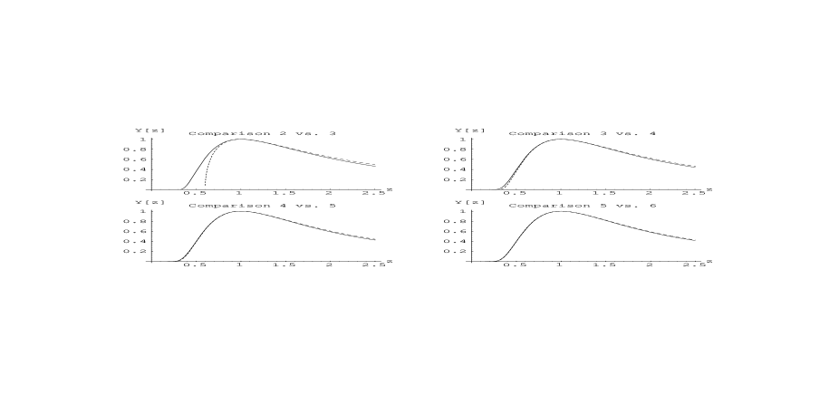
Figure 6: Illustration of the self-similarity property of the rescaled $l=1$ spectral densities. The plots show $Y_{1}^{(n)}(z)$ (dashed) compared with $Y_{1}^{(n+1)}(z)$ (solid) for $n=2,3,4,5$.

To substantiate proposal (b) let us prepare some further characteristics of the functions $R_{l}^{(n)}(x),\;l=0,1$: Its integral, its first, respectively minus first moment, and the strength of the asymptotic decay. In formulae

$$\begin{array}[]{ll}c_{0}^{(n)}={\displaystyle 12\pi\int_{0}^{\infty}dxR_{0}^{(n)}(x)}\makebox[56.9055pt]{ }&c_{1}^{(n)}={\displaystyle\int_{0}^{\infty}dxR^{(n)}_{1}(x)}\;,\\[6.45831pt] h^{(n)}_{0}={\displaystyle\int_{0}^{\infty}dx\,xR^{(n)}_{0}(x)}\;,&h^{(n)}_{1}={\displaystyle\int_{0}^{\infty}\frac{dx}{x}R^{(n)}_{1}(x)}\\[6.45831pt] R^{(n)}_{0}(x)\sim{\displaystyle\frac{A^{(n)}_{0}}{x^{4}}}\;,\;\;x\rightarrow\infty&R^{(n)}_{1}(x)\sim{\displaystyle\frac{A^{(n)}_{1}}{x^{2}}}\;,\;\;x\rightarrow\infty\;.\end{array}$$ (5.9)

In practice of course one will evaluate the constants $c^{(n)}_{l}$ and $h^{(n)}_{l}$ directly as $(n-1)$-fold unconstrained integrals, as in (3.31), rather than first computing the spectral densities and then evaluating their moments. For $n\leq 6$ the results for these constants are listed in Table 2.

Table 2: Integrals, $\pm$ first moments and decay constants

n	$\;\;\;\;c_{0}^{(n)}\;\;$	$\;\;10^{2}h^{(n)}_{0}\;\;$	$\;\;A^{(n)}_{0}\;\;$	$\;\;\;\;c_{1}^{(n)}\;\;$	$\;\;10h^{(n)}_{1}\;\;$	$\;\;A^{(n)}_{1}\;\;$
2	1.6027	8.231	0.727	1.009	3.958	1.938
3	0.4104	5.251	1.866	1.140	1.693	4.977
4	0.1943	4.140	3.308	1.242	1.054	8.821
5	0.1117	3.430	5.006	1.327	0.761	13.35
6	0.07185	2.930	6.938	1.400	0.594	18.50

In addition one has $c_{1}^{(1)}=\pi/4$. The decay constants $A_{l}^{(n)}$ are difficult to compute directly since the truly asymptotic behavior of the spectral densities sets in only at astronomically large energies $\mu\sim m\,e^{10\,n^{5/4}}$. Using the exact relations (3.32) they can however accurately be computed from the integrals $c_{1}^{(n)}$.

Making use of the convergence (5.4) one can deduce scaling laws for the quantities (5.9). To this end we introduce the corresponding quantities for the universal shape functions $Y_{l}(z)$

$$\begin{array}[]{ll}c_{0}^{*}={\displaystyle 12\pi\int_{0}^{\infty}dzY_{0}(z)\;,}\makebox[56.9055pt]{ }&c_{1}^{*}={\displaystyle\int_{0}^{\infty}dzY_{1}(z)}\;,\\[6.45831pt] h^{*}_{0}={\displaystyle\int_{0}^{\infty}dz\,zY_{0}(z)}\;,&h^{*}_{1}={\displaystyle\int_{0}^{\infty}\frac{dz}{z}Y_{1}(z)\;,}\\[6.45831pt] Y_{0}(z)\sim{\displaystyle\frac{A^{*}_{0}}{z^{4}}}\;,\;\;z\rightarrow\infty\;,&Y_{1}(z)\sim{\displaystyle\frac{A^{*}_{1}}{z^{2}}}\;,\;\;z\rightarrow\infty\;.\end{array}$$ (5.13)

For large enough $n$ we can approximate $R_{l}^{(n)}(x)$ pointwise and w.r.t. the moments by

$$R^{(n)}_{l}(x)\approx\frac{M_{l}}{n^{\gamma_{l}}}\;Y_{l}\left(\frac{x}{\xi_{l}n^{1+\alpha_{l}}}\right)\;.$$ (5.14)

Combining (5.5) - (5.14) one finds

$$\begin{array}[]{rclcrcl}c^{(n)}_{0}&\sim&c_{0}^{*}M_{0}\xi_{0}\;n^{1+\alpha_{0}-\gamma_{0}}\;,&\makebox[28.45274pt]{ }c^{(n)}_{1}&\sim&c_{1}^{*}M_{1}\xi_{1}\;n^{1+\alpha_{1}-\gamma_{1}}\;,\\[6.45831pt] h_{0}^{(n)}&\sim&h_{0}^{*}M_{0}\xi_{0}^{2}\;n^{2+2\alpha_{0}-\gamma_{0}}\;,&\makebox[28.45274pt]{ }h_{1}^{(n)}&\sim&h_{1}^{*}M_{1}\;n^{-\gamma_{1}}\;,\makebox[28.45274pt]{ }\\[6.45831pt] A_{0}^{(n)}&\sim&A_{0}^{*}M_{0}\xi_{0}^{4}\;n^{4+4\alpha_{0}-\gamma_{0}}\;,&\makebox[28.45274pt]{ }A_{1}^{(n)}&\sim&A_{1}^{*}M_{1}\xi_{1}^{2}\;n^{2+2\alpha_{1}-\gamma_{1}}\;.\end{array}$$ (5.18)

Two important constraints arise from the non-linear relations (3.32) for the asymptotic decay constants $A_{l}^{(n)}$. Combined with (5.18) this yields the following relations among the parameters

$$\gamma_{1}=1\;,\makebox[28.45274pt]{ } \frac{A_{1}^{*}}{(c_{1}^{*})^{2}M_{1}}=\pi\,\frac{\Gamma(\alpha_{1}+1)^{2}}{\Gamma(2\alpha_{1}+2)}\;,$$ (5.19)

$$\gamma_{0}=3+4\alpha_{0}-2\alpha_{1}\;,\makebox[28.45274pt]{ } \;A_{0}^{*}M_{0}\xi_{0}^{4}=\frac{3}{8}A_{1}^{*}M_{1}\xi_{1}^{2}\;.$$ (5.20)

(5.20b) follows trivially from $A_{1}^{(n)}=\frac{3}{8}A_{0}^{(n)}$. To arrive at (5.20a) we approximated

$$\sum_{k=1}^{n-1}[k(n-k)]^{\mu}\approx n^{2\mu+1}\int_{0}^{1}dy[y(1-y)]^{\mu}\;,$$

which is valid for large $n$. The exponents $\gamma_{l}$ are determined in terms of $\alpha_{0}$ and $\alpha_{1}$, which will later turn out coincide

$$\alpha_{0}=\alpha_{1}=:\alpha\;.$$ (5.22)

Re-inserting (5.20) and (5.22) into (5.18) one arrives at a simplified set of scaling relations. In particular

$$\frac{1}{h^{(n)}_{1}}\,\sim\,\frac{1}{h_{1}}\,n\;, h_{1}:=h_{1}^{*}M_{1}\;,$$

$$\frac{1}{h^{(n)}_{0}}\,\sim\,\frac{1}{h_{0}}\,n\;, h_{0}:=h_{0}^{*}M_{0}\xi_{0}^{2}\;,$$

$$[c_{0}^{(n)}]^{-1/(2+\alpha)}\,\sim\,c_{0}\,n\;, c_{0}:=(c_{0}^{*}M_{0}\xi_{0})^{-1/(2+\alpha)}\;,$$ (5.23)

are predicted to scale linearly with $n$. The same holds for the following two ratios, which provide a convenient way to determine the remaining exponent $\alpha$ from the slope of the linear function

$$\frac{A^{(n)}_{1}}{[c_{1}^{(n)}]^{2}}=\frac{8}{3}\,\frac{A^{(n)}_{0}}{[c_{1}^{(n)}]^{2}}\sim\pi\frac{\Gamma(\alpha+1)^{2}}{\Gamma(2\alpha+2)}\;n\;.$$ (5.24)

The predicted linear scaling in (5.23), (5.24) appears to be satisfied fairly well even for small $n=4,5,6$ as is illustrated in Figure 7.

Figure 7: Two-parameter linear fits for the $n$-dependence of various parameter combinations.

The fits are always two-parameter linear fits (slope and ordinate) on the largest three data points $n=4,5,6$. Using (5.24) the exponent $\alpha$ comes out to be

$$\alpha\approx 0.273\;.$$ (5.25)

Using this value in the fitting of $[c_{0}^{(n)}]^{-1/(2+\alpha)}$ the predicted linear scaling is confirmed. The quality of the $1/h^{(n)}_{0}$ fit confirms (5.22). For later use let us also note the values of the slopes in (5.23)

$$1/h_{1}=3.674\;,\;\;\;1/h_{0}=4.988\;,\;\;\;c_{0}=0.5643\;.$$ (5.26)

Similar fits can be made for the values and the positions of the maxima, given numerically in Table 1. They are similarly convincing; we refrain from displaying them.

5.2 Summation of $n$-particle contributions

Having at hand candidate expressions for the $n$-particle spectral densities as given in (5.14) one can evaluate their sum. Suppose that for $n<n_{0}$ the $n$-particle spectral densities have been computed explicitly; in our case $n_{0}=7$. Decomposing the sum

$$R_{l}(x)=\sum_{n=2-l}^{n_{0}-1}R_{l}^{(n)}(x)+\sum_{n=n_{0}}^{\infty}R_{l}^{(n)}(x)\;,$$ (5.27)

we wish to evaluate the second term. Using (5.14) the sum can be expressed in terms of a suitable integral transform of the shape function $Y_{l}(z)$. Here we shall need only the large $x$ asymptotics of the sum, in which case it is sufficient to approximate the sum over $n$ by an integral. One finds for the large $x$ behavior

$$\sum_{n=n_{0}}^{\infty}R_{l}^{(n)}(x)\ \longrightarrow\ \frac{M_{l}}{1+\alpha_{l}}\,\left(\frac{x}{\xi_{l}}\right)^{\frac{1-\gamma_{l}}{1+\alpha_{l}}}\;\int_{0}^{\infty}\frac{dz}{z}\;z^{\frac{\gamma_{l}-1}{1+\alpha_{l}}}\;Y_{l}(z)\;,\makebox[28.45274pt]{ }x\rightarrow\infty\;,$$ (5.28)

where the corrections are at least one power down in $x$. Clearly the physical spectral densities can be evaluated similarly; summing only over odd/even particle numbers will simply result in an extra factor $1/2$ in the asymptotic expression (5.28). In particular in the isospin $1$ case the exponent $\gamma_{1}=1$ yields the asymptotics $R_{1}(x)\rightarrow A_{1}$. One can show that the asymptotics of $R_{0}(x)$ must always be down by two orders in $x$, compared to that of $R_{1}(x)$. This is related to, although not a direct consequence of (3.30). One concludes that the $x\rightarrow\infty$ asymptotics in the isospin zero case must be $R_{0}(x)\rightarrow A_{0}/x^{2}$. Comparing with (5.28) this requires $\alpha_{0}=\alpha_{1}$, as claimed before. Moreover one obtains the relations

$$A^{\rm curr} = \frac{\pi}{4}A^{\rm spin}=\frac{h_{1}}{2(1+\alpha)}\;,$$ (5.29)

$$A^{\rm EM} = 4A^{\rm top}=\frac{h_{0}}{2(1+\alpha)}\;,$$ (5.30)

which have various interesting consequences. (5.30a) relates $A^{\rm curr}$ to $A^{\rm spin}$. This is interesting because $A^{\rm curr}$ is accessible to perturbation theory, while $A^{\rm spin}$ is some previously unknown non-perturbative constant, which via (2.44), (2.46) determines the short-distance normalization of the Spin two-point function. On the other hand both constants also get expressed in terms of the scaling hypothesis. Using (5.25) and (5.26) one finds $(A^{\rm curr})_{SH}=1/9.3553=1.007/3\pi$. Since perturbation theory gives $(A^{\rm curr})_{PT}=1/3\pi$ one sees that not only the functional form of the asymptotic behavior obtained from the resummation of the spectral resolution agrees with that predicted by PT, but also the numerical value of the leading coefficient agrees with an accuracy better than $1\%$. Depending on the viewpoint one can interpret this as supporting the validity of PT and/or our scaling hypothesis . Accepting the PT value for $A^{\rm curr}$ we get the exact prediction for the non-perturbative constant $\lambda_{1}=A^{\rm spin}$ anticipated in (2.47)

$$\lambda_{1}=A^{\rm spin}=\frac{4}{3\pi^{2}}=0.135095\;.$$ (5.32)

On the other hand $A^{\rm spin}$ has been evaluated by Monte Carlo simulations [15] with the result $(A^{\rm spin})_{MC}=0.135(2)$, convincingly close to the proposed exact result. The similar behavior of the Spin and Current two-point functions and spectral densities for large energy is again an O$(3)$ speciality, as can be seen from (2.48).

A similar pattern underlies (5.30b). Now both $A^{\rm EM}$ and $A^{\rm top}$ can be computed in PT. The results are given in (2.69), (2.75) and yield in particular $(A^{\rm EM})_{PT}=4(A^{\rm top})_{PT}$. The non-perturbative result now is that this transfers to relations for the exact spectral densities at all energy scales

$$\rho^{\rm EM}(\mu)=\sum_{k=1}^{\infty}\rho_{0}^{(2k)}(\mu)\,,\makebox[28.45274pt]{ }\rho^{\rm top}(\mu)=\frac{1}{4}\sum_{k=1}^{\infty}\rho_{0}^{(2k+1)}(\mu)\;,$$ (5.33)

which is the announced result (2.62). Consistency then requires that the numerical value for $A^{EM}$ computed via the scaling hypothesis coincides with the perturbative value. Combining (5.25), (5.26) and (2.75) one finds

$$(A^{\rm EM})_{SH}=1/12.700=0.989/4\pi\;,\makebox[28.45274pt]{ }(A^{\rm EM})_{PT}=1/4\pi\;.$$ (5.34)

Note that here the matching between full and perturbative dynamics already concerns a 1-loop coefficient and is accurate to $1\%$. Again this cuts both ways, supporting the validity of PT and/or our scaling hypothesis and thus also the proposed normalization constant $\lambda_{0}=1/4$ of the topological charge density operator.

Finally consider the central charge as defined in (2.19). In the spectral resolution it again decomposes into a sum of $n$-particle contribution. The first few terms are given in Table 2, i.e.

$$c^{(2)}_{0}=1.603\;,\;\;c^{(4)}_{0}=0.194\;,\;\;c^{(6)}_{0}=0.072\;,\makebox[28.45274pt]{ }c^{(n)}_{0}=12\pi\int_{0}^{\infty}d\mu\,\rho^{(n)}_{0}(\mu)\;.$$ (5.35)

The remainder of the series can be evaluated by means of the scaling hypothesis. Using (5.26), (5.25) one finds

$$c_{SH}=c^{(2)}_{0}+c^{(4)}_{0}+c^{(6)}_{0}+\sum_{k=4}^{\infty}(2kc_{0}-0.200)^{-(2+\alpha)}=1.997\;.$$ (5.36)

Here we also used the ordinate of the linear fit. (Tree level) PT predicts $c_{PT}=2$, corresponding to the two unconstrained bosonic degrees of freedom. The form factor computation shows that this is compatible with the non-perturbative low energy dynamics of the model and provides further support for the scaling hypothesis (see the footnote on page 38). An alternative non-perturbative consistency check is provided by the thermodynamic Bethe Ansatz [38] and also yields $c=2$. Let us point out that the value $c=2$ does not carry much information about the nature of the UV limiting CFT. For a number of reasons it cannot be the Gaussian $c=2$ model.

5.3 Towards the exact two-point functions

The scaling hypothesis also allows one to numerically compute the two-point functions at all energy/length scales. In coordinate space this simply amounts to performing the integral in the spectral representation, once the full spectral density is available via (5.27) and (5.14). In momentum space one can combine eq. (2.11) and (5.14) to evaluate the sum over all $n$-particle contributions to the functions $I(p)$, basically giving the Fourier transform of the two-point function. The results will be described in [39].

6. Conclusions

In this paper we studied the two-point functions of the four physically most interesting operators in the O$(3)$ NLS model. We have chosen the O$(3)$ model because it is the simplest 2-dimensional theory that resembles in many aspects QCD. Concerning the on-shell features various exact results, in particular the exact two-particle S-matrix are known [25, 24], due to its remarkable integrability properties. On the other hand there exist a large number of MC studies of the model [27, 22, 35, 15, 36], not making use of this integrability. Here we employed the form factor bootstrap method for integrable QFTs to compute off-shell features that can be compared both with PT and with MC data. A simplifying feature of the O$(3)$ model (as compared, say, to the higher O$(N)$ models) is that the computation of the form factors is relatively straightforward due to their essentially polynomial nature. Once the form factors are known, the two-point functions can be evaluated in terms of a spectral resolution; that is as an infinite sum where multiple integrals of the squares of the $n$-particle form factors enter, the sum running over all particle numbers $n$. In practice one has to truncate this infinite sum after the first few terms. In models with a diagonal S-matrix and a power-like approach of the UV limit, application of this technique showed extremely fast convergence of the truncated sum [10, 11, 12]. In an asymptotically free theory one expects less fast convergence, because the approach to the asymptotic form is only logarithmic. Thus, in order to really check the validity of PT (which has been questioned [3, 4]) we needed to extrapolate our results beyond the largest particle number, presently 6, for which we carried out the computations explicitly. The extrapolation was based on a novel scaling hypothesis. Using this hypothesis we have been able to compute the extreme UV properties independent of PT. Remarkably we found very good agreement with PT: Within 1% for a RG improved tree level coefficient in the case of the Current and also within 1% for a RG improved 1-loop coefficient in the case of the EM tensor. This is very strong evidence for PT. The agreement between our extrapolated data and PT also indirectly confirms the proposed exact value of the perturbative $\Lambda$ parameter [16]. On the basis of the evidence presented in section 5 we regard this scaling hypothesis as very plausible, although an analytical proof remains to be found and would be highly desirable. On the other hand, the nature of this hypothesis is completely independent of the assumptions underlying the derivation of the usual RG improved expressions based on PT, so that the agreement of the results is still remarkable.

A further result is the exact determination of two, previously unknown, non-perturbative constants $\lambda_{0}$ and $\lambda_{1}$. Using the values of these numbers, we can write the exact 3-particle matrix element of the properly normalized topological charge density operator $q(x)$ as

$$\langle 0|\,q(0)\,|a_{3},{\theta}_{3};a_{2},{\theta}_{2};a_{1},{\theta}_{1}\rangle=\frac{\pi^{\frac{7}{2}}}{4}\,\Big{[}m^{2}-M^{(3)}({\theta}_{3},{\theta}_{2},{\theta}_{1})^{2}\Big{]}\,\Psi({\theta}_{3},{\theta}_{2},{\theta}_{1})\,\epsilon^{a_{3}a_{2}a_{1}}\,,$$ (6.1)

where $M^{(3)}({\theta}_{3},{\theta}_{2},{\theta}_{1})$ is the three-particle invariant mass. Further the short distance expansion of the Spin two-point function is now unambiguously fixed to be

$$S^{\rm spin}(x)=\frac{1}{3\pi^{3}}\left(\ln mr\right)^{2}+O\left(\ln\ln mr\cdot\ln mr\right)\,,$$ (6.2)

where $m$ is the mass gap and $r=\sqrt{x_{1}^{2}+x_{2}^{2}}$. Note that the values of the overall constants in (6.1) and (6.2) follow from the scaling hypothesis alone, we do not need here the results of any numerical fitting procedure.

Finally we remark that our scaling hypothesis may be viewed as a 2-dimensional analogue of the KNO scaling [40] in QCD. We also expect that scaling hypotheses of a similar type can be formulated in many other 2-dimensional models, giving simultaneous access to their off-shell properties at all energy/length scales.

Acknowledgements: We wish to thank H. Lehmann, F. Niedermayer, A. Patrascioiu, E. Seiler and P. Weisz for stimulating discussions. In particular we thank E. Seiler for initially suggesting to study the $n$-dependence of the spectral densities with hindsight to extrapolations. A.P. and E.S. we thank in addition for generously allowing us to use their data prior to publication. M.N. acknowledges support by the Reimar Lüst fellowship of the Max-Planck-Society. J.B. wishes to thank the Theory Group at MPI Munich for their hospitality.

Appendix: List of form factor squares

Here we list the results for the form factor squares for the EM tensor & TC density and Current & Spin series up to 6 particles. The corresponding Mathematica files can be obtained from the authors upon request. The squares are boost invariant symmetric polynomials in the rapidities and therefore conveniently described in terms of a basis in this space of polynomials.

Let $P^{(n)}(N,p)$ denote the space of homogeneous symmetric polynomials in $n$ variables that are of total degree $N$ and partial degree $p$. By partial degree we mean the power with which an individual variable enters. A basis for $P^{(n)}(N,p)$ can be obtained as follows. For fixed $n$ let $\sigma_{1}^{(n)},\ldots,\sigma_{n}^{(n)}$ denote the elementary symmetric polynomials in ${\theta}_{1},\ldots,{\theta}_{n}$, i.e.

$$\sigma_{k}^{(n)}=\sum_{i_{1}<\ldots<i_{k}}{\theta}_{i_{1}}\ldots{\theta}_{i_{k}}\;.$$ (A.3)

Let $\lambda=(\lambda_{1},\ldots,\lambda_{p}),\;\lambda_{1}\leq\lambda_{2}\leq\ldots\leq\lambda_{p}$ be a partition of $N$ into $p$ parts less or equal to $n$, i.e. $\sum_{i}\lambda_{i}=N,\;1\leq\lambda_{i}\leq n,\;1\leq i\leq p$. Running through all those partitions, the assignment

$$(\lambda_{1},\ldots,\lambda_{p})\ \longrightarrow\ \sigma^{(n)}_{\lambda_{1}}\ldots\sigma^{(n)}_{\lambda_{p}}$$

provides a basis of $P^{(n)}(N,p)$. However these functions are not boost invariant and one would like to have a description of the boost invariant subspace $P_{inv}^{(n)}(N,p)$ of $P^{(n)}(N,p)$. Boost invariance can be incorporated by switching to symmetric polynomials $\tau^{(n)}_{k}$ defined by

$$\tau^{(n)}_{k}({\theta}_{1},\ldots,{\theta}_{n})=\sigma^{(n)}_{k}(\widehat{{\theta}}_{1},\ldots,\widehat{{\theta}}_{n})\;,\makebox[28.45274pt]{ }2\leq k\leq n\;,$$

$$\tau^{(n)}_{1}=\frac{1}{n}\sigma^{(n)}_{1}\;,\makebox[28.45274pt]{ }\widehat{{\theta}}_{j}={\theta}_{j}-\frac{1}{n}({\theta}_{1}+\ldots+{\theta}_{n})\;.$$ (A.4)

All monomials in the $\tau^{(n)}_{k}$’s ($k\geq 2)$ are manifestly boost invariant. The price to pay is that the partial degree is no longer manifest. For a monomial in the $\sigma^{(n)}_{k}$’s the partial degree is simply given by the number of $\sigma^{(n)}_{k}$ factors. This is no longer the case for monomials in the $\tau^{(n)}_{k}$’s. In fact, inverting the relation

$$\sigma_{k}={n\choose k}\,\tau_{1}^{k}+\sum_{j=2}^{k}{n-j\choose k-j}\;\tau_{1}^{k-j}\,\tau_{j}\;,\makebox[28.45274pt]{ }k=1,\ldots,n$$ (A.5)

(here and henceforth the superscripts $(n)$ are suppressed) one sees that $\tau_{k}=(-\sigma_{1})^{k}{n\choose k}(1-k)n^{-k}+\ldots+\sigma_{k}$. Thus for a monomial in the $\tau_{k}$’s the total and the partial degree coincide. Linear combinations of such monomials however may have a partial degree that is less than their total degree.

The general structure of the polynomials $G^{(n)}_{l}({\theta})$ can now be described as follows.

$$G^{(n)}_{l}({\theta})=G^{(n)}_{l;0}({\theta})+\pi^{2}G^{(n)}_{l;2}({\theta})+\ldots+\pi^{N}G^{(n)}_{l;N}({\theta})\;,\;\;\;G^{(n)}_{l;2k}({\theta})\in P_{inv}^{(n)}(N-2k,p)\;.$$ (A.6)

The overall leading terms $G^{(n)}_{l;0}({\theta})$ are given in (3.26). Below we list the results for the polynomials $G^{(n)}_{l}({\theta}),\;n\leq 6$ for the Spin & Current and EM tensor & TC density series:

Spin & Current

$$G_{1}^{(1)}({\theta})=1\;,\makebox[28.45274pt]{ }G_{1}^{(2)}({\theta})=2\;,\makebox[28.45274pt]{ }G_{1}^{(3)}({\theta})=12[-\tau_{2}+\pi^{2}]\;,$$

$$G_{1}^{(4)}({\theta})=-4[6\tau_{2}^{3}+9\tau_{3}^{2}+40\tau_{2}\tau_{4}]+8\pi^{2}[25\tau_{2}^{2}+44\tau_{4}]-448\pi^{4}\tau_{2}+272\pi^{6}\;,$$

$$G_{1}^{(5)}({\theta})=[-48\tau_{2}^{3}\tau_{3}^{2}-72\tau_{3}^{4}+144\tau_{2}^{4}\tau_{4}+52\tau_{2}\tau_{3}^{2}\tau_{4}+352\tau_{2}^{2}\tau_{4}^{2}-640\tau_{4}^{3}+$$

$$+660\tau_{2}^{2}\tau_{3}\tau_{5}+3200\tau_{3}\tau_{4}\tau_{5}+4500\tau_{2}\tau_{5}^{2}]$$

$$-4\pi^{2}[36\tau_{2}^{5}-64\tau_{2}^{2}\tau_{3}^{2}+692\tau_{2}^{3}\tau_{4}+295\tau_{3}^{2}\tau_{4}+80\tau_{2}\tau_{4}^{2}+2925\tau_{2}\tau_{3}\tau_{5}+4375\tau_{5}^{2}]$$

$$+16\pi^{4}[160\tau_{2}^{4}+97\tau_{2}\tau_{3}^{2}+909\tau_{2}^{2}\tau_{4}-20\tau_{4}^{2}+1950\tau_{3}\tau_{5}]$$

$$-16\pi^{6}[978\tau_{2}^{3}+380\tau_{3}^{2}+1965\tau_{2}\tau_{4}]$$

$$+64\pi^{8}[678\tau_{2}^{2}+395\tau_{4}]-55120\,\pi^{10}\tau_{2}+24960\,\pi^{12}\;,$$

$$G_{1}^{(6)}({\theta})=4[-24\tau_{2}^{3}\tau_{3}^{2}\tau_{4}^{2}-36\tau_{3}^{4}\tau_{4}^{2}+72\tau_{2}^{4}\tau_{4}^{3}+26\tau_{2}\tau_{3}^{2}\tau_{4}^{3}+176\tau_{2}^{2}\tau_{4}^{4}-320\tau_{4}^{5}$$

$$+72\tau_{2}^{3}\tau_{3}^{3}\tau_{5}+108\tau_{3}^{5}\tau_{5}-228\tau_{2}^{4}\tau_{3}\tau_{4}\tau_{5}-57\tau_{2}\tau_{3}^{3}\tau_{4}\tau_{5}-446\tau_{2}^{2}\tau_{3}\tau_{4}^{2}\tau_{5}+2208\tau_{3}\tau_{4}^{3}\tau_{5}$$

$$+108\tau_{2}^{5}\tau_{5}^{2}-801\tau_{2}^{2}\tau_{3}^{2}\tau_{5}^{2}+1182\tau_{2}^{3}\tau_{4}\tau_{5}^{2}-3615\tau_{3}^{2}\tau_{4}\tau_{5}^{2}-430\tau_{2}\tau_{4}^{2}\tau_{5}^{2}+1800\tau_{2}\tau_{3}\tau_{5}^{3}$$

$$+5625\tau_{5}^{4}-180\tau_{2}^{4}\tau_{3}^{2}\tau_{6}-621\tau_{2}\tau_{3}^{4}\tau_{6}+480\tau_{2}^{5}\tau_{4}\tau_{6}+2082\tau_{2}^{2}\tau_{3}^{2}\tau_{4}\tau_{6}-2344\tau_{2}^{3}\tau_{4}^{2}\tau_{6}$$

$$-1710\tau_{3}^{2}\tau_{4}^{2}\tau_{6}-128\tau_{2}\tau_{4}^{3}\tau_{6}+3204\tau_{2}^{3}\tau_{3}\tau_{5}\tau_{6}+3753\tau_{3}^{3}\tau_{5}\tau_{6}-744\tau_{2}\tau_{3}\tau_{4}\tau_{5}\tau_{6}$$

$$+14490\tau_{2}^{2}\tau_{5}^{2}\tau_{6}-34950\tau_{4}\tau_{5}^{2}\tau_{6}-288\tau_{2}^{4}\tau_{6}^{2}+13230\tau_{2}\tau_{3}^{2}\tau_{6}^{2}-18696\tau_{2}^{2}\tau_{4}\tau_{6}^{2}$$

$$+40464\tau_{4}^{2}\tau_{6}^{2}+48870\tau_{3}\tau_{5}\tau_{6}^{2}+61992\tau_{2}\tau_{6}^{3}]$$

$$-4\pi^{2}[72\tau_{2}^{3}\tau_{3}^{4}+108\tau_{3}^{6}-384\tau_{2}^{4}\tau_{3}^{2}\tau_{4}-408\tau_{2}\tau_{3}^{4}\tau_{4}+600\tau_{2}^{5}\tau_{4}^{2}+26\tau_{2}^{2}\tau_{3}^{2}\tau_{4}^{2}$$

$$+2248\tau_{2}^{3}\tau_{4}^{3}+1846\tau_{3}^{2}\tau_{4}^{3}-1504\tau_{2}\tau_{4}^{4}-264\tau_{2}^{5}\tau_{3}\tau_{5}-582\tau_{2}^{2}\tau_{3}^{3}\tau_{5}-3518\tau_{2}^{3}\tau_{3}\tau_{4}\tau_{5}$$

$$-6525\tau_{3}^{3}\tau_{4}\tau_{5}+8258\tau_{2}\tau_{3}\tau_{4}^{2}\tau_{5}+5574\tau_{2}^{4}\tau_{5}^{2}-11685\tau_{2}\tau_{3}^{2}\tau_{5}^{2}+22220\tau_{2}^{2}\tau_{4}\tau_{5}^{2}$$

$$-14450\tau_{4}^{2}\tau_{5}^{2}+32625\tau_{3}\tau_{5}^{3}+1056\tau_{2}^{6}\tau_{6}+4110\tau_{2}^{3}\tau_{3}^{2}\tau_{6}+891\tau_{3}^{4}\tau_{6}+2768\tau_{2}^{4}\tau_{4}\tau_{6}$$

$$+23766\tau_{2}\tau_{3}^{2}\tau_{4}\tau_{6}-54496\tau_{2}^{2}\tau_{4}^{2}\tau_{6}+30848\tau_{4}^{3}\tau_{6}+86190\tau_{2}^{2}\tau_{3}\tau_{5}\tau_{6}-54090\tau_{3}\tau_{4}\tau_{5}\tau_{6}$$

$$+78600\tau_{2}\tau_{5}^{2}\tau_{6}-47688\tau_{2}^{3}\tau_{6}^{2}+136404\tau_{3}^{2}\tau_{6}^{2}+51432\tau_{2}\tau_{4}\tau_{6}^{2}+378000\tau_{6}^{3}]$$

$$+16\pi^{4}[-126\tau_{2}^{5}\tau_{3}^{2}-24\tau_{2}^{2}\tau_{3}^{4}+336\tau_{2}^{6}\tau_{4}-1272\tau_{2}^{3}\tau_{3}^{2}\tau_{4}-1020\tau_{3}^{4}\tau_{4}+3818\tau_{2}^{4}\tau_{4}^{2}$$

$$+3769\tau_{2}\tau_{3}^{2}\tau_{4}^{2}+426\tau_{2}^{2}\tau_{4}^{3}+376\tau_{4}^{4}-612\tau_{2}^{4}\tau_{3}\tau_{5}-6291\tau_{2}\tau_{3}^{3}\tau_{5}+6302\tau_{2}^{2}\tau_{3}\tau_{4}\tau_{5}$$

$$+876\tau_{3}\tau_{4}^{2}\tau_{5}+21468\tau_{2}^{3}\tau_{5}^{2}-135\tau_{3}^{2}\tau_{5}^{2}+23185\tau_{2}\tau_{4}\tau_{5}^{2}+5640\tau_{2}^{5}\tau_{6}+29352\tau_{2}^{2}\tau_{3}^{2}\tau_{6}$$

$$-29108\tau_{2}^{3}\tau_{4}\tau_{6}+19149\tau_{3}^{2}\tau_{4}\tau_{6}-41452\tau_{2}\tau_{4}^{2}\tau_{6}+142074\tau_{2}\tau_{3}\tau_{5}\tau_{6}+33075\tau_{5}^{2}\tau_{6}$$

$$-93966\tau_{2}^{2}\tau_{6}^{2}+159882\tau_{4}\tau_{6}^{2}]$$

$$-8\pi^{6}[408\tau_{2}^{7}-4482\tau_{2}^{4}\tau_{3}^{2}-6564\tau_{2}\tau_{3}^{4}+18276\tau_{2}^{5}\tau_{4}+10016\tau_{2}^{2}\tau_{3}^{2}\tau_{4}+45484\tau_{2}^{3}\tau_{4}^{2}$$

$$+20301\tau_{3}^{2}\tau_{4}^{2}-5116\tau_{2}\tau_{4}^{3}+24628\tau_{2}^{3}\tau_{3}\tau_{5}-37755\tau_{3}^{3}\tau_{5}+117453\tau_{2}\tau_{3}\tau_{4}\tau_{5}+264035\tau_{2}^{2}\tau_{5}^{2}$$

$$+72675\tau_{4}\tau_{5}^{2}+69236\tau_{2}^{4}\tau_{6}+381147\tau_{2}\tau_{3}^{2}\tau_{6}-507872\tau_{2}^{2}\tau_{4}\tau_{6}-17628\tau_{4}^{2}\tau_{6}$$

$$+623655\tau_{3}\tau_{5}\tau_{6}-418404\tau_{2}\tau_{6}^{2}]$$

$$+32\pi^{8}[2964\tau_{2}^{6}-3444\tau_{2}^{3}\tau_{3}^{2}-6138\tau_{3}^{4}+40900\tau_{2}^{4}\tau_{4}+30984\tau_{2}\tau_{3}^{2}\tau_{4}+26211\tau_{2}^{2}\tau_{4}^{2}$$

$$-1048\tau_{4}^{3}+69483\tau_{2}^{2}\tau_{3}\tau_{5}+62973\tau_{3}\tau_{4}\tau_{5}+181365\tau_{2}\tau_{5}^{2}+33996\tau_{2}^{3}\tau_{6}$$

$$+182187\tau_{3}^{2}\tau_{6}-353994\tau_{2}\tau_{4}\tau_{6}-129717\tau_{6}^{2}]$$

$$-32\pi^{10}[31348\tau_{2}^{5}+14205\tau_{2}^{2}\tau_{3}^{2}+177930\tau_{2}^{3}\tau_{4}+60772\tau_{3}^{2}\tau_{4}$$

$$+18686\tau_{2}\tau_{4}^{2}+237656\tau_{2}\tau_{3}\tau_{5}+184975\tau_{5}^{2}-6386\tau_{2}^{2}\tau_{6}-357082\tau_{4}\tau_{6}]$$

$$+32\pi^{12}[168412\tau_{2}^{4}+78879\tau_{2}\tau_{3}^{2}+418856\tau_{2}^{2}\tau_{4}-8772\tau_{4}^{2}+260811\tau_{3}\tau_{5}-56784\tau_{2}\tau_{6}]$$

$$-16\pi^{14}[1020460\tau_{2}^{3}+177855\tau_{3}^{2}+1047914\tau_{2}\tau_{4}+19362\tau_{6}]$$

$$+128\pi^{16}[220109\tau_{2}^{2}+70513\tau_{4}]-25589760\,\pi^{18}\tau_{2}+9265536\,\pi^{20}\;.$$

EM tensor & TC density:

$$G_{0}^{(2)}({\theta})=\frac{1}{\pi^{2}-4\tau_{2}}\;,\makebox[28.45274pt]{ }G_{0}^{(3)}({\theta})=2$$

$$G_{0}^{(4)}({\theta})=4[12\tau_{4}+\tau_{2}^{2}]-\pi^{2}32\tau_{2}+28\,\pi^{4}\;,$$

$$G_{0}^{(5)}({\theta})=4[2\tau_{2}^{2}\tau_{3}^{2}-6\tau_{2}^{3}\tau_{4}+15\tau_{3}^{2}\tau_{4}-40\tau_{2}\tau_{4}^{2}-25\tau_{2}\tau_{3}\tau_{5}-625\tau_{5}^{2}]$$

$$+8\pi^{2}[3\tau_{2}^{4}-11\tau_{2}\tau_{3}^{2}+73\tau_{2}^{2}\tau_{4}+60\tau_{4}^{2}+275\tau_{3}\tau_{5}]-56\pi^{4}[8\tau_{2}^{3}+5\tau_{3}^{2}+40\tau_{2}\tau_{4}]$$

$$+8\pi^{6}[253\tau_{2}^{2}+270\tau_{4}]-3280\pi^{8}\tau_{2}+1680\,\pi^{10}\;,$$

$$G_{0}^{(6)}({\theta})=4[4\tau_{2}^{2}\tau_{3}^{2}\tau_{4}^{2}-12\tau_{2}^{3}\tau_{4}^{3}+30\tau_{3}^{2}\tau_{4}^{3}-80\tau_{2}\tau_{4}^{4}-12\tau_{2}^{2}\tau_{3}^{3}\tau_{5}+38\tau_{2}^{3}\tau_{3}\tau_{4}\tau_{5}$$

$$-99\tau_{3}^{3}\tau_{4}\tau_{5}+246\tau_{2}\tau_{3}\tau_{4}^{2}\tau_{5}-18\tau_{2}^{4}\tau_{5}^{2}+165\tau_{2}\tau_{3}^{2}\tau_{5}^{2}-320\tau_{2}^{2}\tau_{4}\tau_{5}^{2}-450\tau_{4}^{2}\tau_{5}^{2}$$

$$+1125\tau_{3}\tau_{5}^{3}+30\tau_{2}^{3}\tau_{3}^{2}\tau_{6}+81\tau_{3}^{4}\tau_{6}-80\tau_{2}^{4}\tau_{4}\tau_{6}-234\tau_{2}\tau_{3}^{2}\tau_{4}\tau_{6}+212\tau_{2}^{2}\tau_{4}^{2}\tau_{6}$$

$$-48\tau_{4}^{3}\tau_{6}-438\tau_{2}^{2}\tau_{3}\tau_{5}\tau_{6}+1530\tau_{3}\tau_{4}\tau_{5}\tau_{6}-9300\tau_{2}\tau_{5}^{2}\tau_{6}-48\tau_{2}^{3}\tau_{6}^{2}-5022\tau_{3}^{2}\tau_{6}^{2}$$

$$+10332\tau_{2}\tau_{4}\tau_{6}^{2}-59940\tau_{6}^{3}]$$

$$+8\pi^{2}[6\tau_{2}^{2}\tau_{3}^{4}-32\tau_{2}^{3}\tau_{3}^{2}\tau_{4}+36\tau_{3}^{4}\tau_{4}+50\tau_{2}^{4}\tau_{4}^{2}-197\tau_{2}\tau_{3}^{2}\tau_{4}^{2}+394\tau_{2}^{2}\tau_{4}^{3}+216\tau_{4}^{4}$$

$$-22\tau_{2}^{4}\tau_{3}\tau_{5}+3\tau_{2}\tau_{3}^{3}\tau_{5}-448\tau_{2}^{2}\tau_{3}\tau_{4}\tau_{5}-390\tau_{3}\tau_{4}^{2}\tau_{5}+550\tau_{2}^{3}\tau_{5}^{2}-2325\tau_{3}^{2}\tau_{5}^{2}$$

$$+4225\tau_{2}\tau_{4}\tau_{5}^{2}+88\tau_{2}^{5}\tau_{6}+246\tau_{2}^{2}\tau_{3}^{2}\tau_{6}+444\tau_{2}^{3}\tau_{4}\tau_{6}+1683\tau_{3}^{2}\tau_{4}\tau_{6}-5020\tau_{2}\tau_{4}^{2}\tau_{6}$$

$$+11220\tau_{2}\tau_{3}\tau_{5}\tau_{6}+22125\tau_{5}^{2}\tau_{6}-10854\tau_{2}^{2}\tau_{6}^{2}+8730\tau_{4}\tau_{6}^{2}]$$

$$+8\pi^{4}[42\tau_{2}^{4}\tau_{3}^{2}-72\tau_{2}\tau_{3}^{4}-112\tau_{2}^{5}\tau_{4}+832\tau_{2}^{2}\tau_{3}^{2}\tau_{4}-1804\tau_{2}^{3}\tau_{4}^{2}+179\tau_{3}^{2}\tau_{4}^{2}$$

$$-1696\tau_{2}\tau_{4}^{3}+236\tau_{2}^{3}\tau_{3}\tau_{5}+2943\tau_{3}^{3}\tau_{5}-3809\tau_{2}\tau_{3}\tau_{4}\tau_{5}-8435\tau_{2}^{2}\tau_{5}^{2}$$

$$-13075\tau_{4}\tau_{5}^{2}-1952\tau_{2}^{4}\tau_{6}-10899\tau_{2}\tau_{3}^{2}\tau_{6}+13288\tau_{2}^{2}\tau_{4}\tau_{6}+5008\tau_{4}^{2}\tau_{6}$$

$$-46035\tau_{3}\tau_{5}\tau_{6}+38916\tau_{2}\tau_{6}^{2}]$$

$$+16\pi^{6}[34\tau_{2}^{6}-480\tau_{2}^{3}\tau_{3}^{2}-597\tau_{3}^{4}+1790\tau_{2}^{4}\tau_{4}+424\tau_{2}\tau_{3}^{2}\tau_{4}+4665\tau_{2}^{2}\tau_{4}^{2}+1182\tau_{4}^{3}+$$

$$3281\tau_{2}^{2}\tau_{3}\tau_{5}+9435\tau_{3}\tau_{4}\tau_{5}+17425\tau_{2}\tau_{5}^{2}+2692\tau_{2}^{3}\tau_{6}+17979\tau_{3}^{2}\tau_{6}$$

$$-29530\tau_{2}\tau_{4}\tau_{6}-25185\tau_{6}^{2}]$$

$$+32\pi^{8}[-540\tau_{2}^{5}+291\tau_{2}^{2}\tau_{3}^{2}-6338\tau_{2}^{3}\tau_{4}-2488\tau_{3}^{2}\tau_{4}-4222\tau_{2}\tau_{4}^{2}-9908\tau_{2}\tau_{3}\tau_{5}$$

$$-9775\tau_{5}^{2}+698\tau_{2}^{2}\tau_{6}+18322\tau_{4}\tau_{6}]$$

$$+64\pi^{10}[2308\tau_{2}^{4}+1170\tau_{2}\tau_{3}^{2}+9556\tau_{2}^{2}\tau_{4}+1012\tau_{4}^{2}+6345\tau_{3}\tau_{5}-1980\tau_{2}\tau_{6}]$$

$$-16\pi^{12}[35992\tau_{2}^{3}+7683\tau_{3}^{2}+53924\tau_{2}\tau_{4}+372\tau_{6}]$$

$$+32\pi^{14}[36053\tau_{2}^{2}+15241\tau_{4}]-1148928\,\pi^{16}\tau_{2}+440128\,\pi^{18}\;.$$

References

• [1] E. Brezin, J. Zinn-Justin and J.C. Le Guillon, Phys. Rev. D14 (1976) 2615.
• [2] A. Polyakov, Phys. Lett. B59 (1975) 79.
E. Brezin and J. Zinn-Justin, Phys. Rev. B14 (1976) 3110.
W.A. Bardeen, B.W. Lee and R.E. Shrock, Phys. Rev. D14 (1976) 985.
• [3] A. Patrascioiu and E. Seiler, “Two dimensional NLS Models: Orthodoxy and Heresy”, in Fields and Particles, Schladming 1990, ed. H. Mitter and W. Schweiger.
“The Difference between Abelian and Non-Abelian Models: Fact and Fancy”, MPI-Ph 91-88.
A. Patrascioiu and E. Seiler, Phys. Rev. Lett 74 (1995) 1924.
• [4] A. Patrascioiu and E. Seiler, Phys. Rev. Lett 74 (1995) 1920.
• [5] F. David, Comm. Math. Phys. 81 (1981) 149.
S. Elitzur, Nucl. Phys. B212 (1983) 501.
• [6] F. David, Phys. Rev. Lett. 75 (1995) 2626.
A. Patrascioiu and E. Seiler, Phys. Rev. Lett 75 (1995) 2627.
F. Niedermayer, M. Niedermaier and P. Weisz, MPI-Ph/96-121.
• [7] J. Balog and M. Niedermaier, ‘Exact form factors in the O(3) NLS model’, in preparation
• [8] M. Karowski and P. Weisz, Nucl. Phys. B139 (1978) 455.
• [9] F.A. Smirnov, ‘Form Factors in Completely Integrable Models of Quantum Field Theory’, World Scientific, 1992.
• [10] V. Yurov and Al. B. Zamolodchikov, Int. J. Mod. Phys A6 (1991) 3419.
• [11] A. Fring, G. Mussardo and P. Simonetti, Nucl. Phys. B393 (1993) 413.
J. Cardy and G. Mussardo, Nucl. Phys. B410 (1993) 451.
G. Delfino and G. Mussardo, Phys. Lett. B324 (1994) 40; Nucl. Phys. B455 (1995) 724.
C. Acerbi, G. Mussardo and A. Valleriani, hep-th/9601113
• [12] H. Lesage, H. Saleur and S. Skorik, Nucl. Phys. B474 (1996) 602.
• [13] G. Källèn, Dan. mat. fys. Medd. 27 (1953) 1.
H. Lehmann, Nuovo Cim. 11 (1954) 342.
• [14] J. Balog, M. Niedermaier and T. Hauer, Phys. Lett. B386 (1996) 224.
• [15] A. Patrascioiu and E. Seiler, to be published
• [16] P. Hasenfratz, M. Maggiore and F. Niedermayer, Phys. Lett. B245 (1990) 522.
P. Hasenfratz and F. Niedermayer, Phys. Lett. B245 (1990) 529.
• [17] W. Magnus, F. Oberhettinger and R. Soni, ‘Special Functions’, Springer, 1966
• [18] A. Zamolodchikov, JETP Lett. 43 (1986) 730.
• [19] A. Capelli, D. Friedan and J.I. Latorre, Nucl. Phys. B352 (1991) 616.
• [20] J. L. Cardy, Phys. Rev. Lett. 60 (1988) 2709.
• [21] P. Weisz, Lattice 1995:71 (hep-lat/9511017)
• [22] U. Wolff, Nucl. Phys. B334 (1990) 581.
• [23] J. Balog, Phys. Lett. B300 (1993) 145.
• [24] M. Lüscher, Nucl. Phys. B135 (1978) 1.
M. Lüscher, unpublished notes (1986)
D. Buchholz and J.T. Łopuszański, Lett. Math. Phys. 3 (1979) 175.
D. Buchholz, J.T. Łopuszański and Sz. Rabsztyn, Nucl. Phys. B263 (1986) 155.
• [25] A. Zamolodchikov and Al.B. Zamolodchikov, Ann. Phys. 120 (1979) 253.
• [26] E. Abdalla, C. Abdalla and K. Rothe, “2-dimensional QFT”, World Scentific, 1991.
• [27] M. Lüscher and U. Wolff, Nucl. Phys. B339 (1990) 222.
• [28] H.J. De Vega, H. Eichenherr and J.M. Maillet, Comm. Math. Phys. 92 (1984) 507.
C. Destri and H.J. De Vega, Nucl. Phys. B406 (1993) 566.
• [29] D. Bernard, Comm. Math. Phys. 137 (1991) 191.
D. Bernard and A. LeClair, Nucl. Phys. B399 (1993) 709.
• [30] M. Niedermaier, Nucl. Phys. B440 (1995) 603.
• [31] A.N. Kirillov and F.A. Smirnov, Phys. Lett. B198 (1987) 506; Int. J. Mod. Phys. A3 (1988) 731.
• [32] J. Balog and T. Hauer, Phys. Lett. B337 (1994) 115.
• [33] G. Delfino, P. Simonetti and J. L. Cardy, Phys. Lett. B387 (1996) 327.
C. Acerbi, G. Mussardo and A. Valleriani, hep-th/9609080.
A. Koubek and G. Mussardo, Phys. Lett. B311 (1993) 193.
• [34] H. Lehmann, private communication.
• [35] M. Lüscher, P. Weisz and U. Wolff, Nucl. Phys. B359 (1991) 221.
• [36] S. Caracciolo, R.G. Edwards, A. Pelissetto, A. Sokal, Phys. Rev. Lett. 71 (1993) 3906; Nucl. Phys. B30 (Proc. Suppl.)(1993) 815.
M. Hasenbusch, Phys. Rev. D53 (1996) 3445.
• [37] D.-S. Shin, hep-lat/9611006
• [38] V.A. Fateev and Al.B. Zamolodchikov, Phys. Lett. B271 (1991) 91.
• [39] J. Balog and M. Niedermaier, “A Scaling Hypothesis for Spectral Densities”, in preparation
• [40] Z. Koba, H.B. Nielsen and P. Olesen, Nucl. Phys. B40 (1972) 317.
A.M. Polyakov, Sov. Phys. JETP 32 (1971) 296; 33 (1971) 850.