LBNL-38195

UCB-PTH-96/03

hep-th 9611061

Gaugino Condensation with S-Duality and Field-Theoretical Threshold Corrections

Kamran Saririan^†

Theoretical Physics Group
Lawrence Berkeley Laboratory
and
Department of Physics
University of California
Berkeley, CA 94720

We study gaugino condensation in the presence of an intermediate mass scale in the hidden sector. S-duality is imposed as an approximate symmetry of the effective supergravity theory. Furthermore, we include in the Kähler potential the renormalization of the gauge coupling and the one-loop threshold corrections at the intermediate scale. It is shown that confinement is indeed achieved. Furthermore, a new running behaviour of the dilaton arises which we attribute to S-duality. We also discuss the effects of the intermediate scale, and possible phenomenological implications of this model.

Disclaimer

This document was prepared as an account of work sponsored by the United States Government. While this document is believed to contain correct information, neither the United States Government nor any agency thereof, nor The Regents of the University of California, nor any of their employees, makes any warranty, express or implied, or assumes any legal liability or responsibility for the accuracy, completeness, or usefulness of any information, apparatus, product, or process disclosed, or represents that its use would not infringe privately owned rights. Reference herein to any specific commercial products process, or service by its trade name, trademark, manufacturer, or otherwise, does not necessarily constitute or imply its endorsement, recommendation, or favoring by the United States Government or any agency thereof, or The Regents of the University of California. The views and opinions of authors expressed herein do not necessarily state or reflect those of the United States Government or any agency thereof, or The Regents of the University of California.

Lawrence Berkeley National Laboratory is an equal opportunity employer.

1- Introduction

A basic feature of superstring constructions in four dimensions is the presence of massless moduli in the effective field theory. These fields whose vevs parameterize the continuously degenerate string vacua, are gauge-singlet chiral fields; furthermore, they are exact flat directions of the low energy effective field theory (LEEFT) scalar potential. Generically, the moduli appear in the couplings of the LEEFT. For example, the tree level gauge couplings at the string scale depend on the dilaton, $S$, and the Yukawa couplings as well as the kinetic terms depend on the $T$-moduli (and $S$ through the Kähler potential) . There is mixing of the moduli beyond tree level, due to both string threshold corrections [1] and field-theoretical loop effects.

Since the supersymmetric vacua of heterotic strings consist of continuously degenerate families (to all orders of perturbation theory), parameterized by the moduli vevs, the latter remain perturbatively undetermined. This degeneracy can only be lifted by a nonperturbative mechanism which would induce a nontrivial superpotential for moduli, and at the same time break supersymmetry. We shall assume that this nonperturbative mechanism takes place in the LEEFT and is not intrinsically stringy. This certainly appears to be the most “tractible” possibility. A popular candidate for such a mechanism has been gaugino condensation which is briefly reviewed in Section 2-A.

In this paper, we wish to consider gaugino condensation in a superstring-inspired effective field theory, with approximate S-duality invariance [2, 3] and exact T-modular invariance. We generalize the work in ref. [3] to incorporate an intermediate scale $M_{I}$ ($M_{\rm cond}\ll M_{I}\ll M_{\rm string}$), and we are interested in how the intermediate-scale threshold corrections will affect gaugino condensation and supersymmetry breaking. The intermediate scale may be generated by spontaneous breaking of the underlying gauge symmetry, or alternatively, by a gauge singlet field, $A$, which is coupled to the hidden-sector gauge non-singlet fields $\Phi_{i}$. In the latter scheme, $A$ is assumed to acquire a VEV dynamically and therefore gives the gauge non-singlet fields masses without breaking the gauge group. We assume the latter scheme because of its simplicity. In fact, this scheme has been seriously considered when studying the gauge coupling unification [4]. Incorporating the intermediate-scale threshold corrections into gaugino condensation is non-trivial in the sense that the field-theoretical threshold corrections at $M_{I}$ are dilaton-dependent. Hence, these modifications can have non-trivial implications for supersymmetry breaking by gaugino condensation. Furthermore, a priori, nothing prohibits intermediate scales in the hidden sector.

The outline of the paper is as follows. After a brief review of gaugino condensation, and of duality symmetries (modular and S-duality) in section 2, we shall discuss our model in section 3, and arrive at the the renormalized Kähler potential including 1-loop threshold corrections at an intermediate mass, and constrained by duality symmetries. The issues related to the scalar potential, dilaton run-away, and supersymmetry breaking , as well as the role of the intermediate mass are discussed in section 3. Concluding remarks are given in section 4.

2-A- Gaugino Condensation (A Review)

A possible mechanism for breaking supersymmetry within the framework of ($N=1$, $D=4$) LEEFT of superstring is gaugino condensation in the hidden sector. In this scenario, the nonperturbative effects arise from the strong coupling of the asymptotically free gauge interactions at energies well below $M_{Pl}$. Corresponding to this strong coupling is the condensation of gaugino bilinear $\langle\bar{\lambda}\lambda\rangle_{h.s.}$. Let us briefly remind the reader the overview of the development of gaugino condensation. It was recognized many years ago that gaugino condensation in globally supersymmetric Yang-Mills theories without matter does not break supersymmetry [5]. In fact, that dynamical supersymmetry breaking cannot be achieved in pure SYM theories was shown by topological arguments of Witten [6]. In the locally supersymmetric case the picture is rather different, namely, gaugino condensation can break supersymmetry [7], and the gauge coupling is itself generally field-dependent. When the gauge coupling becomes strong, it gives rise to gaugino condensation at the scale

$$M_{cond}\sim M_{string}\langle{\rm Re}T\rangle^{-1/2}e^{-{\rm Re}S/2b_{0}}=M_{string}\langle{\rm Re}T\rangle^{-1/2}e^{-1/b_{0}g_{st}^{2}},$$

which breaks local supersymmetry spontaneously ($M_{cond}^{3}\sim\langle\bar{\lambda}\lambda\rangle_{h.s.}$ ), and $S$ is the dilaton/axion chiral field. Supersymmetry breaking in the obesrvable sector is induced by gravitational interactions which act as ‘messenger’ between the two otherwise decoupled sectors.

However, there are generally two problems associated with the above scenario. First, the destabilization of $S$ — the only stable minimum of the potential in the $S$-direction being at $S\rightarrow\infty$; i.e., in the direction where exact supersymmetry is recovered and the coupling vanishes! This is contrary to the expectation that the vacuum is in the strongly coupled, confining regime. This problem, the so-called dilaton runaway problem, is present in most formulations of gaugino condensation, in particular the so-called ‘truncated superpotential’ approach [9], where the condensate field is assumed to be much heavier than the dilaton and therefore is integrated out below $M_{cond}$. In fact, the dilaton runaway problem is perhaps a more generic problem in string phenomenology where the underlying string theory is assumed to be weakly coupled. We shall return to the dilaton runaway in sections 4 and 5.

The second difficulty is the large cosmological constant that arises from the vacuum energy associated with gaugino condensation. An early attempt to remedy these difficulties was proposed by Dine et al. [9], in the context of no-scale supergravity whereby a constant term, $c\,$, is introduced in the superpotential which independently breaks supersymmetry and cancels the cosmological constant. The origin of $c$ is traced to the vev of the 3-form in 10D supergravity, and is quantized in units of order $M_{pl}$. Therefore, this approach has the unsatisfactory feature of breaking supersymmetry at the scale of the fundamental theory.

B- Duality Symmetries

Modular symmetry, with the group $SL(2,{\cal Z})$ subgroup of $SL(2,{\cal R})$ duality transformations, written in its simplest form:

$$T\rightarrow\frac{\alpha T-i\beta}{i\gamma T+\delta},$$ (1)

where $\alpha\delta-\beta\gamma=1$ and $\alpha,\beta,\gamma,\delta$ are integers, is an exact invariance of the underlying string theory. However, this symmetry is anomalous in the LEEFT. Cancellation, or partial cancellation, of this anomaly in the effective theory can be achieved by the Green-Schwarz (GS) mechanism, which is especially clear in the linear-multiplet formulation of the LEEFT [10, 11, 12]. In the corresponding chiral formulation, the adding of GS counter-terms amounts to modifying the dilaton Kähler potential:

$$-\ln(S+\bar{S})\rightarrow-\ln(S+\bar{S}-bG),$$

where $b=-\frac{2}{3}b_{0}$, and $b_{0}$ is the $E_{8}$ one-loop $\beta$-function coefficient. $G=\Sigma_{i}\ln(T^{i}+\bar{T}^{i}-\Sigma|\Phi|^{2})$, and $\Phi$ is any untwisted sector (non-modulus) chiral field in the theory. For simplicity, here we only consider models where modular anomalies are completely cancelled by GS mechanism, for example, the (2,2) symmetric abelian orbifolds with no $N=2$ fixed planes, like $Z_{3}$ or $Z_{7}$ [10, 11, 12].

Recently, another type of duality symmetry has been receiving much attention in string theories. In this case the group of duality transformations is $SL(2,{\cal Z})$, but acting on the field $S$ instead of $T^{i}$, and is referred to as $S$-duality. Like its $T$-analogue, this group has a generator which is the transformation $S\rightarrow 1/S$, and since $S$ is related to the gauge coupling, this duality transformation is also referred to as ‘strong-weak’ duality. Font et al. [13] have conjectured that $S$-duality, like $T$-duality is an exact symmetry of string theory. More recently, there has been mounting evidence that S-duality is a symmetry of certain string theories [14]. However, these theories all have $N=4$ or $N=2$ supersymmetries. At the level of string theory, there are two different types of S-duality, namely ($i$) those that map different theories into one another, and ($ii$) those that map strongly and weakly coupled regimes of the same theory into each another. Indeed, presently there is no evidence of an S-dual $N=1$ string theory, and it is therefore difficult to justify the use of S-duality as a true symmetry in the corresponding LEEFT. However, it has been shown that in the effective theory, the full $SL(2,{\cal R})$ duality transformation is a symmetry of the equations of motion of the gravity, gauge, and dilaton sector in the limit of weak gauge coupling [2, 3]. As in [3], we shall take S-duality as a guiding principle in constructing the Kähler potential for the gaugino condensate, which is, so far, the least understood element in the description of the effective theory for gaugino condensation. That is, we assume that S-duality invariance is recovered in limit of vanishing gauge coupling, $S+\bar{S}\,\rightarrow\,\infty$. In the Appendix , S-duality will be discussed in more detail, and the transformation properties of various fields under S-duality are given.

There have been other recent discussions of gaugino condensation with S-duality [15] but with a rather different approach than ours; namely, by modifying the gauge kinetic term by replacing the gauge kinetic function $S$ with the function $S+1/S$, and introducing a very different nonperturbative superpotential for the dilaton than one gets using the standard approach of ref. [5] as we do here. Other crucial differences with this work are the renormalizartion of the dilaton in Kähler function (including threshold corrections), and the use of $SL(2,R)$ approximate symmetry (see Appendix) to constrain $K$ in our approach.

3- The Model

This paper basically generalizes the analysis of gaugino condensation with S-duality of ref. [3] to the case in the presence of an intermediate scale. Other works based on the truncated approach have addressed gaugino condensation in the presence of an intermediate scale [16]. However, our approach is quite different from those works in three respects. First, the effective Lagrangian approach is adopted here rather than the truncated approach. In the truncated approach, the mass of the composite is assumed to be much larger than the mass of the dilaton, and the condensate is integrated out below the condensation scale. Here, both the composite field and the dilaton are treated as dynamical fields. Due to this very assumption made in the truncated approach, these two approaches are not equivalent in the case where the mass of the composite is of the order the dilaton’s mass or lower. Second, invariance under S-duality is used here to constrain those parts of the Lagrangian which cannot be obtained using the argument of anomalous symmetry. Third, the (dilaton dependent) one-loop intermediate-scale threshold corrections to the gauge coupling are included in this study.

The scheme of generating the intermediate scale considered here involves the coupling the hidden-sector gauge non-singlet fields $\Phi_{i}$ to a gauge singlet $A$. When $A$ dynamically gets a vev, $\Phi_{i}$ become massive and the intermediate scale is thus generated. Since $A$ is a singlet, the hidden-sector gauge group does not break. Such a scheme has interesting implications for gauge coupling unification [4]. Since we are mainly interested in the effects of the intermediate scale rather than the effects of gauge symmetry breaking, we choose the above scheme due to its simplicity. For consistency, the pattern $M_{cond}\ll M_{I}\ll M_{string}$ is always assumed. Therefore, we shall integrate out the hidden-matter fields below $M_{I}$ and the effective lagrangian at $M_{cond}$ will consist of the moduli and the gauge composites only.

The superpotential for the hidden sector matter fields that we use is the following:

$$W_{HM}=\frac{1}{2}\lambda^{ij}A\Phi_{i}\Phi_{j}+\frac{1}{3}\lambda^{\prime}A^{3}.$$ (2)

It is worth remarking the curious fact that in all the examples of semirealistic superstring models with exactly three generations of matter that have been studied so far [17] no cubic self-coupling of gauge singlets seems to arise in the superpotential. However, there are indeed cubic couplings in the superpotential that involve two or three different gauge singlets ($\kappa_{\alpha\beta}(A^{\alpha})^{2}A^{\beta}$ or $\kappa_{\alpha\beta\gamma}A^{\alpha}A^{\beta}A^{\gamma}$ with $\alpha$, $\beta$, and $\gamma$ all different). The cubic self-coupling is, however, not ruled out on any physical grounds. So, just to be consistent with the current literature, one should perhaps introduce at least a pair of gauge singlets, one of which is coupled to the gauge-charged matter fields. In that sense our case is a toy model describing the situation where the gauge singlets have mutual couplings comparable to our $\lambda^{\prime}$. However, for the general analysis of gaugino condensation in the presence of an intermediate scale, no new feature can be expected to arise from the extra gauge singlets as compared to our simplified case.

When constructing our model, two symmetry principles have been used to constrain the Lagrangian: First, the LEEFT must be T-modular invariant to all orders. Second, S-duality is a symmetry in the weak-coupling limit $\langle S+\bar{S}\rangle\rightarrow\infty$, as has been discussed in Sec.2-B. Furthermore, we adopt also the point of view that the Kähler potential is renormalized instead of the gauge kinetic term when including the renormalization effects of the tree-level gauge coupling $S+\bar{S}$. This viewpoint is especially clear in the linear-multiplet formalism of the LEEFT. For example, in the linear-multiplet formalism, the cancellation of modular anomaly is achieved by adding the Green-Schwarz (GS) counterterm through the linear multiplet, which contains the string two-index anti-symmetric tensor field. When going from the linear-multiplet formalism to the chiral formalism by performing the supersymmetric duality transformation, the GS counterterm of the linear-multiplet formalism transforms into the renormalization of the tree-level coupling $S+\bar{S}$ in the Kähler potential of the chiral formalism only. The gauge kinetic term of the corresponding chiral formalism remains unrenormalized [12]. Hence, we will include the renormalization and intermediate-scale threshold corrections only in the dilatonic part of the Kähler potential. It is worth noting that in the exact S-duality limit, in our chiral multiplet approach, the superpotentials for the matter field as well as the chiral condensate are absent. In constructing an effective theory for the chiral condensate field, consistent with the symmeteries of the underlying theory (modular and $S$ duality symmetries), we include the wave function renormalization of the condensate, $H$, in the Kähler potential. Put differently, the usual superpotential $W_{NP}\sim H^{3}$ is absent by requiring S-invariance in the $g\rightarrow 0$ limit; and so in the effective theory for this field, rather than having a quantum correction of the form $W_{q}\sim H^{3}\ln(H/\mu)$, we have a renormalization of the Kähler potential corresponding to the wave function renormalization of $H$.

Let us start with the construction of the Kähler potential. We derive the Kähler potential $K$ in two slightly different ways. The first derivation is straightforward: we take the canonically normalized mass of the fields $\Phi_{i}$ (which is a field-dependent, modular-invariant quantity) as the dynamically generated intermediate scale $M_{I}$, and the gauge coupling at the condensation scale is obtained easily by running the gauge coupling from the string scale first to the intermediate scale, and then to the condensation scale together with the fact that the matter fields of mass $M_{I}$ decouple below $M_{I}$.

In the second derivation, we apply the result derived in ref. [18] for the corrections to the gauge coupling at a field-theoretical threshold to one loop. Their result was derived for a generic supergravity model with a threshold scale, with no reference to modular invariance. In a modular invariant theory, we can show that both approaches result in the same gauge coupling, and therefore the same Kähler potential $K$.

The no scale case of the Kähler potential [3] (without matter fields, i.e., with pure $E_{8}$ gauge group) at the condensation scale is given by

$$K=-\ln m_{0}-3\ln(1-m_{0}^{1/3}Q)+G$$ (3)

where,

$$m_{0}=S+\bar{S}-bG+3b\ln Q;\hskip 14.45377ptG=-3\ln(T+\bar{T});\hskip 14.45377ptQ=|H|^{2}e^{G/3};\hskip 14.45377pt-3b=2b_{0}=\frac{1}{8\pi^{2}}C(E_{8}).$$ (4)

Here, $M_{pl}=1$; and notice that the UV cut-off is taken to be $M_{string}=(S+\bar{S}-bG)^{-1/2}$ meaning that the condensation scale is really in these units, $Q/(S+\bar{S}-bG)$.

In the presence of an intermediate scale the renormalization of the gauge coupling in $m_{0}$ will be different from that of ref. [3]. If we include the threshold corrections at one loop, we get

$$m_{0}\rightarrow m=S+\bar{S}-bG+3\left[b^{>}\ln\left(\frac{M_{I}^{2}}{M_{string}^{2}}\right)+b^{<}\ln\left(\frac{Q/(S+\bar{S}-bG)}{M_{I}^{2}}\right)\right],$$ (5)

and the Kähler potential at the condensation scale is:

$$K=-\ln m-3\ln(1-m^{1/3}Q)+G.$$ (6)

Here, $b^{>}$ and $b^{<}$ are proportional to the $\beta$-function coefficients above and below the intermediate scale, respectively:

$$b^{>}=(3C_{G}-C_{M})/24\pi^{2},\hskip 21.68121ptb^{<}=C_{G}/8\pi^{2},$$ (7)

where $C_{G}$ and $C_{M}$ are the quadratic Casimirs:

$$C_{G}=T(adj);\hskip 14.45377ptC_{M}=\sum_{r}n_{r}T(r);\hskip 14.45377ptT(r)={\rm Tr}_{r}(T^{2}),$$ (8)

with $r$ labelling the representations of the gauge group, and $n_{r}$ being the number of fields in the $r$ representation. As expected, in the absence of $M_{I}$, i.e., for $b^{>}=b^{<}$, we recover the Kähler potential of ref [3]. Let us briefly note that the general form of the Kähler potentials (3) and (6) is simply obtained by starting with the modular invariant tree level Kähler potential (supplied with the approrpiate GS counter-term, G) which includes the kinetic term for the condensate field, $H$:

$$K=-\ln(S+\bar{S}-bG)-3\ln(e^{-G/3}-f(S,\bar{S})|H|^{2}),$$

and imposing S-invariance, which gives $f=(S+\bar{S})^{1/3}$ up to an S-invariant factor (see Appendix). Finally one replaces $S+\bar{S}-bG$ with the one-loop renomalized effective coupling at the condensation scale, which we have denoted $m=2/g^{2}_{eff}(M_{cond})$.

The modular invariant scale $M_{I}$ has to be determined — it is the modular invariant, canonically normalized mass of $\Phi$, and not simply the vev of the gauge singlet $A$, which has a nonzero modular weight. Before computing $M_{I}$, let us make the distinction between the GS terms above and below the threshold, namely,

$$G^{>} = -3\ln(T+\bar{T}-|A|^{2}-\sum|\Phi_{i}|^{2}),$$

$$G^{<} = -3\ln(T+\bar{T}-|\langle A\rangle|^{2}).$$ (9)

Indeed, the difference arises only due to the change in the spectrum as the threshold is crossed. ‘We analyse the theory with all the massive fields ($\Phi_{i}$ and $A$) “integrated out” at the condensation scale, so that in the first line of eq (9), these fields are replaced with their vacuum expectation values to obtain $G^{<}$ in the second line. We discuss what kind of an approximation this replacement entails at the end of this section.

It is straight forward to show that the canonically normalized mass is:

$$M_{I}^{2}=e^{K}(K^{\varphi\bar{\varphi}})^{2}|\lambda A|^{2}=\frac{|\lambda A|^{2}e^{G/3}}{9(s+\bar{s}-bG)}\left(1+\frac{b}{s+\bar{s}-bG}\right)^{-2}.$$ (10)

Modular invariance is automatic due to the appropriate G-S terms, provided that $A$ has the following modular transformation property: $A\rightarrow|i\gamma T+\delta|^{-1}A$, i.e., has modular weight $-1$.

We now derive the above Kähler potential by a different argument. It can be shown [18] that in the presence of a mass, in a YM + supergravity effective theory, the gauge couplings receive threshold correction at a scale $\Lambda_{I}$ given by

$$\frac{1}{g^{2}(p_{<})}-\frac{1}{g^{2}(p_{>})} = b^{>}_{0}\ln\frac{p_{>}^{2}}{\Lambda_{I}^{2}}+b^{<}_{0}\ln\frac{\Lambda_{I}^{2}}{p_{<}^{2}}-(c^{>}-c^{<})K$$ (11)

$$- \frac{1}{8\pi^{2}}(T(adj)^{>}-T(adj)^{<})\ln g^{-2}+\frac{1}{8\pi^{2}}\sum_{r}T(r)\ln\det Z_{\rm massive}^{r}.$$

The group theoretic factors $c^{>}$ and $c^{<}$ are respectively given by:

$$c^{>}=(-C_{G}+C_{M})/16\pi^{2};\hskip 21.68121ptc^{<}=-C_{G}/16\pi^{2};\hskip 21.68121ptc^{>}-c^{<}=b^{>}_{0}-b^{<}_{0}=-3/2(b^{>}-b^{<})=C_{M}/16\pi^{2}.$$ (12)

The Kähler function, wave function renormalization matrix $Z$ of the massive fields, and the (effective) coupling $g$ on the right hand side of the above formula are all tree level quantities at the intermediate scale. The derivation of the above equation assumes noncanonical normalization of the tree level kinetic terms in the supergravity Lagrangian. In particular, modular invariance plays no role, and the intermediate scale is not fixed by modular invariance and canonical normalization. Therefore, we take $\Lambda_{I}^{2}=|\lambda A|^{2}$ as one would in the noncanonical normalization. The Kähler term in eq. (11) must contain the contribution of the massive fields, i.e., it is $K_{tree}=-\ln(S+\bar{S}-bG)+G$, with $G$ given in the first line of eq. (9). For the UV cut-off, we use $M_{string}$ and for condensation scale $M_{cond}^{2}=Q/(S+\bar{S}-bG)$, as before. The normalization matrix for the $\Phi$ fields is given simply by the Kähler metric components $K^{>}_{I\bar{J}}$. One only finds contributions from the diagonal blocks: $Z_{I\bar{I}}=3[1+b/(S+\bar{S}-bG)]e^{G/3}.$ Hence,

$$2\sum_{r}T(r)\ln\det Z_{\rm massive}^{r} = 2\sum_{r}T(r)\sum_{I}\ln\left[3e^{G/3}\left(1+\frac{b}{S+\bar{S}-bG}\right)\right]_{r}$$ (13)

$$= (b^{>}_{0}-b^{<}_{0})\ln\left[3\left(1+\frac{b}{S+\bar{S}-bG})e^{G/3}\right)\right]^{2},$$

Finally, notice that in our scheme of generating the intermediate mass the $T(adj)^{>}-T(adj)^{<}=0$, and thus the corresponding term in the threshold correction will be absent. Making the above replacements in eq. (11) gives:

$$S+\bar{S}-bG\rightarrow S+\bar{S}-bG + 3b^{>}\ln\left(\frac{|\lambda A|^{2}e^{G/3}(1+\frac{b}{S+\bar{S}-bG})^{-2}}{9(S+\bar{S}-bG)M_{string}^{2}}\right)$$ (14)

$$+ 3b^{<}\ln\left(\frac{Q}{|\lambda A|^{2}e^{G/3}(1+\frac{b}{S+\bar{S}-bG})^{-2}/9}\right),$$

which is precisely the same as in eq. (5). To summarize, our Kähler potential is given by eq. (6) and (5) which is the extension of that proposed in ref. [3]. This extension consisted of the renormalization of the gauge coupling in $K$, including the one-loop field-theoretical threshold corrections around $M_{I}$, the modular invariant, canonically normalized intermediate mass scale.

A comment on integrating out the heavy fields and replacing them with their vevs is perhaps in order. We have obtained the renormalized Kähler function at the condensation scale. Since the masses of the heavy fields (${\cal O}(M_{I})$) are, by assumption, much larger than the condensation scale, we must integrate out all the heavy fields. We assume that the gauge-singlet $A$ is heavy, with $M_{A}\sim{\cal O}(M_{I})\gg M_{cond}$; i.e., the self coupling of $A$ in the superpotential $W(A)=\frac{\lambda^{\prime}}{3}A^{3}$ is sufficiently large. Then it is easy to show that if we integrate out the fields $A$ and $\Phi^{i}$ at tree level, the following terms are generated in the effective potential:

$$V_{eff} = M_{A}^{-2}K^{a\bar{a}}|\left[(K_{i\bar{\jmath}a}K_{\ell\bar{m}\bar{a}})|\partial_{\mu}z^{i}\partial^{\mu}\bar{z}^{\bar{\jmath}}\partial_{\nu}z^{\ell}\partial^{\nu}\bar{z}^{\bar{m}}+(V_{a}V_{\bar{a}})|-\left((V_{a}K_{i\bar{\jmath}\bar{a}})|\partial_{\mu}z^{i}\partial^{\mu}\bar{z}^{\bar{\jmath}}+h.c.\right)\right]$$ (15)

$$= (M_{A}^{-2}K^{a\bar{a}}K_{i\bar{\jmath}a}K_{\ell\bar{m}\bar{a}})|\partial_{\mu}z^{i}\partial^{\mu}\bar{z}^{\bar{\jmath}}\partial_{\nu}z^{\ell}\partial^{\nu}\bar{z}^{\bar{m}}.$$

The quantities denoted by a vertical bar are evaluated at the vacuum ($a=\langle a\rangle$ , $\varphi^{i}=\langle\varphi^{i}\rangle=0$). The last line follows from the fact that $V_{a}=\partial V/\partial a$ vanishes at $\langle A\rangle$. Since, the effective potential (20) that arises contains only 4-derivative couplings, at energies well below $M_{A}$, i.e., at the condensation scale it can be ignored, and in our analysis, we can replace the heavy fields with their vev’s.

We close this with the following remarks. We notice that a constant term is generated in the superpotential, namely

$$c=\frac{\lambda^{\prime}}{3}\langle A\rangle^{3}.$$ (16)

In essentially all models of gaugino condensation, introduction of a constant superpotential is necessary for breaking supersymmetry. However, the constant is usually either introduced in an ad hoc way, or its origin is from compactification of superstrings. Namely, the vev of the compactified components of the 3-form, $H_{lmn}$ from 10-D supergravity [9]. In the latter case, the constant has the undesirable property that it is of the order of Planck mass (thus breaking supersymmetry at $M_{Pl}$) and that it is quantized, presumably in units of $M_{Pl}$. The above constant $c$ is clearly much smaller (of the order of $M_{I}$ and it is continuous. The second remark has to do with the fact that we know (see eq. (9)) that $|\langle A\rangle|^{2}<\langle T+\bar{T}\rangle$. Further, we know that the vev of $T$ is not determined perturbatively. The nonperturbative superpotential for the condensate is what will eventually allow us to fix $\langle T\rangle$. So, how are we justified in integrating out $A$ but not $T$? The only justification we offer is the fact that the $T$ modulus remains massless to all orders in perturbation theory until supersymmetry is broken (nonperturbatively) by the gaugino condensation (or otherwise), whereas $A$ is by construction massive ($M_{A}\sim M_{I}$).

4- Scalar Potential and the Vacuum

The dynamical fields at the condensation scale in our model are $S$, $H$, and $T$. The scalar potential is given by:

$$V=e^{K}\left[K^{i\bar{\jmath}}(K_{i}W+W_{i})(K_{\bar{\jmath}}\bar{W}+\bar{W}_{\bar{\jmath}})-3|W|^{2}\right],$$ (17)

and the Kähler metric written in terms of $m=2/g_{eff}^{2}(M_{cond})$ (eq. (5)), $Q=|H|^{2}e^{G/3}$, and their derivatives with respect to the scalar fields is given by:

$$K_{i\bar{\jmath}}=m^{-2}\{m_{i}m_{\bar{\jmath}}\tilde{x} + m(\xi-1)m_{i\bar{\jmath}}+(\xi+\xi^{2})(m_{i}q_{\bar{\jmath}}+m_{\bar{\jmath}}q_{i})$$ (18)

$$+ 3m^{2}[\xi q_{i\bar{\jmath}}+(\xi+\xi^{2})q_{i}q_{\bar{\jmath}}]+m^{2}G_{i\bar{\jmath}}\},$$

where

$$x=m^{1/3}Q,\hskip 14.45377pt\xi=\frac{x}{1-x},\hskip 14.45377pt\tilde{x}=1-2\xi/3+\xi^{2}/3,$$

and

$$m_{i}=\partial_{i}m,\hskip 14.45377ptq=\ln Q,\hskip 14.45377ptq_{i}=\partial_{i}\ln Q,\hskip 14.45377ptetc.$$

Notice that $G_{i\bar{\jmath}}=0$ unless $i=j=t$, $m_{h\bar{\jmath}}=0$, and $q_{s}=0$. The nonperturbative part of the superpotential is of the form

$$W_{NP}=\alpha e^{-S/b}Y^{n}\left(\ln\frac{Y}{\mu}\right)^{k},\hskip 14.45377ptY=He^{S/3b^{<}}$$ (19)

with $n<3$ (the Veneziano-Yankielowicz superpotential is the special case of $n=3$ and $k=1$). The reason the exponents $n$ and $k$ are introduced is because, as stressed earlier, it is the Kähler potential (6) that already includes the gaugino condensate wave function renormalization, and so the superpotential should not.

Is the potential positive semi-definite? Numerical analysis indicates that the answer is yes. Analytically, this would be obvious if $\langle W\rangle$ could be shown to be zero. In fact, numerically we find that at the minimum of $V$,

$\bullet$ $\langle W\rangle\simeq 0$.

$\bullet$ $m=2/g_{eff}^{2}(M_{cond})\rightarrow 0$.

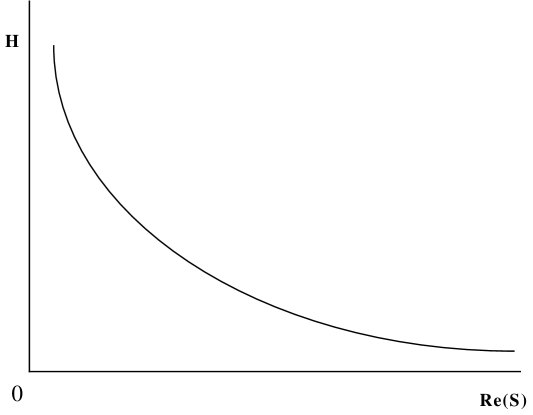
Figure 1: The boundary between the kinematically forbidden (below the curve) and allowed regimes contains the nontrivial minimum of the scalar potential $V(s,h)$.

To see that $\langle W\rangle=0$ at $V=0$, guided by the second numerical result above, we expand $V$ in powers of $m$ in the limit $m\rightarrow 0$. A lengthy but straightforward calculation shows that when $\langle W\rangle=0$, $V\sim{\cal O}(m)+$ higher order as $m\rightarrow 0$; and for $\langle W\rangle\neq 0$, there would be a pole $\sim 1/m$ in $V$ (this is because the threshold corrections at $M_{I}$ cause the Kähler potential to be no longer exactly ‘no-scale’). No such pole was found; the minimum of $V(s,h)$ corresponds to the minimum of $m(s,h)$ (which is zero). The analyical asymptotic expansion of $V$ in $m$, and the numerical results are compatible only for $\langle W\rangle=0$. The reality of the Kähler function, and the hierarchy $M_{cond}\ll M_{I}\ll M_{pl}$ restrict the kinematically allowed region of the parameter space such that:

$$a<\sqrt{2t},\hskip 14.45377pt\lambda a/3\;\gg h$$

(for simplicity, we take both $s$ and $h$ to be real). The kinematically forbidden and allowed regions are typically separated as shown in Fig. 1. The boundary between the two regions contains the nontrivial minimum satisfying $m=0$ and $\langle W\rangle=0$ (as well as the trivial minimum $(s,h)=(\infty,0)$).

Both $m$ and $\langle W\rangle$ increase monotonically from zero in both $h$ and Re$s$ near the vacuum. The plot shown in Fig. 2 shows that $V(s,h)$ also monotonically increases in both directions, and particularly sharply in the $h$ (condensate) direction, indicating confinement. In the direction of the dilaton, the potential increases quadratically as a function of $S$. This can be seen by looking at the $S$-dependence of $V(m\approx 0)$. Furthermore, we notice that the dilaton does ‘run away’, but in the correct direction! Namely, to some finite value of $s$ (which separates the kinematically allowed and forbidden regions, at the nontrivial minimum of the potential). This is in addition to the usual runaway behaviour to $s\rightarrow\infty$, which is the susy-restoring and deconfining limit. Also interesting is the behaviour of $m=2/g_{eff}^{2}(M_{cond})$ near the vacuum, which as noted above, is $m\rightarrow 0$ or $g_{eff}(M_{cond})\rightarrow\infty$ (while $g_{st}$ remains finite). This is exactly what one expects physically, since the condensate — the bound state in the strong coupling regime — is expected to correspond to a stable vacuum solution. Notice, however, that the relations $\langle V\rangle=\langle W\rangle=0$ imply that supersymmetry remains unbroken.

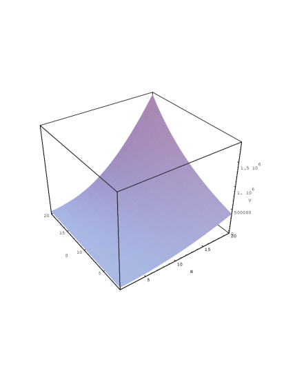
Figure 2: The scalar potential $V(s,h)$. The graph corresponds to the example of $SU(3)$ as the gauge group, and assumimng $\langle t\rangle=1$ for the internal modulus, $\langle a\rangle=1.1$, $\lambda=0.1$, and $\lambda^{\prime}=1$. The kinematically forbidden region of the $h$-$s$ plane has been excluded here; i.e., the minimum of this plot is a point on the curve illustrated in Fig. 1, in this case $({\rm Re}\,s,h)=(2.66,0.00044)$.

So far, the role of the intermediate scale has been masked. In the following, we show that in the effective theory that we are considering, the free parameter $\mu$ in the nonperturbative superpotential (25) is intimately related to the intermediate mass. Furthermore, we shall see that the intermediate mass plays a role in allowing a sensible hierarchy between the Planck scale and condensation scale, consistent with the phenomenologically acceptable values of $\langle$Re$s\rangle$ and $\langle$Re$t\rangle$. For this, we shall give a rough argument below. Of course, the obvious effect that can immediately be associated with the intermediate mass is the shift it causes in the condensation scale, since in its presence the gauge coupling runs differently, as discussed in Section 3.

Figure 3: The runaway behaviour of the dilaton in both directions. In the left direction the minimum corresponds to the effective coupling becoming strong. There, the potentiall ‘runs’ into the kinematically forbidden region.

In the presence $M_{I}$, the vacuum is characterized by two independent conditions:

$$m=0,\hskip 21.68121pt\langle W\rangle=0.$$ (20)

These two conditions together imply that:

$$(t+\bar{t}-|a|^{2})^{\widetilde{\Delta b}/2}\mu^{2b^{<}}\widetilde{M}_{I}^{\Delta b}=1.$$ (21)

Here, $\Delta b=b^{>}-b^{<}$ and $\widetilde{\Delta b}=b-b^{<}$. This can be re-written as follows:

$$s+\bar{s}-bG=b\left[\frac{|\lambda a|}{3}\mu^{b^{<}/\Delta b}\left(t+\bar{t}-|a|^{2}\right)^{\widetilde{\Delta b}/2\Delta b}-1\right]^{-1}.$$ (22)

This equation should be viewed as a relation between $s$, $t$, and $\mu$ in the vacuum of the theory. Is this compatible with phenomenologically acceptable values, $\langle s+\bar{s}\rangle\sim{\cal O}(1)$ and $\langle t+\bar{t}\rangle\sim{\cal O}(1)$? If in eq. (22) we set $\langle t+\bar{t}-|a|^{2}\rangle\simeq 1$, which is also the assumption in the numerical analysis, then it is easy to see that in order to get $\langle s+\bar{s}\rangle\sim{\cal O}(1)$,

$$\frac{\lambda\langle a\rangle}{3}\mu^{-|b^{<}/\Delta b|}-1$$ (23)

should be ${\cal O}(1)$. That is to say, for $b^{<}/\Delta b$ of order unity,

$$\mu\sim\lambda\langle a\rangle\sim{\cal O}(\widetilde{M_{I}}).$$ (24)

The free papramter of the effective superpotential for the condensate is, therefore, ‘locked’ to the intermediate mass. This rough argument also shows that, with some fine tuning, it is at least possible in this scheme to obtain a phenomenologically acceptable value for the dilaton, and at the same time achieve condensation and generate the desired hierarchy. To see this, consider eq. (21) again which together with eq. (24) tells us that:

$$|\langle h\rangle|\sim\exp\left(\frac{-\langle s+\bar{s}\rangle}{6b^{<}}\right)\mu\sim\exp\left(\frac{-\langle s+\bar{s}\rangle}{6b^{<}}\right)\widetilde{M_{I}}.$$ (25)

Again, we see that the parameters, which are admittedly model-dependent but are nevertheless, dictated by the presence of the intermediate mass and the choice of the gauge group can allow for a condensate whose vev is suppressed compared to the parameter $\mu$ which by requirement of phenomenology is of the order of the intermediate mass.

5- Conclusions

Perhaps the most peculiar feature of the model of gaugino condensation that we have discussed above is the running behaviour of the dilaton, which is schematically shown in Fig. 3. The finite value of Re$S$ that the potential “runs” to is, as noted earlier, on the boundary of the kinematically forbidden region, and this value corresponds precisely to $1/g_{eff}(M_{cond})\rightarrow 0$. We interpret this running of Re $S$ in both directions as a manifestation of S-duality which constrains the Kähler potential which we have started with – the behaviour of the strong and weak coupling (small and large $S$, respectively) regimes are alike. The intermediate scale serves basically to shift the renormalization running of the gauge coupling and allow for a hierarchy between the unification and condensation scale by shifting the condensation scale and/or the unification scale (see ref. [4] for detailed discussion of the latter). The intermediate mass (or rather, the vev of the gauge singlet) was assumed, but of course a realistic model should dynamically generate such an $M_{I}$ consistent with phenomenology as discussed near the end of the previous section, and thereby giving a phenomenologically correct hierarchy of scales. This is of course a more significant issue in the models where supersymmetry is broken by gaugino condensation at the scale $M_{cond}$.

However, as we have seen, neither S-duality nor the 1-loop corrections to the dilaton in $K$ (including the dilaton dependent threshold corrections at $M_{I}$ are enough to break supersymmetry in such models. If one is to include any perturbative (1-loop) corrections to $K$, results such as those presented here or in ref. [3] seem to indicate that it is more meaningful to include the full renormalization of the Kähler potential, and all other terms that arise at 1-loop in the supergravity and super-YM effective action which are relevant to gaugino condensation, such as

$$\int d^{4}\theta E(\frac{N_{G}\ln\Lambda^{2}}{32\pi^{2}})(ReS)^{2}|W^{\alpha}W_{\alpha}|^{2}.$$ (26)

These have been recently calculated [19], and work along this direction is under progress elsewhere [20]. Indeed, as it has been argued by Banks and Dine, if stabilization of the dilaton (and other moduli) and supersymmetry breaking are really one and the same phenomena, as they appear to be, then stringy nonperturbative corrections to Kähler potential are crucial and should be included [21]. A realization of this proposal in the context of linear multiplet formulation of gaugino condensate appears in ref [22]. Of course, the exact form of these nonperturbative corrections are not yet understood. But one can perhaps expect that the recent developments in string dualities can shed some light on the latter, and on the stabilization of string moduli and supersymmetry breaking.

Acknowledgements - It is a pleasure to thank Mary K. Gaillard for inspiring this work and all the helpful discussions, and Yi-Yen Wu for collaboration on many parts of this work. This work was supported in part by the Director, Office of Energy Research, Office of High Energy and Nuclear Physics, Division of High Energy Physics of the U.S. Department of Energy under the Contract DE-AC03-76SF00098, and by National Science Foundation under grant PHY-95-14797.

Appendix

S-Duality Transformations

In this appendix, we review some elements of S-duality transformations derived from the general formalism of ref. [2] (see also [3]). In the simplest case, in the presence of a YM field-strength $F_{\mu\nu}$, the scalar fields parameterize the coset space $G/H$, where $G=SL(2,{\cal R})$, is the (noncompact) group of duality transformations and $H$ is its maximal compact subgroup $U(1)$. Under the action of $SL(2,{\cal R})$, the bosonic component of the dilaton transforms in the usual way:

$$s\rightarrow s^{\prime}=\frac{as-ib}{ics+d},$$ (A.1)

where $a,b,c,d$ are real, and $ad-bc=1$. The transformation of the fermions is determined by the considering the invariance of the corresponding kinetic terms and their coupling to the dilaton. One then obtains the trasfomation property of the supermultiplet. As shown in ref. [3], the transformation law (B.1) can be promoted to that of the dilaton (chiral) supermultiplel as follows:

$$S(\theta)\rightarrow\frac{aS(\theta^{\prime})-ib}{icS(\theta^{\prime})+d}=S^{\prime}(\theta^{\prime}),$$ (A.2)

where

$$\theta\rightarrow\theta^{\prime}=\left(\frac{ics+d}{-ic\bar{s}+d}\right)^{1/2}\equiv\xi^{-1/2}\theta,$$ (A.3)

and

$$\psi_{S}\rightarrow\psi_{S}^{\prime}=\xi^{-1/2}(ics+d)^{-2}\psi_{S}.$$ (A.4)

Similarly, for the gaugino one finds:

$$\lambda_{L}\rightarrow\xi^{1/2}(ics+d)\lambda_{L},$$ (A.5)

which implies that:

$$W_{\alpha}(\theta)\rightarrow\xi^{1/2}(ics+d)W_{\alpha}(\theta^{\prime});\hskip 14.45377ptU(\theta)\rightarrow\xi(ics+d)^{2}U(\theta^{\prime}),$$ (A.6)

where $U$ is the composite field containing the gaugino condensate: $U=e^{K/2}H^{3}$. Here, $H$ is the usual chiral multiplet. Note that $U$ and $H$ have different Kähler weights, therefore, $U$ differs from and ordinary chiral superfield; in fact it can be shown to satisfy the constraint $U=(\bar{\cal D}^{2}-8R)V$, where $V$ is a vector multiplet which contains the components of a linear multiplet and a chiral multiplet ([3, 26]).

It follows from the above transformation laws that the chiral field $H$ transforms as:

$$H\rightarrow(ics+d)^{1/3}H.$$ (A.7)

This, together with the fact that Re$S$ $\rightarrow|icS+d|^{-2}$ Re$S$, fixes (up to an S-invariant factor) the function $f(S,\bar{S})$ in the Kähler potential (21): $f=(S+\bar{S})^{1/3}$. Notice that the $T$-moduli are inert under S-duality transformations.

References

- [1] L. Dixon, V. Kaplunovsky, and J. Louis Nucl. Phys. B355: 649 (1991).
- [2] M. K. Gaillard and B. Zumino, Nucl. Phys. B193: 221 (1981); S. Ferrara, J. Scherk., and B. Zumino, Nucl. Phys. 121: 393 (1977).
- [3] P. Binétruy and M.K. Gaillard, Phys. Lett. B365: 87 (1996).
- [4] M. K. Gaillard, and R. Xiu, Phys. Lett. B296: 71 (1992) ; R. Xiu, Phys. Rev. D49: 6656 (1994) ; S. P. Martin and P. Ramond, Phys. Rev. D51: 6515 (1995); K.R. Dienes and A.E. Farraggi, Phys. Rev. Lett. 75: 2646 (1995).
- [5] G. Veneziano and S. Yankielowicz, Phys. Lett. B113: 231 (1982).
- [6] E. Witten, Nucl. Phys. B202: 253 (1982).
- [7] H. P. Nilles, Phys. Lett. B115: 193 (1982); S. Ferrara, L. Girardello, H. P. Nilles, Phys. Lett. B125 457 (1983).
- [8] P. Binétruy and M.K. Gaillard, Phys. Lett. B253: 119 (1991).
- [9] M. Dine, R. Rhom, N. Seiberg, and E. Witten, Phys. Lett. B156: 55 (1985).
- [10] G.L. Cardoso and B.A. Ovrut, Nucl. Phys. B369: 351 (1992); ibid., Nucl. Phys. B392: 315 (1993); ibid.,Nucl. Phys. B418: 535 (1994); S. Ferrara abd M. Villasante, Phys. Lett. B186: 87 (1987); P. Binétruy, G. Girardi, R. Grimm and M. Müller, Phys. Lett. B265 111 (1991); P. Adamietz, P. Binétruy, G. Girardi and R. Grimm, Nucl. Phys. B401: 257 (1993); J.P. Derendinger, F. Quevedo, M. Quirós, Nucl. Phys. B428: 228 (1994).
- [11] I. Antoniadis, K.S. Narain, and T.R. Taylor, Phys. Lett. B267: 37 (1991).
- [12] M.K. Gaillard and T.R. Taylor, Nucl. Phys. B381: 577 (1992).
- [13] A. Font, L. I. Ibáñez, D. Lüst, F. Quevedo, Phys. Lett. 241: 35 (1990).
- [14] A. Sen, Int. J. Mod. Phys. A9: 3707 (1994), J. H. Schwarz and A. Sen, Phys. Lett. B312: 105 (1993); Phys. Lett. B411: 105 (1994); I. Girardello, A. Giveon, M. Porratti, A. Zaffaroni, Nucl. Phys. B448 127 (1995).
- [15] Z. Lalak, A. Niemeyer, H. P. Nilles, Nucl. Phys.B453: 100, 1995.
- [16] B. de Carlos, J. Casas, and C. Muñoz, Phys. Lett. B263: 248 (1991); D. Lüst and C. Muñoz, CERN-Th 6358/91 (1991).
- [17] S. Chaudhuri, G. Hockney, and J. Lykken, Nucl. Phys.B469: 357 (1996).
- [18] V. Kaplunovsky and J. Louis, Nucl. Phys. B422: 57 (1994).
- [19] M.K. Gaillard, V. Jain, and K. Saririan, preprint LBL-34984, hep-th/9606052 (to be published in Phys. Rev. D); Also, Phys. Lett.B387: 520 (1996).
- [20] K. Saririan, in Progress.
- [21] T. Banks and M. Dine, Phys. Rev. D:50 7454 (1994).
- [22] P. Binétruy, M. K. Gaillard and Y-Y. Wu, preprint LBNL-38590, UCB-PTH 96/13; hep-th/9605170 (to be published in Nucl. Phys. B).
- [23] P. Binétruy, G. Girardi, R. Grimm and M. Müller, Phys. Lett. 189B: 83 (1987); P. Binétruy, G. Girardi and R. Grimm, Annecy preprint LAPP-TH-275-90, (1990).
- [24] M. A. Shifman and A. I. Vainshtein, Nucl. Phys. B277: 456 (1986); and Nucl. Phys. B359: 571 (1991).
- [25] V. Kaplunovsky and J. Louis, Nucl. Phys. B444: 191 (1995).
- [26] P. Binétruy, M. K. Gaillard, and T. Taylor, Nucl. Phys. B455: 97 (1995).