Quantum effects on winding configurations
in $SU(2)$-Higgs theory

Abstract

We examine the quantum corrections to the static energy for Higgs winding configurations in order to ascertain whether such corrections may stabilize solitons in the standard model. We evaluate the effective action for winding configurations in Weinberg-Salam theory without $U(1)$-gauge fields or fermions. For a configuration whose size, $a\ll m^{-1}$ where $m=\max\{m_{W},m_{H}\}$, $m_{W}$ is the W-mass, and $m_{H}$ is the Higgs mass, the static energy goes like $g^{-2}m_{W}^{2}a[1+b_{0}g^{2}\ln(1/ma)]^{c_{0}/b_{0}}$ in the semiclassical limit. Here $g$ is the $SU(2)$-gauge coupling constant and $b_{0},c_{0}$ are positive numbers determined by renormalization-group techniques. We discuss the limitations of this result for extremely small configurations and conclude that quantum fluctuations do not stabilize winding configurations where we have confidence in $SU(2)$-Higgs as a renormalizable field theory.

CTP#2585 Submitted to Physical Review D

hep-th/9611059 Typeset in REVTeX

I Introduction

The Higgs sector in the standard model is a linear sigma model. Such a theory exhibits configurations of nontrivial winding, though they are not stable. In the standard model, winding configurations shrink to some small size and then unwind via a Higgs zero when allowed to evolve by the Euler-Lagrange equations. These winding configurations can be stabilized if one introduces four-derivative Higgs self-interaction terms which are not present in the standard model [1, 2]. The motivation typically cited for introducing such terms is that one may treat the Higgs sector of the Lagrangian as an effective field theory of some more fundamental theory which only manifests itself explicitly at some high energy scale. The stabilized configurations have phenomenological consequences in electroweak processes and provide an arena for testing nonperturbative aspects of field theory and the standard model. The presence of gauge fields leads to the instability of these solitons [2], and their decay, whether induced or by quantum tunnelling, is associated with fermion number violation [2, 3]. In turn, such a mechanism for fermion number violation may have an effect on the early universe and electroweak baryogenesis [4].

Unfortunately, the procedure just described for stabilization is inconsistent. First, treating the Higgs sector as an effective theory requires the inclusion of all higher-derivative terms of a given dimension rather than just a few. Moreover, using an effective field theory to stabilize solitons creates difficulties. Effective field theories are equivalent to derivative expansions. Solitons that are stabilized by introducing the leading-order terms in a derivative expansion imply that the following orders in the expansion will contribute equally as the leading orders. Truncating the derivative expansion, then, is not legitimate.

We will take a different approach; we wish to see whether just the quantum fluctuations of a renormalizable $SU(2)$-Higgs theory can stabilize winding configurations. We will take the Higgs sector to be that found in the standard model. Consider just the mode associated with the size of a given winding configuration. That mode may be parametrized by the quantity $a$, the spatial size of the object (which must be positive). The potential for that degree of freedom goes like $a+a^{3}$ and energetically favors configurations of zero size. Classically, the degree of freedom will evolve towards $a=0$ while losing its energy to radiative modes. Now let us quantize this mode. Even though the system would favor being at $a=0$, that would also imply the momentum conjugate to that degree of freedom would also be zero. Heisenberg uncertainty would puff out the expectation value of the size degree of freedom. Note that the size of the soliton will be proportional to Planck’s constant to some power. The mechanism described is analagous to that which stabilizes the atom, which is classically unstable. Of course, there are other modes that couple into our situation, making the analysis more complex. Work has been done [5] that investigates quantizing breathing modes in sigma models such as the Higgs sector of the standard model.

In this paper, we identify the quantum effects on the energy of static winding configurations by evaluating the effective action. If quantum effects stabilize solitons, that effect should be reflected by some extremum in the effective action. If we take the weak gauge-coupling limit, $g^{2}\rightarrow 0$, we shall see that an analytic expression is available for the effective action that is a controlled approximation in the regime where we have confidence in $SU(2)$-Higgs theory as a renormalizable field theory. The weak coupling limit is equivalent to the semiclassical limit when fields are scaled properly. When Planck’s constant is small, we need only focus on small field configurations. This observation follows from the scenario described above for stabilizing winding configurations by quantum fluctuations: the size of a stabilized object will be proportional to Planck’s constant, and therefore, will be small if it exists.

Evaluating corrections to energies via the effective action is not a new approach. It has been a focus of investigation in effective meson theories [6, 7] and other areas [8]. Although, they elucidate important effects, such as bosonic and fermionic back-reaction as well as valence fermion effects, these studies treat the effective action to one-loop order only. We will see that there is a difficulty with simultaneously examining small configurations and neglecting higher-loop effects.

We begin by spelling out the action and types of configurations under consideration. When configuration sizes are small, we can employ renormalization-group techniques to ascertain the asymptotic behavior of the one-particle irreducible green’s functions which, in turn, allows us to determine the leading-order size dependence of the effective action. We will find our results to be reliable until the size of our configuration becomes extremely small, on the order of the inverse momentum of the Landau pole associated with the Higgs sector. Thus our results are valid when the size of our configuration is not on the order of the cutoff necessary to avoid a trivial renormalized Higgs self-coupling. We conclude that the quantum corrections to the energy are not sufficient to stabilize Higgs winding configurations where we have confidence in $SU(2)$-Higgs as a renormalizable field theory.

II The Effective Action

Consider the Weinberg-Salam theory of electroweak interactions, neglecting the $U(1)$-gauge fields and fermions. Our field variables form the set $\{A_{\mu}(x),\phi(x)\}$ where the gauge field $A_{\mu}(x)=\sigma^{a}A_{\mu a}(x)/2$ is in the adjoint representation of $SU(2)$ ($\{\sigma^{a}\}$ are the Pauli matrices), and the Higgs field $\phi(x)$ is in the fundamental representation of $SU(2)$. The classical action we consider is

$$S = S_{0}+S_{gf}$$ (1)

$$S_{0} = \int d^{4}x\left\{-\frac{1}{4}F^{\mu\nu}_{a}F^{a}_{\mu\nu}+\left({\cal D}^{\mu}\phi\right)^{\dagger}\left({\cal D}_{\mu}\phi\right)-\frac{g^{2}\alpha}{2}\left[(\phi+\phi_{0})^{\dagger}(\phi+\phi_{0})-\frac{m_{W}^{2}}{g^{2}}\right]^{2}\right\}$$ (2)

$$S_{gf} = -\frac{1}{2\xi}\int d^{4}x\left[\partial_{\mu}A^{\mu a}+ig^{2}\xi\left(\phi^{\dagger}\sigma^{a}\phi_{0}-\phi^{\dagger}_{0}\sigma^{a}\phi\right)\right]^{2}$$ (3)

where we have chosen the $R_{\xi}$-gauge and

$${\cal D}_{\mu}\phi = (\partial_{\mu}-\frac{ig}{2}\sigma^{a}A_{\mu a})\phi,$$ (4)

$$F^{a}_{\mu\nu} = \partial_{\mu}A^{a}_{\nu}-\partial_{\nu}A^{a}_{\mu}+g\epsilon^{abc}A_{\mu b}A_{\nu c}.$$ (5)

We have shifted $\phi(x)$ by a vacuum configuration $\phi_{0}$, some constant $SU(2)$-doublet satisfying the relationship $\phi_{0}^{\dagger}\phi_{0}=m_{W}^{2}/g^{2}$. The parameter $m_{W}$ is the mass of the gauge field and $\alpha=(m_{H}/m_{W})^{2}$ where $m_{H}$ is the physical Higgs mass. The Feyman rules derived from (2) are familiar. In this analysis, we restrict ourselves to the semiclassical limit, which is equivalent to taking $g^{2}\rightarrow 0$ while holding $m_{W},m_{H}$ (and, thus, also $\alpha$) fixed.

We wish to determine the effects of quantum fluctuations on Higgs winding configurations. We will evaluate the effective action, $\Gamma[A^{a}_{\mu},\phi]$, where

$$A^{a}_{\mu}(x) = 0$$ (6)

$$\phi(x) = \left[U({\bf x})-1\right]\phi_{0}$$ (7)

and where $U({\bf x})\in SU(2)$ is a static configuration such that $U({\bf x})\rightarrow 1$ as $|{\bf x}|\rightarrow\infty$ with characteristic size, $a$. We require the field $U({\bf x})$ to be a configuration of unit winding number

$$w[U]=\frac{1}{24\pi^{2}}\int d^{3}{\bf x}\ \epsilon^{ijk}{\rm Tr}\left[(U^{\dagger}\partial_{i}U)(U^{\dagger}\partial_{j}U)(U^{\dagger}\partial_{k}U)\right]=1.$$

From conventional perturbation theory, we know that

$$\Gamma[\phi]=\sum_{n}\int\frac{d^{4}p_{1}}{(2\pi)^{4}}\cdots\frac{d^{4}p_{n}}{(2\pi)^{4}}(2\pi)^{4}\delta^{4}\left(\sum_{i}p_{i}\right)\Gamma^{(n)}(\{p_{i}\})\hat{\phi}(p_{1})\cdots\hat{\phi}(p_{n})$$ (8)

where $\Gamma^{(n)}(\{p_{i}\})$ are the one-particle irreducible green’s functions with $n$ external $\phi$’s. We define the field $\hat{\phi}(p)$ as the fourier transform of $\phi(x)$. For the configuration (7), we get

$$\hat{\phi}(p)=2\pi\delta(p_{0})\int d^{3}{\bf x}\ e^{-i{\bf p}\cdot{\bf x}}\phi({\bf x}).$$

The static energy for the state whose expectation value of the operator associated with the Higgs field is $\phi({\bf x})$ will be the quantity $E$ in the expression

$$\Gamma[\phi]=-\int dt\ E.$$

Normally, the effective action (8) cannot be evaluated exactly. However, because we are investigating the semiclassical limit, we are only interested in a configuration whose size, $a$, is small. We find that under such a circumstance, we may use the Callan-Symanzik equation for our theory to evaluate the leading-order size dependence of the one-particle irreducible green’s functions in (8) and thus evaluate the quantum corrections to the static energy.

III Asymptotic Behavior

In this section we identify the scaling dependence of the one-particle irreducible green’s functions, $\Gamma^{(n)}(\{p_{i}\})$, when the characteristic size of the Higgs winding configuration, $a$, is small with respect to both mass scales of the theory. Let $m=\max\{m_{W},m_{H}\}$. We implement the condition of small, static background configurations by requiring the field $\hat{\phi}(p)$ to have support only for $p_{0}=0$ and $|{\bf p}|\gg m$ which implies $0<m^{2}\ll-p^{2}$. Under this circumstance, the asymptotic dependence of $\Gamma^{(n)}$ will be determined by the Callan-Symanzik equation [9]

$$\left[\frac{\partial}{\partial s}-\beta_{g}(g^{2},\alpha)\frac{\partial}{\partial g^{2}}-\beta_{\alpha}(g^{2},\alpha)\frac{\partial}{\partial\alpha}+n\gamma(g^{2},\alpha)+(n-4)\right]\Gamma^{(n)}(\{e^{s}\tilde{p}_{i}\},g^{2},\alpha,m)=0.$$ (9)

where $s=\ln(1/ma)$ and $-{\tilde{p}_{i}}^{2}\sim m^{2}$. Here $\beta_{g},\beta_{\alpha}$ are the beta functions for $g^{2}$ and $\alpha$, respectively, that determine the running couplings. The function $\gamma(g^{2},\alpha)$ is the anomalous dimension of the scalar field $\phi(x)$.

The solution to (9) may be determined by the method of characteristics. We find that

$$\Gamma^{(n)}_{asymp}=(ma)^{n-4}\Gamma^{(n)}(\{\tilde{p}_{i}\},\bar{g}^{2}(s,g^{2},\alpha),\bar{\alpha}(s,g^{2},\alpha),m)\ \ \ \ \ \ \ \ \ \ \ \ \ \ \$$ (10)

$$\ \ \ \ \ \ \ \ \ \ \times\exp\left[-n\int_{0}^{s}d\sigma\ \gamma(\sigma,\bar{g}^{2}(\sigma,g^{2},\alpha),\bar{\alpha}(\sigma,g^{2},\alpha))\right]$$ (11)

where the running coupling constants $\bar{g}^{2},\bar{\alpha}$ are defined such that

$$\frac{d\bar{g}^{2}}{ds}=\beta_{g}(\bar{g}^{2},\bar{\alpha}),\ \ \ \ \ \ \frac{d\bar{\alpha}}{ds}=\beta_{\alpha}(\bar{g}^{2},\bar{\alpha})$$

and $\bar{g}^{2}(s=0)=g^{2},\bar{\alpha}(s=0)=\alpha$. We will evaluate (11) using one-loop beta functions and scalar anomalous dimension.

The one-loop beta functions may be easily obtained from the literature. For a single scalar Higgs doublet, we find [10]

$$\beta_{g}(g^{2},\alpha) = -b_{0}g^{4}$$ (12)

$$\beta_{\alpha}(g^{2},\alpha) = g^{2}(A\alpha^{2}+B\alpha+C)$$ (13)

where $b_{0}=43/48\pi^{2},A=3/4\pi^{2},B=1/3\pi^{2},C=9/64\pi^{2}$.

FIG. 1.: One-loop contribution to the scalar field anomalous dimension.

The one-loop anomalous dimension may be evaluated using just the graph in Figure 1.

$$\gamma(g^{2},\alpha)=-\frac{1}{2}c_{0}g^{2}$$ (14)

where $c_{0}=3[1+(\xi-1)/4]/16\pi^{2}$. Because $\xi$ is positive or zero, $c_{0}\geq 9/64\pi^{2}$. Inserting these expressions into (11), we find that

$$\Gamma^{(n)}_{asymp}=(ma)^{n-4}\Gamma^{(n)}(\{\tilde{p}_{i}\},\bar{g}^{2},\bar{\alpha})\left(1+b_{0}g^{2}s\right)^{\frac{nc_{0}}{2b_{0}}}.$$

When $n>4$, the one-loop $n$-point diagrams give the leading terms for the prefactor

$$\Gamma^{(n)}(\{\tilde{p}_{i}\},g^{2},\alpha)\sim m^{4-n}g^{n}F_{n}(\sqrt{\alpha})$$ (15)

where $F_{n}$ is a polynomial in $\sqrt{\alpha}$ of order $n$. When $n\leq 4$, the renormalized $\Gamma^{(n)}$ is dominated by the classical contribution

$$\Gamma^{(2)}(\tilde{p},g^{2},\alpha)\sim m^{2},\ \ \ \Gamma^{(3)}(\{\tilde{p}_{i}\},g^{2},\alpha)\sim m_{W}g\alpha,\ \ \ \Gamma^{(4)}(\{\tilde{p}_{i}\},g^{2},\alpha)\sim g^{2}\alpha.$$ (16)

We are now prepared to insert these asymptotic formulas into (8). So long as $\bar{\alpha}/\alpha$ is not too large, the leading-order size dependence of the effective action comes from the two-point one-particle irreducible greens function. All other terms are supressed by powers of $a$ and other factors. The leading-order contribution to the effective action from quantum fluctuations yields

$$\Gamma[\phi]=\int\frac{d^{4}p}{(2\pi)^{4}}\phi^{\dagger}(p)\phi(p)p^{2}\left[1+\frac{1}{2}b_{0}g^{2}\ln\left(\frac{-p^{2}}{m^{2}}\right)\right]^{\frac{c_{0}}{b_{0}}}$$ (17)

implying a scale dependence

$$\Gamma[\phi]\sim-\int dt\ \frac{m_{W}^{2}a}{g^{2}}\left[1+b_{0}g^{2}\ln\left(\frac{1}{ma}\right)\right]^{\frac{c_{0}}{b_{0}}}.$$ (18)

One can recover the classical result from (18) by setting the $g^{2}$ inside the brackets to zero. Note that when $b_{0}g^{2}\ln(\frac{1}{ma})\sim 1$, the quantum corrections to the energy are as significant as the classical contribution. Nevertheless, the static energy that corresponds to this effective action is a monotonically increasing function of the size, $a$, such that $E(a=0)=0$. This would imply that Higgs winding configurations would shrink to zero size and unwind via a Higgs zero, just as in the classical scenario.

Let us take a closer look at our expression for the leading contribution to the effective action (17). Expanding in powers of $g^{2}$ we get

$$\Gamma[\phi]=\int\frac{d^{4}p}{(2\pi)^{4}}\phi^{\dagger}(p)\phi(p)p^{2}+\frac{c_{0}}{2}g^{2}\int\frac{d^{4}p}{(2\pi)^{4}}\phi^{\dagger}(p)\phi(p)p^{2}\ln\left(\frac{-p^{2}}{m^{2}}\right)+\cdots$$

The first term is the contribution from the classical action. The next term is the leading order contribution from one-loop one-particle irreducible graphs. Note that it depends only on $c_{0}$. In fact, the dominant one-loop contribution to the effective action comes from the graph in Figure 1. The scale dependence of the static energy will go like

$$E=\frac{m_{W}^{2}a}{g^{2}}\left[{\cal A}+{\cal B}g^{2}\ln\frac{1}{ma}+{\cal C}g^{4}\left(\ln\frac{1}{ma}\right)^{2}+\cdots\right]$$ (19)

where $\cal A,\cal B,\cal C$ are numbers. Again the first term is the classical energy, the second is the one-loop energy, and the rest of the terms in the expansion (19) correspond to higher-loop energies order by order. We can see by comparing (18) with (19) that loop contributions to the effective action beyond one loop can only be neglected when $b_{0}g^{2}\ln(1/ma)\ll 1$. However, that is precisely the condition where the one-loop contribution can be neglected relative to the classical action. Thus, drawing conclusions concerning solitons based on one-loop results may be difficult. When dealing with small configurations, one still needs to include higher-loop contributions, even in the semiclassical limit.

IV Limitations

We expect the expression (18) to be valid so long as we can neglect high-loop contributions to the beta functions (12–13), the anomalous dimension (14), and the renormalized greens functions (15–16). Higher loop contributions to these quantitities will be negligible if the running couplings associated with the gauge coupling, $\bar{g}^{2}$, and that associated with the scalar self-coupling, $\bar{g}^{2}\bar{\alpha}$, are small. The first criterion is relatively easy to adhere to, since the gauge coupling is asymptotically free and will run to zero with increasingly small sized configurations, subject to $\bar{g}^{2}\bar{\alpha}$ being small. Recall also, we require that $\bar{\alpha}/\alpha$ not be too large so that we may neglect all but the two-point contribution to the effective action. All these criteria for the validity of (18) hinge on how $\bar{\alpha}$ runs with smaller and smaller sized configurations. From (13) we can ascertain the dependence of $\bar{\alpha}$ on the configuration size. Inserting the appropriate expression for $\bar{g}^{2}$, we find

$$\bar{\alpha}(s,g^{2},\alpha)=\frac{1}{2A}\left\{-B+D\tan\left[\tan^{-1}\frac{2A\alpha+B}{D}+\frac{D}{2b_{0}}\ln(1+b_{0}g^{2}s)\right]\right\}$$ (20)

where $D=\sqrt{4AC-B^{2}}>0$. Thus we see that $\bar{\alpha}$ has a Landau singularity when the argument of the tangent is $\pi/2$. Thus, the expression (18) is certain to break down for a configuration of some size approaching the inverse momentum associated with this singularity. However, if the argument of the tangent is not very close to $\pi/2$, then $\bar{\alpha}$ will not be numerically very different from the renormalized $\alpha$, implying that $\bar{g}^{2}\bar{\alpha}$ is small if $g^{2}\alpha$ is small. Thus, our constraint on the size, $a$, will be that

$$\tan^{-1}\frac{2A\alpha+B}{D}+\frac{D}{2b_{0}}\ln(1+b_{0}g^{2}s)<\frac{\pi}{2}.$$

This implies that

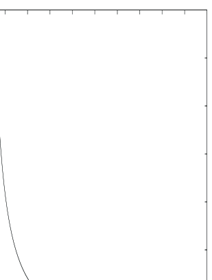
FIG. 2.: The function $f(\alpha)$ is plotted versus $\alpha={m_{H}}^{2}/m^{2}$. The scale of the Landau pole may be extracted from this curve using the identity $f(\alpha)=b_{0}g^{2}\ln(\Lambda_{Landau}/m)$. The criterion for the validity of our expression for the quantum-corrected energy is that $a>1/\Lambda_{Landau}$ or, alternatively, $a>m^{-1}\exp[-f(\alpha)/b_{0}g^{2}]$.

$$b_{0}g^{2}s<e^{\frac{2b_{0}}{D}\left[\frac{\pi}{2}-\tan^{-1}\frac{2A\alpha+B}{D}\right]}-1\equiv f(\alpha).$$

The function, $f(\alpha)$ is plotted in Figure 2. Thus, our expression (18) is valid for configurations whose size, $a$, satisfies

$$m^{-1}\ e^{-f(\alpha)/b_{0}g^{2}}\ll a\ll m^{-1}$$ (21)

when $g^{2},g^{2}\alpha\ll 1$. Recall from our discussion at the end of the last section that the quantum corrections to the energy will be as significant as the classical contribution when $b_{0}g^{2}s\sim 1$. Now we can see from our condition $b_{0}g^{2}s<f(\alpha)$ and Figure 2 that there exists some $\alpha_{max}$ such that if $\alpha<\alpha_{max}$, the energy (18) will be both reliable and significantly different than the classical result. When $\alpha>\alpha_{max}$ the quantum corrections are bound to be small where our result is valid.

When the size of the configuration is near the inverse momentum associated with the Landau pole, higher-loop contributions to the beta and gamma functions become important and potentially change the size-dependence of the energy. However, if we take the presence of this singularity as a cue that a finite momentum cutoff is necessary to maintain a nontrivial Higgs self-coupling [12], then we can conclude that our expression for the static energy (18) is valid so long as the size of the configuration is not so small as to be on the order of a lattice size associated with a finite momentum cutoff. Thus, quantum fluctuations do not stabilize winding configurations where we have confidence in $SU(2)$-Higgs theory as a renormalizable field theory.

V Concluding Remarks

We evaluate the quantum corrections to the static energy for a Higgs winding configuration in the semiclassical limit. We ascertain the leading-order contributions to the static energy which is relevant to soliton stabilization by treating the effective action for small-sized configurations. Moreover, we perform this calculation in such a way that avoids the difficulties in neglecting higher-loop contributions to the effective action. By solving the Callan-Symanzik equation for our theory, we find the leading-order size dependence of the energy including quantum corrections. We also use renormalization-group techniques to determine the limitations on our expression.

We find that bosonic quantum fluctuations do not stabilize Higgs winding configurations in a standard model type $SU(2)$-Higgs theory. Classically, a configuration of size, $a$, would have static energy which goes like $m_{W}^{2}a/g^{2}$. These winding configurations will shrink to zero size and eventually unwind via a Higgs zero. Including quantum fluctuations, when $a\ll m\equiv\max\{m_{W},m_{H}\}$, the corrected energy goes like $g^{-2}m_{W}^{2}a[1+b_{0}g^{2}\ln(1/ma)]^{c_{0}/b_{0}}$, where $b_{0},c_{0}$ are positive numbers. The corrected energy still goes to zero as the size, $a$, goes to zero. When the configuration shrinks to a size, $a\sim m^{-1}\exp[-f({m_{H}}^{2}/m_{W}^{2})/b_{0}g^{2}]$, our result becomes invalid and we run into the Landau pole associated with the Higgs sector. Taking this pole to be an indication that a finite momentum cutoff is necessary for a nontrivial Higgs self-coupling, we find that bosonic quantum fluctuations do not stabilize Higgs winding configurations where we have confidence in $SU(2)$-Higgs theory as a renormalizable field theory.