TASI LECTURES ON D-BRANES

Abstract

This is an introduction to the properties of D-branes, topological defects in string theory on which string endpoints can live. D-branes provide a simple description of various nonperturbative objects required by string duality, and give new insight into the quantum mechanics of black holes and the nature of spacetime at the shortest distances. The first two thirds of these lectures closely follow the earlier ITP lectures hep-th/9602052, written with S. Chaudhuri and C. Johnson. The final third includes more extensive applications to string duality.

D-branes are extended objects, topological defects in a sense, defined by the property that strings can end on them. One way to see that these objects must be present in string theory is by studying the $R\to 0$ limit of open string theory, where the different behaviors of open and closed strings lead to a seeming paradox.[1] From the study of this limit one can argue that the usual Type I, Type IIA and Type IIB string theories are different states in a single theory, which also contains states with arbitrary configurations of D-branes. Moreover this argument is purely perturbative, in that it does not require any strong-coupling continuation or use of the BPS property.

However, this subject remained obscure until the advent of string duality. It was then observed that D-branes have precisely the correct properties to fill out duality multiplets,[2] whose other members are fundamental string states and ordinary field-theoretic solitons. Further, they are much simpler than ordinary solitons, and their bound states and other properties can be understood more explicitly. Even before the role of D-branes was realized, the circumstantial evidence for string duality was extremely strong. D-branes have extended this by providing a much more complete and detailed dynamical picture. Beyond the simple verification of weak/strong duality, D-branes have given surprising and still developing insight into the quantum mechanics of black holes and into the nature of spacetime at the shortest distance scales.

The first three lectures develop the basic properties of D-branes. The approach follows ref. 1, coming upon D-branes by way of $T$-duality. Lecture 1 is a review of open and unoriented bosonic strings, lecture 2 develops the effect of $T$-duality in these theories, and lecture 3 extends these results to the superstring. The final two lectures develop various more advanced ideas as well as applications to string duality.

These lectures are an expanded and updated version of an earlier set of notes from lectures given at the ITP, which were written up with Shyamoli Chaudhuri and Clifford Johnson.[3] The first two thirds of the present lectures closely follow those notes. The final third gives a more detailed treatment of the application to string duality. New or extended subjects include D-brane actions, D-brane bound states, the connection to M theory and U-duality, and D-branes as instantons, as probes, and as black holes. Obviously, given constraints of space and time, the discussion of each of these subjects is somewhat abbreviated.

1 Lecture 1: Open and Unoriented Bosonic Strings

The weakly coupled $E_{8}\times E_{8}$ heterotic string on a Calabi-Yau manifold is strikingly similar to the grand unified Standard Model. Thus, the focus after the 1984 revolution was on this closed oriented string theory. We must therefore begin with an introduction to the special features of open and unoriented strings.

1.1 Open Strings

To parameterize the open string world sheet, let the ‘spatial’ coordinate run $0\leq\sigma^{1}\leq\pi$. In conformal gauge, the action is

$${1\over 4\pi\alpha^{\prime}}\int_{\cal M}d^{2}\sigma\,\partial_{a}X^{\mu}\partial_{a}X_{\mu}.$$ (1)

Varying $X^{\mu}$ and integrating by parts,

$$\delta S=-{1\over 2\pi\alpha^{\prime}}\int_{\cal M}d^{2}\sigma\,\delta X^{\mu}\partial^{2}X_{\mu}\ +\ {1\over 2\pi\alpha^{\prime}}\int_{\partial M}d\sigma\,\delta X^{\mu}\partial_{n}X_{\mu}$$ (2)

where $\partial_{n}$ is the derivative normal to the boundary. The bulk term in the variation (2) gives Laplace’s equation (or the wave equation, if we have Minkowski signature on the world-sheet.) At the boundary, the only Poincaré invariant condition is the Neumann condition

$$\partial_{n}X^{\mu}=0.$$ (3)

The Dirichlet condition $X^{\mu}={\rm constant}$ is also consistent with the equation of motion and we might study it directly. However, we have chosen to follow the approach of ref. 1, beginning with the Neumann condition and finding that the Dirichlet condition is forced on us by $T$-duality. This is a good pedagogic route, as the various properties of D-branes make their appearance in a natural way. It also shows that D-branes are necessarily part of the spectrum of string theory, as one can start from the ordinary open string vacuum and by a continuous change of parameters ($R\to 0$) get to a state containing D-branes.

We should mention some early papers [4] in which Dirichlet conditions were investigated as a potentially interesting variation of string theory in their own right. The association of the Dirichlet condition with an actual hyperplane in spacetime came later, in the context of compactification of open string theory.[5]${}^{\!,\,}$[6] It was then observed that the hyperplane was a dynamical object [1], hence ‘D-brane,’ and that it could be produced via T-duality.[1]${}^{\!,\,}$[7]${}^{\!,\,}$[8]

The papers in the previous paragraph kept the Neumann condition for the time coordinate (and usually for some spatial coordinates) so that they defined an object, the D-brane. Fully Dirichlet conditions define the D-instanton. These boundary conditions were originally interpreted in terms of an off-shell probe of string theory.[9] It was then proposed to modify string theory by the inclusion of a gas of such objects, changing the short distance structure.[10] It was later argued [11] that such D-instantons were a necessary part of string theory and carried the combinatoric weight $e^{-O(1/g)}$ associated with large stringy nonperturbative effects.[12] It was also observed that the D-instanton breaks half the supersymmetries.[13]

The general solution to Laplace’s equation with Neumann boundary conditions is

$$X^{\mu}(z,{\bar{z}})=x^{\mu}-i\alpha^{\prime}p^{\mu}\ln(z{\bar{z}})+i\sqrt{\alpha^{\prime}\over 2}\sum_{m\neq 0}{\alpha_{m}^{\mu}\over m}(z^{-m}+{\bar{z}}^{-m}),$$ (4)

where $x^{\mu}$ and $p^{\mu}$ are the position and momentum of the center of mass. As is conventional in conformal field theory, this has been written in terms of the coordinate $z=e^{\sigma^{2}-i\sigma^{1}}$, so that time runs radially. The usual canonical quantization gives the commutators

$$[x^{\mu},p^{\nu}] = i\eta^{\mu\nu},$$

$${}[\alpha_{m}^{\mu},\alpha_{n}^{\nu}] = m\delta_{m+n}\eta^{\mu\nu}.$$ (5)

The mass shell condition is

$$M^{2}=-p^{\mu}p_{\mu}={1\over\alpha^{\prime}}\left(\sum_{m=1}^{\infty}mN_{m}-1\right).$$ (6)

Here $N_{m}$ is the number of excited oscillators in the $m^{th}$ mode, and the $-1$ is the zero point energy of the physical bosons. Let us remind the reader of the mnemonic for zero point energies. A boson with periodic boundary conditions has zero point energy $-{1\over 24}$, and with antiperiodic boundary conditions it is $1\over 48$. For fermions, there is an extra minus sign. For the bosonic string in 26 dimensions, there are 24 transverse (physical) degrees of freedom, for a total of $-{24\over 24}=-1$.

For example, the two lightest particle states and their vertex operators are

$${\rm tachyon} |{k}\rangle,\quad M^{2}=-{1/\alpha^{\prime}},\quad V=\exp({i{k}\cdot{X}})$$

$${\rm photon} \alpha^{\mu}_{-1}|{k}\rangle,\quad M^{2}=0,\quad V^{\mu}=\partial_{t}X^{\mu}\exp({i{k}\cdot{X}}).$$ (7)

Here $\partial_{t}$ is the derivative tangent to the string’s world sheet boundary. The open string vertex operators are integrated only over the world-sheet boundary as is evident in figure 1b.

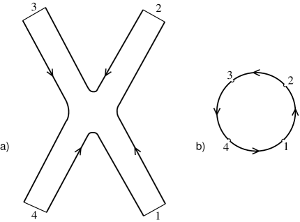
Figure 1: a) Scattering of open strings. b) Conformally transformed world-sheet.

1.2 Chan-Paton Factors

It is consistent with spacetime Poincaré invariance and world-sheet conformal invariance to add non-dynamical degrees of freedom to the ends of the string. Their Hamiltonian vanishes so these Chan-Paton degrees of freedom have no dynamics—an end of the string prepared in one of these states will remain in that state. So in addition to the usual Fock space label for the state of the string, each end is in a state $i$ or $j$ where the labels run from $1$ to $N$.

Figure 2: Open string with Chan-Paton degrees of freedom.

The $n\times n$ matrices $\lambda^{a}_{ij}$ form a basis into which to decompose a string wavefunction

$$|{k};a\rangle=\sum^{N}_{i,j=1}|{k},ij\rangle\lambda^{a}_{ij}.$$ (8)

These wavefunctions are the Chan-Paton factors.[14] Each vertex operator carries such a factor. The tree diagram for four oriented strings s shown in figure 1. Since the Chan-Paton degrees of freedom are non-dynamical, the right end of string 1 must be in the same state as the left end of string 2, and so on. Summing over all basis states then gives a trace of the product of Chan-Paton factors,

$$\lambda^{1}_{ij}\lambda^{2}_{jk}\lambda^{3}_{kl}\lambda^{4}_{li}={\rm Tr}(\lambda^{1}\lambda^{2}\lambda^{3}\lambda^{4}).$$ (9)

Such a trace appears in each open string amplitude. All such amplitudes are invariant under a the $U(N)$ symmetry 

$$\lambda^{i}\ \to\ U\lambda^{i}U^{-1},$$ (10)

under which the endpoints transform as $N$ and $\bar{\mbox{\boldmath$N$}}$. The massless vector vertex operator $V^{a\mu}=\lambda^{a}_{ij}\partial_{t}X^{\mu}\exp(i{k}\cdot{X})$ transforms as the adjoint under the $U(N)$ symmetry, so (as is generally the case in string theory) this global symmetry of the world-sheet theory is elevated to a gauge symmetry in spacetime.

The massless bosonic fields are the graviton $G_{\mu\nu}$, dilaton $\phi$, antisymmetric tensor $B_{\mu\nu}$, and vector $A^{\mu}$. The closed string coupling is related to the expectation value of the dilaton field $\phi_{0}$ by $g=e^{\phi_{0}}$. In the low energy limit, the massless fields satisfy equations of motion that may be obtained by varying the action

$$S = \int d^{10}x\left\{{1\over 2\kappa_{0}^{2}}e^{-2\phi}\left(R+4(\nabla\phi)^{2}-{1\over 12}H_{\mu\nu\kappa}H^{\mu\nu\kappa}\right)\right.$$ (11)

$$\qquad\qquad\qquad\qquad-{c\over 4}e^{-\phi}{\rm Tr}F_{\mu\nu}F^{\mu\nu}+O(\alpha^{\prime})\biggl{\}}\ .$$

This action arises at tree level in string perturbation theory. The dimensionful constant $\kappa_{0}$ is arbitrary, though in the context of string duality there will be a natural additive normalization for $\phi$ and so a natural value for $\kappa_{0}$. The closed string kinetic terms are accompanied by $g^{-2}$ from the sphere and the open string kinetic terms by $g^{-1}$ from the disk. The normalization of the open string action will be determined later.

1.3 Unoriented Strings

Let us begin with the open string sector. World sheet parity $\Omega$ takes $\sigma^{1}\to\pi-\sigma^{1}$ and acts on $z=e^{\sigma^{2}-i\sigma^{1}}$ as $z\leftrightarrow-\bar{z}$. In terms of the mode expansion, $X^{\mu}(z,\bar{z})\to X^{\mu}(-\bar{z},-z)$ takes

$$x^{\mu} \rightarrow x^{\mu}$$

$$p^{\mu} \rightarrow p^{\mu}$$

$$\alpha^{\mu}_{m} \rightarrow (-1)^{m}\alpha^{\mu}_{m}\ .$$ (12)

This is a global symmetry of the open string theory above, but we can also consider the theory that results when it is gauged. When a discrete symmetry is gauged, only invariant states are left in the spectrum. The familiar example of this is the orbifold construction, in which some global world-sheet symmetry, usually a discrete symmetry of spacetime, is gauged. The open string tachyon is even and survives the $\Omega$-projection, while the photon does not, as

$$\Omega|{k}\rangle = +|{k}\rangle$$

$$\Omega\alpha^{\mu}_{-1}|{k}\rangle = -\alpha^{\mu}_{-1}|{k}\rangle.$$ (13)

We have made an assumption here about the overall sign of $\Omega$. This sign is fixed by the requirement that $\Omega$ be conserved in string interactions, which is to say that it is a symmetry of the operator product expansion (OPE). The assignment (13) matches the symmetries of the vertex operators (7); in particular, the minus sign on the photon is from the orientation reversal on the tangent derivative $\partial_{t}$.

World-sheet parity reverses the Chan-Paton factors on the two ends of the string, but more generally it may have some additional action on each endpoint,

$$\Omega\lambda_{ij}|{k},ij\rangle\ \to\ \lambda^{\prime}_{ij}|{k},ij\rangle,\quad\lambda^{\prime}=M\lambda^{T}M^{-1}.$$ (14)

The form of the action on the Chan-Paton factor follows from the requirement that this be a symmetry of general amplitudes such as (9).

Acting twice with $\Omega$ squares to the identity on the fields, leaving only the action on the Chan-Paton degrees of freedom. States are thus invariant under

$$\lambda\to MM^{-T}\lambda M^{T}M^{-1}.$$ (15)

The $\lambda$ must span a complete set of $N\times N$ matrices. To see this, observe that if strings $ik$ and $jl$ are in the spectrum for any values of $k$ and $l$, then so is the state $ij$. This is because $jl$ implies $lj$ by CPT, and a splitting-joining interaction in the middle gives $ik+lj\to ij+lk$. But now eq. (15) and Schur’s lemma require $MM^{-T}$ to be proportional to the identity, so $M$ is either symmetric or antisymmetric. This gives two cases, up to choice of basis: [15]

$${\bf a.\ \ }{\rm Symmetric\colon}\ \ M=M^{T}=I_{N}\qquad\qquad\qquad\qquad\qquad$$ (16)

where $I_{N}$ is the $N\times N$ unit matrix. In this case, for the photon $\lambda_{ij}\alpha^{\mu}_{-1}|{k}\rangle$ to be even under $\Omega$ and therefore survive the projection, the Chan-Paton factor must be antisymmetric to cancel the transformation of the oscillator state. So $\lambda=-\lambda^{T}$, giving the gauge group is $SO(N)$.

$${\bf b.\ \ }{\rm Antisymmetric\colon}\ \ M=-M^{T}=i\left[\begin{array}[]{cc}0&I_{N/2}\\ -I_{N/2}&0\end{array}\right].$$ (17)

In this case, $\lambda=-M\lambda^{T}M$, which defines the gauge group $USp(N)$.

Now consider the closed string sector. For closed strings, we have the familiar mode expansion $X^{\mu}(z,{\bar{z}})=X^{\mu}(z)+X^{\mu}({\bar{z}})$ with

$$X^{\mu}(z) = x^{\mu}+i\sqrt{\alpha^{\prime}\over 2}\left(-\alpha_{0}^{\mu}\ln z+\sum_{m\neq 0}{\alpha^{\mu}_{m}\over mz^{m}}\right),$$

$$X^{\mu}({\bar{z}}) = {\tilde{x}}^{\mu}+i\sqrt{\alpha^{\prime}\over 2}\left(-{\tilde{\alpha}}_{0}^{\mu}\ln{\bar{z}}+\sum_{m\neq 0}{{\tilde{\alpha}}^{\mu}_{m}\over m{\bar{z}}^{m}}\right).$$ (18)

The theory is invariant under a world-sheet parity symmetry $\sigma^{1}\to-\sigma^{1}$. For a closed string, the action of $\Omega$ is thus to reverse the right- and left-moving oscillators,

$$\Omega\colon\quad\alpha^{\mu}_{m}\leftrightarrow{\tilde{\alpha}}^{\mu}_{m}.$$ (19)

For convenience, parity is here taken to be $z\to\bar{z}$, differing by a $\sigma^{1}$-translation from $z\to-\bar{z}$. This is a global symmetry, but again we can gauge it. We have ${\Omega|{k}\rangle=|{k}\rangle}$, and so the tachyon remains in the spectrum. However

$$\Omega\alpha^{\mu}_{-1}{\tilde{\alpha}}^{\nu}_{-1}|{k}\rangle={\tilde{\alpha}}^{\mu}_{-1}\alpha^{\nu}_{-1}|{k}\rangle,$$ (20)

so only states symmetric under $\mu\leftrightarrow\nu$ survive from this multiplet, i.e. the graviton and dilaton. The antisymmetric tensor is projected out.

One can also think about the gauging of $\Omega$ in terms of world-sheet topologies. When a world-sheet symmetry is gauged, a string carried around a closed curve on the world-sheet need only come back to itself up to a gauge transformation. Gauging world-sheet parity thus implies the inclusion of unoriented world-sheets. Figure 3 shows an example. The oriented one-loop closed string amplitude comes only from the torus, while insertion of the projector ${1\over 2}{\rm Tr}(1+\Omega)$ into a closed string one-loop amplitude will give the amplitudes on the torus plus Klein bottle.

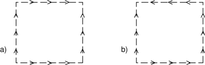
Figure 3: a) Torus formed by identifying opposite edges. b) Klein bottle formed by identification with a twist.

Similarly, the unoriented one-loop open string amplitude comes from the annulus and Möbius strip. We will discuss these amplitudes in more detail later.

The lowest order unoriented amplitude is the projective plane, which is a disk with opposite points identified.

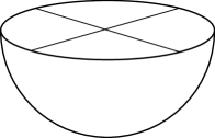
Figure 4: Projective plane formed by identifying opposite points on the disk as shown. This can also be regarded as a sphere with a crosscap inserted.

The projective plane can be thought of as a sphere with a crosscap inserted, where a crosscap is a circular hole with opposite points identified. A sphere with two crosscaps is the same as a Klein bottle; this representation will be useful and will be explained further in section 2.6.

Gauging world-sheet parity is similar to the usual orbifold construction, gauging an internal symmetry of the world-sheet theory. One difference is that there is no direct analog of the twisted states because the Klein bottle does not have the modular transformation $\tau\to-1/\tau$. On the torus, the projection operator implies the insertion of twists in the timelike (vertical) direction of figure 3a; rotating the figure by $90^{\circ}$, these become twists in the spacelike direction, implying twisted states in the spectrum. But if the Klein bottle of figure 3b is rotated by $90^{\circ}$, the directions of time on the two opposite edges do not match and there is no interpretation in terms of intermediate states in this channel.

Various authors have identified open strings as the twisted states of the $\Omega$ projection.[16, 6] There are some definite senses in which these are parallel, but the analogy is not exact and we find it dangerous in that it might lead one to be less than general.

2 Lecture 2: $T$-Duality

2.1 Self-Duality of Closed Strings

For closed strings, let us first study the zero modes. The mode expansion (18) is

$$X^{\mu}(z,{\bar{z}})=x^{\mu}+\tilde{x}^{\mu}-i\sqrt{\alpha^{\prime}\over 2}(\alpha^{\mu}_{0}+{\tilde{\alpha}}^{\mu}_{0})\sigma^{2}+\sqrt{\alpha^{\prime}\over 2}(\alpha^{\mu}_{0}-{\tilde{\alpha}}^{\mu}_{0})\sigma^{1}+{\rm oscillators}.$$ (21)

Noether’s theorem gives the spacetime momentum of a string as

$$p^{\mu}={1\over{\sqrt{2\alpha^{\prime}}}}(\alpha^{\mu}_{0}+{\tilde{\alpha}}^{\mu}_{0}).$$ (22)

Under $\sigma^{1}\to\sigma^{1}+2\pi$, the oscillator term are periodic and $X^{\mu}(z,{\bar{z}})$ changes by $2\pi\sqrt{(\alpha^{\prime}/2)}(\alpha^{\mu}_{0}-{\tilde{\alpha}}^{\mu}_{0}).$ For a non-compact spatial direction $\mu$, $X^{\mu}(z,{\bar{z}})$ is single-valued, and so

$$\alpha^{\mu}_{0}={\tilde{\alpha}}^{\mu}_{0}=\sqrt{\alpha^{\prime}\over 2}p^{\mu}.$$ (23)

Since vertex operators must leave the space (23) invariant, they may contain only the combination $x^{\mu}+\tilde{x}^{\mu}$.

For a compact direction of radius $R$, say $\mu=25$, $X^{25}$ has period $2\pi R$. The momentum $p^{25}$ can take the values $n/R$. Also, under $\sigma^{1}\sim\sigma^{1}+2\pi$, $X^{25}(z,{\bar{z}})$ can change by $2\pi wR$. Thus

$$\alpha^{25}_{0}+{\tilde{\alpha}}^{25}_{0} = {2n\over R}\sqrt{\alpha^{\prime}\over 2}$$

$$\alpha^{25}_{0}-{\tilde{\alpha}}^{25}_{0} = \sqrt{2\over\alpha^{\prime}}wR$$ (24)

and so

$$\alpha^{25}_{0} = \left({n\over R}+{wR\over\alpha^{\prime}}\right)\sqrt{\alpha^{\prime}\over 2}$$

$${\tilde{\alpha}}^{25}_{0} = \left({n\over R}-{wR\over\alpha^{\prime}}\right)\sqrt{\alpha^{\prime}\over 2}.$$ (25)

Turning to the mass spectrum, we have

$$M^{2}\ =\ -p^{\mu}p_{\mu} = {2\over\alpha^{\prime}}(\alpha_{0}^{25})^{2}+{4\over\alpha^{\prime}}({N}-1)$$ (26)

$$= {2\over\alpha^{\prime}}({\tilde{\alpha}}_{0}^{25})^{2}+{4\over\alpha^{\prime}}({\bar{N}}-1).$$

Here $\mu$ runs only over the non-compact dimensions, $N$ is the total level of the left-moving excitations, and $\bar{N}$ the total level of the right-moving excitations. As $R\to\infty$, all states with $w\neq 0$ become infinitely massive, while the $w=0$ states with all values of $n$ go over to a continuum. As $R\to 0$, all states with $n\neq 0$ become infinitely massive. In field theory this is all that would happen—the surviving fields would be independent of the compact coordinate, so the effective dimension is reduced. In closed string theory things work quite differently: the $n=0$ states with all $w$ values form a continuum as $R\to 0$, because it is very cheap to wind around the small circle. In the $R\to 0$ limit, the compactified dimension reappears! This is the first and still most striking indication that strings see spacetime geometry differently from the way we are used to. Indeed, many other examples of ‘stringy geometry’ or ‘quantum geometry’ are closely related to this.[17]

The mass spectra of the theories at radius $R$ and $\alpha^{\prime}/R$ are identical when the winding and Kaluza-Klein modes are interchanged $n\leftrightarrow w$,[18] which takes

$$\alpha^{25}_{0}\rightarrow\alpha^{25}_{0},\quad{\tilde{\alpha}}_{0}^{25}\rightarrow-{\tilde{\alpha}}_{0}^{25}.$$ (27)

The interactions are identical as well.[19] Write the radius-$R$ theory in terms of

$$X^{\prime 25}(z,{\bar{z}})=X^{25}(z)-X^{25}({\bar{z}})\ .$$ (28)

The energy-momentum tensor and OPE and therefore all of the correlation functions are invariant under this rewriting. The only change, evident from eq. (27), is that the zero mode spectrum in the new variable is that of the $\alpha^{\prime}/R$ theory. In other words, these theories are physically identical; $T$-duality, relating the $R$ and $\alpha^{\prime}/R$ theories, is an exact symmetry of perturbative closed string theory. Note that the transformation (28) can be regarded as a spacetime parity transformation acting only on the right-moving degrees of freedom.

This duality transformation is in fact an exact symmetry of closed string theory.[20] To see why, recall from Ooguri’s lectures the appearance of an $SU(2)_{L}\times SU(2)_{R}$ extended gauge symmetry at the self-dual radius. Additional left- and right-moving currents are present at this radius in the massless spectrum,

$$SU(2)_{L}\colon \partial X^{25}(z),\ \ \exp(\pm 2iX^{25}(z)/\sqrt{\alpha^{\prime}})$$

$$SU(2)_{R}\colon \bar{\partial}X^{25}(z),\ \ \exp(\pm 2iX^{25}({\bar{z}})/\sqrt{\alpha^{\prime}})\ .$$ (29)

The marginal operator for the change of radius, $\partial X^{25}{\bar{\partial}}X^{25}$, transforms as a $({\bf 3},{\bf 3})$ and so a rotation by $\pi$ in one of the $SU(2)$’s transforms it into minus itself. The transformation $R\to\alpha^{\prime}/R$ is therefore a ${\bf Z}_{2}$ subgroup of the $SU(2)\times SU(2)$. We may not know what non-perturbative string theory is, but it is a fairly safe bet that it does not violate spacetime gauge symmetries explicitly, else the theory could not be consistent. This is a simple example of an idea which plays a prominent role in the study of string duality: that arguments based on consistency in the low energy field theory place strong constraints on the non-perturbative behavior of strings.

It is important to note that $T$-duality acts nontrivially on the dilaton.[21] By the usual dimensional reduction, the effective 25-dimensional coupling is $e^{\phi}R^{-1/2}$. Duality requires this to be equal to $e^{\phi^{\prime}}R^{\prime-1/2}$, hence

$$e^{\phi^{\prime}}=e^{\phi}R^{-1}{\alpha^{\prime}}^{1/2}.$$ (30)

2.2 $T$-Duality of Open Strings

Now consider the $R\to 0$ limit of the open string spectrum. Open strings cannot wind around the periodic dimension; they have no quantum number comparable to $w$. So when $R\to 0$ the states with nonzero momentum go to infinite mass, but there is no new continuum of states. The behavior is as in field theory: the compactified dimension disappears, leaving a theory in $D-1$ spacetime dimensions. The seeming paradox arises when one remembers that theories with open strings always have closed strings as well, so that in the $R\to 0$ limit the closed strings live in $D$ spacetime dimensions but the open strings only in $D-1$.

One can reason out what is happening as follows. The string in the interior of the open string is the same ‘stuff’ as the closed string is made of, and so should still be vibrating in $D$ dimensions. What distinguishes the open string is its endpoints, and these are restricted to a $D-1$ dimensional hyperplane. Indeed, this follows from the duality transformation (28). The Neumann condition $\partial_{n}X^{25}$ for the original coordinate becomes $\partial_{t}X^{\prime 25}$ for the dual coordinate.[1]${}^{\!-\,}$[8] This is the Dirichlet condition: the $X^{25}$ coordinate of the endpoint is fixed, so the endpoint is constrained to lie on a hyperplane.

In fact, all endpoints are constrained to lie on the same hyperplane. To see this, integrate

$$X^{\prime 25}(\pi)-X^{\prime 25}(0) = \int_{0}^{\pi}d\sigma\partial_{\sigma}X^{\prime 25}\ =\ i\int_{0}^{\pi}d\sigma\partial_{\tau}X^{25}$$ (31)

$$= 2\pi\alpha^{\prime}p^{25}\ =\ \frac{2\pi\alpha^{\prime}n}{R}\ =\ 2\pi nR^{\prime}.$$

That is, $X^{\prime 25}$ at the two ends is equal up to an integral multiple of the periodicity of the dual dimension, corresponding to a string that winds as in figure 5.

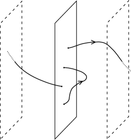
Figure 5: Open strings with endpoints attached to a hyperplane. The dashed planes are periodically identified. The strings shown have winding numbers zero and one.

For two different open strings, consider the connected world-sheet that results from graviton exchange between them. One can carry out the same argument (31) on a path connecting any two endpoints, so all endpoints lie on the same hyperplane. The ends are still free to move in the other $D-2=24$ spatial dimensions.

2.3 $T$-Duality with Chan-Paton Factors and Wilson Lines

Now we study the effect of Chan-Paton factors.[11] Consider the case of $U(N)$, the oriented open string. In compactifying the $X^{25}$ direction, we can include a Wilson line $A_{25}={\rm diag}\{\theta_{1},\theta_{2},\ldots,\theta_{N}\}/2\pi R$, generically breaking $U(N)\to U(1)^{N}$. Locally this is pure gauge,

$$A_{25}=-i\Lambda^{-1}\partial_{25}\Lambda,\qquad\Lambda={\rm diag}\{e^{iX^{25}\theta_{1}/2\pi R},e^{iX^{25}\theta_{2}/2\pi R},\ldots,e^{iX^{25}\theta_{1}/2\pi R}\}\ .$$ (32)

One can then gauge $A_{25}$ away, but the gauge transformation is not periodic and the fields now pick up a phase

$${\rm diag}\left\{e^{-i\theta_{1}},e^{-i\theta_{2}},\ldots,e^{-i\theta_{N}}\right\}$$ (33)

under $X^{25}\to X^{25}+2\pi R$. What is the effect in the dual theory? Due to the phase (33) the open string momenta now in general have fractional parts. Since the momentum is dual to the winding number, we expect the fields in the dual description to have fractional winding number, meaning that their endpoints are no longer on the same hyperplane. Indeed, a string whose endpoints are in the state $|ij\rangle$ picks up a phase $e^{i(\theta_{j}-\theta_{i})}$, so the momentum is $(2\pi n+\theta_{j}-\theta_{i})/2\pi R$. The calculation (31) then gives

$$X^{\prime 25}(\pi)-X^{\prime 25}(0)=(2\pi n+\theta_{j}-\theta_{i})R^{\prime}.$$ (34)

In other words, up to an arbitrary additive normalization, the endpoint in state $i$ is at

$$X^{\prime 25}\ =\ \theta_{i}R^{\prime}\ =\ 2\pi\alpha^{\prime}A_{25,ii}.$$ (35)

There are in general $N$ hyperplanes at different positions as depicted in figure 6.

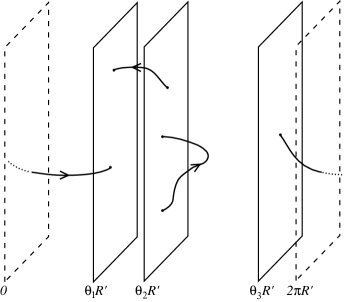
Figure 6: $N=3$ hyperplanes at different positions, with various strings attached.

2.4 D-Brane Dynamics

Let us first note that this whole picture goes through if several coordinates $X^{m}=\{X^{25},X^{24},\ldots,X^{p+1}\}$ are periodic, and we rewrite the periodic dimensions in terms of the dual coordinate. The open string endpoints are then confined to $N$ $(p+1)$-dimensional hyperplanes. The Neumann conditions on the world sheet, $\partial_{n}X^{m}(\sigma^{1},\sigma^{2})=0$, have become Dirichlet conditions $\partial_{t}X^{\prime m}(\sigma^{1},\sigma^{2})=0$ for the dual coordinates.

It is natural to expect that the hyperplane is dynamical rather than rigid.[1] For one thing, this theory still has gravity, and it is difficult to see how a perfectly rigid object could exist. Rather, we would expect that the hyperplanes can fluctuate in shape and position as dynamical objects. We can see this by looking at the massless spectrum of the theory, interpreted in the dual coordinates.

Taking for illustration the case where a single coordinate is dualized, consider the mass spectrum. The $D-1$ dimensional mass is

$$M^{2} = (p^{25})^{2}+{1\over\alpha^{\prime}}({N}-1)$$ (36)

$$= \left({[2\pi n+(\theta_{i}-\theta_{j})]R^{\prime}\over 2\pi\alpha^{\prime}}\right)^{2}+{1\over\alpha^{\prime}}(N-1).$$

Note that $[2\pi n+(\theta_{i}-\theta_{j})]R^{\prime}$ is the minimum length of a string winding between hyperplanes $i$ and $j$. Massless states arise generically only for non-winding open strings whose end points are on the same hyperplane, as the string tension contributes an energy to a stretched string. We have therefore the massless states:

$$\alpha^{\mu}_{-1}|{k};ii\rangle, V=\partial_{t}X^{\mu},$$

$$\alpha^{m}_{-1}|{k};ii\rangle, V=\partial_{t}X^{25}=\partial_{n}X^{\prime 25}.$$ (37)

The first of these is a gauge field living on the hyperplane, with $p+1$ components tangent to the hyperplane. The second was the gauge field in the compact direction in the original theory. In the dual theory it becomes the transverse position of the hyperplane. We have already seen this in eq. (35) for a Wilson line, a constant gauge potential. More general gauge backgrounds would correspond to curved surfaces, and the quanta of the gauge fields to fluctuations. This is the same phenomenon as with spacetime itself. We start with strings in a flat background and discover that a massless closed string state corresponds to fluctuations of the geometry. Here we found first a flat hyperplane, and then discovered that a certain open string state corresponds to fluctuations of its shape.

Thus the hyperplane is indeed a dynamical object, a Dirichlet membrane, or D-brane for short, or more specifically a D $p$-brane. In this terminology, the original Type I theory contains $N$ D 25-branes. A 25-brane fills space, so the string endpoint can be anywhere: it just corresponds to an ordinary Chan-Paton factor.

It is interesting to look at the $U(N)$ symmetry breaking in the dual picture. When no D-branes coincide, there is just one massless vector each, or $U(1)^{N}$ in all, the generic unbroken group. If $m$ D-branes coincide, there are new massless states because strings which are stretched between these branes can achieve vanishing length. Thus, there are $m^{2}$ vectors, forming the adjoint of a $U(m)$ gauge group.[11]${}^{\!,\,}$[22] This coincident position corresponds to $\theta_{1}=\theta_{2}=\cdots=\theta_{m}$ for some subset of the original $\{\theta\}$, so in the original theory the Wilson line left a $U(m)$ subgroup unbroken. At the same time, there appears a set of $m^{2}$ massless scalars: the $m$ positions are promoted to a matrix. This is curious and hard to visualize, but has proven to play an important role in the dynamics of D-branes.[22] Note that if all $N$ branes are coincident, we recover the $U(N)$ gauge symmetry.

This picture seems a bit exotic, and will become more so in the unoriented theory. But all we have done is to rewrite the original open string theory in terms of variables which are more natural in the limit $R\ll\sqrt{\alpha^{\prime}}$. Various puzzling features of the small-radius limit become clear in the $T$-dual picture.

Observe that, since $T$-duality interchanges N and D boundary conditions, a further $T$-duality in a direction tangent to a D $p$-brane reduces it to a $(p-1)$-brane, while a $T$-duality in a direction orthogonal turns it into a $(p+1)$-brane. The case of a nontrivial angle will come up in the next section.

2.5 The D-Brane Action

The world-brane theory consists of a $U(1)$ vector field plus $25-p$ world-brane scalars describing the fluctuations. It is important to consider the low energy effective action for these fields. They are in interaction with the massless closed string fields, whose action was given in the first line of eq. (11). Introduce coordinates $\xi^{a}$, $a=0,\ldots p$ on the brane. The fields on the brane are the embedding $X^{\mu}(\xi)$ and the gauge field $A_{a}(\xi)$. The action is [23]

$$S_{p}=-T_{p}\int d^{p+1}\xi\,e^{-\phi}\det\!^{1/2}\left(G_{ab}+B_{ab}+2\pi\alpha^{\prime}F_{ab}\right)\ ,$$ (38)

where $G_{ab}$ and $B_{ab}$ are the pull-back of the spacetime fields to the brane. All features of this equation can be understood from general reasoning. The $\det\!^{1/2}G_{ab}$ term gives the world-volume. The dilaton dependence $e^{-\phi}=g^{-1}$ arises because this is an open string tree level action.

The dependence on $F$ can be understood as follows.[24]${}^{\!,\,}$[25] Consider a D-brane which is extended in the $X^{1}$ and $X^{2}$ directions, with the other dimensions unspecified, and let there be a constant gauge field $F_{12}$. Go to the gauge $A_{2}=X^{1}F_{12}$. Now $T$-dual along the 2-direction. The open strings then satisfy Dirichlet conditions in this direction, but the relation (35) between the potential and coordinate implies that the D-brane is tilted,

$$X^{\prime 2}=2\pi\alpha^{\prime}X^{1}F_{12}.$$ (39)

This gives a geometric factor in the action,

$$\int dX^{1}\,\sqrt{1+(\partial_{1}X^{\prime 2})^{2}}=\int dX^{1}\,\sqrt{1+(2\pi\alpha^{\prime}F_{12})^{2}}\ .$$ (40)

By boosting the D-brane to be aligned with the coordinate axes and then rotating to bring $F_{ab}$ to block-diagonal form, one can reduce to a product of factors (40) giving $F_{ab}$ in the determinant (38). This determinant is the Born-Infeld action.[26] The combination $B_{ab}+2\pi\alpha^{\prime}F_{ab}$ can be understood as follows. These fields appear in the string world-sheet action as

$$\frac{1}{2\pi\alpha^{\prime}}\int_{\cal M}B+\int_{\partial\cal M}A,$$ (41)

written using differential forms. This is invariant under the vector gauge transformation $\delta A=d\lambda$, but the two-form gauge transformation $\delta B=d\zeta$ gives a surface term that is canceled by assigning a transformation $\delta A=-\zeta/2\pi\alpha^{\prime}$ to the gauge field. Then the combination $B+2\pi\alpha^{\prime}F$ is invariant under both symmetries, and it is this combination that must appear in the action. Thus the form of the action is fully determined.

In the next section we will calculate the value of the tension $T_{p}$, but it is interesting to note that one gets a recursion relation for it from $T$-duality.[27]${}^{\!,\,}$[28] The mass of a D $p$-brane wrapped around a $p$-torus is

$$T_{p}e^{-\phi}\prod_{i=1}^{p}(2\pi R_{i})\ .$$ (42)

Taking the $T$-dual on $X^{p}$ and recalling the transformation (30) of the dilaton, we can rewrite the mass (42) in the dual variables:

$$T_{p}(2\pi\sqrt{{\alpha^{\prime}}})e^{-\phi^{\prime}}\prod_{i=1}^{p-1}(2\pi R_{i})\ =\ T_{p-1}e^{-\phi^{\prime}}\prod_{i=1}^{p-1}(2\pi R_{i})\ ,$$ (43)

or

$$T_{p}=T_{p-1}/2\pi\sqrt{{\alpha^{\prime}}}\ .$$ (44)

For $N$ D-branes the brane fields become matrices as we have seen. Non-derivative terms in the collective coordinates can be deduced by $T$-duality from a constant $A_{a}$ field. The leading action for the latter, from the non-Abelian field strength, is proportional to Tr$([X^{a},X^{b}]\,[X_{a},X_{b}])$. The derivatives are relevant only when this vanishes. The $X_{a}$ then commute and can be diagonalized simultaneously, giving $N$ independent D-branes. The action is therefore

$$S_{p} = -T_{p}\int d^{p+1}\xi\,e^{-\phi}{\rm Tr}\biggl{\{}\det\!^{1/2}\left(G_{ab}+B_{ab}+2\pi\alpha^{\prime}F_{ab}\right)$$ (45)

$$\qquad\qquad\qquad+O([X^{a},X^{b}]^{2})\biggr{\}}\ .$$

The precise form of the commutator term, including coupling to other fields and higher powers of the commutator, can be deduced by $T$-duality from the 26-dimensional non-Abelian Born-Infeld action.

2.6 D-Brane Tension

It is instructive to compute the D-brane tension $T_{p}$, and for the superstring the actual value will be significant. As noted above, it is proportional to $g^{-1}$. One could calculate it from the gravitational coupling to the D-brane, given by the disk with a graviton vertex operator. However, it is much easier to obtain the absolute normalization as follows. Consider two parallel Dirichlet $p$-branes at positions $X^{\prime\mu}=0$ and $X^{\prime\mu}=Y^{\mu}$. These two objects can feel each other‘s presence by exchanging closed strings as shown in figure 7.

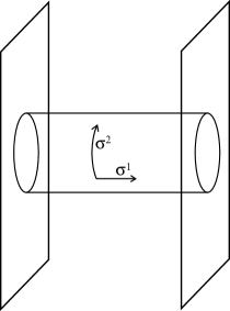
Figure 7: Exchange of a closed string between two D-branes. Equivalently, a vacuum loop of an open string with one end on each D-brane.

This string graph is an annulus, with no vertex operators. It is therefore easily calculated. The poles from graviton and dilaton exchange then give the coupling $T_{p}$ of closed string states to the D-brane.

Parameterize the world-sheet as $(\sigma^{1},\sigma^{2})$ where $\sigma^{2}$ (periodic) runs from $0$ to $2\pi t$, and $\sigma^{1}$ from $0$ to $\pi$. This vacuum graph has the single modulus $t$, running from $0$ to $\infty$. Time-slicing horizontally, so that $\sigma^{2}$ is world-sheet time, gives a loop of open string. Time-slicing vertically instead, so that $\sigma^{1}$ is time, we see a single closed string propagating in the tree channel. The world-line of the open string boundary can be regarded as a vertex connecting the vacuum to the single closed string, i.e., a one-point closed string vertex.[29]${}^{\!,\,}$[30]

Consider the limit $t\to 0$ of the loop amplitude. This is the ultra-violet limit for the open string channel, but unlike the torus, there is no modular group acting to cut off the range of integration. However, because of duality, this limit is correctly interpreted as an infrared limit. Time-slicing vertically shows that the $t\to 0$ limit is dominated by the lowest lying modes in the closed string spectrum. In keeping with string folklore, there are no “ultraviolet limits” of the moduli space which could give rise to high energy divergences. All divergences in loop amplitudes come from pinching handles and are controlled by the lightest states, or the long distance physics.

One loop vacuum amplitudes are given by the Coleman-Weinberg formula, which can be thought of as the sum of the zero point energies of all the modes:[31]

$${\cal A}=V_{p+1}\int\frac{d^{p+1}k}{(2\pi)^{p+1}}\int_{0}^{\infty}{dt\over 2t}\sum_{I}e^{-2\pi\alpha^{\prime}t(k^{2}+M_{I}^{2})}.$$ (46)

Here the sum $I$ is over the physical spectrum of the string, equivalent to the transverse spectrum, and the momentum $k$ is in the $p+1$ extended directions of the D-brane world-sheet. The mass spectrum is given by

$$M^{2}={1\over\alpha^{\prime}}\left(\sum_{n=1}^{\infty}n{\alpha}^{i}_{-n}\alpha_{n}^{i}-1\right)+{Y\cdot Y\over 4\pi^{2}\alpha^{\prime 2}}$$ (47)

where $Y^{m}$ is the separation of the D-branes. The sums over $N_{n}^{i}={\alpha}^{i}_{-n}\alpha_{n}^{i}$ are as usual geometric, giving

$${\cal A}=2V_{p+1}\int_{0}^{\infty}{dt\over 2t}(8\pi^{2}\alpha^{\prime}t)^{-{(p+1)\over 2}}e^{-Y\cdot Yt/2\pi\alpha^{\prime}}f_{1}(q)^{-24}\ .$$ (48)

Here $q=e^{-\pi t}$, the overall factor of 2 is from exchanging the two ends of the string, and we define

$$f_{1}(q) = q^{1/12}\prod_{n=1}^{\infty}(1-q^{2n})$$

$$f_{2}(q) = \sqrt{2}q^{1/12}\prod_{n=1}^{\infty}(1+q^{2n})$$

$$f_{3}(q) = q^{-1/24}\prod_{n=1}^{\infty}(1+q^{2n-1})$$

$$f_{4}(q) = q^{-1/24}\prod_{n=1}^{\infty}(1-q^{2n-1})\ .$$ (49)

We need the asymptotics as $t\to 0$. The asymptotics as $t\to\infty$ are manifest, and the $t\to 0$ asymptotics are then obtained from the modular transformations

$$f_{1}(e^{-{\pi}/{s}})=\sqrt{s}\,f_{1}(e^{-\pi s}),\quad f_{3}(e^{-{\pi}/{s}})=f_{3}(e^{-\pi s}),\quad f_{2}(e^{-{\pi}/{s}})=f_{4}(e^{-\pi s}).$$ (50)

In the present case

$${\cal A}=2V_{p+1}\int_{0}^{\infty}{dt\over 2t}(8\pi^{2}\alpha^{\prime}t)^{-{(p+1)\over 2}}e^{-Y\cdot Yt/2\pi\alpha^{\prime}}t^{12}\left(e^{2\pi/t}+24+\ldots\right).$$ (51)

The leading divergence is from the tachyon and is an uninteresting bosonic artifact. The massless pole, from the second term, is

$${\cal A} \sim V_{p+1}{24\over 2^{12}}(4\pi^{2}\alpha^{\prime})^{11-p}\pi^{(p-23)/2}\Gamma((23-p)/2)|Y|^{p-23}$$ (52)

$$= V_{p+1}{24\pi\over 2^{10}}(4\pi^{2}\alpha^{\prime})^{11-p}G_{25-p}(Y^{2})$$

where $G_{d}(Y^{2})$ is the massless scalar Green’s function in $d$ dimensions.

This can be compared with a field theory calculation, the exchange of graviton plus dilaton between a pair of D-branes. The propagator is from the bulk action (11) and the couplings are from the D-brane action (38). This is a bit of effort because the graviton and dilaton mix, but in the end one finds

$${\cal A}\sim{D-2\over 4}V_{p+1}T_{p}^{2}\kappa_{0}^{2}G_{25-p}(Y^{2})$$ (53)

and so

$$T_{p}={\sqrt{\pi}\over 16\kappa_{0}}(4\pi^{2}\alpha^{\prime})^{(11-p)/2}\ .$$ (54)

This agrees with the recursion relation (44). The actual D-brane tension includes a factor of the dilaton from the action (38),

$$\tau_{p}={\sqrt{\pi}\over 16\kappa}(4\pi^{2}\alpha^{\prime})^{(11-p)/2}\$$ (55)

where $\kappa=\kappa_{0}e^{\phi}$.

As one application, consider $N$ 25-branes, which is the same as an ordinary (fully Neumann) $N$-valued Chan-Paton factor. Expanding the 25-brane Lagrangian (38) to second order in the gauge field gives

$$-{T_{25}\over 4}(2\pi\alpha^{\prime})^{2}e^{-\phi}{\rm Tr}F_{\mu\nu}F^{\mu\nu},$$ (56)

with the trace in the fundamental representation of $U(N)$. This gives the precise numerical relation between the open and closed string couplings.[32]

The asymptotics (51) have an obvious interpretation in terms of a sum over closed string states exchanged between the two D-branes. One can write the cylinder path integral in Hilbert space formalism treating $\sigma_{1}$ rather than $\sigma_{2}$ as time. It then has the form

$$\langle B|e^{-(L_{0}+\tilde{L}_{0})\pi/t}|B\rangle$$ (57)

where the boundary state $|B\rangle$ is the closed string state created by the boundary loop. We will not have time to develop this formalism but it is useful in finding the couplings between closed and open strings.[29]${}^{\!,\,}$[30]

2.7 Unoriented Strings and Orientifolds.

The $R\to 0$ limit of an unoriented theory also leads to new objects. The effect of $T$-duality can easily be understood by viewing it as a one-sided parity transformation. For closed strings, the original coordinate is $X^{m}(z,{\bar{z}})=X^{m}(z)+X^{m}({\bar{z}})$ and the dual is $X^{\prime m}(z,{\bar{z}})=X^{m}(z)-X^{m}({\bar{z}})$. The action of world sheet parity reversal is to exchange $X^{\mu}(z)$ and $X^{\mu}({\bar{z}})$. In terms of the dual coordinate this is

$$X^{\prime m}(z,{\bar{z}})\leftrightarrow-X^{\prime m}({\bar{z}},z),$$ (58)

which is the product of a world-sheet and a spacetime parity operation. In the unoriented theory, strings are invariant under the action of $\Omega$, so in the dual theory we have gauged the product of world-sheet parity with a spacetime symmetry, here parity. This generalization of the usual unoriented theory is known as an orientifold, a play on the term orbifold for gauging a discrete spacetime symmetry.

Separate the string wavefunction into its internal part and its dependence on the center of mass $x^{m}$, and take the internal wavefunction to be an eigenstate of $\Omega$. The projection then determines the string wavefunction at $-x^{m}$ to be the same as at $x^{m}$, up to a sign. For example, the various components of the metric and antisymmetric tensor satisfy

$$G_{\mu\nu}(x^{\mu},-x^{m})=G_{\mu\nu}(x^{\mu},x^{m}), B_{\mu\nu}(x^{\mu},-x^{m})=-B_{\mu\nu}(x^{\mu},x^{m}),$$

$$G_{\mu n}(x^{\mu},-x^{m})=-G_{\mu n}(x^{\mu},x^{m}), B_{\mu n}(x^{\mu},-x^{m})=B_{\mu n}(x^{\mu},x^{m}),$$

$$G_{mn}(x^{\mu},-x^{m})=G_{mn}(x^{\mu},x^{m}), B_{mn}(x^{\mu},-x^{m})=-B_{mn}(x^{\mu},x^{m})\ .$$ (59)

In other words, the $T$-dual spacetime is the torus $T^{25-p}$ modded by a ${\bf Z}_{2}$ reflection in the compact directions. This is the same as the orbifold construction, the only difference being the extra sign. In the case of a single periodic dimension, for example, the dual spacetime is the line segment $0\leq x^{25}\leq\pi R^{\prime}$, with orientifold fixed planes at the ends. It should be noted that orientifold planes are not dynamical. Unlike the case of D-branes, there are no string modes tied to the orientifold plane to represent fluctuations in its shape.

Notice also that away from the orientifold fixed planes, the local physics is that of the oriented string theory. Unlike the original unoriented theory, where the projection removes half the states locally, here it relates the amplitude to find a string at some point to the amplitude to find it at the image point.

The orientifold construction was discovered via $T$-duality [1] and independently from other points of view.[16]${}^{\!,\,}$[6] One can of course consider more general orientifolds which are not simply $T$-duals of toroidal compactifications. There have been quite a few papers on orientifolds and their various duals. This will not be a primary focus of these lectures—we will be interested in orientifolds mainly insofar as they arise in understanding the physics of D-branes.

In the case of open strings, the situation is similar. Let us focus for convenience on a single compact dimension. Again there is one orientifold fixed plane at $0$ and another at $\pi R^{\prime}$. Introducing $SO(N)$ Chan-Paton factors, a Wilson line can be brought to the form

$${\rm diag}\{\theta_{1},-\theta_{1},\theta_{2},-\theta_{2},\cdots,\theta_{N/2},-\theta_{N/2}\}.$$ (61)

Thus in the dual picture there are ${1\over 2}N$ D-branes on the line segment $0\leq X^{\prime 25}<\pi R^{\prime}$, and ${1\over 2}N$ at their image points under the orientifold identification. Strings can stretch between D-branes and their images as shown.

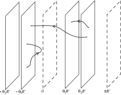
Figure 8: Orientifold planes at $0$ and $\pi R^{\prime}$, D-branes at $\theta_{1}R^{\prime}$ and $\theta_{2}R^{\prime}$, and D-brane images at -$\theta_{1}R^{\prime}$ and $-\theta_{2}R^{\prime}$. The twist operator $\Omega$ acts on any string by a combination of a spacetime reflection and reversing the orientation arrow.

The generic gauge group is $U(1)^{N/2}$. As in the oriented case, if $m$ D-branes are coincident there is a $U(m)$ gauge group. But now if the $m$ D-branes in addition lie at one of the fixed planes, then strings stretching between one of these branes and one of the image branes also become massless and we have the right spectrum of additional states to fill out $SO(2m)$. The maximal $SO(N)$ is restored if all of the branes are coincident at a single orientifold plane. Note that this maximally symmetric case is asymmetric between the two fixed planes. Similar considerations apply to $USp(N)$.

We should emphasize that there are $\frac{1}{2}N$ dynamical D-branes but an $N$-valued Chan-Paton index. An interesting case is when $m+\frac{1}{2}$ D-branes lie on a fixed plane, which makes sense because the number $2m+1$ of indices is integer. A brane plus image can move away from the fixed plane, but the number of branes remaining is always half-integer.

The orientifold plane, like the D-brane, couples to the dilaton and metric. The amplitude is the same as in the previous section, but with $RP^{2}$ in place of the disk; that is, a crosscap replaces the boundary loop. The orientifold identifies $X^{m}$ with $-X^{m}$ at the opposite point on the crosscap, so the crosscap is localized near one of the orientifold fixed planes. Again the easiest way to calculate this is via vacuum graphs, the cylinder with one or both boundary loops replaced by crosscaps. These give the Möbius strip and Klein bottle, respectively.

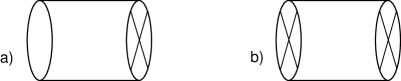
Figure 9: a) Möbius strip as cylinder with crosscap at one end. b) Klein bottle as cylinder with crosscaps at each end.

To understand this, consider figure 10, which shows two copies of the fundamental region for the Möbius strip.

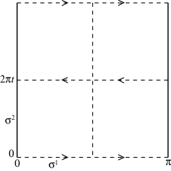
Figure 10: Two copies of the fundamental region for the Möbius strip.

The lower half is identified with the reflection of the upper, and the edges $\sigma^{1}=0,\pi$ are boundaries. Taking the lower half as the fundamental region gives the familiar representation of the Möbius strip as a strip of length $2\pi t$, with ends twisted and glued. Taking instead the left half of the figure, the line $\sigma^{1}=0$ is a boundary loop while the line $\sigma^{1}=\pi/2$ is identified with itself under a shift $\sigma^{2}\to\sigma^{2}+2\pi t$ plus reflection of $\sigma^{1}$: it is a crosscap. The same construction applies to the Klein bottle, with the right and left edges now identified.

The Möbius strip is given by the vacuum amplitude

$${\cal A}_{\rm M}=V_{p+1}\int\frac{d^{p+1}k}{(2\pi)^{p+1}}\int_{0}^{\infty}{dt\over 2t}\sum_{I}{\Omega_{i}\over 2}e^{-2\pi\alpha^{\prime}t(p^{2}+M_{I}^{2})},$$ (62)

where $\Omega_{I}$ is the $\Omega$ eigenvalue of state $i$. The oscillator contribution to $\Omega_{I}$ is $(-1)^{N}$ from eq. (13). For the $SO(N)$ open string the Chan-Paton factors have ${1\over 2}N(N+1)$ even states and ${1\over 2}N(N-1)$ odd for a net of $+N$. For $USp(N)$ these numbers are reversed for a net of $-N$. Focus on a D-brane and its image, which correspondingly contribute $\pm 2$. The diagonal elements, which contribute to the trace, are those where one end is on the D-brane and one on its image. The total separation is then $Y^{m}=2X^{m}$. Then,

$${\cal A}_{\rm M} = \pm V_{p+1}\int_{0}^{\infty}{dt\over 2t}(8\pi^{2}\alpha^{\prime}t)^{-{(p+1)\over 2}}e^{-2X\cdot Xt/\pi\alpha^{\prime}}$$ (63)

$$\qquad\qquad\qquad\qquad\qquad\left[q^{-2}\prod_{k=1}^{\infty}(1+q^{4k-2})^{-24}(1-q^{4k})^{-24}\right]$$

The factor in braces $[\ ]$ is

$$f_{3}(q^{2})^{-24}f_{1}(q^{2})^{-24} = (2t)^{12}f_{3}(e^{-\pi/2t})^{-24}f_{1}(e^{-\pi/2t})^{-24}$$ (64)

$$= (2t)^{12}\left(e^{\pi/2t}-24+\ldots\right)\ .$$

One thus finds a pole

$$\mp 2^{p-12}V_{p+1}{3\pi\over 2^{6}}(4\pi^{2}\alpha^{\prime})^{11-p}G_{25-p}(X^{2})\ .$$ (65)

This is to be compared with the field theory result ${D-2\over 2}V_{p+1}T_{p}T^{\prime}_{p}\kappa_{0}^{2}G_{25-p}(Y^{2})$, where $T^{\prime}_{p}$ is the fixed-plane tension. A factor of 2 as compared to the earlier field theory calculation (53) comes because the spacetime boundary forces all the flux in one direction. Thus the fixed-plane and D-brane tensions are related

$$\tau^{\prime}_{p}=\mp 2^{p-13}\tau_{p}.$$ (66)

A similar calculation with the Klein bottle gives a result proportional to $\tau_{p}^{\prime 2}$.

Noting that there are $2^{25-p}$ fixed planes, the total fixed-plane source is $\mp 2^{12}\tau_{p}$. The total source must vanish because the volume is finite and there is no place for flux to go. Thus there are $2^{12}$ D-branes (times two for the images) and the group is $SO(2^{13})=SO(2^{D/2})$.[33] For this group the dilaton and graviton tadpoles cancel at order $g^{-1}$. This has no special significance in the bosonic string, as the one loop $g^{0}$ tadpoles are nonzero and imaginary due to the tachyon instability, but similar boundary combinatorics will give a restriction on anomaly free Chan-Paton gauge groups in the superstring.

3 Lecture 3: Superstrings and $T$-Duality

3.1 Open Superstrings

All of the exotic phenomena that we found in the bosonic string will appear in the superstring as well, together with some important new ingredients. We first review open and unoriented superstrings.

The superstring world-sheet action is

$$S={{1}\over{4\pi}}\int_{\cal M}d^{2}\sigma\{\alpha^{\prime-1}\partial X^{\mu}\bar{\partial}X_{\mu}+\psi^{\mu}\bar{\partial}\psi_{\mu}+\tilde{\psi}^{\mu}\partial\tilde{\psi}_{\mu}\}$$ (67)

where the open string world-sheet is the strip $0<\sigma^{1}<\pi$, $-\infty<\sigma^{2}<\infty$. The condition that the surface term in the equation of motion vanishes allows two possible Lorentz invariant boundary conditions on world-sheet fermions:

$${\rm R\colon} \psi^{\mu}(0,\sigma^{2})=\tilde{\psi^{\mu}}(0,\sigma^{2})\qquad\psi^{\mu}(\pi,\sigma^{2})=\tilde{\psi^{\mu}}(\pi,\sigma^{2})$$

$${\rm NS\colon} \psi^{\mu}(0,\sigma^{2})=-\tilde{\psi^{\mu}}(0,\sigma^{2})\qquad\psi^{\mu}(\pi,\sigma^{2})=\tilde{\psi^{\mu}}(\pi,\sigma^{2})$$ (68)

We can always take the boundary condition at one end, say $\sigma^{1}=\pi$, to have a $+$ sign by redefinition of $\tilde{\psi}$. The boundary conditions and equations of motion are conveniently summarized by the doubling trick, taking just left-moving (analytic) fields $\psi^{\mu}$ on the range $0$ to $2\pi$ and defining $\tilde{\psi}^{\mu}(\sigma^{1},\sigma^{2})$ to be $\psi^{\mu}(2\pi-\sigma^{1},\sigma^{2})$. These left-moving fields are periodic in the Ramond (R) sector and antiperiodic in the Neveu-Schwarz (NS).

In the NS sector the fermionic oscillators are half-integer moded, giving a ground state energy of $(-{{8}\over{24}})+(-{{8}\over{48}})=-{1\over 2}$ from the eight transverse coordinates and eight transverse fermions. The ground state is a Lorentz singlet and has odd fermion number, $(-1)^{F}=-1$. This assignment is necessary in order for $(-1)^{F}$ to be multiplicatively conserved. The GSO projection, onto states with even fermion number, removes the open string tachyon from the superstring spectrum. Massless particle states in ten dimensions are classified by their $SO(8)$ representation under Lorentz rotations that leave the momentum invariant. The lowest lying states in the NS sector are the eight transverse polarizations of the massless open string photon, $A^{\mu}$,

$$\psi^{\mu}_{-1/2}|{k}\rangle,\qquad M^{2}={{1}\over{\alpha^{\prime}}}(N-{\textstyle{1\over 2}})$$ (69)

forming the vector of $SO(8)$.

The fermionic oscillators in the Ramond sector are integer-moded. In the R sector the ground state energy always vanishes because the world-sheet bosons and their superconformal partners have the same moding. The Ramond vacuum is degenerate, since the $\psi^{\mu}_{0}$ take ground states into ground states, so the latter form a representation of the ten-dimensional Dirac matrix algebra

$$\{\psi^{\mu}_{0},\psi^{\nu}_{0}\}=\eta^{\mu\nu}\ .$$ (70)

The following basis for this representation is often convenient. Form the combinations

$$d^{\pm}_{i} = {{1}\over{\sqrt{2}}}\left(\psi^{2i}_{0}\pm i\psi^{2i+1}_{0}\right)\qquad i=1,\cdots,4$$

$$d^{\pm}_{0} = {{1}\over{\sqrt{2}}}\left(\psi^{1}_{0}\mp\psi^{0}_{0}\right)$$ (71)

In this basis, the Clifford algebra takes the form

$$\{d^{+}_{i},d^{-}_{j}\}=\delta_{ij}\ .$$ (72)

The $d^{\pm}_{i}$, $i=0,\cdots,4$ act as raising and lowering operators, generating the 32 Ramond ground states. Denote these states

$$|s_{0},s_{1},s_{2},s_{3},s_{4}\rangle=|{\bf s}\rangle$$ (73)

where each of the $s_{i}$ is $\pm{\textstyle{1\over 2}}$, and where

$$d^{-}_{i}|-{\textstyle{1\over 2}},-{\textstyle{1\over 2}},-{\textstyle{1\over 2}},-{\textstyle{1\over 2}},-{\textstyle{1\over 2}}\rangle=0$$ (74)

while $d^{+}_{i}$ raises $s_{i}$ from $-{\textstyle{1\over 2}}$ to ${\textstyle{1\over 2}}$. The significance of this notation is as follows. The fermionic part of the ten-dimensional Lorentz generators is

$$S^{\mu\nu}=-{{i}\over{2}}\sum_{r\in{\bf Z}+\kappa}\psi^{[\mu}_{-r}\psi^{\nu]}_{r}$$ (75)

where $\kappa=0$ (${\textstyle{1\over 2}}$) in the R (NS) sector. The states above are eigenstates of $S_{0}=iS^{01}$, $S_{i}=S^{2i,2i+1}$, with $s_{i}$ the corresponding eigenvalues. Since the Lorentz generators always flip an even number of $s_{i}$, the Dirac representation $\bf 32$ decomposes into a $\bf 16$ with an even number of $-{\textstyle{1\over 2}}$’s and $\bf 16^{\prime}$ with an odd number.

Physical states are annihilated by the zero mode of the supersymmetry generator, which on the ground states reduces to $G_{0}=p_{\mu}\psi^{\mu}_{0}$. In the frame $p^{0}=p^{1}$ this becomes $s_{0}={\textstyle{1\over 2}}$, giving a sixteen-fold degeneracy for the physical Ramond vacuum. This is a representation of $SO(8)$ which again decomposes into ${\bf 8_{s}}$ with an even number of $-{\textstyle{1\over 2}}$’s and ${\bf 8_{c}}$ with an odd number.

The GSO projection keeps one irreducible representation; the two choices, $\bf 16$ or $\bf 16^{\prime}$, are physically equivalent, differing only by a spacetime parity redefinition. It is useful to think of the GSO projection in terms of locality of the OPE of a general vertex operator with the gravitino vertex operator. Suppose we take a projection which includes the operator $e^{-\phi/2+i(H_{0}+H_{1}+H_{2}+H_{3}+H_{4})/2}$, where the $H_{i}$ are the bosonization of $\psi^{\mu}$.[34] In the NS sector this has a branch cut with the ground state vertex operator $e^{-\phi}$, accounting for the sign discussed in footnote 6 for the $-1$ picture vertex operator. In the R sector the ghost plus longitudinal part of the OPE is local, so we have

$$\sum_{i=1}^{4}s_{i}=0\pmod{2},$$ (76)

picking out the ${\bf 8_{s}}$.

The ground state spectrum is then ${\bf 8}_{v}\oplus{\bf 8}_{s}$, a vector multiplet of $D=10$, $N=1$ spacetime supersymmetry. Including Chan-Paton factors gives again a $U(N)$ gauge theory in the oriented theory and $SO(N)$ or $USp(N)$ in the unoriented.

3.2 Closed Superstrings

The closed string spectrum is the product of two copies of the open string spectrum, with right- and left-moving levels matched. In the open string the two choices for the GSO projection were equivalent, but in the closed string there are two inequivalent choices, taking the same (IIB) or opposite (IIA) projections on the two sides. These lead to the massless sectors

$${\rm Type~{}IIA\colon} ({\bf 8_{v}}\oplus{\bf 8_{s}})\otimes({\bf 8_{v}}\oplus{\bf 8_{c}})$$

$${\rm Type~{}IIB\colon} ({\bf 8_{v}}\oplus{\bf 8_{s}})\otimes({\bf 8_{v}}\oplus{\bf 8_{s}})$$ (77)

of $SO(8)$.

The various products are as follows. In the NS-NS sector, this is

$${\bf 8_{v}}\otimes{\bf 8_{v}}=\phi\oplus B_{\mu\nu}\oplus G_{\mu\nu}={\bf 1}\oplus{\bf 28}\oplus{\bf 35}.$$ (78)

In the R-R sector, the IIA and IIB spectra are respectively

$${\bf 8_{s}}\otimes{\bf 8_{c}} = [1]\oplus[3]={\bf 8_{v}}\oplus{\bf 56_{t}}$$

$${\bf 8_{s}}\otimes{\bf 8_{s}} = [0]\oplus[2]\oplus[4]_{+}={\bf 1}\oplus{\bf 28}\oplus{\bf 35}_{+}.$$ (79)

Here $[n]$ denotes the $n$-times antisymmetrized representation of $SO(8)$, with $[4]_{+}$ being self-dual. Note that the representations $[n]$ and $[8-n]$ are the same, being related by contraction with the 8-dimensional $\epsilon$-tensor. The NS-NS and R-R spectra together form the bosonic components of $D=10$ IIA (nonchiral) and IIB (chiral) supergravity respectively. In the NS-R and R-NS sectors are the products

$${\bf 8_{v}}\otimes{\bf 8_{c}} = {\bf 8_{s}}\oplus{\bf 56_{c}}$$

$${\bf 8_{v}}\otimes{\bf 8_{s}} = {\bf 8_{c}}\oplus{\bf 56_{s}}.$$ (80)

The $\bf 56_{s,c}$ are gravitinos, their vertex operators having one vector and one spinor index. They must couple to conserved spacetime supercurrents. In the IIA theory the two gravitinos (and supercharges) have opposite chirality, and in the IIB the same.

Let us develop further the vertex operators for the R-R states. This will involve a product of spin fields,[34] $e^{-{{\varphi}\over{2}}-{{\tilde{\varphi}}\over{2}}}S_{\alpha}\tilde{S}_{\beta}$. These again decompose into antisymmetric tensors, now of $SO(9,1)$:

$$V=e^{-{{\varphi}\over{2}}-{{\tilde{\varphi}}\over{2}}}S_{\alpha}\tilde{S}_{\beta}(\Gamma^{[\mu_{1}}\cdots\Gamma^{\mu_{n}]}C)_{\alpha\beta}G_{[\mu_{1}\cdots\mu_{n}]}(X)$$ (81)

with $C$ the charge conjugation matrix. In the IIA theory the product is ${\bf 16}\otimes{\bf 16^{\prime}}$ giving even $n$ (with $n\cong 10-n$) and in the IIB theory it is ${\bf 16}\otimes{\bf 16}$ giving odd $n$. As is usual, the classical equations of motion follow from the physical state conditions, which at the massless level reduce to $G_{0}\cdot V=\tilde{G}_{0}\cdot V=0.$ The relevant part of $G_{0}$ is just $p_{\mu}\psi^{\mu}_{0}$ and similarly for $\tilde{G}_{0}$. The $p_{\mu}$ acts by differentiation on $G$, while $\psi_{0}^{\mu}$ acts on the spin fields as it does on the corresponding ground states: as multiplication by $\Gamma^{\mu}$. Noting the identity

$$\Gamma^{\nu}\Gamma^{[\mu_{1}}\cdots\Gamma^{\mu_{n}]}=\Gamma^{[\nu}\cdots\Gamma^{\mu_{n}]}+\left(\delta^{\nu\mu_{1}}\Gamma^{[\mu_{2}}\cdots\Gamma^{\mu_{n}]}+{\rm perms}\right)$$ (82)

and similarly for right multiplication, the physical state conditions become

$$dG=0\qquad\qquad d{}^{*}G=0.$$ (83)

These are the Bianchi identity and field equation for an antisymmetric tensor field strength. This is in accord with the representations found: in the IIA theory we have odd-rank tensors of $SO(8)$ but even-rank tensors of $SO(9,1)$ (and reversed in the IIB), the extra index being contracted with the momentum to form the field strength. It also follows that R-R amplitudes involving elementary strings vanish at zero momentum, so strings do not carry R-R charges.

As an aside, when the dilaton background is nontrivial, the Ramond generators have a term $\phi_{,\mu}\partial\psi^{\mu}$, and the Bianchi identity and field strength pick up terms proportional to $d\phi\wedge G$ and $d\phi\wedge{}^{*}G$. The Bianchi identity is nonstandard, so $G$ is not of the form $dC$. Defining $G^{\prime}=e^{-\phi}G$ removes the extra term from both the Bianchi identity and field strength. The field $G^{\prime}$ is thus decoupled from the dilaton. In terms of the action, the fields $G$ in the vertex operators appear with the usual closed string $e^{-2\phi}$ but with non-standard dilaton gradient terms. The fields we are calling $G^{\prime}$ (which in fact are the usual fields used in the literature) have a dilaton-independent action.

The IIB theory is invariant under world-sheet parity, so we can again form an unoriented theory by gauging. Projecting onto $\Omega=+1$ interchanges left-moving and right-moving oscillators and so one linear combination of the R-NS and NS-R gravitinos survives, leaving $D=10$, $N=1$ supergravity. In the NS-NS sector, the dilaton and graviton are symmetric under $\Omega$ and survive, while the antisymmetric tensor is odd and is projected out. In the R-R sector, it is clear by counting that the $\bf 1$ and ${\bf 35}_{+}$ are in the symmetric product of ${\bf 8_{s}}\otimes{\bf 8_{s}}$ while the $\bf 28$ is in the antisymmetric. The R-R vertex operator is the product of right- and left-moving fermions, so there is an extra minus in the exchange and it is the $\bf 28$ that survives. The bosonic massless sector is thus ${\bf 1}\oplus{\bf 28}\oplus{\bf 35}$, the $D=10$ $N=1$ supergravity multiplet. This is the same multiplet as in the heterotic string, but now the antisymmetric tensor is from the R-R sector.

The open superstring has only $N=1$ supersymmetry. In order that the closed strings couple consistently they must also have $N=1$ supergravity and so the theory must be unoriented. In fact, spacetime anomaly cancellation implies that the only consistent $N=1$ superstring is the $SO(32)$ open plus closed string theory. Now, as a general principle any such inconsistency in the low energy theory should be related to some stringy inconsistency. This is the case, but it will be more convenient to discuss this later after some discussion of $T$-duality.

3.3 $T$-Duality of Type II Superstrings

Even in the closed oriented Type II theories $T$-duality has an interesting effect.[20]${}^{\!,\,}$[1]. Consider compactifying a single coordinate $X^{9}$. In the $R\to\infty$ limit the momenta are $p^{9}_{R}=p^{9}_{L}$, while in the $R\to 0$ limit $p^{9}_{R}=-p^{9}_{L}$. Both theories are $SO(9,1)$ invariant but under different $SO(9,1)$’s. Duality reverses the sign of the right-moving $X^{9}({\bar{z}})$; therefore by superconformal invariance it does so on $\tilde{\psi}^{9}({\bar{z}})$. Separate the Lorentz generators into their left-and right-moving parts $M^{\mu\nu}+\tilde{M}^{\mu\nu}$. Duality reverses all terms in $\tilde{M}^{\mu 9}$, so the $\mu 9$ Lorentz generators of the $T$-dual theory are $M^{\mu 9}-\tilde{M}^{\mu 9}$. In particular this reverses the sign of the helicity $\tilde{s}_{4}$ and so switches the chirality on the right-moving side. If one starts in the IIA theory, with opposite chiralities, the $R\to 0$ theory has the same chirality on both sides and is the $R\to\infty$ limit of the IIB theory, and vice versa. More simply put, duality is a one-sided spacetime parity operation and so reverses the relative chiralities of the right- and left-moving ground states. The same is true if one dualizes on any odd number of dimensions, while dualizing on an even number returns the original Type II theory.

Since the IIA and IIB theories have different R-R fields, $T_{9}$ duality must transform one set into the other. The action of duality on the spin fields is of the form

$$S_{\alpha}(z)\to S_{\alpha}(z),\qquad\tilde{S}_{\alpha}(\bar{z})\to P_{9}\tilde{S}_{\alpha}(\bar{z})$$ (84)

for some matrix $P_{9}$, the parity transformation (9-reflection) on the spinors. In order for this to be consistent with the action $\tilde{\psi}^{9}\to-\tilde{\psi}^{9}$, $P_{9}$ must anticommute with $\Gamma^{9}$ and commute with the remaining $\Gamma^{\mu}$. Thus $P_{9}=\Gamma^{9}\Gamma^{11}$ (the phase of $P_{9}$ is determined, up to sign, by hermiticity of the spin field). Now consider the effect on the R-R vertex operators (81). The $\Gamma^{11}$ just contributes a sign, because the spin fields have definite chirality. Then by the $\Gamma$-matrix identity (82), the effect is to add a 9-index to $G$ if none is present, or to remove one if it is. The effect on the potential $C$ ($G=dC$) is the same. Take as an example the Type IIA vector $C_{\mu}$. The component $C_{9}$ maps to the IIB scalar $C$, while the $\mu\neq 9$ components map to $C_{\mu 9}$. The remaining components of $C_{\mu\nu}$ come from $C_{\mu\nu 9}$, and so on.

3.4 $T$-Duality of Type I Superstrings

The action of $T$-duality in the open and unoriented Type I theory produces D-branes and orientifold planes, just as in the bosonic string. Let us focus here on a single D-brane, taking a limit in which the other D-branes and the orientifold planes are distant and can be ignored. Away from the D-brane, only closed strings propagate. The local physics is that of the Type II theory, with two gravitinos. This is true even if though we began with the unoriented Type I theory which has only a single gravitino. The point is that the closed string begins with two gravitinos, one with the spacetime supersymmetry on the right-moving side of the world-sheet and one on the left. The orientation projection of the Type I theory leaves one linear combination of these. But in the $T$-dual theory, the orientation projection does not constrain the local state of the string, but relates it to the state of the (distant) image gravitino. Locally there are two independent gravitinos, with equal chiralities if an even number of dimensions have been dualized and opposite if an odd number.

However, the open string boundary conditions are invariant under only one supersymmetry. In the original Type I theory, the left-moving world-sheet current for spacetime supersymmetry $j_{\alpha}(z)$ flows into the boundary and the right-moving current $\tilde{j}_{\alpha}(\bar{z})$ flows out, so only the total charge $Q_{\alpha}+\tilde{Q}_{\alpha}$ of the left- and right-movers is conserved. Under $T$-duality this becomes

$$Q_{\alpha}+\left({\textstyle\prod_{m}}P_{m}\right)\tilde{Q}_{\alpha}\ ,$$ (85)

where the product of reflections $P_{m}$ runs over all the dualized dimensions, that is, over all directions orthogonal to the D-brane. Closed strings couple to open, so the general amplitude has only one linearly realized supersymmetry. That is, the vacuum without D-branes is invariant under $N=2$ supersymmetry, but the state containing the D-brane is invariant under only $N=1$: it is a BPS state.[2]${}^{\!,\,}$[13]

BPS states must carry conserved charges. In the present case there is only one set of charges with the correct Lorentz properties, namely the antisymmetric R-R charges. The world volume of a $p$-brane naturally couples to a ($p+1$)-form potential $C_{(p+1)}$, which has a ($p+2$)-form field strength $G_{(p+2)}$. This identification can also be made from the $g^{-1}$ behavior of the D-brane tension: this is the behavior of an R-R soliton.[35]${}^{\!-\,}$[39], as will be developed further in section 5.8.

The IIA theory has $p=0$, 2, 4, 6, and 8-branes. The vertex operators (81) describe field strengths of all even ranks from 0 to 10. By a $\Gamma$-matrix identity the $n$-form and $(10-n)$-form field strengths are Hodge dual to one another, so a $p$-brane and $(6-p)$-brane are sources for the same field, but one ‘magnetic’ and one ‘electric.’ The field equation for the 10-form field strength allows no propagating states, but the field can still have a physically significant energy density [2]${}^{\!,\,}$[40]${}^{\!-\,}$[41]. Curiously, the 0-form field strength should couple to a $(-2)$-brane, but it is not clear how to interpret this—perhaps there is something interesting to learn here.

The IIB theory has $p=-1$, 1, 3, 5, 7, and 9-branes. The vertex operators (81) describe field strengths of all odd ranks from 1 to 9, appropriate to couple to all but the 9-brane. The 9-brane does couple to a nontrivial potential, as we will see below.

A $(-1)$-brane is a Dirichlet instanton, defined by Dirichlet conditions in the time direction as well as all spatial directions.[10] Of course, it is not clear that $T$-duality in the time direction has any meaning, but one can argue for the presence of $(-1)$-branes as follows. Given $0$-branes in the IIA theory, there should be virtual $0$-brane world-lines that wind in a purely spatial direction. Such world-lines are required by quantum mechanics, but note that they are essentially instantons, being localized in time. A $T$-duality in the winding direction then gives a $(-1)$-brane. One of the first clues to the relevance of D-branes [11] was the observation that D-instantons, having action $g^{-1}$, would contribute effects of order $e^{-1/g}$ as expected from the behavior of large orders of string perturbation theory.[12]

3.5 The D-Brane Action and Charge

We have concluded that the D-brane must couple to a ($p+1$)-form potential. The spacetime plus D-brane action then includes

$$S={1\over 2}\int G_{(p+2)}{}^{*}G_{(p+2)}+i\mu_{p}\int_{p-\rm brane}C_{(p+1)},$$ (86)

where the ($p+1$)-form charge of the D $p$-brane is denoted $\mu_{p}$. As discussed earlier, the dilaton does not appear in the action. However, there are additional terms involving the D-brane gauge field, similar to the Born-Infeld terms. Again these can be determined from $T$-duality. Consider, as an example, a 1-brane in the 1-2 plane. The action is

$$\int dx^{1}\,\left(C_{1}+\partial_{1}X^{2}C_{2}\right)\ .$$ (87)

Under a $T$-duality in the 2-direction this becomes

$$\int dx^{1}\,\left(C_{12}+2\pi\alpha^{\prime}F_{12}C\right)\ .$$ (88)

We have used the $T$-transformation of the $C$ fields as discussed in section 3.3. This argument is easily generalized, with the Chern-Simons-like result

$$i\mu_{p}\int_{p-\rm brane}{\rm Tr}\left(e^{2\pi\alpha^{\prime}F+B}\right)\textstyle{\sum}_{p}C_{(p+1)}\ .$$ (89)

The expansion of the integrand (89) involves forms of various rank; the integral picks out precisely the terms that are proportional to the volume form of the $p$-brane.[42]${}^{\!-\,}$[43]${}^{\!,\,}$[25]${}^{\!,\,}$[27] There are also couplings of the R-R potentials to curvature.[44]${}^{\!,\,}$[45] In addition, the coupling of the D-brane to NS-NS and open string states has the same form (38) as the bosonic D-brane theory.

The D-brane, unlike the fundamental string, carries R-R charge. It is interesting to see how this is consistent with our earlier discussion of string vertex operators.[46] The R-R vertex operator (81) is in the $(-{\textstyle{1\over 2}},-{\textstyle{1\over 2}})$ picture, which can be used in almost all processes. In the disk, however, the total right+left ghost number must be $-2$. With two or more R-R vertex operators, all can be in the $(-{\textstyle{1\over 2}},-{\textstyle{1\over 2}})$ picture (with picture changing operators included as well), but a single vertex operator must be in either the $(-{3\over 2},-{\textstyle{1\over 2}})$ or the $(-{\textstyle{1\over 2}},-{3\over 2})$ picture. The $(-{\textstyle{1\over 2}},-{\textstyle{1\over 2}})$ vertex operator is essentially $e^{-\varphi}G_{0}$ times the $(-{3\over 2},-{\textstyle{1\over 2}})$ operator, so besides the shift in the ghost number the latter has one less power of momentum and one less $\Gamma$-matrix. The missing factor of momentum turns $G$ into $C$, and the missing $\Gamma$-matrix gives the correct Lorentz representations for the potential rather than the field strength.

To obtain the D-brane tension and R-R charge, one can consider the same vacuum cylinder as in the bosonic string.[2] Carrying out the traces over the open superstring spectrum gives

$$A = 2V_{p+1}\int{dt\over 2t}\,(8\pi^{2}\alpha^{\prime}t)^{-(p+1)/2}e^{-t{Y^{2}\over 2\pi\alpha^{\prime}}}$$ (90)

$$\qquad\qquad\qquad\qquad\qquad\frac{-f_{2}(q)^{8}+f_{3}(q)^{8}-f_{4}(q)^{8}}{2f_{1}^{8}(q)},$$

where again $q=e^{-\pi t}$. The three terms in the fraction come from the open string R sector with ${1\over 2}$ in the trace, from the NS sector with ${1\over 2}$ in the trace, and the NS sector with ${1\over 2}(-1)^{F}$ in the trace; the R sector with ${1\over 2}(-1)^{F}$ gives no net contribution. These three terms sum to zero by the ‘abstruse identity,’ because the open string spectrum is supersymmetric. In terms of the closed string exchange, this reflects the fact that D-branes are BPS states, the net forces from NS-NS and R-R exchanges canceling. The separate exchanges can be identified as follows. In the terms with $(-1)^{F}$, the world-sheet fermions are periodic around the cylinder thus corresponding to R-R exchange, while the terms without $(-1)^{F}$ have antiperiodic fermions and come from NS-NS exchange. Obtaining the $t\to 0$ behavior as before gives

$${\cal A}_{\rm NS}\ =\ -{\cal A}_{\rm R} \sim {1\over 2}V_{p+1}\int{dt\over t}(2\pi t)^{-(p+1)/2}(t/2\pi\alpha^{\prime})^{4}e^{-t{Y^{2}\over 8\pi^{2}\alpha^{\prime 2}}}$$ (91)

$$= V_{p+1}2\pi(4\pi^{2}\alpha^{\prime})^{3-p}G_{9-p}(Y^{2}).$$

Comparing with field theory calculations gives [2]

$$\mu_{p}^{2}=2\kappa^{2}\tau_{p}^{2}=2\pi(4\pi^{2}\alpha^{\prime})^{3-p}.$$ (92)

D-branes that are not parallel feel a net force because the cancellation is no longer exact. In the extreme case, where one of the D-branes is rotated by $\pi$, the coupling to the dilaton and graviton is unchanged but the coupling to the R-R tensor is reversed in sign, and the two terms in the cylinder amplitude add. In fact, a well-known divergence of Dirichlet boundary conditions sets in for non-parallel branes: the $t$-integration diverges at zero. This is similar to the Hagedorn divergence, and represents an instability of antiparallel D-branes when brought too close.[47]

The orientifold planes also break half the supersymmetry and are R-R and NS-NS sources. In the original Type I theory the orientation projection keeps only the linear combination $Q_{\alpha}+\tilde{Q}_{\alpha}$. In the $T$-dualized theory this becomes $Q_{\alpha}+(\prod_{m}P_{m})\tilde{Q}_{\alpha}$ just as for the D-branes. The force between an orientifold plane and a D-brane can be obtained from the Möbius strip as in the bosonic case; again the total is zero and can be separated into NS-NS and R-R exchanges. The result is similar to the bosonic result (65),

$$\mu^{\prime}_{p}=\mp 2^{p-5}\mu_{p},\qquad\tau^{\prime}_{p}=\mp 2^{p-5}\tau_{p}\ .$$ (93)

Since there are $2^{9-p}$ orientifold planes, the total fixed-plane charge is $\mp 16\mu_{p}$, and the total fixed-plane tension is $\mp 16\tau_{p}$.

A nonzero total tension represents a source for the graviton and dilaton, so that at order $g$ these fields become time dependent as in the Fischler-Susskind mechanism.[48] A nonzero total R-R source is more serious: the field equations are inconsistent, because R-R flux lines have no place to go in the compact space. So we need exactly 16 D-branes with the $SO$ projection, giving the $T$-dual of $SO(32)$.

The spacetime anomalies for $G\neq SO(32)$ are thus accompanied by a divergence.[49] The reason for this is as follows. As in field theory, one can relate the anomaly to the ultraviolet limit of an (open string) loop graph. But string theory has no true ultraviolet limits. This limit of the annulus ($t\to\infty$) is instead the infrared limit of the closed string tree graph, and the anomaly comes from this infrared divergence. From the world-sheet point of view there is a conformal anomaly that cannot be canceled because of the inconsistency of the field equations. All this applies even in the original $D=10$ Type I theory.[30] The Neumann open strings correspond to 9-branes, since the endpoints can be anywhere. The Dirichlet and orientifold 9-branes couple to an R-R 10-form,

$$i(32\mp N){\mu_{10}\over 2}\int A_{10},$$ (94)

and the field equation from varying $A_{10}$ is just $G=SO(32)$! [30]

4 Lecture 4: Advanced D-Mechanics

4.1 Discussion

We have seen that $T$-duality of the Type I string leads to a theory with precisely 16 Dirichlet $p$-branes on a $T_{9-p}/Z_{2}$ orientifold, for any given value of $p$. We now understand that the restriction to 16 comes from conservation of R-R charge. It follows that in a non-compact space, where the flux lines could run to infinity, we could have a consistent theory with any number and configuration of $p$-branes, with all $p$ being even in the IIA theory or odd in the IIB.

Indeed, cluster decomposition plus $T$-duality forces this upon us. Let us start from the Type I theory and see how far we can get by combination of $T$-dualities, turning on background fields, taking limits, and cluster decomposition. First, let us take the $T$-dual on all spatial directions and then the $R\to 0$ limit. We are left with 16 D 0-branes at arbitrary positions. But now cluster decomposition says  that if we can have a state with 16 0-branes in this room and none behind the moon, or vice versa, then we can also have a state with 16 in each place, or none. That is, states with arbitrary numbers of 0-branes are in the spectrum. In particular, the state with no 0-branes is just what we would call the Type IIA theory, giving also the IIB theory by $T$-duality. So both Type II theories can be regarded as states within the Type I theory.

Similarly by $T$-duality from this we get a state with any number of $p$-branes for any fixed $p$. The $T$-dual of a flat torus gives flat D-branes, but because they are dynamical this is continuously connected to configurations where the D-branes fold back and forth, and in this way one can reach a configuration which in any local region has an arbitrary set of $p$-branes. Now rotate some of the $p$-branes $90^{\circ}$ (which is $T$-dual to turning on a gauge field) and $T$-dualize in a direction parallel to some and perpendicular to others. Some become $(p+1)$-branes and some $(p-1)$-branes. In this way we can obtain any collection of even D-branes in the IIA theory or odd D-branes in the IIB. So far, these D-branes are all wound around tori, or infinite in the limit, but again by a cluster-type argument one should be able to build a D-brane of arbitrary topology out of D-stuff that is locally the same. So what is usually called the Type I theory should be regarded as including the Types I, IIA and IIB theories with any collection of D-branes. These are all consistent string theories, provided that the D-branes satisfy the appropriate equations of motion and the R-R field equations are consistent.

It is conceivable that there is another Type II string theory that has no D-branes at all, but Occam’s razor would suggest that there is likely to be only one non-perturbative completion of a given string theory.

Now that we are considering configurations of $p$-branes with several values of $p$ there is an important consistency check. The field strengths to which a $p$-brane and $(6-p)$-brane couple are dual to one another, $G_{(p+2)}=*G_{(8-p)}$. This implies a Dirac quantization condition, as generalized by Teitelboim and Nepomechie.[51] Integrating the field strength $*G_{(p+2)}$ on an ($8-p$)-sphere surrounding a $p$-brane, the action (86) gives a total flux $\Phi=\mu_{p}$. We can write $*G_{(p+2)}=G_{(8-p)}=dC_{(7-p)}$ everywhere except on a Dirac ‘string’. Then

$$\Phi=\int_{S_{8-p}}*G_{(p+2)}=\int_{S_{7-p}}C_{(7-p)}\ .$$ (95)

where we perform the last integral on a small sphere surrounding the Dirac string. A ($6-p$)-brane circling the string picks up a phase $e^{i\mu_{6-p}\Phi}$. The condition that the string be invisible is

$$\mu_{6-p}\Phi=\mu_{6-p}\mu_{p}=2\pi n.$$ (96)

The D-branes charges (92) satisfy this with the minimum quantum $n=1$.

This calculation has the look of a ‘string miracle.’ It is not at all obvious why the one-loop open string calculation should have given just this result. Had the R-R charges not satisfied the quantization condition, one could likely use the argument from the first paragraph of this section to show that the Type I theory has some sort of non-perturbative anomaly. A topological derivation of the D-brane charge has been given.[45]

4.2 The $p$-$p^{\prime}$ System

Simple $T$-duality gives parallel D-branes all with the same dimension but now we are considering more general configurations. In this section we consider two D-branes, each parallel to the coordinate axes. An open string can have both ends on the same D-brane or one on each. The $p-p$ and $p^{\prime}-p^{\prime}$ spectra are the same as before, but the $p-p^{\prime}$ strings are new. Since we are taking the D-branes to be parallel to the coordinate axes, there are four possible sets of boundary conditions for each spatial coordinate $X^{i}$ of the open string, namely NN (Neumann at both ends), DD, ND, and DN. What really will matter is the number $\nu$ of ND plus DN coordinates. A $T$-duality can switch NN and DD, or ND and DN, but $\nu$ is invariant. Of course $\nu$ is even because we only have $p$ even or $p$ odd in a given theory.

The respective mode expansions are

$${\rm NN\colon} X^{\mu}(z,{\bar{z}})=x^{\mu}-i\alpha^{\prime}p^{\mu}\ln(z{\bar{z}})+i\sqrt{\alpha^{\prime}\over 2}\sum_{m\neq 0}{\alpha_{m}^{\mu}\over m}(z^{-m}+{\bar{z}}^{-m}),$$

$${\rm DN,ND\colon} X^{\mu}(z,{\bar{z}})=i\sqrt{\alpha^{\prime}\over 2}\sum_{r\in{\bf Z}+1/2}{\alpha_{r}^{\mu}\over r}(z^{-r}\pm{\bar{z}}^{-r}),$$ (97)

$${\rm DD\colon} X^{\mu}(z,{\bar{z}})=-i\frac{\delta X^{\mu}}{2\pi}\ln(z/{\bar{z}})+i\sqrt{\alpha^{\prime}\over 2}\sum_{m\neq 0}{\alpha_{m}^{\mu}\over m}(z^{-m}-{\bar{z}}^{-m})\ .$$

In particular, the DN and ND coordinates have half-integer moding. The fermions have the same moding in the Ramond sector and opposite in the Neveu-Schwarz sector. The string zero point energy is 0 in the R sector as always, and

$$(8-\nu)\left(-{1\over 24}-{1\over 48}\right)+\nu\left({1\over 48}+{1\over 24}\right)=-{1\over 2}+{\nu\over 8}$$ (98)

in the NS sector.

The oscillators can raise the level in half-integer units, so only for $\nu$ a multiple of 4 is degeneracy between the R and NS sectors possible. Indeed, it is in this case that the $p$-$p^{\prime}$ system is supersymmetric. Let us see this directly. As discussed in sections 3.2 and 3.3, a D-brane leaves unbroken the supersymmetries

$$Q_{\alpha}+P{\tilde{Q}}_{\alpha}\ ,$$ (99)

where $P$ acts as a reflection in the direction transverse to the D-brane. With a second D-brane, the only unbroken supersymmetries will be those that are also of the form

$$Q_{\alpha}+P^{\prime}{\tilde{Q}}_{\alpha}=Q_{\alpha}+P(P^{-1}P^{\prime}){\tilde{Q}}_{\alpha}\ .$$ (100)

with $P^{\prime}$ the reflection transverse to the second D-brane. Thus the unbroken supersymmetries correspond to the $+1$ eigenvalues of $P^{-1}P^{\prime}$. In DD and NN directions this is trivial, while in DN and ND directions it is a net parity transformation. Since the number $\nu$ of such dimensions is even, we can pair them and write $P^{-1}P^{\prime}$ as a product of rotations by $\pi$,

$$e^{i\pi(J_{1}+\ldots+J_{\nu/2})}\ .$$ (101)

In a spinor representation, each $e^{i\pi J}$ has eigenvalues $\pm{i}$, so there will be unbroken supersymmetry only if $\nu$ is a multiple of 4 as found above.

For example, Type I theory, besides the 9-branes, will have 1-branes and 5-branes. This is consistent with the fact that the only R-R field strengths are the three-form and its Hodge-dual seven-form. The 5-brane is required to have two Chan-Paton degrees of freedom (which can be thought of as images under $\Omega$) and so an $SU(2)$ gauge group.[53]${}^{\!-\,}$[54]

When $\nu=0$, $P^{-1}P^{\prime}=1$ identically and there is a full ten-dimensional spinor of supersymmetries. This is the same as for the original Type I theory, to which it is $T$-dual. In $D=4$ units, this is $N=4$. For $\nu=4$ or $\nu=8$ there is $D=4$ $N=2$ supersymmetry.

Let us now study the spectrum for $\nu=4$, saving $\nu=8$ for the next lecture. The NS zero-point energy is zero. There are four periodic world-sheet fermions $\psi^{i}$, namely those in the ND directions. The four zero modes generate $2^{4/2}$ or four ground states, of which two survive the GSO projection. In the R sector the zero-point energy is also zero; there are four periodic transverse $\psi$, from the NN and DD directions not counting $\mu=0,1$. Again these generate four ground states of which two survive the GSO projection. The full content then is half of an $N=2$ hypermultiplet. The other half comes from the world-sheet-orientation-reversed states: these are distinct because for $\nu\neq 0$ the ends are always on different D-branes.

Let us write the of the action for the bosonic $p-p^{\prime}$ fields $\chi^{A}$, starting with $(p,p^{\prime})=(9,5)$. Here $A$ is a doublet index under the $SU(2)_{R}$ of the $N=2$ algebra. The field $\chi^{A}$ has charges $(+1,-1)$ under the $U(1)\times U(1)$ gauge theories on the branes. The minimally coupled action is then

$$\int d^{6}\xi\,\left(\sum_{a=0}^{5}\left|(\partial_{a}+iA_{a}-iA^{\prime}_{a})\chi\right|^{2}+\biggr{(}\frac{1}{4g_{p}^{2}}+\frac{1}{4g_{p^{\prime}}^{2}}\biggl{)}\sum_{I=1}^{3}(\chi^{\dagger}\tau^{I}\chi)^{2}\right)\ ,$$ (102)

with $A_{a}$ and $A_{a}^{\prime}$ the brane gauge fields, $g_{p}$ and $g_{p^{\prime}}$ the effective Yang-Mills couplings, and $\tau^{I}$ the $SU(2)$ matrices. The second term is from the $N=2$ D-terms for the two gauge fields. The integral is over the 5-brane world-volume, which lies in the 9-brane world-volume. Under $T$-dualities in any of the ND directions, one obtains $(p,p^{\prime})=(8,6)$, $(7,7)$, $(6,8)$, or $(5,9)$, but the intersection of the branes remains $(5+1)$-dimensional and the $p$-$p^{\prime}$ strings live on the intersection with action (102). In the present case the $D$-term is nonvanishing only for $\chi^{A}=0$, though more generally (say when there are several coincident $p$ and $p^{\prime}$-branes), there will be additional massless charged fields and flat directions arise.

Under $T$-dualities in $r$ NN directions, one obtains $(p,p^{\prime})=(9-r,5-r)$. The action becomes

$$\int d^{6-r}\xi\,\left(\sum_{a=0}^{5-r}\left|(\partial_{a}+iA_{a}-iA^{\prime}_{a})\chi\right|^{2}\ +\frac{\chi^{\dagger}\chi}{(2\pi\alpha^{\prime})^{2}}\sum_{a=6-r}^{5}(X_{a}-X^{\prime}_{a})^{2}\right.$$

$$\qquad\qquad\qquad\qquad\qquad+\ \left.\biggl{(}\frac{1}{4g_{p}^{2}}+\frac{1}{4g_{p^{\prime}}^{2}}\biggr{)}\sum_{i=1}^{3}(\chi^{\dagger}\tau^{I}\chi)^{2}\right)\ .$$ (103)

The second term, proportional to the separation of the branes, is from the tension of the stretched string.

4.3 The BPS Bound

The $N=2$ supersymmetry algebra (in a Majorana basis) is

$$\{Q_{\alpha},Q_{\beta}\}\ =\ 2(\Gamma^{0}\Gamma^{\mu})_{\alpha\beta}(P_{\mu}+Q^{N}_{\mu}/2\pi\alpha^{\prime})$$

$$\{\tilde{Q}_{\alpha},\tilde{Q}_{\beta}\}\ =\ 2(\Gamma^{0}\Gamma^{\mu})_{\alpha\beta}(P_{\mu}-Q^{N}_{\mu}/2\pi\alpha^{\prime})$$

$$\{Q_{\alpha},\tilde{Q}_{\beta}\}\ =\ 2\sum_{\{m\}}\tau_{p}(\Gamma^{0}\Gamma^{m_{1}}\ldots\Gamma^{m_{p}})_{\alpha\beta}Q^{R}_{m_{1}\ldots m_{p}}\ .$$ (104)

Here $Q^{N}$ is the charge to which the NS-NS two-form couples and $Q^{R}$ are the R-R charges, all normalized to one per unit world-volume. The sum runs over all ordered sets $m_{1}<m_{2}<\ldots<m_{p}$ such that $p$ is even for IIA or odd for IIB. The R-R charges appear in the product of the right- and left-moving supersymmetries, since the corresponding vertex operators are a product of spin fields, while the NS-NS charges appear in right-right and left-left.

It is natural to define the dimensionless string coupling $g=e^{\phi}$ to be the ratio of the fundamental (F-)string and D-string tensions in the IIB theory, so that

$$\tau_{p}=\frac{(2\pi\sqrt{\alpha^{\prime}})^{1-p}}{2\pi\alpha^{\prime}g}\ .$$ (105)

Comparing this with the string calculation (92) fixes the relation between $g$ and $\kappa=g\kappa_{0}$ and so determines the normalization $\kappa_{0}$ of the spacetime action (11),[28]

$$\kappa_{0}=8\pi^{7/2}\alpha^{\prime 2}\ .$$ (106)

As an example consider an object with the charges of $q_{1}$ F-strings and $q_{2}$ D-strings in the IIB theory, at rest and aligned along the one-direction. The anticommutator implies

$$\left\{\left[\begin{array}[]{c}Q_{\alpha}\\ \tilde{Q}_{\alpha}\end{array}\right],\left[Q_{\beta}\ \tilde{Q}_{\beta}\right]\right\}=\left[\begin{array}[]{cc}1&0\\ 0&1\end{array}\right]M+\left[\begin{array}[]{cc}q_{1}&q_{2}/g\\ q_{2}/g&-q_{1}\end{array}\right]\frac{v_{1}\Gamma^{0}\Gamma^{1}}{2\pi\alpha^{\prime}}$$ (107)

where $v_{1}$ is the length of the system. The eigenvalues of $\Gamma^{0}\Gamma^{1}$ are $\pm 1$ so those of the right-hand side are $M\pm v_{1}(q_{1}^{2}+q_{2}^{2}/g^{2})^{1/2}/2\pi\alpha^{\prime}$. The left side is a positive matrix, giving the BPS bound on the tension [55]

$$\frac{M}{v_{1}}\geq\frac{\sqrt{q_{1}^{2}+q_{2}^{2}/g^{2}}}{2\pi\alpha^{\prime}}\ .$$ (108)

This is saturated by the fundamental string, $(q_{1},q_{2})=(1,0)$, and by the D-string, $(q_{1},q_{2})=(0,1)$.

We leave it to the reader to extend this to a system with the quantum numbers of Dirichlet $p$ and $p^{\prime}$ branes. The result for $\nu$ a multiple of 4 is

$$M\geq\tau_{p}v_{p}+\tau_{p^{\prime}}v_{p^{\prime}}$$ (109)

and for $\nu$ even but not a multiple of 4 it is 

$$M\geq\sqrt{\tau^{2}_{p}v^{2}_{p}+\tau^{2}_{p^{\prime}}v^{2}_{p^{\prime}}}\ .$$ (110)

The branes are wrapped on tori of volumes $v_{p}$ and $v^{\prime}_{p}$ in order to make the masses finite.

The results (109) and (110) are consistent with the earlier results on supersymmetry breaking. For $\nu$ a multiple of 4, a separated $p$-brane and $p^{\prime}$-brane do indeed saturate the bound (109). For $\nu$ not a multiple of four, they do not saturate the bound (110) and cannot be supersymmetric.

4.4 FD Bound States

Consider a parallel D-string and F-string. The total tension

$$\tau_{D1}+\tau_{F1}=\frac{g^{-1}+1}{2\pi\alpha^{\prime}}$$ (111)

exceeds the BPS bound (108) and so this configuration is not supersymmetric. However, it can lower its energy as shown in figure 11. (The whole discussion in this section is based on Witten.[22])

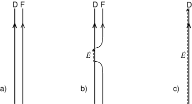
Figure 11: a) Parallel D-string and F-string. b) The F-string breaks, its ends attaching to the D-string. c) Final state: D-string with flux.

The F-string breaks, its endpoints attached to the D-string. The endpoints can then move off to infinity, leaving only the D-string behind. Of course, the D-string must now carry the charge of the F-string as well. This comes about because the F-string endpoints are charged under the D-string gauge field, so a flux runs between them; this flux remains at the end. Varying the NS-NS $B_{\mu\nu}$ field in the D-brane action (38), one sees that it has a source proportional to the invariant flux $F_{ab}+B_{ab}/2\pi\alpha^{\prime}$. Thus the final D-string carries both the NS-NS and R-R two-form charges. The flux is of order $g$, its energy density is of order $g$, and so the final tension is $(g^{-1}+O(g))/2\pi\alpha^{\prime}$. This is below the tension of the separated strings and of the same form as the BPS bound (108) for a $(1,1)$ string. A more detailed calculation shows that the final tension saturates the bound,[42] so the state is supersymmetric. In effect, the F-string dissolves in the D-string, leaving flux behind.

To calculate the number of BPS states we should put the strings in a box of length $L$ to make the spectrum discrete. For the $(1,0)$ F-string, the usual quantization of the ground state gives eight bosonic and eight fermionic states moving in each direction for $16^{2}=256$ in all. This is the ultrashort representation of supersymmetry: half the 32 generators annihilate the BPS state and the other half generate $2^{8}=256$ states. The same is true of the $(0,1)$ D-string and the $(1,1)$ bound state just found, as will be clear from the discussion of the D-string in the next lecture.

Incidentally, the $(1,0)$ F-string leaves unbroken half the supersymmetry and the $(0,1)$ D-string leaves unbroken a different half of the supersymmetry. The $(1,1)$ bound state leaves unbroken not the intersection of the two (which is empty), but yet a different half. The unbroken symmetries are linear combinations of the unbroken and broken supersymmetries of the D-string.

All the above extends immediately to $q$ F-strings and one D-string, forming a supersymmetric $(q,1)$ bound state. The more general case of $q_{1}$ F-strings and $q_{2}$ D-strings is more complicated. The gauge dynamics are now non-Abelian, the interactions are strong in the infrared, and no explicit solution is known. When $q_{1}$ and $q_{2}$ have a common factor, the BPS bound makes any bound state only neutrally stable against falling apart into subsystems. To avoid this complication let $q_{1}$ and $q_{2}$ be relatively prime, so any supersymmetric state is discretely below the continuum of separated states. This allows the Hamiltonian to be deformed to a simpler supersymmetric Hamiltonian whose supersymmetric states can be determined explicitly, and again there is one ultrashort representation, $256$ states. The details, which are a bit intricate, are left to the original reference.[22]

4.5 $0$-$p$ Bound States

Bound states of $p$-branes and $p^{\prime}$-branes have many applications. Here we focus on $p^{\prime}=0$, which can in general be reached by a $T$-duality.

0-0 bound states:

The BPS bound for the quantum numbers of $n$ 0-branes is $n\tau_{0}$, so any bound state will be at the edge of the continuum. To make the bound state counting well defined, compactify one direction and give the system momentum $m/R$ with $m$ and $n$ relatively prime.[57] The bound state now lies discretely below the continuum, because the momentum cannot be shared evenly among unbound subsystems.

This bound state problem is $T$-dual to the one just considered. Taking the $T$-dual, the $n$ 0-branes become D 1-branes, while the momentum becomes winding number, corresponding to $m$ F-strings. There is therefore one ultrashort multiplet of supersymmetric states when $m$ and $n$ are relatively prime.[57] This bound state should still be present back in infinite volume, since one can take $R$ to be large compared to the size of the bound state.

0-2 bound states: 

Now the BPS bound (110) puts any bound state discretely below the continuum. One can see a hint of a bound state forming by noticing that for a coincident 0-brane and 2-brane the NS 0-2 string has a negative zero-point energy (98) and so a tachyon (which survives the GSO projection), indicating instability towards something. In fact the bound state (one short representation) is easily described: the 0-brane dissolves in the 2-brane, leaving flux. The brane R-R action (89) contains the coupling $C_{(1)}F$, so with the flux the 2-brane also carries the 0-brane charge.[56] There is also one short multiplet for $n$ 0-branes. This same bound state is always present when $\nu=2$.

0-4 bound states:

The BPS bound (109) makes any bound state marginally stable, so the problem is made well-defined as in the 0-0 case by compactifying and adding momentum.[58] The interactions in the action (103) are relevant in the infrared so this is again a hard problem, but as before it can be deformed into a solvable supersymmetric system. Again there is one multiplet of bound states.[58] Now, though, the bound state is invariant only under $\frac{1}{4}$ of the original supersymmetry, the intersection of the supersymmetries of the 0-brane and of the 4-brane. The bound states then lie in a short (but not ultrashort) multiplet of $2^{12}$ states.

For $2$ 0-branes and one 4-brane, one gets the correct count as follows.[59] Think of the case that the volume of the 4-brane is large. The $16$ supersymmetries broken by the 4-brane generate $256$ states that are delocalized on the 4-brane. The 8 supersymmetries unbroken by the 4-brane and broken by the 0-brane generate $16$ states (half bosonic and half fermionic), localized on the 0-brane. The total number is the product $2^{12}$. Now count the number of ways two 0-branes can be put into their $16$ states on the 4-brane: there are $8$ states with both 0-branes in the same (bosonic) state and ${\textstyle{1\over 2}}16\cdot 15$ states with the D-branes in different states, for a total of $8\cdot 16$ states. But in addition, the two-branes can bind, and there are again $16$ states where the bound state binds to the 4-brane. Indirect arguments for the existence of these bound states have been given,[59] and presumably it can be demonstrated directly by the method used for 0-0 bound states in free space. The total, tensoring again with the 4-brane ground states, is $9\cdot 16\cdot 256$.

For $n$ 0-branes and one 4-brane, the degeneracy $D_{n}$ is given by the generating functional [59]

$$\sum_{n=0}^{\infty}q^{n}D_{n}\ =\ 256\ \prod_{k=1}^{\infty}\left(\frac{1+q^{k}}{1-q^{k}}\right)^{8}\ ,$$ (112)

where the term $k$ in the product comes from bound states of $k$ 0-branes then bound to the 4-brane.

0-6 bound states:

The relevant bound is (110) and again any bound state would be below the continuum. The NS zero-point energy for 0-6 strings is positive, so there is no sign of decay. One can give 0-brane charge to the 6-brane by turning on flux, but there is no way to do this and saturate the BPS bound. So it appears that there are no supersymmetric bound states. Incidentally, and unlike the 0-2 case, the 0-6 interaction is repulsive, both at short distance and [60] at long.

0-8 bound states:

I am confused by this case. There are two recent papers with some relevant observations.[61]

5 Lecture 5: Applications

5.1 String Duality

Now we can use D-branes to understand the strong-coupling limits of the theories in which they exist.

Type IIB:

Consider the D 1-brane of the IIB theory. The gauge field has no local dynamics, so the only bosonic excitations are the transverse fluctuations. The GSO projection on the open string Ramond ground state correlates the $SO(8)$ chirality with the right/left motion, so the right-moving spinors on the D-string are in the $\bf 8_{s}$ of $SO(8)$, and the left-moving spinors in the $\bf 8_{c}$. These are the same as the fluctuations of a fundamental IIB string.[22] There, the supersymmetries $Q_{\alpha}$ and $\tilde{Q}_{\alpha}$ have the same chirality. Half of each spinor annihilates the F-string and the other half generates fluctuations. Since the supersymmetries have the same $SO(9,1)$ chirality, the $SO(8)$ chirality is correlated with the direction of motion.

Up until now we have used the string metric, but for discussing string duality it is useful to switch to the Einstein metric, $g_{\mu\nu}^{\rm(E)}=g^{-1/2}g_{\mu\nu}^{\rm(s)}$. The Einstein metric, for which the gravitational action has no dependence on the dilaton, is an invariant under duality. The tensions are then

F-string: $$g^{1/2}/2\pi\alpha^{\prime}$$

D-string: $$g^{-1/2}/2\pi\alpha^{\prime}\ .$$ (113)

These are exact because of the BPS property.

At weak coupling the D-string is heavy and the F-string tension is the lightest scale in the theory. At strong coupling, however, the D-string is the lightest object in the theory, and it is natural to believe that the theory can be reinterpreted as a theory of weakly coupled D-strings, with $g^{\prime}=g^{-1}$. One cannot prove this without a nonperturbative definition of the theory, but quantizing the light D-string implies a large number of the states that would be found in the dual theory, and (Occam’s razor) self-duality of the IIB theory seems by far the simplest interpretation—given that physics below the Planck energy is described by some specific string theory, it seems likely that there is a unique extension to higher energies. This agrees with the duality deduced from the low energy action and other considerations.[36]${}^{\!-\,}$[38] In particular, the NS-NS and R-R two-form potentials, to which the D- and F-strings respectively couple, are interchanged by this duality.

The full duality group of the $D=10$ Type IIB theory is expected to be $SL(2,Z)$.[36]${}^{\!-\,}$[38] This relates the fundamental string not only to the R-R string but to a whole set of strings with the quantum numbers of $q_{1}$ F-strings and $q_{2}$ D-strings for $q_{1}$ and $q_{2}$ relatively prime.[55] The bound states found in section 4.4 are just what is required for $SL(2,Z)$ duality.[22] As the coupling and the R-R scalar are varied, each of these strings becomes light at the appropriate point in moduli space.

Type I:

For the D-strings of the Type I theory there are two modifications.[64] The first is the projection onto oriented states. The $U(1)$ gauge field, with vertex operator $\partial_{t}X^{\mu}$, is removed. The collective coordinates, with vertex operators $\partial_{n}X^{\mu}$, remain in the spectrum because the normal derivative is even under $\Omega$. That is, in terms of its action on the $X$ oscillators $\Omega$ has an additional $-1$ for the $m=2,\ldots,9$ directions, as compared to the action on the usual NN strings. By superconformal symmetry this must extend to the fermions, so that on the ground states $\Omega$ is no longer the identity but acts as $R=e^{i\pi(S_{1}+S_{2}+S_{3}+S_{4})}$. This removes the left-moving $\bf 8_{c}$ and leaves the right-moving $\bf 8_{s}$ (or vice versa: we have made an arbitrary choice in defining $R$).

The second modification is the inclusion of 1-9 strings, strings with one end on the 1-brane and one on a 9-brane, the latter corresponding to the usual $SO(32)$ Chan-Paton factor. This is the case $\nu=8$ from section 4.2.

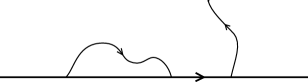
Figure 12: D-string in Type I theory with attached 1-1 and 1-9 strings.

The $\Omega$ projection determines the 9-1 state in terms of the 1-9, but otherwise makes no constraint. The zero point energy (98) is strictly positive so there are no massless states in the NS sector. The R ground states are, as always, massless. There are two ground states, from the periodic $\psi^{0,1}$ oscillators,

$$|\pm;i\rangle=(\psi^{0}_{0}\pm\psi^{1}_{0})|i\rangle,$$ (114)

where $i$ is the Chan-Paton index for the 9-brane end. One of the two states $|\pm;i\rangle$ is removed by the GSO projection, and the $G_{0}$ physical state condition on the remaining state implies that these massless fermions are chiral on the one-brane. Spacetime supersymmetry can only be satisfied if they move oppositely to the 1-1 fermions; at the world-sheet level this would have to follow from a careful analysis of the OPE of the gravitino. The 1-9 strings, having one 9-brane Chan-Paton index, are vectors of $SO(32)$.

Thus the world-sheet theory of the Type I one-brane is precisely that of the $SO(32)$ heterotic string, with the spacetime supersymmetry realized in Green-Schwarz form and the current algebra in fermionic form.[64] As in the IIB theory we can now argue that this $SO(32)$ heterotic string sets the lightest scale in the theory when $g$ becomes large, and so the natural assumption is that the strongly coupled behavior is governed by the weakly coupled heterotic string. This is in agreement with the conclusion from various other arguments.[38]${}^{\!,\,}$[65]

The fermionic $SO(32)$ current algebra requires a GSO projection. It is interesting to see how this arises in the D-string. Consider a closed D-string. The $\Omega$ projection removed the $U(1)$ gauge field, but is consistent with a discrete gauge symmetry, a holonomy $\pm 1$ around the D-brane. This discrete gauge symmetry is the GSO projection, and evidently the rules of D-branes require us to sum over all consistent possibilities in this way. We can now see how D-strings account for the spinor representation of $SO(32)$ in the Type I theory. In the R sector of the discrete D-brane gauge theory, the 1-9 strings are periodic. The zero modes of the fields $\Psi^{i}$, representing the massless 1-9 strings, satisfy the Clifford algebra

$$\{\Psi^{i}_{0},\Psi^{j}_{0}\}=\delta^{ij},\qquad i,j=1,\cdots,32.$$ (115)

The quantization now proceeds just as for the fundamental heterotic string, giving spinors ${\bf 2^{31}}+\overline{\bf 2^{31}}$, one of which is removed by the discrete gauge symmetry.

5.2 The Eleventh Dimension

One of the greatest surprises in string duality was the discovery of a new dimension, the eleventh. Let us see how we can find this dimension with the aid of D-branes.

Type IIA:

In the IIA theory, the 0-brane has a mass $\tau_{0}=\alpha^{\prime-1/2}g$ in the string metric. As $g\to\infty$, this mass is the lightest scale in the theory. In addition, we have seen in the previous lecture that $n$ 0-branes have a single supersymmetric bound state with mass $n\tau_{0}$. This evenly spaced tower of states is characteristic of the appearance of an additional dimension, where the momentum (Kaluza-Klein) states have masses $n/R$ and form a continuum is $R\to\infty$. The existence of these states and of the eleventh dimension was inferred even before the significance of D-branes was understood, because they are required by lower-dimensional $U$-dualities.[37]${}^{\!-\,}$[38]${}^{\!,\,}$

To relate the coupling to the size of the eleventh dimension we need to compare the respective actions,[38]

$$\frac{1}{2\kappa_{0}^{2}g^{2}}\int d^{10}x\,\sqrt{-g_{\rm s}}R_{\rm s}=\frac{2\pi R}{2\kappa_{11}^{2}}\int d^{10}x\,\sqrt{-g_{11}}R_{11}\ .$$ (116)

The string and M theory metrics are equal up to a rescaling,

$$g_{{\rm s}\mu\nu}=\zeta^{2}g_{{\rm 11}\mu\nu}$$ (117)

and so $\zeta^{8}=2\pi R\kappa_{0}^{2}g^{2}/\kappa_{11}^{2}$. The respective masses are related $nR^{-1}=m_{11}=\zeta m_{\rm s}=n\zeta\tau_{0}$ or $R=\alpha^{\prime 1/2}g/\zeta$. Combining these with the result (106) for $\kappa_{0}$, we obtain

$$\zeta=g^{1/3}\left[2^{7/9}\pi^{8/9}\alpha^{\prime}\kappa_{11}^{-2/9}\right]$$ (118)

and

$$R=g^{2/3}\left[2^{-7/9}\pi^{-8/9}\kappa_{11}^{2/9}\right]\ .$$ (119)

In order to emphasize the basic structure we hide in braces numerical factors and factors of $\kappa_{11}$ and $\alpha^{\prime}$. The former we hope are correct;  the latter are determined by dimensional analysis, with $\kappa_{11}$ having units of (M theory length^9/2) and $\alpha^{\prime}$ (string theory length²). We are free to set $\zeta=1$, using the same metric and units in M theory as in string theory. In this case

$$\kappa_{11}^{2}=g^{3}\left[2^{7}\pi^{8}\alpha^{\prime 9/2}\right]\ .$$ (120)

The reason for not always doing so is that when we have a series of dualities, as below, there will be different string metrics.

It is interesting to track the eleven-dimensional origin of the various branes of the IIA theory. The D 0-branes are, as we have just seen, Kaluza-Klein states. The F 1-branes, the IIA strings themselves, are wrapped membranes of M-theory.[66] The D 2-branes are membranes transverse to the eleventh dimension $X^{10}$. The D 4-branes are M-theory 5-branes wrapped on $X^{10}$, while the NS (symmetric) 5-branes are M-theory 5-branes transverse to $X^{10}$. The D 6-branes, being the magnetic duals of the 0-branes, are Kaluza-Klein monopoles. The D 8-branes are problematic, as there would seem to be no M-theory 8- or 9-branes from which they can descend. The point is that the D 8-branes, being sources of co-dimension one, cause the dilaton to diverge within a finite distance.[64] They must therefore be a finite distance from an orientifold plane, which is essentially a boundary of spacetime. As the coupling grows, the distance to the divergence and the boundary necessarily shrinks, so that they disappear into it in the strong coupling limit: they become part of the gauge dynamics of the nine-dimensional boundary of M-theory,[67] to be discussed in more detail below.

One can see further indication of the eleventh dimension in the dynamics of the D 2-brane. In $2+1$ dimensions, the vector field on the brane is dual to a scalar, through Hodge duality of the field strength, $*F_{2}=d\phi$. This scalar is the eleventh embedding dimension.[68]${}^{\!,\,}$[56] Carrying out the duality in detail, the D 2-brane action is found to have a hidden eleven-dimensional Lorentz invariance!

$E_{8}\times E_{8}$ Heterotic String:

We have deduced the duals of four of the five ten-dimensional string theories. Let us study the final one, the $E_{8}\times E_{8}$ heterotic string, by using its $T$-duality to the $SO(32)$ string.[69] Compactify on a large radius $R$ and turn on a Wilson line which breaks $E_{8}\times E_{8}$ to $SO(16)\times SO(16)$. This is $T$-dual to the $SO(32)$ heterotic string, again with a Wilson line breaking the group to $SO(16)\times SO(16)$. The couplings and radii are related

$$R^{\prime} = R^{-1}\left[\alpha^{\prime}\right],$$

$$g^{\prime} = gR^{-1}\left[{\alpha^{\prime}}^{1/2}\right]\ .$$ (121)

Now use Type I - heterotic duality to write this as a Type I theory with [38]

$$R_{\rm I} = g^{\prime-1/2}R^{\prime}\ =\ g^{-1/2}R^{-1/2}\left[\alpha^{\prime 3/4}\right],$$

$$g_{\rm I} = g^{\prime-1}\ =\ g^{-1}R\left[{\alpha^{\prime}}^{-1/2}\right]\ .$$ (122)

The radius is very small, so it is useful to make another $T$-duality, to the ‘Type I^′’ theory. The compact dimension is then a segment of length $\pi R_{\rm I^{\prime}}$ with eight D 8-branes at each end, and

$$R_{\rm I^{\prime}} = R_{\rm I}^{-1}\left[\alpha^{\prime}\right]\ =\ g^{1/2}R^{1/2}\left[\alpha^{\prime 1/4}\right],$$

$$g_{\rm I^{\prime}} = g_{\rm I}R_{\rm I}^{-1}\left[2^{-1/2}{\alpha^{\prime}}^{1/2}\right]\ =\ g^{-1/2}R^{3/2}\left[2^{-1/2}\alpha^{\prime-3/4}\right]\ .$$ (123)

Now take $R\to\infty$ to recover the original ten-dimensional theory (in particular the Wilson line is irrelevant and the original $E_{8}\times E_{8}$ restored). Both the radius and the coupling of the Type I^′ theory become large. The physics between the ends of the segment is given locally by the IIA string, and so the strongly coupled limit is eleven-dimensional. Taking into account the transformations (117), (119), the radii of the two compact dimensions in M-theory units are

$$R_{9} = \zeta_{\rm I^{\prime}}^{-1}R_{\rm I^{\prime}}\ =\ g^{2/3}\left[2^{-11/18}\pi^{-8/9}\kappa_{11}^{2/9}\right]$$ (124)

$$R_{10} = g_{\rm I^{\prime}}^{2/3}\left[2^{-7/9}\pi^{-8/9}\kappa_{11}^{2/9}\right]\ =\ g^{-1/3}R\left[2^{-10/9}\pi^{-8/9}\alpha^{\prime-1/2}\kappa_{11}^{2/9}\right]\ .$$

As $R\to\infty$, $R_{10}\to\infty$ also, while $R_{9}$ remains fixed and (for $g$ large) large compared to the Planck scale. Thus, in the strongly coupled limit of the ten-dimensional $E_{8}\times E_{8}$ heterotic string an eleventh dimension again appears, a segment of length $R_{9}$, with one $E_{8}$ factor on each endpoint.[67]

5.3 $U$-Duality

An interesting feature of string duality is the enlargement of the duality group under further toroidal compactification. Understanding the origin of these $U$-dualities, perhaps in some geometric way, might be a useful avenue to finding the underlying structure in string theory. Here I would like to describe one example, the Type II string on a five-torus. This is chosen because it is the setting for the simplest black hole state counting, and also because the necessary group theory is somewhat familiar from grand unification.

Let us first count the gauge fields. From the NS-NS sector there are 5 Kaluza-Klein gauge bosons and 5 gauge bosons from the antisymmetric tensor. There are 16 gauge bosons from the dimensional reduction of the various R-R forms. Finally, one can form a field strength from the Hodge dual $*H$ of the 3-form field strength of the NS-NS $B_{\mu\nu}$.

Let us see how $T$-duality acts on these. The $T$-duality is $SO(5,5;{\bf Z})$, generated by $T$-dualities on the various axes, linear redefinitions of the axes, and discrete shifts of the antisymmetric tensor. This mixes the first 10 NS-NS gauge fields among themselves, and the 16 R-R gauge fields among themselves, and leaves the final NS-NS field invariant. The $SO(5,5;{\bf Z})$ representations here correspond directly to the 10, 16, and 1 of $SO(10)$.

The low energy supergravity theory for this compactification has a continuous symmetry $E_{6(6)}$ which is a noncompact version of $E_{6}$.[70] This is one of those supergravity properties that was ignored for some time, because there is no sign of it in (perturbative) string theory. But now we know better: [36] a discrete subgroup $E_{6(6)}({\bf Z})$ is supposed to be a good symmetry of the full theory.

The gauge bosons are in the 27 of $E_{6(6)}({\bf Z})$, which is the same as the 27 of $E_{6(6)}$. The decomposition under $SO(10)\sim SO(5,5;{\bf Z})$ is familiar from grand unified model building,

$${\bf 27}\ \to\ {\bf 10}\ +\ {\bf 16}\ +\ {\bf 1}\ .$$ (125)

The excitations carrying the 10 charges are just the Kaluza-Klein and winding strings. The $U$-duality requires also states in the 16. These are just the various wrapped D-branes. Finally, the state carrying the 1 charge is an ordinary NS-NS soliton, a symmetric 5-brane.[71]

$U$-Duality and Bound States:

It is interesting to see how some of the bound state results from the previous lecture fit the predictions of $U$-duality. We will generate $U$-transformations as a combination of $T_{mn\cdots p}$, which is a $T$-duality in the indicated directions, and $S$, the IIB weak/strong transformation. The former switches between N and D boundary conditions and between momentum and winding number in the indicated directions. The latter interchanges the NS and R two-forms but leaves the R four-form invariant, and acts correspondingly on the solitons carrying these charges. We denote by ${\rm D}_{mn\cdots p}$ a D-brane extended in the indicated directions, and similarly for ${\rm F}_{m}$ a fundamental string and $p_{m}$ a momentum-carrying BPS state.

The first duality chain is

$$({\rm D}_{9},{\rm F}_{9})\ \stackrel{{\scriptstyle T_{78}}}{{\to}}\ ({\rm D}_{789},{\rm F}_{9})\ \stackrel{{\scriptstyle S}}{{\to}}\ ({\rm D}_{789},{\rm D}_{9})\ \stackrel{{\scriptstyle T_{9}}}{{\to}}\ ({\rm D}_{78},{\rm D}_{\emptyset})\ .$$ (126)

Thus the D-string–F-string bound state is $U$-dual to the 0-2 bound state.

The second chain is

$$({\rm D}_{6789},{\rm D}_{\emptyset})\ \stackrel{{\scriptstyle T_{6}}}{{\to}}\ ({\rm D}_{789},{\rm D}_{6})\ \stackrel{{\scriptstyle S}}{{\to}}\ ({\rm D}_{789},{\rm F}_{6})\ \stackrel{{\scriptstyle T_{6789}}}{{\to}}\ ({\rm D}_{6},p_{6})\ \stackrel{{\scriptstyle S}}{{\to}}\ ({\rm F}_{6},p_{6})$$ (127)

The bound states of $n$ 0-branes and $m$ 4-branes are thus $U$-dual to fundamental string states with momentum $n$ and winding number $m$. The bound state degeneracy (112) for $m=1$ precisely matches the fundamental string degeneracy.[72]${}^{\!,\,}$[58]${}^{\!-\,}$[73] For $m>1$ the same form (112) should hold but with $n\to mn$. This is believed to be the case, but the analysis (which requires the instanton picture described in the next section) does not seem to be complete.[73]

A related issue is the question of branes ending on other branes.[74] An F-string can of course end on a D-string, so from the first duality chain it follows that a D $p$-brane can end on a D $(p+2)$-brane. The key issue is whether the coupling between spacetime forms and world-brane fields allows the source to be conserved, as with the NS-NS two-form source in figure 11. Similar arguments can then be applied to the extended objects in M theory.[74]${}^{\!,\,}$[56]

5.4 D-Branes as Instantons

Consider now a 0-brane and $n$ coincident 4-branes. The potential terms in the action are

$$\frac{\chi_{i}^{\dagger}\chi_{i}}{(2\pi\alpha^{\prime})^{2}}\sum_{a=1}^{5}(X_{a}-Y_{a})^{2}+\frac{1}{4g_{0}^{2}}\sum_{I=1}^{3}(\chi_{i}^{\dagger}\tau^{I}\chi_{i})^{2}\ .$$ (128)

Here $a$ runs over the dimensions transverse to the 4-brane, and $X_{a}$ and $Y_{a}$ are respectively the 0-brane and 4-brane positions. This is the same as in the earlier action (103), except that we have taken the 4-branes to have infinite volume so that their $D$-term drops out, and the 0-4 field $\chi$ now carries a 4-brane index $i$ indicated explicitly (in addition to the $SU(2)_{R}$ index which is suppressed). The potential (128) is exact on grounds of $N=2$ supersymmetry. The first term is the $N=2$ coupling between the hypermultiplets $\chi$ and the vector multiplet scalars $X$, $Y$, while the second is the $U(1)$ $D$-term.

For $N>1$ there are two branches of moduli space,

$${\rm Coulomb\ branch\colon} X\neq Y,\quad\chi=0$$

$${\rm Higgs\ branch\colon} X=Y,\quad\chi\neq 0.$$ (129)

The Coulomb moduli space is just position space for the 0-brane. On the Higgs branch on the other hand, the 0-brane has gotten stuck on the 4-branes. In fact, it has dissolved into gauge fields, just as in the bound state discussions from the previous lecture. The R-R couplings include a term $C_{(1)}{\rm Tr}(F^{2})$, so that when there is an instanton on the 4-brane it carries the 0-brane charge. One can also check this from the dimension of moduli space. There are $4N$ real degrees of freedom in $\chi$. The vanishing of the $U(1)$ $D$-term imposes three constraints, and modding by the (broken) $U(1)$ removes another degree of freedom leaving $4N-4$. In addition there are the 4 moduli for the position of the 0-brane in the directions parallel to the 4-branes, for a total of $4N$ moduli. This is the correct number for an $SU(N)$ instanton when we do not mod out also the $SU(N)$ identifications. For $k$ instantons this becomes $4Nk$.

The connection between D-branes and instantons was found first in the case $(p,p^{\prime})=(9,5)$ by Witten.[53] This is $T$-dual to the above but does not have the Coulomb branch. That a $p$-brane instanton can shrink to zero size and move off as a $(p-4)$-brane was noted by Douglas.[43]

Note that this result has nothing to do with string duality, since the string coupling can be held fixed and small. Rather, it is a conformal field theory result. Starting from large instantons, it has always been a puzzle how to understand instanton amplitudes when the size of the instanton drops below the string scale. We now see, at least for instantons coupled to boundary (Chan-Paton) gauge fields, that there is a simple expansion around the zero-size limit.

5.5 D-Branes as Probes

In the preceding section we interpreted the 0-4 strings $\chi$ as moduli for the size and orientation of an instanton obtained as a blown-up D-brane. In a very interesting paper, Douglas has shown that one can see the resulting instanton by using another D-brane as a probe.[75] First take a $T$-dual so that the gauge fields live on 9-branes and the instanton is a 5-brane; then add a 1-brane as a probe. When the 1-brane is close to the 5-brane, closer than the string scale, the dynamics is dominated by the light open strings, especially the short 1-5 strings. Integrating out the light open strings to find the effective gauge field seen by the probe, one recovers Witten’s lagrangian version of the ADMH construction and so the instanton gauge field.[76]${}^{\!,\,}$[77] In particular, the variety of fields in that construction arise as the various $p$-$p^{\prime}$ strings of the D-brane system.

Thus it seems that one can sensibly discuss an instanton smaller than the string scale. This is in conflict with the idea that the string length is a minimum distance. Indeed, there were arguments to this effect made by Shenker,[78] and there have been recent studies of D-brane scattering suggesting that D-branes do indeed probe a shorter length scale.[24]${}^{\!,\,}$[79] This should be covered in detail in Steve’s lectures. There have been many other interesting recent applications of this idea, in particular by Seiberg, but I will not have time to pursue this.

I will sketch a different example of the D-brane as probe,[80] similar in nature to the instanton but simpler in its field content. This is the blowing up of a ${\bf Z}_{2}$ fixed point. It is known that twisted-sector moduli have the interpretation of smoothing out the orbifold geometry. With a D-brane probe this can be seen directly.

Consider the ${\bf R}^{6}\times({\bf R}^{4}/{\bf Z}_{2})$ orbifold formed by the reflection $R$, $X^{6,7,8,9}\to-X^{6,7,8,9}$, in the IIB theory. We are focusing on the neighborhood of a single fixed point. Add a D-string in this plane at $X^{2,\ldots,9}=0$. In order for the string to be able to move off the fixed plane it needs two Chan-Paton indices, for the string and its ${\bf Z}_{2}$ image. Since $R$ takes the D-string into its image, it acts on an open string state as

$$R|{\psi,ij}\rangle=\sigma^{1}_{ii^{\prime}}|{R\psi,i^{\prime}j^{\prime}}\rangle\sigma^{1}_{j^{\prime}j}\ .$$ (130)

That is, it acts on the oscillators in the usual way and also switches the Chan-Paton factors for the brane and its image. This is a simple example of the general formalism for orbifolds and orientifolds with D-branes.[54] In the NS sector, the massless $R$-invariant states are then

$$\partial_{t}X^{\mu}\sigma^{0,1},\qquad\mu=0,1$$

$$\partial_{n}X^{i}\sigma^{0,1},\qquad i=2,3,4,5$$

$$\partial_{n}X^{m}\sigma^{2,3},\qquad m=6,7,8,9.$$ (131)

These are respectively a gauge field, the position of the string within the six-plane, and the transverse position. Call the corresponding D-string fields $A^{\mu},x^{i},x^{m}$, all $2\times 2$ matrices. The bosonic action is the $d=10$ $U(2)$ Yang-Mills action, dimensionally reduced and $R$-projected (which breaks the gauge symmetry to $U(1)\times U(1))$. In particular, the potential is

$$U=2\sum_{i,m}{\rm Tr}([x^{i},x^{m}]^{2})+\sum_{m,n}{\rm Tr}([x^{m},x^{n}]^{2}).$$ (132)

The moduli space thus has two branches. On one, $x^{m}=0$ and $x^{i}=u^{i}\sigma^{0}+v^{i}\sigma^{1}$. This corresponds to two D-strings moving independently in the plane, with positions $u^{i}\pm v^{i}$. The gauge symmetry is unbroken, giving independent $U(1)$’s on each D-string. On the other branch, $x^{m}$ is nonzero and $x^{i}=u^{i}\sigma^{0}$. The $\sigma^{1}$ gauge invariance is broken and so by gauge choice $x^{m}=w^{m}\sigma^{3}$. This corresponds to the D-string moving off the fixed plane, the string and its image being at $(u^{i},\pm w^{m})$.

Now let us turn on twisted-sector moduli. Define complex $q^{m}$ by $x^{m}=\sigma^{3}{\rm Re}(q^{m})+\sigma^{2}{\rm Im}(q^{m})$, and define two doublets,

$$\Phi_{0}=\left(\begin{array}[]{c}q^{6}+iq^{7}\\ q^{8}+iq^{9}\end{array}\right),\qquad\Phi_{1}=\left(\begin{array}[]{c}\bar{q}^{6}+i\bar{q}^{7}\\ \bar{q}^{8}+i\bar{q}^{9}\end{array}\right).$$ (133)

These have charges $\pm 1$ respectively under the $\sigma^{1}$ $U(1)$. The three NSNS moduli can be written as a vector ${\bf D}$, and the potential is proportional to

$$(\Phi_{0}^{\dagger}\mbox{\boldmath$\tau$}\Phi_{0}-\Phi_{1}^{\dagger}\mbox{\boldmath$\tau$}\Phi_{1}+{\bf D})^{2},$$ (134)

where the Pauli matrices are now denoted $\tau^{I}$ to emphasize that they act in a different space. This reduces to the second term of the earlier potential (128) when ${\bf D}=0$. Its form is determined by supersymmetry.

For ${\bf D}\neq 0$ the orbifold point is blown up. The moduli space of the D-string is simply the set of possible locations, that is, the blown up ALE space. The $z^{m}$ contain eight scalar fields. Three are removed by the ${\bf D}$-flatness condition that the potential vanish, and a fourth is a gauge degree of freedom, leaving the expected four moduli. In terms of supermultiplets, the system has the equivalent of $d=6$ $N=1$ supersymmetry. The D-string has two hypermultiplets and two vector multiplets, which are Higgsed down to one hypermultiplet and one vector multiplet. The idea of Douglas [75] is that the metric on this moduli space, as seen in the kinetic term for the D-string fields, should be the smoothed orbifold metric. It is straightforward to verify this, and we omit the details.[80] The result is the Eguchi-Hanson metric,[81] which is the correct (hyper-Kähler) metric on the blown-up orbifold. This construction is known as the hyper-Kähler quotient.[82] This geometry seems to make sense even when its scale is far shorter than the string scale. This has recently been extended to other orbifolds.[83]

5.6 D-Branes as Black Holes

Before the significance of D-branes was recognized, the R-R charged objects required by string duality were believed to be black $p$-branes.[36]${}^{\!-\,}$[39] Such solutions exist for any tensor gauge charge,[35] with the source essentially hidden in the singularity. It is interesting to consider the relation between these two kinds of object.

Consider the action for the metric, an NS-NS field strength, and an R-R field strength, schematically

$$S=\int d^{D}x\,\left(e^{-2\phi}R-e^{-2\phi}H^{2}-G^{2}\right)\ .$$ (135)

For a black hole (or more generally $p$-brane) carrying NS-NS charge, the solution is determined by the balance between the first two terms. Since the dilaton appears in the same way in both terms, the classical solution is independent of the dilaton. That is, its size is independent of the string coupling and its mass scales as the action, $e^{-2\phi}=g^{-2}$. For a black $p$-brane carrying R-R charge, the solution is determined by a balance between the first and third terms. Its mass is then the mean, $e^{-\phi}=g^{-1}$, smaller at weak coupling than that of the NS-NS object. Similarly, one can see by a scaling argument that the size goes to zero with the string coupling. For couplings less than one, the classical solution is smaller than the string scale. At this point one’s prejudice from perturbative string theory is that geometry, or at least the low energy effective action we are using, makes no sense and the black solution is not relevant. Instead, as with the earlier example of instantons, for solitons smaller than the string scale D-branes provide the correct effective description.

One rather prosaic scenario for what all this means is that string theory really can be defined as some closed string field theory, and the D-branes are just solitons of this theory. The low energy action (135) is not valid for these solitons, but the full closed string action would correctly describe the D-branes. My own prejudice [84] is that string field theory is not likely to be a useful description beyond perturbation theory. String duality has reinforced this, in that each string theory appears to be an effective theory with a very specific range of validity.

It is interesting to consider now the case of $Q$ D-branes. Each boundary on the string world-sheet then brings in a factor of $gQ$, so the condition for validity of the D-brane approximation is now $gQ<1$. At the same time, one finds that the Schwarzchild radius in string units is also $gQ$, so the low energy geometric description should be valid for $gQ>1$.

Using a standard strategy in string duality we can continue in $g$ and the number of supersymmetric (BPS) states must be invariant. Strominger and Vafa applied this to a collection of D-branes chosen in such a way that the resulting black hole would have a nonzero area horizon, finding that the density of states in the D-brane system corresponded precisely to that given by the black hole entropy.[85] Because of the close analogy between black hole mechanics and thermodynamics, there have been many attempts to give a statistical mechanical interpretation to the black hole entropy, but this is the first time that it has been done in a controlled way.

This has of course led to a great surge of interest. Unfortunately this is beyond the scope of these lectures, but I should at least discuss in brief the implications for the black hole information paradox. At a superficial level there are none: the success of the state counting might be expected regardless. We have two descriptions with different ranges of validity, and while the D-brane system has an explicit quantum mechanical description, one could certainly imagine that at $gQ\sim 1$ the system makes a transition from being described to high accuracy by ordinary quantum mechanics to one with information loss.

Nevertheless, it is worth pushing things further and asking whether we can say more about black hole quantum mechanics from D-branes. Indeed, there are some successes that seem to go beyond what supersymmetry alone would require. These include  counting of states of some nonextremal black holes [87] and comparisons of the decay rates of black holes and D-branes [88] even at a fairly high level of detail. [89] Yet, even while there is some indication that black holes might be described by ordinary quantum mechanics, it is important to remember that there is a paradox here. Twenty years of attempts to show that information is preserved in black hole evaporation have only served to point up that if it is so it will imply a significant change in our way of thinking about spacetime. Enthusiasts of D-brane–black hole quantum mechanics should keep their eyes open for the important lesson.

5.7 Conclusion

The Theory of Everything—string theory, M-theory, whatever it should eventually be called—is now understood as in figure 13.

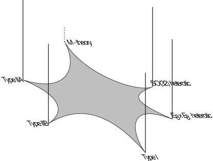
Figure 13: All string theories, and M-theory, as limits of one theory. Energy, or more generally distance from the BPS limit, increases vertically.

The various string theories are asymptotic expansions around the cusps. In addition, supergravity provides an effective description valid in the whole picture but only at low energy, and one can follow the BPS states from one limit to another.

This is far from a nonperturbative definition of the theory. I have no doubt that such a definition is possible, and that (as with the renormalization group in quantum field theory) it is a necessary step towards understanding the dynamics of the theory. Where do D-branes fit in? At a superficial level, they merely provide, in the Type I and Type II limits, a more precise description of the R-R solitons in the spectrum. Yet it may be that in fact they are closer than strings to being the fundamental degrees of freedom needed to define the whole picture. The fact that they probe shorter distance scales [79] and perhaps the unexpected successes of D-brane–black hole quantum mechanics described above suggest that this may be so. Thus, the D-brane Hamiltonian, or some structure abstracted from it, may have a much greater range of validity than the perturbative string theory in which it was first described.[90]

References

References

- [1] J. Dai, R. G. Leigh and J. Polchinski, Mod. Phys. Lett. A4 (1989) 2073.
- [2] J. Polchinski, Phys. Rev. Lett. 75 (1995) 4724.
- [3] J. Polchinski, S. Chaudhuri, and C. Johnson, Notes on D-Branes, preprint NSF-ITP-96-003, hep-th/9602052.
- [4] A. Chodos and C. B. Thorn, Nucl. Phys. B72 (1974) 509; W. Siegel, Nucl. Phys. B109 (1976) 244; S. M. Roy and V. Singh, Pramana 26 (1986) L85; Phys. Rev. D35 (1987) 1939.
- [5] J. A. Harvey and J. A. Minahan, Phys. Lett. B188 (1987) 44.
- [6] N. Ishibashi and T. Onogi, Nucl. Phys. B318 (1989) 239; G. Pradisi and A. Sagnotti, Phys. Lett. B216 (1989) 59; A. Sagnotti, Phys. Rept. 184 (1989) 167; P. Horava, Nucl. Phys. B327 (1989) 461.
- [7] P. Horava, Phys. Lett. B231 (1989) 251.
- [8] M. B. Green, Phys. Lett. B266 (1991) 325.
- [9] J. H. Schwarz, Nucl. Phys. B65 (1973), 131; E. F. Corrigan and D. B. Fairlie, Nucl. Phys. B91 (1975) 527; M. B. Green, Nucl. Phys. B103 (1976) 333; M. B. Green and J. A. Shapiro, Phys. Lett. 64B (1976) 454; A. Cohen, G. Moore, P. Nelson, and J. Polchinski, Nucl. Phys. B267, 143 (1986); B281, 127 (1987).
- [10] M. B. Green, Phys. Lett. B69 (1977) 89; B201 (1988) 42; B282 (1992) 380.
- [11] J. Polchinski, Phys. Rev. D50 (1994) 6041.
- [12] S. H. Shenker, in Cargese 1990, Proceedings: Random Surfaces and Quantum Gravity (1990) 191.
- [13] M. B. Green, Phys. Lett. B329 (1994) 435.
- [14] J. Paton and Chan Hong-Mo, Nucl. Phys. B10 (1969) 519.
- [15] J. H. Schwarz, in Florence 1982, Proceedings, Lattice Gauge Theory, Supersymmetry and Grand Unification, 233; Phys. Rept. 89 (1982) 223; N. Marcus and A. Sagnotti, Phys. Lett. 119B (1982) 97.
- [16] A. Sagnotti, Non-Perturbative Quantum Field Theory, eds. G. Mack et. al. (Pergamon Press, 1988) 521; V. Periwal, unpublished; J. Govaerts, Phys. Lett. B220 (1989) 77.
- [17] A. Strominger , S.-T. Yau, and E. Zaslow, Mirror Symmetry is -Duality, hep-th/9606040; H. Ooguri, Y. Oz, and Z. Yin, Nucl. Phys. B477 (1996) 407, hep-th/9606112.
- [18] K. Kikkawa and M. Yamanaka, Phys. Lett. B149 (1984) 357; N. Sakai and I. Senda, Prog. Theor. Phys. 75 (1986) 692.
- [19] V.P. Nair, A. Shapere, A. Strominger, and F. Wilczek, Nucl. Phys. B287 (1987) 402.
- [20] M. Dine, P. Huet, and N. Seiberg, Nucl. Phys. B322 (1989) 301.
- [21] P. Ginsparg and C. Vafa, Nucl. Phys. B289 (1987) 414; T. H. Buscher, Phys. Lett. B194B (1987) 59; B201 (1988) 466.
- [22] E. Witten, Nucl. Phys. B460 (1996) 335, hep-th/9510135.
- [23] R. G. Leigh, Mod. Phys. Lett. A4 (1989) 2767.
- [24] C. Bachas, Phys. Lett. B374 (1996) 37, hep-th/9511043.
- [25] E. Bergshoeff, M. de Roo, M. B. Green, G. Papadopoulos, and P.K. Townsend, Nucl. Phys. B470 (1996) 113, hep-th/9601150; E. Alvarez, J. L. F. Barbon, and J. Borlaf, -Duality for Open Strings, hep-th/9603089; E. Bergshoeff and M. De Roo, Phys. Lett. B380 (1996) 265, hep-th/9603123.
- [26] E. S. Fradkin and A. A. Tseytlin, Phys. Lett. B163 (1985) 123.
- [27] M. B. Green, C. M. Hull, and P. K. Townsend, Phys. Lett. B382 (1996) 65, hep-th/9604119.
- [28] S.P. de Alwis, A Note on Brane Tension and M Theory, hep-th/9607011.
- [29] C. Lovelace, Phys. Lett. B34 (1971) 500; L. Clavelli and J. Shapiro, Nucl. Phys. B57 (1973) 490; M. Ademollo, R. D’ Auria, F. Gliozzi, E. Napolitano, S. Sciuto, and P. di Vecchia, Nucl. Phys. B94 (1975) 221; C. G. Callan, C. Lovelace, C. R. Nappi, and S. A. Yost, Nucl. Phys. B293 (1987) 83.
- [30] J. Polchinski and Y. Cai, Nucl. Phys. B296 (1988) 91; C. G. Callan, C. Lovelace, C. R. Nappi and S.A. Yost, Nucl. Phys. B308 (1988) 221.
- [31] S. Coleman and E. Weinberg, Phys. Rev. D7 (1973) 1888; J. Polchinski, Comm. Math. Phys. 104 (1986) 37.
- [32] J. A. Shapiro and C. B. Thorn, Phys. Rev. D36 (1987) 432; J. Dai and J. Polchinski, Phys. Lett. B220 (1989) 387.
- [33] M. Douglas and B. Grinstein, Phys. Lett. B183 (1987) 552; (E) 187 (1987) 442; S. Weinberg, Phys. Lett. B187 (1987) 278; N. Marcus and A. Sagnotti, Phys. Lett. B188 (1987) 58.
- [34] D. Friedan, E. Martinec, and S. Shenker, Nucl. Phys. B271 (1986) 93.
- [35] G. T. Horowitz and A. Strominger, Nucl. Phys. B360 (1991) 197.
- [36] C. M. Hull and P.K. Townsend, Nucl. Phys. B438 (1995) 109.
- [37] P. K. Townsend, Phys. Lett. B350 (1995) 184, hep-th/9501068.
- [38] E. Witten, Nucl. Phys. B443 (1995) 85.
- [39] A. Strominger, Nucl. Phys. B451 (1995) 96.
- [40] L. J. Romans, Phys. Lett. B169 (1986) 374.
- [41] J. Polchinski and A. Strominger, New Vacua for Type II String Theory, hep-th/9510227.
- [42] M. Li, Nucl. Phys. B460 (1996) 351, hep-th/9510161.
- [43] M. R. Douglas, Branes within Branes, hep-th/9512077.
- [44] M. Bershadsky, C. Vafa, and V. Sadov, Nucl. Phys. B463 (1996) 420, hep-th/9511222.
- [45] M. B. Green, J. A. Harvey, and G. Moore, I-Brane Inflow and Anomalous Couplings on D-Branes, hep-th/9605033.
- [46] M. Bianchi, G. Pradisi, and A. Sagnotti, Nucl. Phys. B376 (1992) 365.
- [47] T. Banks and L. Susskind, Brane - Anti-Brane Forces, hep-th/9511194.
- [48] W. Fischler and L. Susskind, Phys. Lett. B171 (1986) 383; 173 (1986) 262.
- [49] M. B. Green and J. H. Schwarz, Phys. Lett. B149 (1984) 117; B151 (1985) 21.
- [50] S. Weinberg, The Quantum Theory of Fields. Vol. 1: Foundations, (Cambridge U. P., Cambridge UK, 1995).
- [51] R. I. Nepomechie, Phys. Rev. D31 (1985) 1921; C. Teitelboim, Phys. Lett. B167 (1986) 63, 69.
- [52] M. Berkooz, M. R. Douglas, and R. G. Leigh, Branes Intersecting at Angles, hep-th/9606139.
- [53] E. Witten, Nucl. Phys. B460 (1996) 541, hep-th/9511030.
- [54] E. G. Gimon and Joseph Polchinski, Phys. Rev. D54 (1996) 1667, hep-th/9601038.
- [55] J. H. Schwarz, Phys. Lett. B360 (1995) 13; (E) B364 (1995) 252.
- [56] P .K. Townsend, Phys. Lett. B373 (1996) 68, hep-th/9512062.
- [57] A. Sen, Phys. Rev. D54 (1996) 2964.
- [58] A. Sen, Phys. Rev. D53 (1996) 2874.
- [59] C. Vafa, Nucl. Phys. B463 (1996) 415, hep-th/9511088.
- [60] G. Horowitz, private communication.
- [61] G. Papadopoulos and P. K. Townsend, Kaluza-Klein on the Brane, hep-th/9609095; U. H. Danielsson and G. Ferretti, The Heterotic Life of the D-particle, hep-th/9610082.
- [62] C. M. Hull, Nucl. Phys. B468 (1996) 113, hep-th/9512181.
- [63] J. A. Harvey and A. Strominger, Nucl. Phys. B449 (1995) 535; A. Sen, Nucl. Phys. B450 (1995) 103.
- [64] J. Polchinski and E. Witten, Nucl. Phys. B460 (1996) 525, hep-th/9510169.
- [65] A. Dabholkar, Phys. Lett. B357 (1995) 307; C. M. Hull, Phys. Lett. B357 (1995) 545.
- [66] E. Bergshoeff, M. J. Duff, C. N. Pope, and E. Sezgin, Phys. Lett. B224 (1989) 71.
- [67] P. Horava and E. Witten, Nucl. Phys. B460 (1996) 506, hep-th/9510209.
-
[68]
M. J. Duff and J. X. Lu, Nucl. Phys. B390 (1993) 276, hep-th/9207060;
C. Schmidhuber, Nucl .Phys. B467 (1996) 146, hep-th/9601003;
S. P. de Alwis and K. Sato, Phys. Rev. D53 (1996) 7187, hep-th/9601167;
A. A. Tseytlin, Nucl. Phys. B469 (1996) 51, hep-th/9602064. -
[69]
K. S. Narain, Phys. Lett. 169B (1986) 41;
P. Ginsparg, Phys. Rev. D35 (1987) 648. - [70] B. Julia, in Supergravity and Superspace, ed. by S. W. Hawking and M. Rocek (Cambridge U. P., Cambridge UK, 1981).
- [71] C. G. Callan, J. A. Harvey, and A. Strominger, Nucl. Phys. B359 (1991) 611; B367 (1991) 60.
- [72] C. Vafa and E. Witten, Nucl. Phys. B431 (1994) 3, hep-th/9408074.
- [73] C. Vafa, Nucl. Phys. B463 (1996) 435, hep-th/9512078.
- [74] A. Strominger, Phys. Lett. B383 (1996) 44, hep-th/9512059.
-
[75]
M. Douglas, Gauge Fields and D-Branes, hep-th/9604198;
M. R. Douglas and G. Moore, D-Branes, Quivers, and ALE Instantons, hep-th/9603167. - [76] E. Witten, J. Geom. Phys. 15 (1995) 215, hep-th/9410052.
- [77] M. F. Atiyah, V. G. Drinfeld, N. J. Hitchin, and Y. I. Manin, Phys. Lett. A65 (1978) 185.
- [78] S. H. Shenker, Another Length Scale in String Theory? preprint RU-95-53, hep-th/9509132 and seminar at ITP, Jan. 1996.
-
[79]
D. Kabat and P. Pouliot, A Comment on Zero-Brane Quantum
Mechanics, hep-th/9603127;
U. H. Danielsson, G. Ferretti, and B. Sundborg, D-Particle Dynamics and Bound States, hep-th/9603081;
G. Lifschytz, Comparing D-branes to Black-branes, hep-th/9604156;
M. R. Douglas, D. Kabat, P. Pouliot and S. H. Shenker, D-branes and Short Distances in String Theory, hep-th/9608024. - [80] J. Polchinski, Tensors from Orientifolds, hep-th/9606165.
-
[81]
T. Eguchi and A. J. Hanson, Ann. Phys. 120 (1979) 82;
G. W. Gibbons and S. W. Hawking, Comm. Math. Phys. 66 (1979) 291. -
[82]
A. Hitchin, A. Karlhede, U. Lindstrom, and M. Roček,
Comm. Math. Phys. 108 (1987) 535;
P. Kronheimer, J. Diff. Geom. 28 (1989) 665; 29 (1989) 685. - [83] C. V. Johnson and R. C. Myers, Aspects of Type IIB Theory on ALE Spaces, hep-th/9610140.
- [84] J. Polchinski, “What is String Theory?,” Proceedings of the 1994 Les Houches Summer School, edited by F. David, P. Ginsparg and J. Zinn-Justin (Elsevier, Amsterdam, 1996) p. 287, hep-th/9411028.
- [85] A. Strominger and C. Vafa, Microscopic Origin of the Bekenstein-Hawking Entropy, hep-th/9601029.
- [86] F. Larsen and F. Wilczek, Phys. Lett. B375 (1996) 37.
-
[87]
C. G. Callan, Jr. and J. M. Maldacena, Nucl. Phys. B472
(1996) 591, hep-th/9602043;
G. T. Horowitz and A. Strominger, Phys. Rev. Lett. 77 (1996) 2368, hep-th/9602051;
G. T. Horowitz, J. M. Maldacena, and Andrew Strominger, Phys. Lett. B383 (1996) 151, hep-th/9603109;
J. M. Maldacena, Black Holes in String Theory, Ph. D. Thesis, hep-th/9607235. -
[88]
A. Dhar, G. Mandal and S. R. Wadia, Phys. Lett. B388 (1996) 51,
hep-th/9605234;
S. R. Das and Samir D. Mathur, Comparing Decay Rates for Black Holes and D-Branes, hep-th/9606185;
S. R. Das and S. D. Mathur, Interactions Involving D-Branes, hep-th/9607149. -
[89]
J. Maldacena and A. Strominger, Black Hole Grey Body Factors and D-Brane
Spectroscopy, hep-th/9609026;
C. G. Callan, Jr., S. S. Gubser, I. R. Klebanov, and A. A. Tseytlin, Absorption of Fixed Scalars and the D-Brane Approach to Black Holes, hep-th/9610172. - [90] T. Banks, W. Fischler, S. H. Shenker, and L. Susskind, M Theory as a Matrix Model: A Conjecture, hep-th/9610043.