Abstract

A new method is applied to solve the Baxter equation for three coupled, noncompact spins. Due to the equivalence with the system of three reggeized gluons, the intercept of the odderon trajectory is predicted for the first time, as the analytic function of the two relevant parameters.

TPJU-21/96
October 1996
hep-th/9610208

Calculation of the QCD prediction for the intercept of the odderon trajectory still remains a challenge for the Leading Logarithmic scheme of the reggeization of QCD [1, 2]. In the first approximation the problem naturally separates into sectors with fixed number $n$ of the reggeized gluons propagating in the $t$ channel. The lowest nontrivial case, $n=2$, was solved in the classical papers by Balitskii, Kuraev, Fadin and Lipatov [3] resulting in the simple expression for the intercept of the hard pomeron. The notable progress for arbitrary $n$ was achieved by Lipatov and Faddeev and Korchemsky [4, 5] who have established exact equivalence with the one dimensional chain of $n$ noncompact spins. Leading high energy behaviour of QCD amplitudes is given by the highest eigenvalue of the corresponding Heisenberg hamiltonian of $n$ spins with nearest neighbour interaction. Moreover, by identifying enough constants of motion they were able to prove that this system is soluble for arbitrary $n$. The success of this, rather mathematical, approach was confirmed by rederiving the Lipatov et al. result in the $n=2$ case [5, 6]. However, the adopted procedure requires an analytic continuation from the integer values of the relevant conformal weight $h$ (see later) because only for integer $h$ they were able to diagonalize the two spin hamiltonian. The $n=3$ case, which gives the lowest contribution to the odderon exchange, was also studied by Faddeev and Korchemsky, and Korchemsky [5, 6]. Again, the spectrum of the system for integer $h$ can be found for any finite $h=m$. However, the general expression for arbitrary $m$ is not known, and consequently the analytical continuation to $h=1/2$ is not available .

We have developed a new approach which a) works for arbitrary values of the conformal weight $h$, providing explicitly above continuation, and b) gives the analytic solution of the $n=3$ case for arbitrary $h$ and $q_{3}$. For $n=2$ our method reproduces again the $BFKL$ result clarifying the problem of boundary conditions for arbitrary $h$. This and the details of the $n=3$ calculation will be presented elsewhere [9]. In this letter we address directly the odderon case and discuss some phenomenological consequences.

The intercept of the odderon trajectory is given by

$$\alpha_{O}(0)=1+{\alpha_{s}N_{c}\over 4\pi}\left(\epsilon_{3}(h,q_{3})+\overline{\epsilon}_{3}(\overline{h},\overline{q}_{3})\right),$$ (1)

where $\epsilon_{3}$ and $\overline{\epsilon}_{3}$ are respectively the largest eigenvalues of the $n=3$ reggeon hamiltonian and its antiholomorphic counterpart [5, 6]. This system is equivalent to the one dimensional chain of three noncompact spins with nearest-neighbour interactions. Applying Bethe ansatz to the latter one obtains

$$\epsilon_{3}=i\left({\dot{Q}_{3}(-i)\over Q_{3}(-i)}-{\dot{Q}_{3}(i)\over Q_{3}(i)}\right)-6,$$ (2)

where $Q_{3}(\lambda)$ satisfies the following Baxter equation

$$(\lambda+i)^{3}Q_{3}(\lambda+i)+(\lambda-i)^{3}Q_{3}(\lambda-i)=(2\lambda^{3}+q_{2}\lambda+q_{3})Q_{3}(\lambda).$$ (3)

$q_{2}$ and $q_{3}$ are the eigenvalues of the two, commuting with the hamiltonian, operators which play important role in the proof of the solubility of the above system [4, 5]. The spectrum of $\hat{q}_{2}$ is known from the symmetry considerations

$$q_{2}=h(1-h),\;\;\;\;h={1\over 2}(1+m)-i\nu,\;\;m\in Z,\nu\in R.$$ (4)

The eigenvalues of $\hat{q}_{3}$ are known only for integer conformal weights $h$, whereas the value of $q_{3}$ for the ground state of the three reggeized gluons $(h=1/2)$ is not available. Analogous expressions hold for the antiholomorphic sector with $\overline{h}=(1-m)/2-i\nu$ [6].

Our goal is to determine $\epsilon_{3}(h,q_{3})$ for arbitrary $h$ and $q_{3}$. To this end we begin with the trick of Ref.[10] and seek the solution of the Baxter equation (3) in the form of the double contour representation

$$Q_{3}(\lambda)=\int_{C_{I}}Q_{I}(z)z^{-i\lambda-1}(1-z)^{i\lambda+1}dz+\int_{C_{II}}Q_{II}(z)z^{-i\lambda-1}(1-z)^{i\lambda+1}dz.$$ (5)

Provided the boundary contributions cancel, Eq.(3) is equivalent to the following ordinary differential equation for $Q_{I}(z)$ and $Q_{II}(z)$ $(\equiv Q(z))$

$$\left[\left(z(1-z){d\over dz}\right)^{3}-q_{2}z^{2}(1-z)^{2}{d\over dz}+iq_{3}z(1-z)\right]Q(z)=0.$$ (6)

This is a third order linear equation of the Fuchs class with the three regular singular points at $z=0,1$ and $\infty$, considered earlier in Refs. [6],[7],[8] We will prove that the complete boundary conditions on $Q_{I}(z)$ and $Q_{II}(z)$ are uniquely determined by the requirement of the cancellation of the boundary terms among the integrals (5). This is the distinctive feature of the $n=3$ case which allows for the successful application of our strategy.

We begin with the construction of the two fundamental sets of three, linearly independent solutions

$$\vec{u}(z)=(u_{1}(z),u_{2}(z),u_{3}(z)),$$ (7)

$$\vec{v}(z)=(v_{1}(z),v_{2}(z),v_{3}(z)),$$

around $z=0$ and $z=1$ respectively.

$$u_{1}(z) = \sum_{n=0}^{\infty}f_{n}z^{n},$$

$$u_{2}(z) = {1\over\pi i}\log{z}\;u_{1}(z)+{1\over\pi i}\sum_{n=0}^{\infty}r^{(1)}_{n}z^{n},$$ (8)

$$u_{3}(z) = {1\over\pi^{2}}\log^{2}{z}\;u_{1}(z)+{2\over\pi^{2}}\log{z}\;\sum_{n=0}^{\infty}r^{(1)}_{n}z^{n}+{1\over\pi^{2}}\sum_{n=0}^{\infty}r^{(2)}_{n}z^{n},$$

where the coefficients of the expansions are determined by the recursion relations easily obtained from Eq.(6).

$$f_{n+1} = (b_{n}f_{n}-c_{n-1}f_{n-1})/a_{n+1},\;\;f_{0}=1,\;f_{-1}=0,$$

$$a_{n} = n^{3},$$

$$b_{n} = iq_{3}+n(q_{2}+(2n+1)(n+1)),$$ (9)

$$c_{n} = n(q_{2}+(n+1)(n+2)),$$

and for the logarithmic solutions

$$r^{(1)}_{n+1} = (-p^{(1)}_{n}+b_{n}r^{(1)}_{n}-c_{n-1}r^{(1)}_{n-1})/a_{n+1},\;\;r^{(1)}_{0}=1,\;r^{(2)}_{-1}=0,$$

$$p^{(1)}_{n} = 3(n+1)^{2}f_{n+1}-(1+q_{2}+6n(n+1))f_{n}$$

$$+ (-1+q_{2}+3n^{2})f_{n-1},$$

$$r^{(2)}_{n+1} = (-p^{(2)}_{n}+b_{n}r^{(2)}_{n}-c_{n-1}r^{(2)}_{n-1})/a_{n+1},\;\;r^{(2)}_{0}=1,\;r^{(2)}_{-1}=0,$$

$$p^{(2)}_{n} = 6(n+1)f_{n+1}-6(2n+1)f_{n}+6nf_{n-1}$$ (11)

$$+ 6(n+1)^{2}r^{(1)}_{n+1}-2(1+q_{2}+6n(n+1))r^{(1)}_{n}$$ (12)

$$+ 2(2+q_{2}+3(n^{2}-1))r_{n-1}.$$ (13)

The series in Eq.(8) are convergent in the unit circle $K_{0}$ around $z=0$. Similarly one can construct the $\vec{v}(z)$ solutions in the unit circle $K_{1}$ around $z=1$. In fact, because of the symmetry of the Eq.(6) we take

$$\vec{v}(z;q_{2},q_{3})=\vec{u}(1-z;q_{2},-q_{3}),$$ (14)

Since any solution is the linear combination of the fundamental solutions, we have

$$Q_{I}(z)=au_{1}(z)+bu_{2}(z)+cu_{3}(z)\equiv A\cdot\vec{u}(z)=A\cdot\Omega\vec{v}(z),$$

$$Q_{II}(z)=du_{1}(z)+eu_{2}(z)+fu_{3}(z)\equiv B\cdot\vec{u}(z)=B\cdot\Omega\vec{v}(z),$$ (15)

with an obvious vector notation. The transition matrix $\Omega$ is defined by

$$\vec{u}(z)=\Omega\vec{v}(z),$$ (16)

and plays an important role in the following. It provides the analytic continuation of our solutions $Q(z)$ between $K_{0}$ and $K_{1}$. Transition matrix $\Omega$ can be easily determined from Eq.(16) once both bases, Eqs.(8,14), are known. For example, the i-th row, $\vec{\omega}_{i}^{T}$, of $\Omega$ can be obtained as

$$\vec{\omega}_{i}=(\Sigma^{T})^{-1}\vec{w}_{i},\;\;\;\Sigma_{kr}=v_{k}(z_{r}),\;\;(\vec{w_{i}})_{r}=u_{i}(z_{r}),\;\;\;i,k,r=1,2,3.$$ (17)

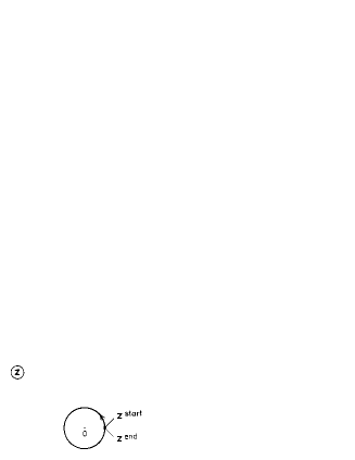
Figure 1: Closed contour used to define the monodromy matrix, Eq.(18). $z^{start}=z^{end}$, however they belong to the different sheets of the Riemann surface.

Where $z_{1},z_{2}$ and $z_{3}$ are arbitrary three points inside the intersection of $K_{0}$ and $K_{1}$. Next we introduce the monodromy matrix $M$ which describes the behaviour of the basis $\vec{u}$ in the vicinity of the branch point $z=0$ (see Fig.1)

$$\vec{u}(z_{end})=M\vec{u}(z_{start}),\;\;M=\left(\begin{array}[]{ccc}1&0&0\\ 2&1&0\\ -4&-4&1\end{array}\right).$$ (18)

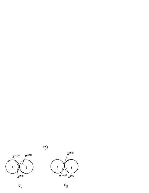
Figure 2: Integration contours used in Eq.(5). Start $z^{start}$, middle $z^{mid}$, and end $z^{end}$ points coincide but they lay on the different sheets of the Riemann surface of the integrands.

We are now ready to write the condition for the cancellation of the boundary contributions in Eq.(5). Let us choose the contours $C_{I}$ and $C_{II}$ as shown in Fig.2. Then, the boundary contributions cancel if

$$A^{T}M_{I}=P^{T},\;\;\;B^{T}M_{II}=-P^{T},\;\;\;P^{T}=(\alpha,\beta,\gamma),$$ (19)

where the combined monodromy matrices for the corresponding contours read

$$M_{I}=\Omega M\Omega^{-1}-M^{-1},\;\;M_{II}=\Omega M^{-1}\Omega^{-1}-M.$$ (20)

Hence the original freedom of six coefficients in Eqs.(15) was reduced to the three free parameters which we conveniently choose as $\alpha,\beta$ and $\gamma$. This was expected. However, in the n=3 case additional simplification occurs which, remarkably, allows to fix completely the remaining freedom.

The key point is the observation that the monodromy matrices (20) are singular, i.e. $det(M_{I})=det(M_{II})=0$. To see this it is enough to inspect the Riemann P symbol corresponding to Eq.(6).

$$P\left\{\begin{array}[]{ccc}0&1&\infty\\ 0&0&0\\ 0&0&1+h\\ 0&0&2-h\\ \end{array};z\right\}$$ (21)

It is readily seen that, contrary to the n=2 case, there exists a solution which is regular at $z=\infty$. Therefore the reduced monodromy matrices $M_{I}$ and $M_{II}$ must have the zero eigenvalue corresponding to this solution. As a consequence, Eqs.(19) do not have the unique solution for (a,…,f). Different choices of coefficients differ by the zero mode. This difference is inessential because the integrals of the solution, regular at infinity, vanish. We therefore proceed to isolate the zero mode explicitly, and then impose the condition of cancellation of boundary contributions. To this end we introduce the new basis $\vec{t}(z)$ such that $t_{3}(z)$ is the solution regular at $z=\infty$. Transformation matrix ${\cal T}$, $\vec{u}(z)={\cal T}\vec{t}(z)$, to the $\vec{t}(z)$ basis can be readily obtained by diagonalizing the commuting matrices $M^{A}=MM_{I}$ and $M^{B}=M_{II}M^{-1}$. In the new basis (marked by the subscript $t$) the cancellation condition reads

$$A_{t}^{\prime T}M_{t}^{A}=P_{t}^{T},\;\;\;B_{t}^{T}M_{t}^{B}=-P_{t}^{T}M_{t}^{-1},$$ (22)

where $M_{t}^{A}$ and $M_{t}^{B}$ are diagonal with one (third, say) zero eigenvalue, $A_{t}^{\prime T}\equiv(a_{t}^{\prime},b_{t}^{\prime},c_{t}^{\prime})=A_{t}^{T}M^{-1}_{t},$ and $M_{t}={\cal T}^{-1}M{\cal T}$ is the monodromy matrix in the new basis. Our final conclusions follow now trivially from Eq.(22). Coefficients $c_{t}^{\prime}$ and $f_{t}$ are arbitrary (and irrelevant), $\gamma_{t}=0$ and $a_{t}^{\prime},b_{t}^{\prime},d_{t},e_{t}$ are determined uniquely by $\alpha_{t}$ and $\beta_{t}$ provided the additional consistency condition

$$\alpha_{t}m_{13}+\beta_{t}m_{23}=0,$$ (23)

is satisfied, $m_{ik}$ being the matrix elements of $M_{t}^{-1}$. The last condition fixes completely the remaining freedom. Now the integral transforms $Q_{I}(z)$ and $Q_{II}(z)$ (hence also the solution of the Baxter equation $Q(\lambda))$ are determined uniquely up to an irrelevant normalization. This ends our proof.

Now the contour integrals and derivatives over $\lambda$ can be done analytically since $C_{I}$ and $C_{II}$ lay within the corresponding domains of convergence of all involved series . Integrating resulting expressions term by term we have obtained the final formula for $\epsilon_{3}(h,q_{3})$ in the form of absolutely convergent series for arbitrary values of the conformal weight $h$ and $q_{3}$. Resulting expression is rather lengthy and will not be quoted here, however it provides, for the first time, the energy of the three reggeon hamiltonian as the analytic function of the relevant parameters.

We will now discuss some special cases and phenomenological consequences of our result. First, for integer $h=m$ there exists a discrete set of quantized values of $q_{3}=q_{3}^{k}(m)$ for which the polynomial solution $u_{1}(z)$ exists. This quantization of $q_{3}$ is known and the eigenenergies $\epsilon_{3}(\overline{\epsilon_{3}})$ at these points can be calculated [6]. We quote the first few levels in Table 1.

h	$q_{3}$		$\epsilon_{3}$
4	$\pm 2\sqrt{3}$		$-7{1\over 2}$
5	$\pm 6\sqrt{3}$		$-8{5\over 6}$
6	$\pm 4\sqrt{3}$	$\pm 4\sqrt{30}$	$-9{1\over 4}$	$-10$

Table 1: Quantization of $q_{3}$ and first few levels of the holomorphic hamiltonian in the polynomial case.

Our formula reproduces these results exactly. The whole procedure can be followed in the polynomial case and it can be shown that the known spectrum emerges. Two particular cases are shown in Figs. 3a and 3b. In Fig.3a we plot $\epsilon_{3}(h,2\sqrt{3})$ around $h=4$, and in Fig.3b $\epsilon_{3}(6,q_{3})$ is shown in the region of $q_{3}$ which contains both positive eigenvalues $q^{(1,2)}_{3}(6)$ listed in Table I. All levels of $\epsilon_{3}$ (c.f. Table I) are reproduced. Second, our expression agrees with the asymptotic formula derived in Ref.[11]. In the limit $h,q_{3}\rightarrow\infty,\;\;q_{3}/h^{3}=const.$, Korchemsky has derived a simple expression

$$\epsilon_{3}(h,q_{3})=-2\log{2}-\sum_{k=0}^{3}\left[\psi(1+ihx_{k})+\psi(1-ihx_{k})-2\psi(1)\right],$$ (24)

where $x_{k},\;k=1,2,3$ are three roots of the polynomial $2h^{3}x^{3}+h^{2}(1-h)x+q_{3}$. Fig. 3c shows comparison of this asymptotic form with our exact formula for $q_{3}/h^{3}=1$. Agreement is very striking indeed and persists to $h$ as low as $h\sim 0.4$ . Interestingly, it turns out that the expression (24) contains many terms which are nonleading in the above limit. Retaining consistently the terms up to a given order in $1/h$, as was also done in Ref.[11], gives yet simpler result which however does not work so well. Also the analytic structure of $\epsilon_{3}(h,q_{3})$ is reasonably well reproduced by Eq.(24) while the rigorous expansion in $1/h$ fails here (see later).

Finally we discuss phenomenological consequences and relation with other works. Since the lowest state of the three reggeized gluons is expected to occur at $h=1/2$, we have mapped numerically the analytic structure of $\epsilon_{3}(1/2,q_{3})$ in the complex $q_{3}$ plane. Results are sketched in Fig.4. The holomorphic energy $\epsilon_{3}(1/2,q_{3})$ has a series of simple poles on the imaginary axis, and behaves regularly in the remaining part of the $q_{3}$ plane. In fact Re $\epsilon_{3}(1/2,q_{3})$ is negative almost in the whole $q_{3}$ plane except of the small regions in the vicinity of above poles. Interestingly, the approximate solution, Eq.(24), has the same singularity structure with similar location of poles. This suggests that there may exist a better, than $1/h$ expansion, approximation scheme in which Eq.(24) is the lowest order.

Because of Eq.(1) and the symmetry $(\overline{\epsilon}_{n}=\epsilon^{\star}_{n})$, the intercept of the odderon trajectory is smaller than $1$ for most values of $q_{3}$. In particular, $\alpha_{O}(0)<1$ for all real $q_{3}$. At the origin

$$\epsilon_{3}(1/2,0)=-.738\dots,$$ (25)

which indicates that the arguments used in Ref.[12] for the odderon intercept being exactly one, are incomplete. This discrepancy is caused by the degeneracy of the Baxter equations for two and three reggeized gluons when $q_{3}=0$. Continuity argument indicates that (25) is the true eigenvalue in the three reggeon sector.

A variational estimate of the lower bound for the odderon intercept $\alpha_{O}(0)>1+0.28g_{s}^{2}/\pi^{2}$ was derived in Ref.[13]. Together with present result it limits rather severely the allowed region of $q_{3}$ for the ground state of the system.

Due to the singularity structure seen above, the final prediction for $\alpha_{O}(0)$ requires however more detailed knowledge of the spectrum of $\hat{q}_{3}$. Some progress in this area has been reported in Refs.[14], [15].

Our approach may be generalized to higher $n$ [9]. Such a programme would provide the leading intercept of the $n$ reggeized gluons as the analytic function of the $n-1$ parameters $q_{2},\dots,q_{n}$.

We thank L. Lipatov and G. Korchemsky for interesting discussions. This work is supported by the Polish Committee for Scientific Research under grants no. PB 2P03B19609 and PB 2P03B08308.

Figures

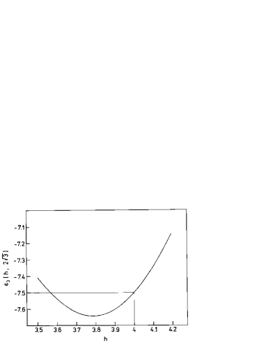
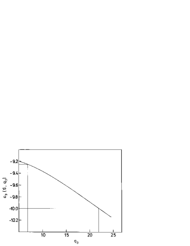
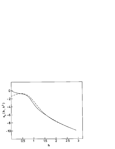
a
                                                     b
                                                     c

Figure 3: Holomorphic energy $\epsilon_{3}$ as the function of two continuous parameters. (a) at fixed $q_{3}=2\sqrt{3}$, (b) at fixed $h=6$ and (c) comparison with the asymptotic formula (dashed line), Eq.(24), described in text.

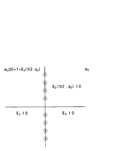
$\nwarrow$
                                $\swarrow$
                                                       $\bigcirc$

Figure 4: Schematic map of the analyticity structure of $\epsilon_{3}(1/2,q_{3})$ in the complex $q_{3}$ plane. $E_{3}$ is positive only in the vicinity of the poles.

References

- [1] H. T. Nieh and Y. -P. Yao, Phys. Rev. Lett., 32 (1974) 1074; Phys. Rev. D13 (1976) 1082. B. McCoy and T.T.Wu, Phys. Rev. D12 (1975) 3257.
- [2] J. Kwieciński and M. Praszałowicz, Phys. Lett. B94 (1980) 413; J. Bartels, Nucl. Phys., B175 (1980) 365; H. Cheng, J. Dickinson, C. Y. Lo and K. Olaussen, Phys. Rev. D23 (1981) 534;
- [3] E. A. Kuraev, L. N. Lipatov and V. S. Fadin, Phys. Lett. B60 (1975) 50; Sov. Phys. JETP 44 (1976) 443; ibid 45 (1977) 199; Ya. Ya. Balitskii and L. N. Lipatov, Sov. J. Nucl. Phys. 28 (1978) 822.
- [4] L. N. Lipatov, Padova preprint DFPD/93/TH/70 unpublished.
- [5] L. D. Faddeev and G. P. Korchemsky, Phys. Lett. B342 (1994) 311.
- [6] G. P. Korchemsky, Nucl. Phys. B443 (1995) 255.
- [7] Z. Maassarani and S. Wallon, J. Phys. A28 (1995) 6423.
- [8] R. A. Janik and J. Wosiek, Nucl. Phys., B(Proc.Suppl.)47 (1996) 771.
- [9] R. A. Janik and J. Wosiek, to be published; also in Proceedings of the ICHEP96 Conference, Warsaw, July 1996.
- [10] R. A. Janik, Acta Phys. Polon. B27 (1996) 1819 .
- [11] G. P. Korchemsky, Nucl. Phys. B462 (1996) 333.
- [12] N. Armesto and M. A. Braun, Univ. of Santiago de Compostella preprint, US-FT/7-96, hep-ph/9603218.
- [13] P. Gauron, L. N. Lipatov and B. Nicolescu, Zeit. Phys. C63 (1994) 253.
- [14] G. P. Korchemsky, Orsay preprint LPTHE-ORSAY-96-76, hep-th/9609123.
- [15] R. A. Janik, Phys. Lett. B371 (1996) 293.