Field Theory, Critical Phenomena and Interfaces
Gernot Münster
Institut für Theoretische Physik I
Westfälische Wilhelms-Universität
Wilhelm-Klemm-Str. 9
D-48149 Münster, Germany
Notes by H. Grießhammer and D. Lehmann
Institut für Theoretische Physik III
Friedrich-Alexander-Universität Erlangen-Nürnberg
Staudtstr. 7
D-91058 Erlangen, Germany

1 Field Theory

These lecture notes want to illustrate the close connection between statistical mechanics and field theory not only on the formal level, i.e. that many concepts of one area can easily be taken over to the other one, but also on the level of actual calculations. To this purpose, the last section will demonstrate that a special statistical system, the binary fluid system, can be described by field theory in its critical behaviour.

1.1 Canonical Formalism

Let us briefly review the setup of the canonical formalism of quantum field theory. For simplicity, we restrict ourselves to the case of a Hermitean scalar field $\phi(x)$ in Minkowski space.

There is a Hilbert space ${\cal H}$ of physical states $|\psi\,\rangle$, containing the vacuum $|0\,\rangle$ as the state of lowest energy. We assume that every state vector can be written as a linear combination of products of field operators acting on the vacuum $|0\,\rangle$. Furthermore, ${\cal H}$ carries a unitary representation $U(a,\Lambda)$ of the Poincaré group, where $a$ denotes a space-time translation and $\Lambda=(\Lambda^{\mu}\,_{\nu})$ a (homogeneous) Lorentz transformation. The vacuum is singled out by the fact that it is the only state vector which is invariant under $U(a,\Lambda)$. The generators $P_{\mu}$ of space-time translations,

$$U(a,{\rm 1\mskip-4.0mul})=\exp\left({\rm i}P_{\mu}a^{\mu}\right)\,,$$ (1)

have a spectrum which is confined to the closed forward light cone (“spectral condition”)

$$p^{2}=p_{\mu}\,p^{\mu}\geq 0\,;\qquad p^{0}\geq 0\,.$$ (2)

$P^{0}$ here denotes the Hamiltonian $H$. The scalar field $\phi(x)$ is a Hermitean, operator-valued distribution on ${\cal H}$, which transforms covariantly under Poincaré transformations:

$$U(a,\Lambda)\,\phi(x)\,U^{\dagger}(a,\Lambda)=\phi(\Lambda x+a)\,.$$ (3)

The theory is quantised by imposing canonical commutation relations between the fundamental field $\phi(x)$ and its canonical conjugate momentum $\pi(x)$ at equal times:

$$\begin{array}[]{rcl}{[}\,\phi(t,{\bf x}),\pi(t,{\bf y})\,{]}&=&{\rm i}\,\delta^{(3)}({\bf x}-{\bf y})\,,\\ {[}\,\phi(t,{\bf x}),\phi(t,{\bf y})\,{]}&=&{[}\,\pi(t,{\bf x}),\pi(t,{\bf y})\,{]}=0\,.\end{array}$$ (4)

Causality is guaranteed by requiring locality for the field, i.e. for space-like separations of the arguments the field operators must commute with each other:

$$[\,\phi(x),\phi(y)\,]=0\qquad\mbox{for}\qquad(x-y)^{2}\leq 0\,.$$ (5)

As the appearance of the $\delta$-distribution in (4) indicates, local field operators as $\phi(x)$ must be viewed as operator-valued distributions rather than functions and should be smeared out with appropriate test functions,

$$\phi(f)=\int\!\!{\rm d}^{4}x\,\,f(x)\,\phi(x)\,.$$ (6)

The smearing of $\phi(x)$ also in the time variable is necessary for interacting fields. Then, however, one can no longer postulate well-defined commutation relations at equal times [1]. An alternative to the Hilbert space formulation is to avoid operators and states and to introduce the functional integral as an independent way of quantising a theory. To make contact between both approaches, we introduce Green’s functions, which play a fundamental rôle in both formulations.

1.2 Green’s Functions

Vacuum expectation values of products of field operators

$$\begin{array}[]{rcl}{\cal W}(x_{1},\dots,x_{n})&:=&\langle\,0|\phi(x_{1})\dots\phi(x_{n})|0\,\rangle\vspace{2ex}\\ &=&\langle\,0|\phi(0,{\bf x_{1}}){\rm e}^{-{\rm i}(t_{1}-t_{2})H}\dots{\rm e}^{-{\rm i}(t_{n-1}-t_{n})H}\phi(0,{\bf x_{n}})|0\,\rangle\end{array}$$ (7)

are called $n$-point correlation functions or Wightman functions. A more prominent rôle in the Minkowski space formulation of field theory is played by time-ordered Green’s functions which are defined as the vacuum expectation values of time-ordered products of field operators,

$$\begin{array}[]{rcl}G(x_{1},\dots,x_{n})&:=&\langle\,0|{\cal T}\phi(t_{1},{\bf x_{1}})\dots\phi(t_{n},{\bf x_{n}})|0\,\rangle\vspace{2ex}\\ &=&\langle\,0|{\cal T}\biggl{\{}\phi(0,{\bf x_{1}}){\rm e}^{-{\rm i}(t_{1}-t_{2})H}\dots{\rm e}^{-{\rm i}(t_{n-1}-t_{n})H}\phi(0,{\bf x_{n}})\biggr{\}}|0\,\rangle\,;\end{array}$$ (8)

here ${\cal T}$ denotes the Dyson time ordering symbol,

$${\cal T}\{\phi(x_{1})\dots\phi(x_{n})\}:=\phi(x_{\pi(1)})\dots\phi(x_{\pi(n)})\qquad{\rm with}\qquad t_{\pi(1)}\geq t_{\pi(2)}\geq\dots\geq t_{\pi(n)}\,.$$ (9)

They can be directly related to S-matrix elements via the well-known Lehmann-Symanzik-Zimmermann (LSZ) reduction formulae. E.g., the S-matrix element between an out-state with momenta $q_{1},\dots,q_{l}$ and an in-state with momenta $p_{1},\dots,p_{n}$ is given by

$$\begin{array}[]{l}\langle\,p_{1},\dots,p_{n},{\rm in}|{\rm S}|q_{1},\dots,q_{l},{\rm out}\,\rangle=\\ \qquad=({\rm i}Z^{-1/2})^{n+l}{\displaystyle\int}\!{\rm d}^{4}y_{1}\dots{\rm d}^{4}x_{l}\,\,\exp\left({\rm i}\sum\limits_{k=1}^{n}p_{k}\cdot y_{k}-{\rm i}\sum\limits_{r=1}^{l}q_{r}\cdot x_{r}\right)\\ \qquad\times\left(\Box_{y_{1}}+m^{2}\right)\cdots\left(\Box_{x_{l}}+m^{2}\right)\,\,G(y_{1},\dots,x_{l})\,,\end{array}$$ (10)

where $Z$ is an appropriate normalisation factor. For more details on the LSZ formalism the reader is referred to a standard textbook on quantum field theory, e.g. Refs. [2], [3].

The most important fact about Green’s functions is that they contain all the information about the theory. So, given either all the Wightman or all the time-ordered correlation functions we may construct the Hilbert space and the unitary representation $U(a,\Lambda)$ out of them (this is the essence of the so-called reconstruction theorem, [4], [5]). Thus, we may use the Green’s functions to define the theory, thereby avoiding the operator formulation altogether.

1.3 Euclidean Time Formulation

Another important ingredient in our formulation of Euclidean field theory is the analytic continuation to imaginary times:

$$x^{0}\to-{\rm i}x^{4},\enspace x^{4}\in{\rm I\!R}\,.$$ (11)

This is convenient for several reasons. Generally speaking, it improves the analytic behaviour of the various relevant functions. In perturbation theory it simplifies the calculation of Feynman diagrams, e.g. because of the positivity of the energy denominators. Moreover, since in Euclidean space all distinct world-points are space-like separated, the Euclidean Green’s functions are automatically symmetric (for bosons) in all their space-time arguments, and we do not need any time-ordering. Thus, in Euclidean space we have to deal with only one kind of Green’s functions and both, the Wightman and the time-ordered Minkowski space Green’s functions, may be obtained from the Euclidean ones by appropriate analytic continuation. Last not least, the functional-integral formulation to be introduced in section (1.5) is much better defined in the Euclidean formulation due to the positivity of the Euclidean Green’s functions and may be interpreted as a stochastic process.

Consider the analytic continuation of the Wightman functions to complex time arguments $x^{0}_{i}\to x^{0}_{i}-{\rm i}x^{4}_{i}\,,\quad x_{i}^{0},x_{i}^{4}\in{\rm I\!R}\,$:

$$\begin{array}[]{l}{\cal W}(x^{0}_{1}-{\rm i}x^{4}_{1},{\bf x_{1}};\dots;x^{0}_{n}-{\rm i}x^{4}_{n},{\bf x_{n}})=\\[12.91663pt] \quad=\langle\,0|\phi(0,{\bf x_{1}}){\rm e}^{-{\rm i}(x^{0}_{1}-x^{0}_{2})H}{\rm e}^{-(x^{4}_{1}-x^{4}_{2})H}\phi(0,{\bf x_{2}})\dots\phi(0,{\bf x_{n}})|0\,\rangle\,.\end{array}$$ (12)

Due to the positivity of the Hamiltonian this is well-defined and analytic at least for

$$x^{4}_{1}>x^{4}_{2}>\dots>x^{4}_{n}\,,$$ (13)

since we have exponential suppression in this domain. We define the Euclidean Green’s functions, also called Schwinger functions, as the $x^{0}_{i}\to 0$ limit of the analytically continued Wightman functions:

$$\begin{array}[]{rcl}{\cal S}({\bf x_{1}},x^{4}_{1};\dots;{\bf x_{n}},x^{4}_{n})&:=&{\cal W}(-{\rm i}x^{4}_{1},{\bf x_{1}};\dots;-{\rm i}x^{4}_{n},{\bf x_{n}})=\\[12.91663pt] &=&\langle\,0|\phi(0,{\bf x_{1}}){\rm e}^{-(x^{4}_{1}-x^{4}_{2})H}\dots{\rm e}^{-(x^{4}_{n-1}-x^{4}_{n})H}\phi(0,{\bf x_{n}})|0\,\rangle\,.\end{array}$$ (14)

For the time being this is only legitimate if the condition (13) is fulfilled. It can, however, be shown [4] that the region of analyticity is much larger and the Schwinger functions are actually well-defined for all non-coinciding Euclidean world-points:

$$x_{i}\neq x_{j}\qquad\mbox{for}\qquad i\neq j\,.$$ (15)

Figure 1: The analyticity region of the two-point function $W(x)$ in the complex $x^{0}$-plane. The Wightman function $W$ is obtained by approaching the real line from below. The Schwinger function is defined on the imaginary $x^{0}$-axis. The time-ordered Green’s function $G$ is obtained from the Schwinger function by means of a Wick rotation, indicated by curved arrows.

Let us demonstrate this for the two-point function: The translational invariance of the vacuum implies that ${\cal W}$ depends only on the difference of its arguments

$${\cal W}(x_{1},x_{2})=W(x_{1}-x_{2})\,,$$ (16)

which can be seen explicitly from (12). As a function of complex $x^{0}$, $W$ is analytic in the lower half plane. For permuted arguments we have

$${\cal W}(x_{2},x_{1})=W_{\pi}(x_{1}-x_{2})=W(x_{2}-x_{1})\qquad\mbox{with}\qquad W_{\pi}(x):=W(-x)\,,$$ (17)

where $W_{\pi}$ is now analytic in the upper half plane according to (13). For space-like separations, $(x_{1}-x_{2})^{2}<0$, however, the Wightman function is symmetric due to locality:

$${\cal W}(x_{1},x_{2})={\cal W}(x_{2},x_{1})\,,$$ (18)

implying

$$W_{\pi}(x)=W(x)$$ (19)

in the non-discrete region

$$\quad-|{\bf x}|<x^{0}<|{\bf x}|$$ (20)

of the real axis. The well-known edge-of-the-wedge theorem then guarantees that $W$ and $W_{\pi}$ form a single, analytic function in the union of their domains, i.e. everywhere in the complex $x^{0}$ plane except along the cuts $|x^{0}|>|{\bf x}|$.

The Schwinger functions and their properties have been studied in an axiomatic setting by Osterwalder and Schrader [6]. For our purposes the most interesting properties are

1. Euclidean covariance:

   $${\cal S}(\Lambda x_{1}+a,\dots,\Lambda x_{n}+a)={\cal S}(x_{1},\dots,x_{n})\,,\qquad\Lambda\in\mbox{SO}(4)\,,$$ (21)

   where the Lorentz group of (3) is replaced by the group of Euclidean rotations.

2. Symmetry:

   $${\cal S}(x_{\sigma(1)},\dots,x_{\sigma(n)})={\cal S}(x_{1},\dots,x_{n})\,,$$ (22)

   where $\sigma$ is a permutation. This rests on the fact that distinct Euclidean points are always space-like relative to each other.

3. Reflection positivity: This property replaces the Hilbert space positivity and the spectral condition (2) of the Minkowskian formulation and is necessary to guarantee that the Euclidean correlation functions may be continued back to Minkowski space. Formally, it is defined as

   $$\begin{array}[]{l}\displaystyle\sum\limits_{i,j}\int\!{\rm d}^{4}x_{1}\dots{\rm d}^{4}x_{i}\,{\rm d}^{4}y_{1}\dots{\rm d}^{4}y_{j}\enspace f_{i}^{\ast}(x_{1},\dots,x_{i})\,f_{j}(y_{1},\dots,y_{j})\\ \qquad\times{\cal S}(\theta x_{1},\dots,\theta x_{i},y_{1},\dots,y_{j})\geq 0\,,\end{array}$$ (23)

   where $\theta$ is the Euclidean time reflection,

   $$\theta({\bf x},x^{4}):=({\bf x},-x^{4})\,,$$ (24)

   which, roughly speaking, replaces the Hermitean conjugation in Minkowski space.

A Euclidean quantum field theory may be defined by the set of all its Schwinger functions. From them the Wightman functions in Minkowski space can be reconstructed as boundary values:

$${\cal W}(x_{1},\dots,x_{n})=\lim\limits_{\begin{array}[]{c}\scriptstyle\varepsilon_{i}\to 0,\\ \scriptstyle\varepsilon_{i}-\varepsilon_{i+1}>0\end{array}}{\cal S}({\bf x_{1}},\varepsilon_{1}+{\rm i}x^{0}_{1};\dots;{\bf x_{n}},\varepsilon_{n}+{\rm i}x^{0}_{n})\,,$$ (25)

i.e. approaching the real $x^{0}$-axis from below in the case of the two-point function, see Fig. 1. The advantage of the Euclidean formulation, however, is that the Schwinger functions obey simpler properties and are easier to handle than Wightman functions or field operators. In particular their symmetry is the crucial property which opens the way to a representation in terms of functional integrals.

The time-ordered Green’s functions $G(x_{1},\dots,x_{n})$ may also be obtained from the Schwinger functions, namely by approaching the real $x^{0}$-axis through a counter-clockwise rotation of $\pi/2$ as indicated in Fig. 1,

$$G(x_{1},\dots,x_{n})=\lim\limits_{\alpha\to\pi/2}{\cal S}({\rm e}^{{\rm i}\alpha}x^{0}_{1},\dots,{\rm e}^{{\rm i}\alpha}x^{0}_{n})\,.$$ (26)

This rule, which obviously is simpler than the one for the Wightman functions, is called Wick rotation.

1.4 Example: Free Field

To illustrate the analytic continuation discussed above, let us consider the simplest case of a free massive Hermitean scalar field $\phi(x)$, decomposed in momentum space as [3]

$$\phi(x)=\int\!\frac{{\rm d}^{3}k}{(2\pi)^{3}2\omega_{k}}\,\,\left[a(k){\rm e}^{-{\rm i}kx}+a^{\dagger}(k){\rm e}^{{\rm i}kx}\right]\,,$$ (27)

with $k^{0}=\omega_{k}=\sqrt{{\bf k}^{2}+m^{2}}$. The annihilation and creation operators satisfy the commutation relations

$$[\,a(k),a^{\dagger}(k^{\prime})\,]=(2\pi)^{3}\,2\omega_{k}\,\delta^{3}({\bf k}-{\bf k}^{\prime})\,.$$ (28)

The two-point Wightman function then is given by

$$W(x)={\cal W}(x,0)=\langle\,0|\phi(x)\phi(0)|0\,\rangle=\Delta_{+}(x)={\displaystyle\int\!\!\frac{{\rm d}^{4}k}{(2\pi)^{4}}}\,\,\delta(k^{2}-m^{2})\,\theta(k^{0}){\rm e}^{-{\rm i}kx}\,.$$ (29)

The time-ordered two-point Green’s function, the Feynman propagator, reads

$${\rm i}\Delta_{\rm F}(x):=G(x,0)=\theta(x^{0})W(x)+\theta(-x^{0})W(-x)={\displaystyle\int\!\!\frac{{\rm d}^{4}k}{(2\pi)^{4}}\,\,\frac{{\rm e}^{-{\rm i}kx}}{k^{2}-m^{2}+{\rm i}\varepsilon}}\,.$$ (30)

Performing the analytic continuation of $W(x)$ yields

$${\cal S}(x,0)=\int\!{\displaystyle\frac{{\rm d}^{4}k}{(2\pi)^{4}}}\,\,{\displaystyle\frac{{\rm e}^{{\rm i}kx}}{k^{2}+m^{2}}}\quad=\,\frac{m}{(2\pi)^{2}|{\bf x}|}\ {\rm K}_{1}(m|{\bf x}|)\,.$$ (31)

$G(x,0)$ is obtained from ${\cal S}(x,0)$ by means of a Wick rotation of $x^{4}={\rm i}x^{0}$ in a counter-clockwise sense. In the integral we have to rotate at the same time $k^{4}={\rm i}k^{0}$ in a clockwise sense. The resulting integration path in the complex $k^{0}$-plane bypasses the poles at $\pm\sqrt{{\bf k}^{2}+m^{2}}$ in the way indicated by the $+{\rm i}\varepsilon$ prescription. It goes from $+\infty$ to $-\infty$, and an additional sign change has to be introduced to bring it in the form above. Note that the long distance behaviour of the Schwinger function is exponential and governed by the mass $m$:

$${\cal S}(x,0)\stackrel{{\scriptstyle|{\bf x}|\to\infty}}{{\longrightarrow}}\frac{m^{2}}{2(2\pi m|{\bf x}|)^{3/2}}\ \exp\left(-m|{\bf x}|\right)\,.$$ (32)

1.5 Functional Integral Formulation

The symmetry property of the Schwinger functions means that the Euclidean fields commute. In this respect they behave like classical fields. This allows us to interpret the $\phi(x)$’s as classical random variables instead of quantum mechanical operators. In this interpretation the Schwinger functions are the $n-$point correlation functions or moments of an appropriate probability measure ${\rm d}\mu[\phi]$:

$${\cal S}(x_{1},\dots,x_{n})=\langle\,\phi(x_{1})\dots\phi(x_{n})\,\rangle=\int\!{\rm d}\mu[\phi]\,\,\phi(x_{1})\dots\phi(x_{n})\,.$$ (33)

We may define a generating functional for the Schwinger functions as the Laplace transform of the probability measure,

$$\begin{array}[]{l}{\cal Z}[j]:=\displaystyle\biggl{\langle}\,\exp\left(\int\!{\rm d}^{4}x\,\phi(x)j(x)\right)\,\biggr{\rangle}\\[12.91663pt] \qquad\displaystyle=\sum\limits_{n=0}^{\infty}\,\frac{1}{n!}\int\!{\rm d}^{4}x_{1}\dots{\rm d}^{4}x_{n}\,j(x_{1})\dots j(x_{n})\,\langle\,\phi(x_{1})\dots\phi(x_{n})\,\rangle\,,\end{array}$$ (34)

from which the moments are obtained by functional differentiation with respect to the external sources $j(x)$:

$$\langle\,\phi(x_{1})\dots\phi(x_{n})\,\rangle=\frac{\delta^{n}{\cal Z}[j]}{\delta j(x_{1})\dots\delta j(x_{n})}\Bigg{|}_{j=0}\,.$$ (35)

Thus the generating functional ${\cal Z}[j]$ summarises all the information about the theory in a highly condensed form.

Formally, one may decompose ${\rm d}\mu[\phi]$ in a product of a “Lebesgue” measure ${\cal D}[\phi]$ on function space and a normalised weight factor

$${\rm d}\mu[\phi]=\frac{1}{{\cal Z}}\,{\cal D}[\phi]\,{\rm e}^{-S_{\rm E}[\phi]}\,,$$ (36)

where $S_{\rm E}[\phi]$ is the Euclidean action of the field $\phi$,

$$S_{\rm E}[\phi]=\int\!{\rm d}^{4}x\,\left\{\frac{1}{2}\,\partial_{\mu}\phi(x)\,\partial_{\mu}\phi(x)+{\displaystyle\frac{m^{2}}{2}}\phi^{2}(x)+V\left(\phi(x)\right)\right\}\,.$$ (37)

This yields the functional integral formulation of the Euclidean correlation function and the generating functional:

$${\cal Z}[j] = {\displaystyle\frac{1}{{\cal Z}}\,\int}\!{\cal D}[\phi]\,\,\exp\left(-S_{\rm E}[\phi]+\int\!{\rm d}^{4}x\,\phi(x)j(x)\right)\,,\vspace{2ex}$$ (38)

$$\langle\,\phi(x_{1})\dots\phi(x_{n})\,\rangle = {\displaystyle\frac{1}{{\cal Z}}}\,{\displaystyle\int}\!{\cal D}[\phi]\,\phi(x_{1})\dots\phi(x_{n})\,{\rm e}^{-S_{\rm E}[\phi]}\,,$$ (39)

where ${\cal Z}$ is introduced to normalise the generating functional to ${\cal Z}[0]=1$,

$${\cal Z}={\displaystyle\int}\!{\cal D}[\phi]\ {\rm e}^{-S_{\rm E}[\phi]}\,.$$ (40)

However, as it stands, (36) is a purely formal definition since a translational invariant Lebesgue measure like ${\cal D}[\phi]$ does not exist on the infinite-dimensional function space of the continuum field theory.

1.6 Lattice Regularisation

We can give a precise meaning to the functional integral expressions of the preceeding section, if we refer to a lattice regularisation of the Euclidean field theory. This means, we replace the Euclidean space-time continuum by a finite hyper-cubical lattice with lattice spacing $a$,

$$x_{\mu}=an_{\mu}\,,\qquad n_{\mu}\enspace\mbox{integer-valued}\,.$$ (41)

One may think of the lattice field $\phi(x)$ as the average of the continuum field over the volume of the elementary cells of the lattice. In momentum space, the lattice regularisation reflects itself in the restriction of the momenta to the first Brillouin zone,

$${\cal B}=\biggl{\{}p_{\mu}\Bigg{|}-{\displaystyle\frac{\pi}{a}}\leq p_{\mu}\leq{\displaystyle\frac{\pi}{a}}\biggr{\}}\,.$$ (42)

On a finite lattice the function space is finite-dimensional, and the measure ${\cal D}[\phi]$ can be defined as the multi-dimensional Lebesgue measure

$${\cal D}[\phi]:=\prod\limits_{x}{\rm d}\phi(x)\,,$$ (43)

where $x$ runs over all lattice points. Space-time integrals are replaced by sums and the differential operators $\partial_{\mu}$ are replaced on the lattice by nearest-neighbour forward differences,

$$\begin{array}[]{l}\displaystyle\int\!{\rm d}^{4}x\,\to\sum\limits_{x}\,a^{4}\,,\\ \partial_{\mu}\,\phi(x)\to\Delta_{\mu}\phi(x):={\displaystyle\frac{1}{a}}\,\biggl{(}\phi(x+a\hat{\mu})-\phi(x)\biggr{)}\,,\end{array}$$ (44)

where $\hat{\mu}$ is the unit vector in $\mu$-direction. This yields the lattice analogue of (37):

$$\begin{array}[]{rcl}S_{\rm E}[\phi]&=&\displaystyle\frac{1}{2}\sum\limits_{x}a^{4}\ \biggl{\{}\left(\Delta_{\mu}\phi(x)\right)\left(\Delta_{\mu}\phi(x)\right)+{\displaystyle\frac{m_{0}^{2}}{2}}\phi^{2}(x)+V(\phi(x))\biggr{\}}\\ &=&\displaystyle\sum\limits_{x}a^{2}\biggl{\{}-\sum\limits_{\mu=1}^{4}\biggl{(}\phi(x)\phi(x+a\hat{\mu})\biggr{)}+\biggl{(}4+{\displaystyle\frac{m_{0}^{2}a^{2}}{4}}\biggr{)}\phi^{2}(x)+{\displaystyle\frac{a^{2}}{2}}V(\phi(x))\biggr{\}}\,.\end{array}$$ (45)

The lattice functional integral version of the Schwinger functions,

$$\langle\,\phi(x_{1})\dots\phi(x_{n})\,\rangle=\frac{1}{{\cal Z}}\,\int\prod_{x}{\rm d}\phi(x)\ \phi(x_{1})\dots\phi(x_{n})\ {\rm e}^{-S_{\rm E}[\phi(x)]}\,,$$ (46)

may also be derived from the expression (14) by discretising the Hamiltonian, breaking up the exponential into a product of evolution operators between two neighbouring time-slices and inserting complete sets of field eigenstates at every time-slice – in the same fashion as the path integral is derived in ordinary quantum mechanics, see e.g. Refs. [7], [3], [8].

The continuum theory is obtained back from the lattice version by taking two independent limits:

1. Thermodynamic limit: taking the lattice size and – with it – the number of degrees of freedom to infinity;

2. Continuum limit: making, loosely speaking, the lattice structure vanish, i.e. by taking the lattice spacing $a$ to zero while keeping physical quantities like the mass gap at their actual value. We will see later that the continuum limit of a lattice field theory corresponds to a statistical lattice model approaching one of its critical points.

1.7 Analogy to Statistical Mechanics

The functional integral formulation of the generating functional of Euclidean lattice field theory,

$${\cal Z}[j]=\frac{1}{{\cal Z}}\,\int\prod_{x}{\rm d}\phi(x)\ {\rm e}^{-S_{\rm E}[\phi(x)]+\int\!{\rm d}^{4}x\,\phi(x)j(x)}\,,$$ (47)

exhibits a close analogy to the statistical partition function of a system of spin variables (or magnetic moments, in general: a local order parameter) $\phi(x)$ on a crystal, coupled via next-neighbour interactions (see (45)) and additionally to an external source $j(x)$ (e.g. magnetic field). The probability weight ${\rm e}^{-S_{\rm E}[\phi]}$ corresponds to the Boltzmann factor ${\rm e}^{-\beta H}$. The vacuum expectation value of the field

$$\langle\,\phi(x)\,\rangle$$ (48)

corresponds to the mean magnetisation $M$ per site of a ferromagnet, and the two-point function

$$\langle\,\phi(x_{1})\phi(x_{2})\,\rangle$$ (49)

is equal to the spin-spin correlation function. The (dimensionless) correlation length $\xi$, which describes the spatial extent of fluctuations in a physical quantity about its average, governs the exponential decay of the correlation function in the long distance limit,

$$\langle\,\phi(x_{1})\phi(x_{2})\,\rangle\sim{\rm e}^{-|x_{1}-x_{2}|/a\xi}\,.$$ (50)

It is related to the mass gap (inverse Compton length) $m=E_{1}-E_{0}$ of the field theory by

$$\xi=\frac{1}{am}\,,$$ (51)

as can be seen from the expansion (14)

$$\langle\,\phi(x)\phi(0)\,\rangle=\sum\limits_{n>0}|\langle\,0|\phi(0)|n\,\rangle|^{2}\,{\rm e}^{-x^{4}(E_{n}-E_{0})}\,,$$ (52)

where we inserted a complete set of energy eigenstates and, for simplicity, have chosen ${\bf x}$ = 0. In the long (Euclidean) time limit the two-point function consequently decays exponentially

$$\langle\,\phi(x)\phi(0)\,\rangle\sim{\rm e}^{-(E_{1}-E_{0})x^{4}}\,.$$ (53)

As is well-known in statistical mechanics, the magnetic susceptibility is related to the correlation function by

$$\chi=\sum\limits_{x}\langle\,\phi(x)\phi(0)\,\rangle$$ (54)

and therefore equals the propagator at zero momentum.

QUANTUM FIELD THEORY	CLASSICAL STATISTICAL MECHANICS
scalar field $\phi(x)$	spin variable, local order parameter $\phi(x)$
generating functional ${\cal Z}$	partition function ${\cal Z}$
Euclidean action $S_{\rm E}$	Hamiltonian $\beta H$
vacuum expectation value $\langle\,\phi(x)\,\rangle$	mean magnetisation $M$
Schwinger function ${\cal S}(x_{1},x_{2})$	spin-spin correlation function $\langle\,\phi(x_{1})\phi(x_{2})\,\rangle$
inverse mass $\displaystyle\frac{1}{m}$	correlation length $a\xi$
Lagrangean formulation in $d$ dimensions	Hamiltonian formulation in $d+1$ dimensions

Table 1: Analogy between Euclidean quantum field theory and statistical mechanics

The analogy between Euclidean quantum field theory on a lattice and statistical mechanics - summarised in Tab. 1 - has turned out to be very useful. Many concepts and methods of statistical mechanics have been applied to field theory, and conversely, the field theoretic renormalisation group is an important tool in statistical mechanics. We will make extensive use of this analogy in the second part of this talk.

2 Critical Phenomena

2.1 Critical Points

We now turn to the question of a continuum limit. If a continuum limit with a finite physical mass exists, it means that by a suitable choice of the bare parameters we can approach a limit where $a$ goes to zero while $m$ remains finite. According to (51) the (dimensionless) correlation length has to diverge in that case.

A point in the coupling constant space – the space whose coordinates are the parameters or coupling constants of a theory –, where $\xi$ diverges and where the first derivatives of the relevant thermodynamic potential, say the Gibbs potential, exist, is called a critical point or a second order phase transition. For most systems, the behaviour of many quantities near a critical point is governed by simple power laws, the so-called scaling behaviour. As the temperature $T$ approaches its critical value $T_{c}$, the correlation length and susceptibility, for example, diverge according to

$$\xi\sim\Bigg{|}\frac{T-T_{c}}{T_{c}}\Bigg{|}^{-\nu}\,,\qquad\chi\sim\Bigg{|}\frac{T-T_{c}}{T_{c}}\Bigg{|}^{-\gamma}\,,$$ (55)

with certain critical exponents $\nu$ and $\gamma$. The relation $\sim$ is to be understood in the sense that

$$f(t)\sim t^{\sigma}\qquad\Leftrightarrow\qquad\lim\limits_{t\to 0}\frac{\log f(t)}{\log t}=\sigma\,.$$

The magnetisation in the low temperature phase vanishes like

$$M\sim\Bigg{|}\frac{T-T_{c}}{T_{c}}\Bigg{|}^{\beta^{\prime}}\,.$$ (56)

In four dimensions these laws are modified by logarithmic corrections.

2.2 Universality

The investigation of various systems of statistical mechanics near their critical points has revealed the property of universality. To be precise, the systems fall into a relatively small number of universality classes. The members of a class show identical critical behaviour in the sense that their critical exponents as well as certain other universal quantities are equal. As an example we mention that water at its triple point falls in the same universality class as a ferromagnet at the Curie point, which shows off in the same critical exponent $\nu=0.630$.

The universality classes are distinguished by

1. the number of dimensions of space (or Euclidean space-time),

2. the number of degrees of freedom of the microscopic field,

3. the symmetries of the system.

Universality means that the long-range properties of a critical system do not depend on the details of the microscopic interaction. In particular, also the size of the lattice spacing becomes unimportant for the large-distance behaviour of correlation functions, if the correlation length is large. According to the scaling hypothesis, the correlation length is the only relevant length scale for the system near criticality. This hypothesis leads to various relations between critical exponents, such that only two independent exponents remain.

2.3 Renormalisation Group

Scaling theory and universality have found a theoretical basis in the Kadanoff-Wilson renormalisation group. Here we shall try to give only a brief sketch of the basic ideas of the Kadanoff-Wilson renormalisation group. For a more detailed presentation see e.g. Ref. [9].

The original action $S$ with a cut-off $\Lambda$ (e.g. the boundary of the Brillouin zone, $\frac{\pi}{a}$) is considered to be embedded in an infinite-dimensional space of actions

$$S=\sum\limits_{i}K_{i}\,S_{i}\,,$$ (57)

where the coefficients $K_{i}$ are called coupling constants and

$$S_{i}=\sum\limits_{x}{\cal L}_{i}$$ (58)

with so-called local operators ${\cal L}_{i}$. They are functions depending on the fields at points $x$ and a finite number of points near $x$, and having a certain engineering dimension, e.g. $\phi^{n}(x)$ has dimension $n$. A renormalisation group transformation $R_{\lambda}$ is a mapping

$$R_{\lambda}:\,S\mapsto S^{(\lambda)}$$ (59)

in this space such that both $S$ and $S^{(\lambda)}$ describe the same physics at large distances, but the cut-off $\Lambda$ gets lowered by a factor $\lambda>1$:

$$\Lambda\to\frac{1}{\lambda}\,\Lambda\,.$$ (60)

In other words, $S^{(\lambda)}$ is obtained from $S$ by integrating out degrees of freedom with high momenta near the cut-off. $R_{\lambda}$ can be described in terms of the changes of coefficients

$$K_{i}\to K_{i}^{(\lambda)}\,.$$ (61)

Figure 2: Vicinity of a fixed point $S^{\ast}$ in coupling constant space (shown are only two couplings $K_{1}$, $K_{2}$ out of infinitely many) with one relevant (i.e. leaving the fixed point) and one irrelevant direction (approaching the fixed point). The action of a renormalisation group transformation $R_{\lambda}$ mapping an action $S$ into another action $S^{(\lambda)}$ is also shown.

The most important points in the space of actions are the fixed points $S^{\ast}$,

$$R_{\lambda}S^{\ast}=S^{\ast}\,,$$ (62)

in particular those where the correlation length is infinite. Near a fixed point, the action of $R_{\lambda}$ can in general be linearised and diagonalised such that in a suitable basis

$$K_{\alpha}=K_{\alpha}^{\ast}+\delta K_{\alpha}$$ (63)

it reads

$$K_{\alpha}^{(\lambda)}=K_{\alpha}^{\ast}+\lambda^{d_{\alpha}}\delta K_{\alpha}\,.$$ (64)

Those terms with negative scaling dimension $d_{\alpha}$ get suppressed after repeated application of the renormalisation group transformation and are called irrelevant, since their presence does not affect the long-distance physics. The terms with positive $d_{\alpha}$, which are a few in general, are relevant. The values of the corresponding coefficients $K_{\alpha}$ are decisive for the long-distance physics. Terms with $d_{\alpha}=0$ are called marginal.

In this picture universality emerges in the following way. Two original actions $S^{\prime}$ and $S^{\prime\prime}$, which belong to the domain of attraction of the same fixed point, are mapped under the action of the renormalisation group into the neighbourhood of the same low-dimensional manifold

$$S=S^{\ast}+\sum\limits_{{\rm relevant}\ \alpha}K_{\alpha}S_{\alpha}\,,$$ (65)

where for simplicity we assume that no marginal operators are present. The critical behaviour is then determined only by the few relevant operators in the vicinity of the fixed point. In particular, it can be shown that the critical indices are simple algebraic combinations of the dimensions $d_{\alpha}$ belonging to them. Thus the fixed points of the renormalisation group determine the universality classes of the actions.

In four dimensions, perturbative calculations indicate that for the scalar field theory under consideration there are only two relevant operators, which are essentially the mass term $\phi^{2}(x)$ and the linear term $\phi(x)$, which appears when an external “magnetic” field is present. The quartic self-interaction $\phi^{4}(x)$ is marginal, but its coupling $g$ decreases under the renormalisation group transformation. The associated fixed point therefore has $g=0$ and belongs to a free field theory. It is called the Gaussian fixed point. Indications by non-perturbative methods lead to the result that the Gaussian fixed point is with high certainty the only fixed point for this theory.

3 Interface Tensions of Binary Fluid Systems

That universality and the renormalisation group are not just mathematical constructs but can be tested experimentally is demonstrated in the following example. It exhibits again the connection between statistical mechanics in $d+1$ dimensions and field theory, especially the Euclidean functional integral formulation of it, in $d$ dimensions.

3.1 Phenomenology of Binary Fluid Systems

Consider the mixing and separation of two fluids: Trying to mix Cyclo-hexane ($C_{6}H_{12}$) and Aniline ($C_{6}H_{5}NH_{2}$), one notes that below a critical temperature of $T_{c}=30.9^{0}$C, both fluids separate spontaneously into two pure phases consisting of Cyclo-hexane and Aniline respectively, one on top of the other. The surface tension $\tau$ of the interface between them vanishes as the temperature $T$ approaches $T_{c}$, and one measures a scaling law for the reduced interface tension ($k$ is Boltzmann’s constant) $\sigma:=\tau/kT$,

$$\sigma\sim\sigma_{0}t^{\mu}\,, \mu=1.26\pm 0.01$$

$$\displaystyle t:=\Bigg{|}\frac{T-T_{c}}{T_{c}}\Bigg{|}\;\;.$$

$\sigma_{0}$ is the critical amplitude of the interface tension. “$\sim$” denotes the critical behaviour of the interface tension near $T_{c}$, as defined earlier.

Above $T_{c}$, the two fluids mix perfectly, and hence a homogeneous phase is prepared. Approaching the critical temperature from above, the experimentalist notes that the mixed phase becomes less and less transparent, and at the critical point, the system is completely opaque, indicating that its correlation length $\xi^{+}$ diverges (the “⁺” denotes approach of $T_{c}$ from above). No latent heat is set free, and the system hence exhibits a second order phase transition. The correlation length is measured to scale above $T_{c}$ like

$$\xi^{+}=\xi^{+}_{0}t^{-\nu}\;\;,\;\;\nu=0.630\pm 0.002\;\;.$$ (67)

Below $T_{c}$, the same critical behaviour is expected but with a different critical amplitude $\xi_{0}^{-}$ for the correlation length. (In this section $\xi$ is considered to be dimensionful.)

There are many other binary fluid systems like Isobutyric acid and water, Triethylamine and water, and also systems of one fluid and one gas, which show the same behaviour. Although the critical amplitudes $\sigma_{0}\;,\;\xi^{\pm}_{0}$ vary considerably from system to system, the critical exponents agree within a few percent and obey Widom’s scaling law [10]

$$\mu=2\nu\,.$$ (68)

The scaling hypothesis indeed predicts $\mu$ and $\nu$ to be universal and also gives Widom’s scaling law. Renormalisation group calculations also predict the correct value for the critical exponent $\nu$ [11]. Binary fluid systems therefore seem to obey the scaling hypothesis, and the critical exponents suggest that they lie in the same universality class as the three-dimensional Ising model. As a consequence of this, and although the critical amplitudes vary considerably from system to system, the dimensionless quantities

$$R_{\pm}:=\sigma_{0}\left(\xi_{0}^{\pm}\right)^{2}$$ (69)

should be universal, and experimentally this is indeed found to be the case:

$$R_{+}^{\rm exp}=0.38\pm 0.02\;\;.$$ (70)

Because $\xi_{-}$ is hard to measure, $R_{-}$ is not easily accessible experimentally. In contradistinction, it turns out in field theory that the low temperature value is easier to obtain than $R_{+}$. Monte Carlo data of Mon [12] yield

$$R_{+}^{\rm MC}=0.36\pm 0.01\;\;,$$ (71)

confirming the scaling hypothesis. In this calculation, finite-size effects on $\sigma$ have been shown to play an important rôle. On the other hand, a first field theoretic treatment gave an unacceptable value of $R_{+}=0.20$ [13]. Is there a real discrepancy between experiment and field theory?

3.2 Field Theory of Binary Fluid Systems

In the framework of field theory, one investigates critical phenomena of the systems discussed above in the context of a Euclidean, massive and real $\Phi^{4}$-theory, which is believed to be in the same universality class as the Ising model and the binary fluid systems. One may motivate this as follows: One needs a local order parameter which vanishes above $T_{c}$ and is nonzero below $T_{c}$, indicating the strength of the symmetry breaking. The difference between the concentrations of the two fluids $A$ and $B$ at a point is surely a good candidate,

$$\Phi({\bf x})\propto\rho_{A}({\bf x})-\rho_{B}({\bf x})\,,$$ (72)

and symmetry breaking is – as in a ferromagnet – achieved spontaneously.

One therefore considers in field theory the bare Lagrangean

$${\cal L}=\frac{1}{2}(\partial_{\mu}\Phi)(\partial^{\mu}\Phi)+V(\Phi)$$ (73)

with the double well potential

$$V(\Phi)=-\frac{1}{4}m_{0}^{2}\Phi^{2}+\frac{1}{4}g_{0}\Phi^{4}+\frac{3}{8}\frac{m_{0}^{4}}{g_{0}}=\frac{1}{4!}g_{0}\left(\Phi^{2}-v_{0}^{2}\right)^{2}\,,$$ (74)

whose minima in the phase with broken symmetry ($v_{0}^{2}>0$) lie at

$$\Phi_{0}=\pm v_{0}=\pm\sqrt{\frac{3m_{0}^{2}}{g_{0}}}\ .$$ (75)

One of the minima, $\Phi=v_{0}$, is identified with the system being in the $A$-phase, the other one, $\Phi=-v_{0}$, with the $B$-phase. In the phase with spontaneously broken symmetry, $T<T_{c}$, when the two components of the fluid separate, one therefore obtains the picture of Fig. 3 for $\Phi$, when one moves on a trajectory perpendicular to the interface between the two fluids. The interface has been taken to be perpendicular to the $x_{3}$-direction, the Euclidean time. It corresponds to the well-known kink in field theory, upon which will be dwelled in more detail below.

Figure 3: The kink solution in $\Phi^{4}$-theory.

Mind that $m_{0}\,,\,g_{0}$ are bare quantities and need renormalisation. The renormalised mass is – as above – the inverse of the second moment correlation function in the low temperature phase,

$$m_{R}=\frac{1}{\xi^{-}}\,,$$ (76)

and hence vanishes at the critical point.

One may keep in mind that we are not interested in the solution of this model, in a mass spectrum etc., but only in its behaviour near the critical point. It is the great advantage of universality that we are spared a detailed comparison between $\Phi^{4}$-theory and a statistical model of the binary fluid system. In order to make contact with experiment, one has to extract the analogue of the interface tension $\sigma$ in $\Phi^{4}$-theory. A suitable definition comes from considering tunneling in a finite volume. Consider a cylinder-type geometry, where the Euclidean space is a square of side-lengths $L$ and periodic boundary conditions, while the Euclidean time $x_{3}$ remains non-compact. The Hamiltonian of $\Phi^{4}$-theory in $2+1$ dimensions is the generator of translations in the $x_{3}$- (i.e. time-) direction. In the infinite volume limit $L\to\infty$, the symmetry $\Phi\to-\Phi$ of the Hamiltonian is spontaneously broken at low temperatures, since the field acquires a nonzero vacuum expectation value

$$\langle\,\Phi\,\rangle=\pm v_{0}\,,$$ (77)

and two different but energetically degenerate ground states

$$\langle\,+|\Phi|+\,\rangle=+v_{0}\;\;\mbox{ or }\;\;\langle\,-|\Phi|-\,\rangle=-v_{0}$$ (78)

exist. On the other hand spontaneous symmetry breaking does not occur in a finite volume: Rather, the degeneracy between the two ground states is lifted by tunneling effects. There exists a unique vacuum $|S\,\rangle$, which has energy $E_{0S}=0$ and is symmetric,

$$\langle\,S|\Phi|S\,\rangle=0\,,$$ (79)

and another antisymmetric state $|A\,\rangle$ with an energy $E_{0A}$, which in the infinite volume limit approaches zero. This is of course exactly the result of the WKB approximation of the double well potential in ordinary quantum mechanics in the case that the wall between the wells is very high. Sidney Coleman’s presentation [14] of the double well in field theory is still unbeaten, and for details of the following presentation, the reader may consult his lectures.

Symmetric and antisymmetric state are in the finite volume to lowest order given by

$$|S\,\rangle = \frac{1}{\sqrt{2}}\left(|+\,\rangle+|-\,\rangle\right)$$

$$|A\,\rangle = \frac{1}{\sqrt{2}}\left(|+\,\rangle-|-\,\rangle\right)\,.$$ (80)

The tunneling rate is given by the transfer matrix sandwiched between the states $\langle\,+|$ and $|\pm\,\rangle$, $T$ denoting here and in the following Euclidean time:

$$\langle\,+|{\rm e}^{-HT}|\pm\,\rangle=\frac{1}{2}\left(1\pm{\rm e}^{-E_{0A}T}\right)\,.$$ (81)

I will now substantiate that the energy of the lowest antisymmetric state vanishes exponentially with increasing $L$, and that it is related to the interface tension by (see Refs. [15], [16], [17])

$$E_{0A}=C{\rm e}^{-\sigma L^{2}}\,.$$ (82)

The transition amplitude in the functional integral formulation is

$$\lim\limits_{T\to\infty}\langle\,+|{\rm e}^{-HT}|-\,\rangle=\int{\cal D}\Phi\;{\rm e}^{-S[\Phi]}$$ (83)

with the boundary conditions

$$\Phi({\bf x})\to\left\{\begin{array}[]{cc}v_{0},&\;x_{3}=+\infty\\ -v_{0},&\;x_{3}=-\infty\end{array}\,.\right.$$ (84)

In the semiclassical (WKB) approximation the functional integral is expanded around the configurations of least action. The classical kink solution to the equations of motion,

$$\Phi_{c}({\bf x})=\sqrt{\frac{3m_{0}^{2}}{g_{0}}}\tanh\frac{m_{0}}{2}(x_{3}-a)\,,$$ (85)

has the smallest action of all configurations interpolating between $+v_{0}$ and $-v_{0}$. Here, $a$ is the free parameter which specifies the location of the kink on the $x_{3}$-axis. The classical energy of the kink is related to the interface tension,

$$S_{c}=2\frac{m_{0}^{3}}{g_{0}}L^{2}=\sigma_{0}L^{2}\,,$$ (86)

in this approximation since the reduced interface tension $\sigma$ of the statistical system is exactly the free energy of the kink per unit surface, i.e. its action per unit surface in the Euclidean field theory.

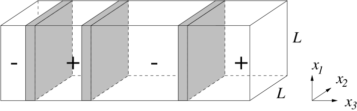
Figure 4: A typical, dominating 3-kink-contribution to the transition amplitude (83) of the matrix element $\langle\,+|{\rm e}^{-HT}|-\,\rangle$ at a temperature just below the critical one. Shaded regions show the location of the kink, the $\pm$-signs in between the adopted vacuum state.

As shown in Fig. 4, one has to take into account that the system can tunnel several times between the two states $|+\,\rangle$ and $|-\,\rangle$, and in the WKB approximation, each of these tunneling processes will (when only tunneling takes long enough because of a sufficient barrier height) contribute to the functional integral a factor

$$K{\rm e}^{-S_{c}}T\,.$$ (87)

The factor $K$ can be calculated, but I shall not discuss it here.

Therefore, having to cross an even (odd) number of interfaces in time development from a state $|+\,\rangle$ ($|-\,\rangle$) to $|+\,\rangle$, one can estimate (81) by

$$\langle\,+|{\rm e}^{-HT}|\pm\,\rangle \sim \sum\limits_{n\;{\rm even(odd)}}K^{n}{\rm e}^{-nS_{c}}\frac{T^{n}}{n!}=$$ (88)

$$=\exp\left(K{\rm e}^{-S_{c}}T\right)\pm\exp\left(-K{\rm e}^{-S_{c}}T\right)\,.$$

The factor $T^{n}/n!$ comes from integration over all different locations of the kinks, i.e. taking into account double counting. Comparison with (81) indeed shows now (82),

$$E_{0A}=K{\rm e}^{-S_{c}}=C{\rm e}^{-\sigma L^{2}}$$ (89)

in $3$ dimensions, so that one knows now how to obtain the interface tension in the finite volume: It can be calculated from the energy splitting between the ground state and the first excited state. For $L\to\infty$, $E_{0A}\to 0$ and spontaneous symmetry breaking is possible, all tunneling processes being exponentially suppressed. In the following, we adopt (89) as definition of the interface tension in field theory.

3.3 Calculating $R_{+}$ in Field Theory

This section outlines the work of references [18] and [19]. In three-dimensional field theory, the coupling $g_{0}$ has a positive mass dimension and – albeit the theory is hence super-renormalisable – infrared divergencies forbid one to construct the critical, i.e. massless, theory perturbatively. One way out is to consider the theory in $4-\epsilon$ dimensions and extrapolate to the case $\epsilon=1$, but it was this technique which led to the unacceptable value of $R_{+}=0.20$ in an ${\cal O}(\epsilon^{2})$-calculation [13]. Also it turned out that convergence was very poor, the ${\cal O}(\epsilon)$-calculation giving $R_{+}=0.14$.

Another technique [11], [20] made renormalisation group calculations in $d=3$ possible by renormalised perturbation theory: Adopting a renormalisation scheme in which the renormalised coupling is denoted $g_{R}$, the perturbative expansion goes in terms of the renormalised, dimensionless variable

$$u_{R}:=\frac{g_{R}}{m_{R}}\,.$$ (90)

Renormalised expansions in terms of $u_{R}$ do not show an infrared problem since even at the critical point, where $m_{R}\to 0$, $u_{R}\to u_{R}^{*}$ remains finite. Thus, information about the critical theory can be obtained by perturbation theory at $u_{R}^{*}$, but $u_{R}$ is not a parameter but fixed by the fixed point value $u_{R}^{*}$, neither is it small.

In our case we choose the renormalised coupling as

$$g_{R}:=3\frac{m_{R}^{2}}{v_{R}^{2}}\,.$$ (91)

The fixed point value of $u_{R}$ is then

$$u_{R}^{*}=15.1\pm 1.3$$ (92)

from various analytical results in the literature.

Clearly, as one approaches the fixed point, i.e. the point of transition between mixed and separated phase, the interface tension vanishes and quantum fluctuations should become important. They are the large entropy fluctuations of statistical mechanics. The saddle point approximation of the functional integral takes into account the quadratic fluctuations about the classical kink solution (85)

$$\Phi({\bf x}) = \Phi_{c}({\bf x})+\eta({\bf x})$$

$$\rightarrow S=S_{c}+\frac{1}{2}\int d^{3}x\;\left[\eta({\bf x})\,M\,\eta({\bf x})+{\cal O}(\eta^{3})\right]$$ (93)

with

$$M=-\partial_{\mu}\partial^{\mu}+m_{0}^{2}-\frac{3}{2}m_{0}^{2}\cosh^{-2}\frac{m_{0}}{2}(x_{3}-a)$$ (94)

and corresponds to a one-loop perturbative calculation.

The (lengthy) calculation is for the two-dimensional case outlined in Coleman’s lectures [14], and in the three-dimensional case it has been performed in Ref. [19]. The result is that the fluctuations modify the energy of the antisymmetric state to

$$E_{0A}=2\left(\frac{S_{c}^{1/2}}{2\pi}\right)\left|\frac{\det^{\prime}M}{\det M_{0}}\right|^{-1/2}\;{\rm e}^{-S_{c}}\,,$$ (95)

where

$$M_{0}=-\partial_{\mu}\partial^{\mu}+m_{0}^{2}\,,$$ (96)

and all contributions from multi-kink configurations have again been taken into account. Because $M$ has zero eigenvalues corresponding to translations of the kink in time (parameter $a$), the determinant of $M$ is calculated without the zero modes, as indicated by the prime over the determinant. The zero modes have to be treated separately by the method of collective coordinates [21] and give rise to the factor $S_{c}^{1/2}\propto L$.

The determinant can be calculated exactly for flat interfaces using heat kernel and $\zeta$-function techniques [18]. Three types of contributions of the final result are worth noting: First, it produces the counter-terms which are required to convert the unrenormalised parameters $m_{0}\,,\,g_{0}\,,\,v_{0}$ of (85) into renormalised ones, giving secondly an additional factor $1/L$. Finally, it gives a substantial one-loop correction to the term proportional to $L^{2}$ in the exponent, and hence to the interface tension (89).

Omitting the details of the calculation of the determinant as well, one arrives by comparison with (89) at an interface tension $\sigma$, which has a negligible, exponentially small $L$-dependence and is in the infinite volume limit given by a Laurent series in $u_{R}$, namely

$$\sigma=2\frac{m^{2}}{u_{R}}\left[1-\frac{u_{R}}{4\pi}\left(\frac{39}{32}-\frac{15}{16}\ln 3\right)+{\cal O}(u_{R}^{2})\right]\,.$$ (97)

Comparison with the tree level result (86) shows that the correction is not negligible. With (3.1/68/69) and (76), one finally obtains

$$R_{-} = \sigma\left(\xi^{-}\right)^{2}=\sigma_{0}\left(\xi^{-}_{0}\right)^{2}=$$

$$= \frac{2}{u_{R}^{*}}\left[1-\frac{u_{R}^{*}}{4\pi}\left(\frac{39}{32}-\frac{15}{16}\ln 3\right)+{\cal O}(u_{R}^{*2})\right]$$

$$= 0.1024\pm 0.0088\,.$$

The one-loop contribution amounts to $22\%$ of the leading term.

As noted at the beginning, experimentalists have measured $R_{+}$, i.e. above the critical temperature, while we calculated $R$ below $T_{c}$, but with the help of another universal quantity, the conversion factor [22]

$$\frac{\xi_{0}^{+}}{\xi_{0}^{-}}=1.96\pm 0.03\,,$$ (99)

one finally obtains

$$R_{+}=0.39\pm 0.03$$ (100)

in good agreement with the experimental value (70). A more recent calculation of my Diplom-student Siepmann gave $u_{R}^{*}=14.73\pm 0.14$, leading to $R_{-}=0.1057\pm 0.0010$. This number is in excellent agreement with recent Monte Carlo calculations by Hasenbusch, Pinn and coworkers [23], which resulted in

$$R_{-}=0.1056\pm 0.0019\,.$$ (101)

References

- [1] R. Haag, Local Quantum Physics, Springer, 1992.
- [2] C. Itzykson, J.-B. Zuber, Quantum Field Theory, McGraw-Hill, 1980.
- [3] L.H. Ryder, Quantum Field Theory, Cambridge University Press, 1989.
- [4] R.F. Streater, A.S. Wightman, PCT, Spin and Statistics, and All That, W.A. Benjamin, 1964.
- [5] J. Glimm, A. Jaffe, Quantum Physics, Springer, 1981.
- [6] K. Osterwalder, R. Schrader, Comm. Math. Phys. 31 (1973) 83; K. Osterwalder, R. Schrader, Comm. Math. Phys. 42 (1975) 281; K. Osterwalder, Euclidean Green’s Functions and Wightman Distributions, in: Constructive Quantum Field Theory, ed. G. Velo and A.S. Wightman, Lecture Notes in Physics 25, Springer, 1973.
- [7] I. Montvay, G. Münster, Quantum Fields on a Lattice, Cambridge University Press, 1994.
- [8] G. Roepstorff, Pfadintegrale in der Quantenphysik, Vieweg Verlag, 1991.
- [9] N. Goldenfeld, Lectures on Phase Transitions and the Renormalization Group, Frontiers in Physics Vol. 85, Addison-Wesley, 1992.
- [10] B. Widom, in: Phase Transitions and Critical Phenomena, Vol. 2, eds. C. Domb and M.S. Green, Academic Press, 1971.
- [11] J.-C. Le Guillou, J. Zinn-Justin, Phys. Rev. B21 (1980) 3976.
- [12] K.K. Mon, Phys. Rev. Lett. 60 (1988) 2749.
- [13] E. Brézin, S. Feng, Phys. Rev. B29 (1984) 472.
- [14] S. Coleman, Aspects of Symmetry, chapter 7, Cambridge University Press, 1985.
- [15] M.E. Fisher, J. Phys. Soc. Japan Suppl. 26 (1969) 87.
- [16] V. Privman, M.E. Fisher, J. Stat. Phys. 33 (1983) 385.
- [17] E. Brézin, J. Zinn-Justin, Nucl. Phys. B257[FS14] (1985) 867.
- [18] G. Münster, Nucl. Phys. B324 (1989) 630.
- [19] G. Münster, Nucl. Phys. B340 (1990) 559.
- [20] G.A. Baker, B.G. Nickel, D.I. Meiron, Phys. Rev. B17 (1978) 1365.
- [21] J.L. Gervais, B. Sakita, Phys. Rev. D11 (1975) 2943.
- [22] H.B. Tarko, M.E. Fisher, Phys. Rev. B11 (1975) 1217; E. Brézin, J.-C. Le Guillou, J. Zinn-Justin, Phys. Lett. A47 (1974) 285.
- [23] M. Hasenbusch, K. Pinn, Physica A192 (1993) 342; M. Caselle, R. Fiore, F. Gliozzi, M. Hasenbusch, K. Pinn, S. Vinti, Nucl. Phys. B432 (1994) 550; V. Agostini, G. Carlino, M. Caselle, M. Hasenbusch, preprint hep-lat/9607029.