The Dirac-Maxwell Equations with Cylindrical Symmetry

Abstract

A reduction of the Dirac-Maxwell equations in the case of static cylindrical symmetry is performed. The behaviour of the resulting system of o.d.e.s is examined analytically and numerical solutions presented. There are two classes of solutions.

• The first type of solution is a Dirac field surrounding a charged “wire.” The Dirac field is highly localised, being concentrated in cylindrical shells about the wire. A comparison with the usual linearized theory demonstrates that this localisation is entirely due to the non-linearities in the equations which result from the inclusion of the “self-field”.

• The second class of solutions have the electrostatic potential finite along the axis of symmetry but unbounded at large distances from the axis.

1 Introduction

This paper is concerned with the system of partial differential equations known as the Dirac-Maxwell equations; the Dirac field describing spin-half matter and the Maxwell field mediating the electromagnetic interactions of the Dirac field. In an earlier paper, [1], one of us (C.J.R.) used the two-spinor formalism to rewrite the equations in a novel way. In fact the electromagnetic potential can be eliminated from the equations altogether. (For further background into the two-spinor formulation of the Dirac equation, see [2]).

In [1] a reduction of the equations was performed in the static case (see section 2, below) and a signifigantly simplified set of (nonlinear) p.d.e.s presented. Finally, after imposing spherical symmetry, the equations were solved (numerically, at least). Unusual features to emerge from that investigation were the existence of highly compact objects and a magnetic monopole. In the present paper we will solve (numerically) the cylindrically symmetric, static Dirac-Maxwell equations. In this case we find no monopole-like solutions. Perhaps this is not unexpected, since there is slightly more regularity in a cylindrical system as opposed to a spherical system – $\ln(r)$ behaviour as distinct from $1/r$ behaviour. However, we do find highly localised solutions – cylindrical shells about a central charged “wire”. When we compare this to the Dirac field solved in an external potential of the same type, no such localisation is apparent.

The cylindrical reduction is also distinguished from the spherical case by the existence of unbounded solutions – solutions in which the Maxwell potential is unbounded at large distances from the symmetry axis. These solutions are also unbounded in the total charge (per unit length of “wire”).

Very few explicit solutions to the full Dirac-Maxwell equations are known and all of these are numerical solutions (or partly so) – see [1], [3] and [4]. Work on the existence theory has progressed steadily, with some important recent work (see [5] and [6]) providing local existence for soliton like solutions.

The solutions in [1] and those presented here show that these equations are capable of representing highly localised structured, entities. Such behaviour is not even hinted at when one examines the usual linearised theory (see section5.2), in which one ignores the Dirac current as a source for the Maxwell field.

2 The Static Dirac-Maxwell Equations

The Dirac-Maxwell equations in standard notation are,

$$\gamma^{\alpha}(\partial_{\alpha}-ieA_{\alpha})\psi+im\psi=0,\;\;\;\;\mbox{where}\;\;\;\;\alpha=0,\ldots,3$$ (1)

$$\mbox{and}\;\;\;\;\partial^{\alpha}F_{\alpha\beta}=-4\pi ej_{\beta},$$ (2)

$$\mbox{where}\;\;\;\;F_{\alpha\beta}=A_{\beta,\alpha}-A_{\alpha,\beta}$$

with the current density given by

$$j_{\alpha}=\overline{\psi}\gamma_{\alpha}\psi.$$

Following [cjr] we use the $\gamma_{5}$ diagonal or van der Waerden description (2-spinor notation, see [2]). The Dirac 4-spinor (or bispinor) is

$$\psi=\left(\begin{array}[]{c}u_{A}\\ \bar{v}^{\dot{B}}\end{array}\right)\;\;\;\;\;\mbox{and}\;\;\;\;\;\overline{\psi}=\left(v^{B},\bar{u}_{\dot{A}}\right).$$

The Dirac equations are

$$(\partial^{A\dot{A}}-ieA^{A\dot{A}})u_{A}+\frac{im}{\sqrt{2}}\bar{v}^{\dot{A}} = 0$$

$$(\partial^{A\dot{A}}+ieA^{A\dot{A}})v_{A}+\frac{im}{\sqrt{2}}\bar{u}^{\dot{A}} = 0.$$ (3)

In [cjr] it was shown that these equations can be solved for the electromagnetic potential, provided the 2-spinors meet a non-degeneracy condition, $u^{A}v_{A}\neq 0$. The result is,

$$A^{A\dot{A}}=\frac{i}{e(u^{C}v_{C})}\left(v^{A}\partial^{B\dot{A}}u_{B}+u^{A}\partial^{B\dot{A}}v_{B}+\frac{im}{\sqrt{2}}(u^{A}\bar{u}^{\dot{A}}+v^{A}\bar{v}^{\dot{A}})\right).$$ (4)

We are interested in the classical Dirac-Maxwell equations, so we will also require that $A^{A\dot{A}}$ is a real vector field (see [cjr]). This leads to the following first order differential equations for $u_{A}$ and $v_{A}$ (“reality conditions”):

$$\partial^{A\dot{A}}(u_{A}\bar{u}_{\dot{A}}) = -\frac{im}{\sqrt{2}}(u^{C}v_{C}-\bar{u}^{\dot{C}}\bar{v}_{\dot{C}})$$

$$\partial^{A\dot{A}}(v_{A}\bar{v}_{\dot{A}}) = \frac{im}{\sqrt{2}}(u^{C}v_{C}-\bar{u}^{\dot{C}}\bar{v}_{\dot{C}})$$

$$u_{A}\partial^{A\dot{A}}\bar{v}_{\dot{A}}-\bar{v}_{\dot{A}}\partial^{A\dot{A}}u_{A} = 0.$$ (5)

The expression for the potential (6), the reality conditions (7) and the Maxwell equations (2), now constitute the full set of nonlinear partial differential equations for the Dirac-Maxwell system. We still have, of course, the $U(1)$ gauge freedom,

$$\begin{array}[]{l}u_{A}\rightarrow e^{i\zeta}u_{A}\\ v^{A}\rightarrow e^{-i\zeta}v^{A}\\ A_{\alpha}\rightarrow A_{\alpha}+\frac{1}{e}\partial_{\alpha}\zeta,\;\;\;\;\,\mbox{a direct consequence of (6).}\end{array}$$

Following [cjr] we now impose the static condition: there exists a Lorentz frame in which there is no current “flow”, $j^{\alpha}=\delta^{\alpha}_{0}j^{0}$ . Under this condition we have

$$v^{A}=e^{i\chi}\sqrt{2}\sigma^{0A\dot{A}}\bar{u}_{\dot{A}}\ ,$$ (6)

where $\chi$ is an arbitrary real function and $\sigma^{\alpha A\dot{A}}$ are the three Pauli matrices with the $2\times 2$ identity matrix as the zeroth $\sigma$ matrix (van der Waerden symbols).

The gauge can be fixed by the choice

$$u^{0} = Xe^{\frac{i}{2}(\chi+\eta)}$$

$$u^{1} = Ye^{\frac{i}{2}(\chi-\eta)}\ ,$$ (7)

where $\eta$, $X$ and $Y$ are real functions.

The static Dirac-Maxwell equations can now be written down, we follow [cjr] and write them in 3-vector notation. This is done by first introducing vectors $V$ and $A$,

$$\begin{array}[]{l}{\mbox{\boldmath$V$}}=(2XY\cos\eta,\,2XY\sin\eta,\,X^{2}-Y^{2})\\ {\mbox{\boldmath$A$}}=(A^{1},A^{2},A^{3}),\,\mbox{where}\,A^{j}=\sigma^{j}_{B\dot{B}}A^{B\dot{B}}\ .\end{array}$$

Our Maxwell-Dirac equations are now given as follows.
The electromagnetic potential is

$$A^{0} = \frac{m}{e}\cos\chi+\frac{(X^{2}-Y^{2})}{2e(X^{2}+Y^{2})}\frac{\partial\eta}{\partial t}+\frac{({\mbox{\boldmath$\nabla$}}\chi){\mbox{\boldmath$.$}}{\mbox{\boldmath$V$}}}{2e(X^{2}+Y^{2})}$$

$$A = \frac{1}{2e(X^{2}+Y^{2})}\left[\frac{\partial\chi}{\partial t}{\mbox{\boldmath$V$}}+(X^{2}-Y^{2}){\mbox{\boldmath$\nabla$}}\eta-{\mbox{\boldmath$\nabla$}}\times{\mbox{\boldmath$V$}}\right].$$ (8)

The reality conditions are

$$\frac{\partial}{\partial t}(X^{2}+Y^{2}) = 0$$ (9)

$$\nabla V = -2m(X^{2}+Y^{2})\sin\chi$$. (10)

$$\frac{\partial{\mbox{\boldmath$V$}}}{\partial t}+\left({\mbox{\boldmath$\nabla$}}\chi\right)\times{\mbox{\boldmath$V$}} = {\boldmath 0}.$$ (11)

Together with the Maxwell equations for $A$ with current vector $j$, as above.

3 Cylindrical Symmetry

The Dirac field given by the 2-spinors $u_{A}$ and $v^{A}$ determines two gauge invariant null vectors $l^{\alpha}=\sigma^{\alpha A\dot{A}}u_{A}\bar{u}_{\dot{A}}$ and $n^{\alpha}=\sigma^{\alpha A\dot{A}}v_{A}\bar{v}_{\dot{A}}$. In fact,

$$(l^{\alpha})=\frac{1}{\sqrt{2}}\left(X^{2}+Y^{2},{\mbox{\boldmath$V$}}\right)\,\;\;\mbox{and}\,\;\;(n^{\alpha})=\frac{1}{\sqrt{2}}\left(X^{2}+Y^{2},-{\mbox{\boldmath$V$ }}\right),$$

assuming that the field is static. Note that the current vector $j^{\alpha}=l^{\alpha}+n^{\alpha}$. The first reality condition tells us that the zeroth component of $l^{\alpha}$ and $n^{\alpha}$ are independent of time. We also assume that $l^{\alpha}$ and $n^{\alpha}$ are independent of $z$ in keeping with the assumption of cylindrical symmetry. Here $(\rho,\phi,z)$ are the cylindrical polar coordinates corresponding to our original Cartesian coordinates.

Applying these conditions one finds that $\eta=\phi$, $X=X(\rho)$ and $Y=Y(\rho)$. The second of the reality conditions then implies that $\chi=\chi(\rho)$. The third reality condition then gives

$$(X^{2}-Y^{2})\frac{d\chi}{d\rho}=0.$$

If we take $\chi=constant$ then we find $A^{0}=constant$, the Maxwell equation then implies that $X=Y=0$. However, the non-degeneracy condition, $u^{A}v_{A}\neq 0$, excludes this possibility. So we assume $\chi^{\prime}(\rho)\neq 0$ from now on and consequently, $X=Y$. Our equation for the electromagnetic potential (8), shows that the vector potential $A$ vanishes. There is no magnetic monopole, as distinct from the spherical case.

The equations now simplify to the following ordinary differential equations:

$$A_{0} = \frac{m}{e}\cos\chi+\frac{1}{2e}\frac{d\chi}{d\rho}$$

$$\frac{d}{d\rho}\left(\rho X^{2}\right) = -2m\rho X^{2}\sin\chi$$

$$\frac{d}{d\rho}\left(\rho\frac{dA_{0}}{d\rho}\right) = 8\pi\sqrt{2}eX^{2}\rho.$$ (12)

Introducing dimensionless variables

$$A = \frac{e}{m}A_{0}$$

$$\hat{\rho} = 2m\rho$$

$$Z = \frac{8\pi\sqrt{2}\rho e^{2}}{m^{2}}X^{2}.$$

From here on we will refer to $\hat{\rho}$ as $\rho$ for the sake of simplicity. We also define a new dependent variable

$$F=\rho\frac{dA}{d\rho},$$

so that we get a system of four first order equations

$$(a)\;\;\;\;\;\;\frac{d\chi}{d\rho} = A-\cos\chi$$

$$(b)\;\;\;\;\;\;\frac{dF}{d\rho} = Z$$

$$(c)\;\;\;\;\;\;\frac{dA}{d\rho} = \frac{F}{\rho}$$

$$(d)\;\;\;\;\;\;\frac{dZ}{d\rho} = -Z\sin\chi.$$ (13)

The equations can also be written as a fourth order equation in the dependent variable $\chi$:

$$\frac{d^{2}}{d\rho^{2}}\left(\rho\left(\frac{d^{2}\chi}{d\rho^{2}}-\sin\chi\frac{d\chi}{d\rho}\right)\right)+\frac{d}{d\rho}\left(\rho\left(\frac{d^{2}\chi}{d\rho^{2}}-\sin\chi\frac{d\chi}{d\rho}\right)\right)\sin\chi=0.$$ (14)

Much of the qualitative behaviour of solutions to our system will be determined by the behaviour of the dependent variables in the vicinity of the two singular points $\rho=0$ and $\rho=\infty$.

4 Behaviour Near $0$ And $\infty$

The variable $Z$ is the charge density which we assume to be non-negative (In fact, it is straightforward to show that $Z\geq 0=>Z>0$. See proof of Lemma $2$.) $F$ is the integral of the charge $Z$ per unit ring, that is, $F(\rho)-F(0)$ is the total charge within a radius $\rho$. It is reasonable, therefore, to restrict our attention to solutions where $F$ remains bounded as $\rho$ approaches $\infty$. Much of the behaviour of the solution can be characterised by the values of $F$ at either end of the domain. This behaviour can best be summarized in the following two Lemmas.

Lemma 1

Suppose $(\chi,F,A,Z)$ is a solution to Equation(13) on $I=(0,\rho_{1})$, for some $\rho_{1},0<\rho_{1}<1$. Suppose also that $Z\geq 0$ is continuous and bounded on $I$. Then,

1. $F$ is $C^{1}$ on I and has a well defined, finite limit as $\rho\rightarrow 0$. $Z$ has a well-defined limit as $\rho\rightarrow 0$.

2. if $F(0)\neq 0$ then $A$ is unbounded as $\rho\rightarrow 0$. In particular, $A=\Omega(\rho)\ln(\rho)$, where $\Omega$ is $C^{2}$ and bounded on I, $\Omega\rightarrow F(0)$ as $\rho\rightarrow 0$. Also, $\chi$ is bounded as $\rho\rightarrow 0$.

Proof

1. Let $0<\rho_{1}<\rho_{2}<1$.
   From $(c)$ , $\frac{dF}{d\rho}=Z$, so $F$ is $C^{1}$ and $|F(\rho_{2})-F(\rho_{1})|\leq M(\rho_{2}-\rho_{1})$ where $M=sup_{I}Z$.
   Letting $\rho_{1},\rho_{2}\rightarrow 0$ shows that $F$ has a well-defined limit. Fixing $\rho_{2}$, and letting $\rho_{1}\rightarrow 0$ shows that this limit is finite. A similar argument using (d); $\frac{dZ}{d\rho}=-Z\sin{\chi}\leq M$, shows that $Z$ has a well-defined limit.

2. Let $A=\Omega\ln\rho$. $A$ is $C^{2}$ on $I$ since, from (c), $\frac{dA}{d\rho}=\frac{F}{\rho}$; therefore $\Omega$ is $C^{2}$. We also have

   $$F=\rho\ln\rho\frac{d\Omega}{d\rho}+\Omega$$ (15)

   and

   $$\frac{d}{d\rho}\left(\rho(\ln\rho)^{2}\frac{d\Omega}{d\rho}\right)=Z\ln\rho.$$ (16)

   From (16), (since $\ln\rho<0$ on $I$),

   $$M\ln\rho\leq\frac{d}{d\rho}\left(\rho(\ln\rho)^{2}\frac{d\Omega}{d\rho}\right)\leq 0.$$

   Integrating,

   $$M\left(\rho_{1}(\ln\rho_{1}-1)-\rho(\ln\rho-1)\right)\leq c_{1}-\rho(\ln\rho)^{2}\frac{d\Omega}{d\rho}\leq 0,$$

   where

   $$c_{1}=\rho_{1}(\ln\rho_{1})^{2}\frac{d\Omega}{d\rho}(\rho_{1}).$$

   That is,

   $$\frac{M\left(\rho_{1}(\ln\rho_{1}-1)-\rho(\ln\rho-1)\right)}{\ln\rho}\leq\rho\ln\rho\frac{d\Omega}{d\rho}\leq\frac{c_{1}}{\ln\rho}.$$

   Letting $\rho\rightarrow 0$, we see that $\rho\ln\rho\frac{d\Omega}{d\rho}\rightarrow 0$. Hence, from (15) we see that $\Omega\rightarrow F(0)$ as $\rho\rightarrow 0$.

   Now, since $\Omega$ is bounded on $I$ put $c_{2}\leq\Omega\leq c_{3}$, for some constants $c_{2}$ and $c_{3}$. From (a),

   $$A-1\leq\frac{d\chi}{d\rho}\leq A+1.$$

   Thus,

   $$c_{2}\ln\rho-1\leq\frac{d\chi}{d\rho}\leq c_{3}\ln\rho+1.$$

   Integrating, we have

   $$\chi(\rho) \leq \chi(\rho_{1})+c_{2}\left(\rho_{1}(\ln\rho_{1}-1)-\rho(\ln\rho-1)\right)-(\rho_{1}-\rho)$$

   $$\chi(\rho) \geq \chi(\rho_{1})+c_{3}\left(\rho_{1}(\ln\rho_{1}-1)-\rho(\ln\rho-1)\right)+(\rho_{1}-\rho),$$

   which bounds $\chi(\rho)$ as $\rho\rightarrow 0$.

   $\Box$

Lemma 2

Suppose $(\chi,F,A,Z)$ is a solution to Equation(13) on $\rho\in(0,\infty)$. Suppose also that $Z\geq 0$ with $F$ continous and bounded on the interval. Then

1. If $F(\rho_{1})\geq 0$ for some $\rho_{1}\in\left[0,\infty\right)$, then $\chi\rightarrow\infty$, $A\rightarrow\infty$, and $F\rightarrow\infty$ as $\rho\rightarrow\infty$.

2. If $F<0$ on $(0,\infty)$ then $F\rightarrow 0$ as $\rho\rightarrow\infty$. In addition, if $A$ and $Z$ have well-defined limits as $\rho\rightarrow\infty$ then $Z\rightarrow 0$ and $A\rightarrow A_{\infty}$ as $\rho\rightarrow\infty$, with $-1\leq A_{\infty}\leq 1$.

Proof

1. We firstly show that, given the nondegeneracy condition, $u^{A}v_{A}\neq 0$ a.e., that $Z\geq 0=>Z>0$ for all $\rho\in I$. Suppose $Z(\rho_{1})=0$ for some $\rho_{1}\in I$. Now $\frac{d}{d\rho}(Ze^{\rho})\geq 0$, using (d). Integrating from $\rho$ to $\rho_{1}\left(\rho\in(0,\rho_{1})\right)$, shows that $Z(\rho)=0$ for all $\rho\in(0,\rho_{1})$. A similar argument using $\frac{d}{d\rho}(Ze^{-\rho})\leq 0$ shows that $Z(\rho)=0$ for all $\rho\in(\rho_{1},\infty)$. Thus, if $Z(\rho_{1})=0$, then $Z\equiv 0$ on $I$. But this possibility is excluded by the non-degeneracy condition. Therefore, $Z>0$ on $(0,\infty)$. This shows that $Z$ does not have isolated zeroes.

   $F$ is (strictly) monotonic increasing everywhere, since from (b) $\frac{dF}{d\rho}=Z$ and $Z>0$. If $F(\rho_{1})\geq 0$ for some $\rho_{2}>\rho_{1}$, $F(\rho_{2})>0.$ So, for $\rho\in(\rho_{2},\infty)$

   $$\frac{dA}{d\rho}=\frac{F}{\rho}\geq\frac{F(\rho_{2})}{\rho}.$$

   Integrating,

   $$A(\rho)\geq A(\rho_{2})+F(\rho_{2})\ln\left(\frac{\rho}{\rho_{2}}\right)$$

   and $A\rightarrow\infty$ as $\rho\rightarrow\infty$.

   Also, from (a), $\frac{d\chi}{d\rho}\geq A-1$, which implies, after integration, that $\chi\rightarrow\infty$ as $\rho\rightarrow\infty$.

   Now on $(\rho_{2},\infty)$, $F$ is bounded below by $F(\rho_{2})$. Let us assume that $F$ is bounded above, i.e. $0<F(\rho_{2})\leq F(\rho)\leq\beta$, a constant. Consider

   $$\frac{d}{d\rho}\left(\frac{Z(A-\cos\chi)}{A+1}\right)=\frac{ZF(1+\cos\chi)}{\rho(A+1)^{2}}.$$ (17)

   Now for $\rho_{2}$ large enough, $A>1$ on $(\rho_{2},\infty)$ and so

   $$\frac{Z(A-\cos\chi)}{A+1}\;\;>\;\;c_{4}\;\;=\;\;\frac{Z(\rho_{2})\left(A(\rho_{2})-\cos\chi(\rho_{2})\right)}{A(\rho_{2})+1}>0.$$

   Thus,

   $$Z(A-\cos\chi)>c_{4}(A+1).$$ (18)

   Now consider

   $$V(\rho)=Z(A-\cos\chi)-\frac{F^{2}}{2\rho}-\int^{\rho}_{\rho_{2}}\frac{F^{2}(\sigma)}{2(\sigma^{2}}\,d\sigma.$$

   $\frac{dV}{d\rho}=0$, so $V(\rho)=V(\rho_{2})$, constant on $(\rho_{2},\infty)$. But

   $$V(\rho)\geq Z(A-\cos\chi)-\frac{F(\rho_{2})^{2}}{2\rho}-\frac{1}{2}F(\rho_{2})^{2}\int^{\rho}_{\rho_{2}}\frac{d\sigma}{(\sigma)^{2}},$$

   and so, using (18), since $A\rightarrow\infty$ as $\rho\rightarrow\infty$, then $V(\rho)\rightarrow\infty$ as $\rho\rightarrow\infty$. Clearly $\rho_{2}$ can be chosen at a point where $V(\rho_{2})$ is finite. We have a contradiction. $F$ cannot be bounded by a positive real number. That is, $F\rightarrow\infty$ as $\rho\rightarrow\infty.$

2. We assume there exists a constant $\eta$ s.t. $F(\rho)<\eta<0$ for all $\rho\in(0,\infty)$. Then, since $\frac{dA}{d\rho}=F/\rho$,

   $$A\leq A(\rho_{2})+\eta\ln(\frac{\rho}{\rho_{2}}),$$

   and so $A\rightarrow-\infty$ as $\rho\rightarrow\infty$. Similarly $\chi\rightarrow-\infty$ as $\rho\rightarrow\infty$.

   Now

   $$\frac{d}{d\rho}\left(\frac{Z(A-\cos\chi)}{A-1}\right)=\frac{ZF\left(-1+\cos\chi)\right)}{\rho(A-1)^{2}}\geq 0.$$ (19)

   Therefore

   $$\frac{Z(A-\cos\chi)}{A-1}\geq c_{5}\;\;=\;\;\frac{Z(\rho_{2})\left(A(\rho_{2})-\cos\chi(\rho_{2})\right)}{A(\rho_{2})-1}\geq 0,$$

   for $\rho_{2}$ large enough, since $A\rightarrow-\infty$ as $\rho\rightarrow\infty$. Therefore

   $$Z(A-\cos\chi)\;\;\leq\;\;c_{5}(A-1).$$

   Hence $Z(A-\cos\chi)\rightarrow-\infty$ as $\rho\rightarrow\infty$.

   Now, using a similar argument to that in (i), using $V(\rho)$, we have a contradiction. Hence, $F$ cannot be bound above by $\eta<0$. But $\frac{dF}{d\rho}=Z>0$, thus $F\rightarrow 0$ as $\rho\rightarrow\infty$ (otherwise, we have case (i)). The proof of $Z\rightarrow 0$ as $\rho\rightarrow\infty$ is handled in a similar manner. The bounds on $A_{\infty}$ are also easily established using arguments of this type. For example, assume $A_{\infty}<-1$ and use (17) and (19).

   $\Box$

5 Numerical Solutions

5.1 Charged Wire with Two Dense Rings

As stated in Lemma 2 $(ii)$, if $F<0$ on $I$, then $F\rightarrow 0$ as $\rho\rightarrow\infty$. To obtain a numerical solution of this type, we expand $\chi$ in $\frac{1}{\rho}$ and solve for the coefficients of $\chi,A,F,Z$ as $\rho\rightarrow\infty$. There is only one such solution, the coefficients in the expansions being uniquely determined.

$$\chi = \pi-3\frac{1}{\rho}+\frac{1}{6}\frac{1}{\rho^{3}}-\frac{9247}{67320}\frac{1}{\rho^{5}}+\dots$$

$$A = -1+\frac{15}{2}\frac{1}{\rho^{2}}-\frac{35}{8}\frac{1}{\rho^{4}}+\frac{77425}{26928}\frac{1}{\rho^{6}}+\dots$$

$$F = -15\frac{1}{\rho^{2}}+\frac{35}{2}\frac{1}{\rho^{4}}-\frac{77425}{4488}\frac{1}{\rho^{6}}+\dots$$

$$Z = 30\frac{1}{\rho^{3}}-70\frac{1}{\rho^{5}}+\frac{77425}{748}\frac{1}{\rho^{7}}+\dots\ .$$ (20)

Using these expressions, we evaluate our initial values (near infinity). We used a multistep differential equation solver (from the NAG Fortran Library (Mark 16)[7]), interfaced with MATLAB ([8])). The numerical solution is given in Figure 1.

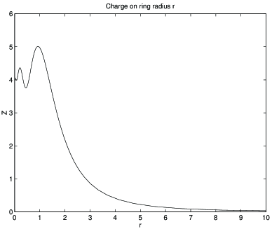
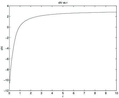
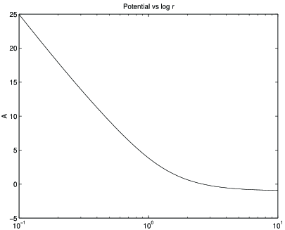
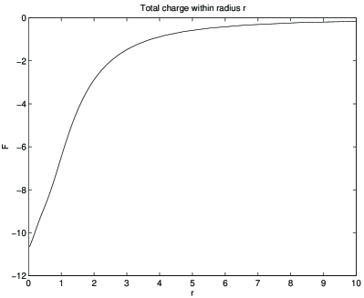
Figure 1: Numerical solutions to the static D-M equations, with cylindrical symmetry

As stated in Lemma 1, $\chi$ remains finite as $\rho\rightarrow 0$. We can calculate the value of $\chi(0)$ numerically: $\chi(0)=-12.17$ noting that $\chi\rightarrow\pi$ as $\rho\rightarrow\infty$. From (d) we have

$$\frac{dZ}{d\rho}=0\;\;\;\;\mbox{when}\;\;\;\;\chi=n\pi.$$

From Figure 1 we see that $\chi$ is monotonic and bounded between $-4\pi$ and $\pi$. $Z$ has four critical points for $\rho\in(0,\infty)$. These occur successively as maxima and minima. $Z$ has two finite values of $\rho$, $\rho_{1}$ and $\rho_{2}$, say, for which the charge density is a local maximum. See Figure 1. Numerically, after converting to units, in which $\rho$ is measured in $\lambda_{C}=\frac{1}{m}$, the reduced Compton wavelength, $\rho_{1}\approx.12\lambda_{C}$, and $\rho_{2}\approx.46\lambda_{C}$. In the full three-dimensional picture, this corresponds to two densely charged rings around the $z$ axis.

Plotting $A$ against $\ln\rho$, in the inner region (inside the dense rings) we obtain a linear plot, in keeping with Lemma 1($ii$):

$$A\approx F(0)\ln\rho\;\;\;\;\mbox{for}\;\;\;\;\rho<<\rho_{1}.$$

This is just the standard cylindrically symmetric solution to vacuum Maxwell equations – the potential due to a charged wire (along the $z$ axis). Note that, $F(0)=\frac{146}{\lambda_{C}}$ corresponding to a charge per Compton wavelength of $146e$. Coupling the Maxwell and Dirac equations, then, has the effect of surrounding the charged wire with two dense rings of charge.

5.2 Comparison with the Linearized Theory

In this section we consider, by way of comparison, the solution to the Dirac equation in an external field generated by a charged wire. We now use the decoupled equations, i.e. the Dirac equation with the vacuum Maxwell equation.

In the static cylindrically symmetric case, the solution to the vacuum Maxwell equation is $A=c_{0}\ln\rho.$ Using the same notation as in the previous section, we choose $c_{0}=F(0)<0$. We can now solve the Dirac equation, using this (external) potential. Our equations are

$$(a)\;\;\;\;\;\;\frac{d\chi}{d\rho} = -10.79\ln\rho-\cos\chi$$

$$(b)\;\;\;\;\;\;\frac{dZ}{d\rho} = -Z\sin\chi.$$ (21)

For comparison purposes, we solve these linearized equations with the same initial conditions used for our earlier solution. The numerical solution was obtained using the same methods as in the previous section and are shown in Figure 2.

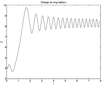
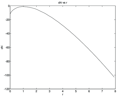
Figure 2: Numerical solution to the Dirac equation aound a charged wire, treated as an external field

For small values of $\rho$ the current density, $Z$, behaves in a similar manner (to the solution of the non-linearised D-M equations), having the first peak at $\rho_{1}\approx.11\lambda_{C}$. As $\rho\rightarrow\infty$ the (logarithmic) potential is unbounded, in contrast to the nonlinearised case, in which $-1\leq A_{\infty}\leq 1$ (see Lemma 2). It is clear from equation (21$(a)$) that $\chi\rightarrow-\infty$ as $\rho\rightarrow\infty$. As such, (from 21$(b)$), there will be an infinite number of oscillations in the charge density variable $Z$, which, however, remains bounded. We have lost the localization that was apparent in the full D-M equations.

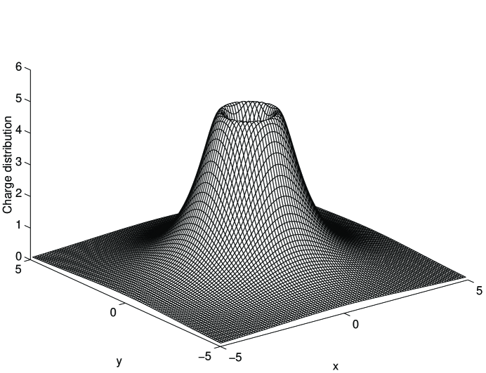
Figure 3: Charge distribution of the Dirac-Maxwell field with cylindrical symmetry evidencing a highly localised charge density around a central charged wire. Total charge (per unit length) is finite.

Figure 4: Charge distribution of the Dirac equation surrounding a charged wire, treated as an external field. No localisation of the charge distribution is apparent. The total charge (per unit length) is unbounded.

5.3 Unbounded Solutions

As stated in Lemma 1$(ii)$, if $F(0)\neq 0$ then $A$ is unbounded as $\rho\rightarrow 0$. We can also look for solutions where $F(0)=0$. Lemma 2 then tells us that $\chi,A,F\rightarrow\infty$ as $\rho\rightarrow\infty$. Since $F(\rho)$ is the charge within a radius $\rho$, these solutions are of less interest, as the total charge, $F(\infty)$ is necessarily unbounded.

To find a numerical solution of this type, we expand $\chi$ into a Taylor Series in $\rho$ and solve for the coefficients.

As an example of this type of solution we set $A(0)=1$ and $\chi_{0}=0$. The first few terms of these and the remaining variables are given below.

$$\chi = \frac{1}{100}\rho+\frac{1}{100}\rho^{2}+\frac{1}{60000}\rho^{3}+\frac{1}{45000}\rho^{4}+\dots$$

$$A = \frac{101}{100}+\frac{1}{50}\rho-\frac{1}{90000}\rho^{3}-\frac{1}{240000}\rho^{4}+\dots$$

$$F = \frac{1}{50}\rho-\frac{1}{30000}\rho^{3}-\frac{1}{60000}\rho^{4}+\dots$$

$$Z = \frac{1}{50}-\frac{1}{10000}\rho^{2}-\frac{1}{15000}\rho^{3}+\frac{67}{4000000000}\rho^{4}+\dots\ .$$ (22)

In Figure 5 we show the solution which has these initial values.

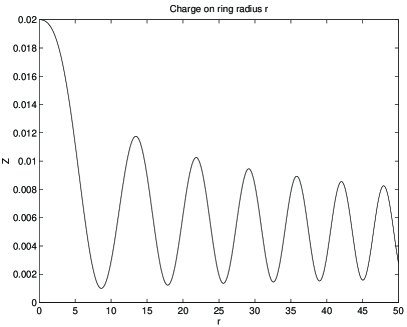
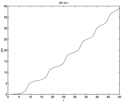
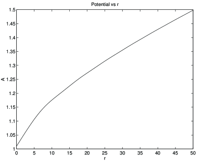
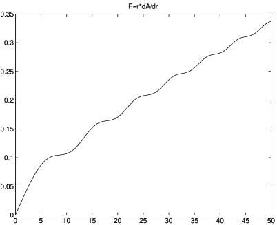
Figure 5: Numerical solutions to the D-M equations, with $F(0)=0$.

6 Conclusions

An examination of the behaviour of the solutions to the static Dirac-Maxwell Equations with cylindrical symmetry shows that, in one class of solution, we have a highly localised charge density around a central charged “wire”. The total charge (per unit length of the “wire”) is finite.

When the equations are decoupled (by ignoring the effect of the “self-field” upon the Maxwell field) all localisation is lost. The total charge (per unit length) of the Dirac field is, in this case, unbounded.

Although the cylindrical case is of limited interest physically, the resulting o.d.e.s are amenable to a detailed descriptive analysis which corrorborates the numerical results.

The same localisation due to the inclusion of a nonlinear coupling, will be more interesting in the axially symmetric case, an analysis of which will be in a forthcoming publication.

7 Acknowledgements

The first named author was partially supported by an Australian Postgraduate Award.

References

- [1] C.J. Radford, Localised Solutions of the Dirac-Maxwell Equations, J. Math. Phys (to appear).
- [2] R. Penrose and W. Rindler, Spinors and Space-Time, Vol. 1, Cambridge Monographs in Mathematical Physics, Cambridge University Press, Cambridge,1992.
- [3] M. Wakano, Intensely Localized Solutions of the Dirac-Maxwell Field Equations, Prog.T.Phys. 35, 1117-1141, (1966).
- [4] A.G. Lisi, A solitary wave solution of the Maxwell-Dirac equations, J.Phys.A 28 No.18, 5385-5392 (1995).
- [5] M. Esteban, V. Georgiev, E. Sere, Stationary Solutions of the Maxwell-Dirac and Gordon-Dirac Equations , preprint 9514, CEREMADE (URA CNRS 749), Universite of Paris Dauphine, (1995).
- [6] M.Esteban, E. Sere, Stationary States of the Nonlinear Dirac Equation: A Variational Approach, Comm. Math. Phys. 171, 323-350, (1995)
- [7] NAG is a registered trademark of The Numerical Algorithms Group, Inc.
- [8] MATLAB is a trademark of The MathWorks, Inc.