On the finite dimensional quantum group

$M_{3}\oplus(M_{2|1}(\Lambda^{2}))_{0}$

R. Coquereaux

Instituto Balseiro - Centro Atomico de Bariloche

CC 439 - 8400 -San Carlos de Bariloche - Rio Negro - Argentina

Centre de Physique Théorique - CNRS - Luminy, Case 907

F-13288 Marseille Cedex 9 - France

We describe a few properties of the non semi-simple associative algebra ${\cal H}\doteq M_{3}\oplus(M_{2|1}(\Lambda^{2}))_{0}$, where $\Lambda^{2}$ is the Grassmann algebra with two generators. We show that ${\cal H}$ is not only a finite dimensional algebra but also a (non co-commutative) Hopf algebra, hence a finite dimensional quantum group. By selecting a system of explicit generators, we show how it is related with the quantum enveloping algebra of $SL_{q}(2)$ when the parameter $q$ is a cubic root of unity. We describe its indecomposable projective representations as well as the irreducible ones. We also comment about the relation between this object and the theory of modular representations of the group $SL(2,F_{3})$, i.e. the binary tetrahedral group. Finally, we briefly discuss its relation with the Lorentz group and, as already suggested by A.Connes, make a few comments about the possible use of this algebra in a modification of the Standard Model of particle physics (the unitary group of the semi-simple algebra associated with ${\cal H}$ is $U(3)\times U(2)\times U(1)$).

anonymous ftp or gopher: cpt.univ-mrs.fr

Keywords: quantum groups, Hopf algebras, standard model, particle physics, non-commutative geometry.

CPT-96/P.3388

On the finite dimensional quantum group $M_{3}\oplus(M_{2|1}(\Lambda^{2}))_{0}$

1 Introduction

Quantum groups – either specialized at roots of unity or not – have been used many times, during the last decade, in the physics of integrable models and in conformal theories [29]. The wish of using such mathematical structures, both nice and new, in four-dimensional particle physics has triggered the imagination of many people in the last years.

When $q$ is a root of unity, there are other interesting objects besides the quantized enveloping algebra itself : some of its finite dimensional subalgebras or some of its finite dimensional quotients may still carry a Hopf algebra structure.

We do not need to mention the importance of finite dimensional classical symmetries in Physics, but it is our belief that finite dimensional quantum symmetries will turn out to be also of prime importance in theories of fundamental interactions –in this respect, one can already mention the relations between quantum symmetries of graphs [27] and the classification of conformal field theories [14].

Such finite dimensional quantum groups are also interesting from the mathematical point of view because they provide examples of finite dimensional Hopf algebras which are neither commutative nor co-commutative : they are a kind of direct “quantum” generalization of discrete groups (or, better, generalizations of the corresponding group algebras). These objects are also interesting because of their —still not totally understood— relations with the theory of modular representations of algebraic groups [20][21].

The fact that the semi-simple part of a finite dimensional quotient of the quantum algebra $U_{q}(SL(2,\mbox{\rm C}\hskip-6.0pt\mbox{l}\;))$, when $q$ is a primitive cubic root of unity, has a unitary group equal to $U(3)\times U(2)\times U(1)$ suggests that this finite quantum group could have something to do with the Standard Model of particle physics. This remark was explicitly made in the framework of non-commutative geometry by Connes in [4] and more recently in [6]. We do not intend, in the present paper, to show how to analyze this finite quantum group along the lines of non-commutative geometry (for a very detailed account of the Standard Model “à la Connes”, not involving quantum groups at all, we refer to the recent papers [25] or [6]).

In order to make use of a symmetry in physics, it is good to be already acquainted with it. It could be tempting to assume that the reader knows already everything about representation theory of non semi-simple algebras, Jacobson radical, quivers, Hopf algebras and other niceties belonging to the toolbox of the perfect algebraist but this would amount to assume that nobody can appreciate the beauty of a tetrahedron before being acquainted with the properties of the exceptional Lie group $E_{6}$. Our point of view is that, since the properties of the algebra ${\cal H}$ can be understood without using anything more sophisticated than basic multiplication or tensor products of matrices as well as elementary calculus involving anti-commuting numbers (Grassmann numbers), it is very useful to study them in this way, at least in a first approach.

We therefore want to present —in very simple terms— the rather nice finite dimensional algebra of quantum symmetries mentioned before, without assuming from the reader any a priori knowledge on quantum groups, general associative algebras and the like. We shall therefore define explicitly this finite dimensional quantum group, as the algebra ${\cal H}\doteq M_{3}\oplus(M_{2|1}(\Lambda^{2}))_{0}$, where $M_{3}$ is the set of $3\times 3$ matrices over the complex numbers, and where $(M_{2|1}(\Lambda^{2}))_{0}$ is the Grassmann envelope of the associative $\mbox{\rm Z}\hskip-4.0pt\mbox{\rm Z}_{2}$ graded algebra $M_{2|1}(\mbox{\rm C}\hskip-6.0pt\mbox{l}\;^{2})$, i.e. , the even part of its graded tensor product with a Grassmann algebra $\Lambda^{2}$ with two generators.

The motivation and underlying belief is, of course, that there should be some quantum symmetry, hitherto unnoticed, in the Standard Model, or, maybe, in a modification of it, symmetry that would, ultimately, cast some light on the puzzle of fermionic families and mass matrices.

The present paper is not only a pedagogical exercise: although several properties that we shall describe have been already discussed in the literature (see in particular [1],[30]), usually using a less elementary language, others do not seem to be published. Sections 2 to 5 are supposed to be elementary and self-contained; the last two sections contain a set of less elementary results and unrelated comments.

Finite dimensional quantum groups associated with quantum universal enveloping algebras can be defined for any type of Lie group, when the parameter $q$ is a primitive root of unity. It is possible to give an explicit realization — in terms of matrices with complex and grassmanian entries — for the other finite quantum groups of $SL(2)$ type when $q$ is a root of the unity (see [10], [28]). Following hopes or claims that such algebras can provide interesting physical models, it seems that there is some need for a paper explaining the basic properties of the simplest non trival quantum group of this type, namely, when $q^{3}=1$. This is the purpose of the present paper. Construction of a “generalized” gauge theory on ${\cal H}$, along the lines of non commutative geometry, is clearly possible but lies beyond the scope of this article.

2 The algebra ${\cal H}\doteq M_{3}\oplus(M_{2|1}(\Lambda^{2}))_{0}$

Let $\Lambda^{2}$ be the Grassmann algebra over Cl  with two generators, i.e. the linear span of $\{1,\theta_{1},\theta_{2},\theta_{1}\theta_{2}\}$ with arbitrary complex coefficients, where the generators satisfy the relations $\theta_{1}^{2}=\theta_{2}^{2}=0$ and $\theta_{1}\theta_{2}=-\theta_{2}\theta_{1}$. This algebra has an even part, generated by $1$ and $\theta_{1}\theta_{2}$ and an odd part generated by $\theta_{1}$ and $\theta_{2}$. We call $M_{3}$ the algebra of $3\times 3$ matrices over the complex numbers and $M_{2|1}$ another copy of this algebra that we grade as follows: A matrix $V\in M_{2|1}$ is called even if it is of the type

$$V=\pmatrix{V_{11}&V_{12}&0\cr V_{21}&V_{22}&0\cr 0&0&V_{33}}$$

and odd if it is of the type

$$V=\pmatrix{0&0&V_{13}\cr 0&0&V_{23}\cr V_{31}&V_{32}&0}$$

We call $(M_{2|1}(\Lambda^{2}))_{0}$ the Grassmann envelope of $M_{2|1}$ which is defined as the even part of the tensor product of $M_{2|1}$ and $\Lambda^{2}$, i.e. the space of matrices $3\times 3$ matrices $V$ with entries $V_{11}$, $V_{12}$, $V_{21}$, $V_{22}$, $V_{33}$, that are even Grassmann elements (of the kind $\alpha+\beta\theta_{1}\theta_{2}$) and entries $V_{13}$, $V_{23}$,$V_{31}$, $V_{32}$ that are odd Grassmann elements (i.e. of the kind $\gamma\theta_{1}+\delta\theta_{2}$). We define ${\cal H}$ as

$${\cal H}\doteq M_{3}\oplus(M_{2|1}(\Lambda^{2}))_{0}$$

Explicitly,

$${\cal H}=\pmatrix{*&*&*\cr*&*&*\cr*&*&*}\oplus\pmatrix{\alpha_{11}+\beta_{11}\theta_{1}\theta_{2}&\alpha_{12}+\beta_{12}\theta_{1}\theta_{2}&\gamma_{13}\theta_{1}+\delta_{13}\theta_{2}\cr\alpha_{21}+\beta_{21}\theta_{1}\theta_{2}&\alpha_{22}+\beta_{22}\theta_{1}\theta_{2}&\gamma_{23}\theta_{1}+\delta_{23}\theta_{2}\cr\gamma_{31}\theta_{1}+\delta_{31}\theta_{2}&\gamma_{32}\theta_{1}+\delta_{32}\theta_{2}&\alpha_{33}+\beta_{33}\theta_{1}\theta_{2}}$$

All entries besides the $\theta$’s are complex numbers (the above $\oplus$ sign is a direct sum sign: these matrices are $6\times 6$ matrices written as a direct sum of two blocks of size $3\times 3$).

It is obvious that this is an associative algebra, with usual matrix multiplication, of dimension $27$ (just count the number of arbitrary parameters). ${\cal H}$ is not semi-simple (because of the appearance of Grassmann numbers in the entries of the matrices) and its semi-simple part $\overline{{\cal H}}$, given by the direct sum of its block-diagonal $\theta$-independent parts is equal to the $9+4+1=14$-dimensional algebra $\overline{{\cal H}}=M(3,\mbox{\rm C}\hskip-6.0pt\mbox{l}\;)\oplus M(2,\mbox{\rm C}\hskip-6.0pt\mbox{l}\;)\oplus\mbox{\rm C}\hskip-6.0pt\mbox{l}\;$. The radical (more precisely the Jacobson radical) $J$ of ${\cal H}$ is the left-over piece that contains all the Grassmann entries, and only the Grassmann entries, so that $\overline{{\cal H}}={\cal H}/J$. $J$ has therefore dimension $13$.

3 A system of generators for ${\cal H}$

Let $q$ be a primitive cubic root of unity ($q^{3}=1$). Hence, $\overline{q}=q^{2}=q^{-1}$ and $1+q+q^{2}=0$. We also set $\lambda=q-q^{-1}$. In order to write generators for ${\cal H}$, we need to consider $6\times 6$ matrices that have a $(3\times 3)\oplus((2|1)\times(2|1))$ block diagonal structure. We introduce elementary matrices $E_{ij}$ for the $M(3,\mbox{\rm C}\hskip-6.0pt\mbox{l}\;)$ part and elementary matrices $F_{ij}$ for the $M(2|1,\mbox{\rm C}\hskip-6.0pt\mbox{l}\;)$ part.

The associative algebra ${\cal H}$ defined previously can be generated by the following three matrices

$$X_{+} = E_{12}+E_{23}+(1-\theta_{1}\theta_{2}/2)F_{12}+\theta_{1}(F_{23}+F_{31})$$

$$X_{-} = -E_{21}-E_{32}+(1-\theta_{1}\theta_{2}/2)F_{21}+\theta_{2}(F_{13}-F_{32})$$

$$K = q^{2}E_{11}+E_{22}+q^{-2}E_{33}+qF_{11}+q^{-1}F_{22}+F_{33}$$

Explicitly, one gets

$$X_{+}\doteq\pmatrix{\pmatrix{0&1&0\cr 0&0&1\cr 0&0&0}&\pmatrix{}\cr\pmatrix{}&\pmatrix{0&1-{\theta_{1}\theta_{2}\over 2}&0\cr 0&0&\theta_{1}\cr\theta_{1}&0&0}}$$

$$X_{-}\doteq\pmatrix{\pmatrix{0&0&0\cr-1&0&0\cr 0&-1&0}&\pmatrix{}\cr\pmatrix{}&\pmatrix{0&0&\theta_{2}\cr 1-{\theta_{1}\theta_{2}\over 2}&0&0\cr 0&-\theta_{2}&0}}$$

$$K\doteq\pmatrix{\pmatrix{q^{2}&0&0\cr 0&1&0\cr 0&0&q^{-2}}&\pmatrix{}\cr\pmatrix{}&\pmatrix{q&0&0\cr 0&q^{-1}&0\cr 0&0&1}}$$

Performing explicit matrix multiplications or using the relations $E_{ij}E_{jk}=E_{ik}$, $F_{ij}F_{jk}=F_{ik}$ and $E_{ij}F_{jk}=F_{ij}E_{jk}=0$, it is easy to see that the following relations are satisfied:

$$X_{+}^{3}=X_{-}^{3} = 0,\;K^{3}=1$$

$$KX_{\pm} = q^{\pm 2}X_{\pm}K$$

$$\left[X_{+},X_{-}\right] = {K-K^{-1}\over\lambda}$$

It is easy and straightforward to check that the following $27=3^{3}$ matrices $\{(X_{-}^{\alpha}K^{\beta}X_{+}^{\gamma})\}_{\alpha,\beta,\gamma\in\{0,1,2\}}$ are linearly independent and span ${\cal H}$ as vector space over Cl . This shows that the matrices $X_{+},X_{-},K$ generate ${\cal H}$ as an algebra.

It is instructive to write these generators in terms of Gell Mann matrices, Pauli matrices and $SU(2)$ doublets :

Let $\{\lambda_{i}\}_{i\in\{1\ldots 8\}}$ denote the Gell Mann matrices (a basis for the Lie algebra of $SU(3)$) and $\{\sigma_{i}\}_{i\in\{1\ldots 3\}}$ denote the Pauli matrices (a basis for the Lie algebra of $SU(2)$). Since we have to use $6\times 6$ matrices, we call $\Lambda_{i}\doteq{\mbox{d}iag}(\lambda_{i},0_{3\times 3})$, $\Sigma_{i}\doteq{\mbox{d}iag}(0_{3\times 3},\sigma_{i},0)$. Therefore $\Lambda_{3}={\mbox{d}iag}(1,-1,0;0,0,0)$, $\Lambda_{8}=1/\sqrt{3}\,{\mbox{d}iag}(1,1,-2;0,0,0)$ and we set $\Sigma_{8}\doteq 1/\sqrt{3}\,{\mbox{d}iag}(0,0,0;1,1,2)$. We shall also need the $SU(2)$ doublets $(\phi_{+},\phi_{0})\doteq(F_{13},F_{23})$ and $(\overline{\phi_{0}},-\phi_{-})\doteq(F_{31},-F_{32}).$ One can then rewrite the generators $X_{\pm}$ and $K$ as follows:

$$X_{+} = {I_{1}+iI_{2}\over 2}(1-{\theta_{1}\theta_{2}\over 2})+({\lambda_{1}+i\lambda_{2}\over 2})+({\lambda_{6}+i\lambda_{7}\over 2})+\theta_{1}(\phi_{0}+\overline{\phi_{0}})$$

$$X_{-} = {I_{1}-iI_{2}\over 2}(1-{\theta_{1}\theta_{2}\over 2})-({\lambda_{1}-i\lambda_{2}\over 2})-({\lambda_{6}-i\lambda_{7}\over 2})+\theta_{2}(\phi_{+}-\phi_{-})$$

$$K = (1/2+q)\Sigma_{3}-(1+q/2)\Lambda_{3}-{\sqrt{3}\over 2}q\Lambda_{8}-{\sqrt{3}\over 2}\Sigma_{8}$$

Before ending this subsection, we want to note that the matrix $C\doteq(qK+q^{-1}K^{-1})/\lambda^{2}+X_{-}X_{+}$ (use $\lambda^{2}=(q-q^{-1})^{2}=-3$) commutes with all elements of ${\cal H}$. If we set $q=e^{h}$, $K=e^{hH}$ and let $h$ go to zero (which of course cannot be done when $q$ is a root of unity !), the expression of $C$ formally coincides with the usual Casimir operator.

The explicit expression of $C$ reads

$$C=\pmatrix{\pmatrix{-2/3&0&0\cr 0&-2/3&0\cr 0&0&-2/3}&\pmatrix{}\cr\pmatrix{}&\pmatrix{1/3-\theta_{1}\theta_{2}&0&0\cr 0&1/3-\theta_{1}\theta_{2}&0\cr 0&0&1/3+\theta_{1}\theta_{2}}}$$

This operator, when acting by left multiplication on the algebra, has two eigenvalues ($-2/3$ and $1/3$) and we see explicitly that the eigenspace $C_{-2/3}$ associated with eigenvalue $-2/3$ is isomorphic with the $9$ dimensional space $M_{3}(\mbox{\rm C}\hskip-6.0pt\mbox{l}\;)$ whereas the eigenspace $C_{1/3}$ associated with eigenvalue $1/3$ consists only of nilpotent elements and coincides with the $13$-dimensional radical $J$ already described. In other words, we have ${\cal H}/C_{1/3}=M_{3}(\mbox{\rm C}\hskip-6.0pt\mbox{l}\;)\oplus M_{2}(\mbox{\rm C}\hskip-6.0pt\mbox{l}\;)\oplus\mbox{\rm C}\hskip-6.0pt\mbox{l}\;$ and ${\cal H}/(C_{1/3}\oplus C_{-2/3})=M_{2}(\mbox{\rm C}\hskip-6.0pt\mbox{l}\;)\oplus\mbox{\rm C}\hskip-6.0pt\mbox{l}\;$. We obtain in this way another decomposition of ${\cal H}$ as the direct sum of subspaces of dimension $9$, $13$ and $5$ (the supplement).

It is useful to consider the following matrix: $p_{2}\doteq 1+\lambda^{2}C$ because its square projects on the block $M(3,\mbox{\rm C}\hskip-6.0pt\mbox{l}\;)$ of ${\cal H}$. The projector is $(p_{2}/3)^{2}=diag(1,1,1;0,0,0)$. In the same way, it is useful to consider a matrix that projects on the $M_{2|1}$ block of ${\cal H}$. One can use $p_{1}\doteq\lambda^{2}C-2=0_{3\times 3}\oplus(-3)\,diag(1-\theta_{1}\theta_{2},1-\theta_{1}\theta_{2},1+\theta_{1}\theta_{2})$. This matrix is not a projector but it nevertheless does the required job since it kills the elements of the upper left block. Indeed,

$$p_{1}X_{+} = 0_{3\times 3}\oplus(-3)\{\{0,q(1-3(\theta_{1}\theta_{2})/2,0\},\{0,0,\theta_{1}\},\{\theta_{1},0,0\}\}$$

$$p_{1}X_{-} = 0_{3\times 3}\oplus(-3)\{\{0,0,\theta_{2}\},\{1-(3\theta_{1}\theta_{2})/2,0,0\},\{0,-\theta_{2},0\}\}$$

$$p_{1}K = 0_{3\times 3}\oplus(-3)\{\{q(1-\theta_{1}\theta_{2}),0,0\},\{0,q^{-1}(1-\theta_{1}\theta_{2}),0\},\{0,0,1+\theta_{1}\theta_{2}\}\}$$

The above properties show that $p_{1}p_{2}^{2}=(\lambda^{2}C-2)\times(1+\lambda^{2}C)^{2}=0$. These two matrices $p_{1}$ and $p_{2}$ are very useful since they allow us to express any element of ${\cal H}$ in terms of the generators $X_{\pm}$ and $K$ (something that is for instance needed, if one wants to calculate the expression of the coproduct —see below— for an arbitrary element of ${\cal H}$, since the coproduct is usually defined on the generators). One can express in this way the $27$ elementary matrices (with or without $\theta$’s)

$$E_{ij}; i,j\in \{1,2,3\}$$

$$A_{ij}\doteq F_{ij}; (i,j)\in \{(1,1),(1,2),(2,1),(2,2),(3,3)\}$$

$$B_{ij}=F_{ij}\theta_{1}\theta_{2}; (i,j)\in \{(1,1),(1,2),(2,1),(2,2),(3,3)\}$$

$$P_{ij}=F_{ij}\theta_{1}; (i,j)\in \{(1,3),(2,3),(3,1),(3,2)\}$$

$$Q_{ij}=F_{ij}\theta_{2}; (i,j)\in \{(1,3),(2,3),(3,1),(3,2)\}$$

For illustration only, we give : $E_{11}={p_{2}}^{2}(X_{+})^{2}(X_{-})^{2}/9$ and $B_{11}=p_{1}(X_{+}^{2}X_{-}^{2}-X_{-}^{2}X_{+}^{2}+X_{-}X_{+}^{2}X_{-})/6$.

4 The coproduct on ${\cal H}$

The fact that ${\cal H}$, defined in this way, admits a non trivial Hopf algebra structure —in particular a coproduct— is absolutely not obvious at first sight.

Let us remind the reader that it is the existence of a coproduct that makes possible to consider tensor products of representations, exactly as it were a finite group. This is obviously of prime importance if one has in mind to find some physical interpretation for ${\cal H}$ and consider “many body systems” (or bound states). For instance, in the case of the rotation group, if $J_{3}$ denotes the third component of angular momentum, the coproduct reads $J_{3}^{total}=\Delta J_{3}=J_{3}\otimes 1\oplus 1\otimes J_{3}$ and this tells us how to calculate the third component of the total angular momentum for a system described by the tensor product of two Hilbert spaces, namely $J_{3}^{total}|m_{1},m_{2}\rangle=m_{1}\times 1|m_{1},m_{2}\rangle+1\times m_{2}|m_{1},m_{2}\rangle=(m_{1}+m_{2})|m_{1},m_{2}\rangle$.

We now define directly the coproducts, antipode and counit in ${\cal H}$.

Coproduct:

We define $\Delta X_{+}\doteq X_{+}\otimes 1+K\otimes X_{+}$, $\Delta X_{-}\doteq X_{-}\otimes K^{-1}+1\otimes X_{-}$, $\Delta K\doteq K\otimes K$, $\Delta K^{-1}\doteq K^{-1}\otimes K^{-1}$.

Antipode:

The anti-automorphism $S$ acts as $S1=1$, $SK=K^{-1}$, $SK^{-1}=K$, $SX_{+}=-K^{-1}X_{+}$, $SX_{-}=-X_{-}K$. As usual, the square of the antipode is an automorphism (and it is, in this case, a conjugacy by $K^{-1}$, i.e. $S^{2}u=K^{-1}uK$).

Co-unit:

The co-unit $\epsilon$ is defined by $\epsilon 1=1$, $\epsilon K=1$, $\epsilon K^{-1}=1$, $\epsilon X_{+}=0$, $\epsilon X_{-}=0$.

Notice that the resulting Hopf algebra is neither commutative nor cocommutative. We now have to check that all expected properties are indeed satisfied. Here are the main required properties for a Hopf algebra (we do not list the usual algebras axioms involving only the multiplication map $m:{\cal H}\otimes{\cal H}\mapsto{\cal H}$ and we do not list either the axioms involving the antipode).

Coproduct:

$(\Delta\otimes{\mbox{i}d})\circ\Delta=({\mbox{i}d}\otimes\Delta)\circ\Delta$

Counit:

$(\epsilon\otimes{\mbox{i}d})\circ\Delta={\mbox{i}d}$ $({\mbox{i}d}\otimes\epsilon)\circ\Delta={\mbox{i}d}$

Connecting axiom:

$(m\otimes m)\circ\Sigma_{23}\circ(\Delta\otimes\Delta)=\Delta\circ m$ where $\Sigma_{23}$ exchanges the second and third factors in ${\cal H}\otimes{\cal H}\otimes{\cal H}\otimes{\cal H}$.

The reader may check, in an elementary way, that all these properties are indeed satisfied, either by using the above generators and relations or by using the explicit presentation of ${\cal H}$ given before and explicitly performing the tensor products of matrices. For illustration only, we check co-associativity on the generator $X_{+}$. We first compute

$$((\Delta\otimes{\mbox{i}d})o\Delta)X_{+} = (\Delta\otimes{\mbox{i}d})(X_{+}\otimes 1+K\otimes X_{+})=\Delta X_{+}\otimes 1+\Delta K\otimes X_{+}$$

$$= X_{+}\otimes 1\otimes 1+K\otimes X_{+}\otimes 1+K\otimes K\otimes X_{+}$$

We then compute

$$(({\mbox{i}d}\otimes\Delta)o\Delta)X_{+} = ({\mbox{i}d}\otimes\Delta)(X_{+}\otimes 1+K\otimes X_{+})=X_{+}\otimes(1\otimes 1)+K\otimes(X_{+}\otimes 1+K\otimes X_{+})$$

$$= X_{+}\otimes 1\otimes 1+K\otimes X_{+}\otimes 1+K\otimes K\otimes X_{+}$$

Both expressions are indeed equal.

To illustrate the non triviality of this result (the existence of a Hopf structure on ${\cal H}$), let us mention, for instance, that the algebra $M_{2}\oplus\mbox{\rm C}\hskip-6.0pt\mbox{l}\;$ does not even carry any Hopf structure at all (it is known that the only semi-simple Hopf algebra of dimension $5$ is the commutative group algebra defined by the cyclic group on five letters). In our case, the presence of the $M(3,\mbox{\rm C}\hskip-6.0pt\mbox{l}\;)$ part is crucial: although ${\cal H}$ can be written as a direct sum of two algebras, namely of $M(3,\mbox{\rm C}\hskip-6.0pt\mbox{l}\;)$ and of $(M_{2|1}(\Lambda^{2}))_{0}$, the coproduct mixes non trivially the two factors. If one wants to use this algebra (or another non co-commutative Hopf algebra) to characterize “symmetries” of some physical system —for instance in elementary particle physics— one should keep in mind that, in contrast with what is done usually in the case of symmetries described by Lie algebras, the “quantum numbers” will not usually be additive.

Our explicit description of the algebra allows one to compute explicitly the coproduct of an arbitrarily chosen element in ${\cal H}$. One has first to express the chosen element in terms of the generators $X_{\pm}$ and $K$ (for that, one may use $p_{1}$ and $p_{2}$). What is then left to do is a simple calculation using the fundamental property of $\Delta$, namely that it is a homomorphism of algebras : $\Delta(UV)=\Delta(U)\Delta(V)$ for $U$ and $V$ in ${\cal H}$. Warning: With the notations given at the end of section $3$, we see that, for example, $P_{ij}=A_{ij}\theta_{1}$, however $\Delta P_{ij}$ is not equal to $(\Delta A_{ij})\theta_{1}$, etc .

In order to appreciate the rather non trivial mixing induced by the coproduct, we give — part of — the expression $\Delta E_{11}$ (recall that $E_{11}$ is an elementary matrix of “color type”, i.e. $3\times 3$, containing only a $1$ in position $(1,1)$. We have re-expressed the result in terms of elementary matrices $E_{ij}$ —of color type— and $F_{ij}$ —of electroweak type.

$$\Delta E_{11}= \{-qE_{11}\otimes E_{22}+E_{11}\otimes F_{33}+\ldots\}+$$

$$\{ (1+q)E_{21}\otimes F_{23}-(1+q)E_{31}\otimes F_{13}+\ldots\}\theta_{1}+$$

$$\{ (1+q)E_{12}\otimes F_{32}-E_{13}\otimes F_{31}+\ldots\}\theta_{2}+$$

$$\{ (1+2q)E_{11}\otimes F_{33}+qE_{22}\otimes F_{22}+\ldots\}\theta_{1}\theta_{2}$$

What is important in this example is not the expression itself (!) but the fact that it involves the $E_{ij}$ and the $F_{ij}$. In a sense, one can generate a coupling to the $U(2)\times U(1)$ part by building “bound states” from the “color part” alone.

We can also compute the expression of the coproduct for a generator of “electroweak type”, like $Q=I_{3}+Y/2$ with $I_{3}={\mbox{d}iag}(0,0,0;1/2,-1/2,0)$ and $Y={\mbox{d}iag}(0,0,0;-1,-1,-2)$. A rather long — but straightforward — calculation leads (for a two body system, i.e. $Q^{tot}\doteq\Delta Q\in{\cal H}\otimes{\cal H})$ to a rather lengthy result for $Q^{tot}$. The main feature is that this “charge” is not additive : $\Delta Q$ is not equal to $Q\otimes 1+1\otimes Q$ and, moreover, it couples non trivially the $M_{2|1}$ part together with the $M_{3}$ part.

5 The representation theory of ${\cal H}$

The theory of complex representations of quantum groups at root of unity has been worked out by a number of people. In the case of $SL_{q}(2,\mbox{\rm C}\hskip-6.0pt\mbox{l}\;)$, see in particular the articles by [29], [2] and [17]. The study of representation theory of the finite dimensional algebra ${\cal H}_{q}$ was studied by [30]. Since our attitude, in the present paper, is to study this Hopf algebra without making reference to the general theory of quantum groups, we shall not use this last work but describe the representation theory of ${\cal H}$ by using the explicit definition of the algebra given in the first section.

Since ${\cal H}$ acts on itself (for instance from the left) one may want to consider the problem of decomposition of this representation into irreducible or indecomposable representations (modules). The problem is solved by considering separately all the columns defining ${\cal H}=M_{3}\oplus(M_{2|1}(\Lambda^{2}))_{0}$ as a matrix algebra over a ring. We just “read” the following three indecomposable representations from the explicit definition of ${\cal H}$ (the following should be read as “column vectors”). First of all we have a three dimensional irreducible representation $M_{st}\doteq(c_{1},c_{2},c_{3})$, (where $c_{i}$ are complex numbers) coming from $M_{3}$. Notice that the three columns give equivalent representations. Next we have two reducible indecomposable representations (also called “PIM’s” for “Projective Indecomposable Modules”) coming from the columns of $(M_{2|1}(\Lambda^{2}))_{0}$. Notice that the first two columns give equivalent representations (that we call $P_{e}$), and the last column gives the representation $P_{o}$. Each of these two PIMS is of dimension $6$. $P_{o}\doteq(\gamma\theta_{1}+\delta\theta_{2},\gamma^{\prime}\theta_{1}+\delta^{\prime}\theta_{2},\alpha+\beta\theta_{1}\theta_{2})$ and $P_{e}\doteq(\alpha+\beta\theta_{1}\theta_{2},\alpha^{\prime}+\beta^{\prime}\theta_{1}\theta_{2},\gamma\theta_{1}+\delta\theta_{2})$. The notation $M_{st}$ for the three dimensional irreducible representation comes from the fact that, in general algebra, such modules are called “Steinberg modules”. The PIM’s are also called “principal modules”. Our notation $P_{o}$ and $P_{e}$ refers to the fact that, when expressed in terms of Grassmann numbers, $P_{o}$ and $P_{e}$ are respectively odd and even.

$P_{o}$ and $P_{e}$, although indecomposable, are not irreducible : submodules (sub-representations) are immediately found by requiring stability of the representation spaces under the left multiplication by elements of ${\cal H}$.

At first sight (see our modifying comment below) one obtains immediately the following lattice of submodules for the representations $P_{o}$ and $P_{e}$ (arrows represent inclusions):

$${\underline{0}}\rightarrow{\underline{1}}\,\vbox{ \hbox{$\nearrow\raisebox{5.0pt}{$\underline{3}_{o}$}\searrow$} \hbox{$\searrow\raisebox{-5.0pt}{$\underline{3}_{o}^{\prime}$}\nearrow$}}\,{\underline{5}}\rightarrow{\underline{6}}=P_{o}$$

$${\underline{0}}\rightarrow{\underline{2}}\,\vbox{ \hbox{$\nearrow\raisebox{5.0pt}{$\underline{3}_{e}$}\searrow$} \hbox{$\searrow\raisebox{-5.0pt}{$\underline{3}_{e}^{\prime}$}\nearrow$}}\,{\underline{4}}\rightarrow{\underline{6}}^{\prime}=P_{e}$$

respectively generated by $\underline{5}=(\gamma\theta_{1}+\delta\theta_{2},\gamma^{\prime}\theta_{1}+\delta^{\prime}\theta_{2},\beta\theta_{1}\theta_{2})$, $\underline{3_{o}}=(\gamma\theta_{1},\gamma^{\prime}\theta_{1},\beta\theta_{1}\theta_{2})$, $\underline{3_{o}^{\prime}}=(\delta\theta_{2},+\delta^{\prime}\theta_{2},\beta\theta_{1}\theta_{2})$, $\underline{1}=(\beta\theta_{1}\theta_{2})$ for $P_{o}$ and by $\underline{4}=(\beta\theta_{1}\theta_{2},\beta^{\prime}\theta_{1}\theta_{2},\gamma\theta_{1}+\delta\theta_{2})$, $\underline{3_{e}}=(\beta\theta_{1}\theta_{2},\beta^{\prime}\theta_{1}\theta_{2},\gamma\theta_{1})$, $\underline{3_{e}^{\prime}}=(\beta\theta_{1}\theta_{2},\beta^{\prime}\theta_{1}\theta_{2},\delta\theta_{2})$, $\underline{2}=(\beta\theta_{1}\theta_{2},\beta^{\prime}\theta_{1}\theta_{2},0)$ for $P_{e}$. Notice that $W_{o}\doteq\underline{1}=\underline{3_{o}}\cap\underline{3_{o}^{\prime}}$ and that $W_{e}\doteq\underline{2}=\underline{3_{e}}\cap\underline{3_{e}^{\prime}}$. $W_{o}$ (respectively $W_{e}$) is called the socle of $P_{o}$ (respectively of $P_{e}$). The module $\Omega_{o}\doteq\underline{5}$ is the radical of $P_{o}$ and $\Omega_{e}\doteq\underline{4}$ is the radical of $P_{e}$.

However, we have forgotten something. Indeed, take $\lambda_{1},\lambda_{2}\in\mbox{\rm C}\hskip-6.0pt\mbox{l}\;$, set $\lambda\doteq{\lambda_{1}\over\lambda_{2}}\in CP^{1}$, define $\theta_{\lambda}=\lambda_{1}\theta_{1}+\lambda_{2}\theta_{2}$ and consider the subspace $\underline{3_{e}^{\lambda}}$ of $P_{e}$ spanned by $(\beta\theta_{1}\theta_{2},\beta^{\prime}\theta_{1}\theta_{2},\gamma\theta_{\lambda})$ where $\beta,\beta^{\prime},\gamma$ belong to Cl . This subspace is clearly invariant under the left action of ${\cal H}$; moreover two representations corresponding to different values of $\lambda$ are inequivalent. Appearance of such inequivalent representations (for different values of $\lambda$) is related to the fact that the group $SL(2,\mbox{\rm C}\hskip-6.0pt\mbox{l}\;)$ acts by exterior automorphisms on the algebra ${\cal H}$, since it “rotates” the space spanned by $\theta_{1}$ and $\theta_{2}$. Multiplying $\lambda_{1}$ and $\lambda_{2}$ by a common scalar multiple amounts to change the coefficient $\gamma$ so that this family of representations is indeed parameterized by $\lambda\doteq{\lambda_{1}\over\lambda_{2}}\in CP^{1}$. The representations $\underline{3_{e}}$ and $\underline{3_{e}^{\prime}}$ described previously are just two particular members of this family corresponding to the choices $\lambda=\infty$ and $\lambda=0$. A similar phenomenon occurs for submodules of the “odd” module $P_{o}$ where we define $3_{o}^{\lambda}=(\gamma\theta_{\lambda},\gamma^{\prime}\theta_{\lambda},\beta\theta_{1}\theta_{2}).$

The lattices of submodules of $P_{o}$ and $P_{e}$ are therefore given by figure 1

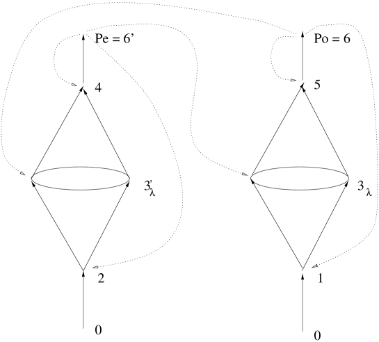
Figure 1: The lattices of submodules for the principal modules of $\cal H$

Since we have a totally explicit description of the algebra and of its lattice of representations, it is easy to continue the analysis and to investigate other properties of ${\cal H}$ illustrating many other general concepts from the study of non semi-simple associative algebras. One can, for instance, study the projective covers of the different representations (for completeness sake, this information is represented by dashed lines on figure 1), the subfactor representations, the quiver of the algebra, its Cartan matrix etc . This, however, would be a bit technical and more appropriate for a review paper (see [10]).

We want only to recall that there exists a one-to-one correspondence between irreducible representations of the algebra ${\cal H}$ and the principal modules $M_{st}$, $P_{e}$ and $P_{o}$. Irreducible representations are obtained from these principal modules by factorizing their radical, which amounts to kill the Grassmann “$\theta$” variables. From the above, we see that we obtain in this way three irreducible representations : a representation of dimension $3$, $M_{st}$ (it was already irreducible) which is a triplet for the unitary group $U(3)$ of the $M_{3}$ part of ${\cal H}$, a representation of dimension $2$, $S_{e}$ (the quotient of $P_{e}$ by its radical) which is a doublet for the unitary group $U(2)$ of the $M_{2|1}$ part of ${\cal H}$, and finally a representation of dimension $1$, $S_{o}$ (the quotient of $P_{o}$ by its radical), a $U(1)$ singlet. These are the three irreducible representations corresponding to the quotient $\overline{{\cal H}}$ of ${\cal H}$ by its Jacobson radical : (namely $\overline{{\cal H}}=\mbox{\rm C}\hskip-6.0pt\mbox{l}\;\oplus M_{2}(\mbox{\rm C}\hskip-6.0pt\mbox{l}\;)\oplus M_{3}(\mbox{\rm C}\hskip-6.0pt\mbox{l}\;)$).

The explicit definition given for ${\cal H}$ allows one to compute any tensor products of representations and reduce them. We have to consider the projective indecomposable representations ($P_{o}=\underline{6}$, $P_{e}=\underline{6^{\prime}}$ and $M_{st}=\underline{{3}}$) together with the irreducible ones ($S_{o}=\underline{1}$, $S_{e}=\underline{2}$ and $M_{st}=\underline{3}$). Here again appears a mixing between $M_{3}$ and $M_{2|1})$ via the coproduct, for instance, $\underline{6^{\prime}}\times\underline{2}\equiv\underline{6}+\underline{3}+\underline{3}$.

6 Others avatars for ${\cal H}$ and related algebras

In this paper, we decided to study properties of ${\cal H}$ without using any a priori knowledge on quantum groups. Here are nevertheless a few (non elementary) facts, given without proof, that may interest the reader.

Consider the universal enveloping algebra of $SL(2,\mbox{\rm C}\hskip-6.0pt\mbox{l}\;)$, say $U$. Let $U_{q}$ be the corresponding quantum algebra ($q=e^{h}$ is a deformation parameter) and $X_{\pm}$, $K$ its generators (not the same as before !).

• The first way to construct the finite dimensional Hopf algebra ${\cal H}$ from the infinite dimensional Hopf algebra $U_{q}$ is to divide it by an ideal (the ideal $I$ defined by the relations given in section $3$) and check that it is also a Hopf ideal (which means that $\Delta I\subset I\otimes{\cal H}+{\cal H}\otimes I$, $\epsilon(I)=0$ and $S(I)\subset I$).

  In the usual $U_{q}$ —more precisely in the so called adjoint rational form— and when $q$ is a cubic root of unity, the center is generated not only by the Casimir operator but also by the elements ${X_{\pm}}^{3}$ and $K^{3}$. It is therefore natural to define new algebras by dividing the ‘big’ object $U_{q}$ by an ideal generated by relations of the kind we just considered (remember that $K^{3}=1$ in ${\cal H}$). Actually, one could as well define new algebras by imposing relations of the kind $X_{\pm}^{\alpha}=0$ and $K^{\pm\gamma}=1$ for integers $\alpha$ and $\gamma$ that are divisible by $3$ (the value of the right hand side, namely $0$ or $1$ is fixed by the existence of a co-unit). The finite dimensional quotient ${\cal H}$ therefore appears as a “minimal” choice. As a matter of fact, even at the level of ${\cal H}$, defined as before, and without any reference to $U_{q}$, it is convenient to introduce an invertible square root $\hat{K}$ for $K$, hence $K={\hat{K}}^{2}$. In this way, one obtains a new algebra ${\cal H}^{tot}$ of dimension $2\times 27$ — just count the number of independent monomials $(X_{+}^{\alpha}{\hat{K}}^{\beta}X_{-}^{\gamma})$ when $X_{\pm}^{3}=0$ and ${\hat{K}}^{6}=1$ (this is a PBW basis). This algebra is quite interesting because its list of representations contains not only those of ${\cal H}$ but also “charge conjugate” representations. One can also justify, for the quantum enveloping algebra itself, and whether $q$ is a root of unity or not, the interest of adding a square root to the generator $K$. Introducing such a square root at the level of $U_{q}$ defines the the so-called simply-connected rational form of the quantum universal enveloping algebra. The reader should be warned that the algebra ${\cal H}$ or ${\cal H}^{tot}$ is sometimes denoted by $u_{q}(SL(2,\mbox{\rm C}\hskip-6.0pt\mbox{l}\;))$ —with a small $u$— and called the “restricted quantum universal algebra” (for a reason that will be explained below), but the terminology is not established yet and one should always look which of $K^{3}$ or $K^{6}$ is equal to $1$; for instance, our ${\hat{K}}$ —see above— coincide with the $K$ of [17].

• There exists another construction which is more tricky but maybe more profound. Let us start with the following simple observation. Consider the algebra of polynomials with one unknown $x$, over the rational numbers; it can be considered as an algebra generated by the $x^{i}$ (to be identified with the powers of $x$) with relations $x^{i}x^{j}=x^{i+j}$. One can make a change of generators, define the divided powers $x^{[i]}\doteq x^{i}/i!$ so that $x^{[i]}x^{[j]}={(i+j)!\over i!j!}x^{[i+j]}$ and define the very same algebra by using the new generators $x^{[i]}$ and the new relations. The tricky point is that, if we now decide to build an algebra over the finite field $F_{p}$ (for instance $\mbox{\rm Z}\hskip-4.0pt\mbox{\rm Z}/3\mbox{\rm Z}\hskip-4.0pt\mbox{\rm Z}$) by taking reduction of coefficients modulo $p$, the two constructions, with usual powers and divided powers, will lead to two different algebras. For instance, the relation $x^{1}x^{2}=x^{3}$ will be valid in the first algebra (the r.h.s. is non zero) whereas we obtain $x^{[1]}x^{[2]}={3!\over 1!2!}x^{[3]}=0$ if we use divided powers, since $3=0$ in $F_{3}$. A similar phenomenon appears, in the case of quantum groups when $q$ is a primitive root of unity. There are indeed two ways of specializing the $q$ of $U_{q}$ (see for instance [3]) to a particular complex value $\epsilon$. One can use the usual ($q$-deformed) generators and relations, but one can also use $q$-deformed divided powers and corresponding relations (these relations contain $q$-deformed factorials on the right hand side). For generic values of $q$, both definitions lead to the same algebra, but when $q$ is a primitive root of unity, the algebras are different. More precisely, we are interested here in the “restricted integral form”, called $U_{\epsilon}^{res}$ which is obtained as follows. We assume that $q=\epsilon$, with $\epsilon^{3}=1$, and start with $U_{\epsilon}$ considered as an algebra over the cyclotomic field $Q(\epsilon)$ (it is obtained by adjoining a cubic root of unity to the field $Q$ of rational numbers). $U_{\epsilon}^{res}$ is then defined as the subalgebra of $U_{\epsilon}$ generated by the elements $(X_{\pm})^{(r)}\doteq{(X_{\pm})^{r}\over[r]_{q}!}$, where $[r]_{q}!$ is the $q$ factorial — so these elements are $q$-deformed divided powers— and by $K^{\pm}$. Using $[n]_{q}!\doteq{(q^{n}-q^{-n})(q^{n-1}-q^{-(n-1)})\ldots(q-q^{-1})\over(q-q^{-1})^{n}}$, we see that $[1]!=1$, $[2]!=-1$ and $[N]_{q}!=0$ for $N>2$. This, in turn, implies that, in the algebra $U_{\epsilon}^{res}$, $(X_{\pm})^{3}=0$, $K^{3}$ is central and $K^{6}=1$. $U_{\epsilon}^{res}$ contains a finite dimensional Hopf subalgebra $U_{\epsilon}^{fin}$, of dimension $2\times 27$ over $Q(\epsilon)$, generated by $X_{\pm}$ and the $K^{s}$ for $s\in{0,1,\ldots,5}$. Since $K^{3}$ is central, one can also construct a quotient (of dimension $27$) by dividing $U_{\epsilon}^{fin}$ by the relation $K^{3}-1$. If we know take arbitrary complex coefficients (rather than coefficients belonging to $Q(\epsilon)$), we recover ${\cal H}$.

• Before ending this section, we want to comment about a rather beautiful and mysterious relation with Platonic bodies (actually with the simplest of them all, the tetrahedron). A finite Hopf algebra bearing some strong resemblance with ${\cal H}$ was originally defined by [12], [13] as the restricted enveloping algebra of a simple Lie algebra over the finite field $F_{p}$ with $p$ elements ($p$, a prime). The construction goes as follows :

  1. Start with an algebraic group $K$. In our case it will be $SL(2,F_{3})$. Note that this group, of order $24$ is isomorphic with the binary tetrahedral group (the double cover of the $SO(3)$ finite subgroup preserving a tetrahedron); the tetrahedron group itself is $PSL(2,F_{3})$ and is also isomorphic with the alternated group $A_{4}$.

  2. Construct $U_{Z}$, the so-called Chevalley-Kostant ZZ-form of the universal enveloping algebra $U$ for the corresponding Lie group $G$, in our case, $G=SL(2,\mbox{\rm C}\hskip-6.0pt\mbox{l}\;)$. It is a subring (over ZZ) of $U$ generated by the divided powers ${(X_{\pm})^{(r)}\over r!}$.

  3. Build the hyperalgebra of $SL(2,\mbox{\rm C}\hskip-6.0pt\mbox{l}\;)$ over $F_{p}$, namely $U_{F_{p}}\doteq U_{Z}\otimes_{\mbox{\rm Z}\hskip-4.0pt\mbox{\rm Z}}F_{p}$

  4. The restricted enveloping algebra $U_{F_{p}}^{fin}$ is the subalgebra of the hyperalgebra $U_{F_{p}}$ spanned by the $X_{\pm}$.

  The theory of restricted enveloping algebras $H_{q}=U_{F_{p}}^{fin}(G)$ goes back to [19] (see also his basic paper on derivations of algebras over a finite field [18]). $H_{p}$ is, in this way, defined for any Lie algebra ${\cal G}$ as a subring of the corresponding enveloping algebra generated by the divided powers of the Chevalley generators. The $p$-powers of these generators are zero and the obtained algebra is of dimension $p^{dim{\cal G}}$ over $F_{p}$. For us, ${\cal G}$ is $Lie(SL(2,C)$ and $F_{p}=F_{3}$ so that $dim\,H_{3}=27$. The purpose of defining objects like $H_{p}$ was historically to study the theory of modular representations of finite Chevalley groups. Although both $H_{p}$, defined as a restricted enveloping algebra over a finite field, and ${\cal H}$, defined as the quotient of $U_{\epsilon}^{fin}$ by the relation $(K^{3}-1)$ look like very different objects, (the first is an algebra over $F_{p}$, the second is over $Q(\epsilon)$ or over Cl ), it was shown by [20], [21] that there exists a natural bijection between representation theory over $F_{p}$ of the first and usual representation theory over Cl  of the second.

• Without entering this deep arithmetical discussion, we want to conclude this paragraph by a simple description of the theory of modular representations for the binary tetrahedral group $\Gamma\doteq\widetilde{Alt_{4}}=SL(2,F_{3})$. The table of usual (characteristic $0$) characters of $\Gamma$ is easy to obtain, for instance from the incidence matrix of the extended Dynkin diagram of $E_{6}^{(1)}$, via the McKay correspondence. The dimensions of irreducible representations are simply obtained by taking this diagram as a fusion diagram (tensorialization with the fundamental of dimension $2$). One obtains in this way the seven inequivalent irreducible representations of $SL(2,F_{3})$; see figure 2.

  

  Figure 2: Irreducible representations and fusion graph for the binary tetrahedral group

  Modular characters are only interesting in characteristic $2$ and $3$ (since primes $2$ and $3$ divide $24$). In characteristic $3$, there are only three regular conjugacy classes (namely the classes of the identity, minus the identity, and the class of the elements of period $4$). Therefore, using Brauer’s theory, one can check that there are also three irreducible inequivalent modular characters, of respective degrees $1$, $2$ and $3$ (like ${\cal H}$ !).

7 Other properties of ${\cal H}$

Differential algebras.

In order to build, in non commutative geometry, a generalized gauge theory model, or even something very elementary like the notion of generalized covariant differential, one needs the following three ingredients. 1) An associative algebra ${\cal A}$ (take for instance ${\cal A}={\cal H}$ or ${\cal A}={\cal H}\times C^{\infty}(R^{4}))$. 2) A module for ${\cal A}$ (choose any one you like). 3) A differential ZZ-graded algebra $(\Xi,d)$ that will replace the usual algebra of differential forms (De Rham complex). The choice of the last ingredient is not at all unique. For instance, one can take for $\Xi$:

1. The algebra $\Omega({\cal A})$ of universal differential form on ${\cal A}$ (one can always do so!). The differential algebra of universal forms on ${\cal H}$ is $\Omega({\cal H})=\bigoplus_{s=0}^{\infty}\Omega^{s}$ where $\Omega^{1}\subset{\cal H}\otimes{\cal H}$ is the kernel of the multiplication map, therefore, as a vector space, ${\cal H}={{\cal H}\otimes{\cal H}\over\Omega^{1}}$. Set $n=dim({\cal H})=p^{3}=27$, since $p=3$. We see that $\Omega^{1}$ is of rank $n-1$ as a ${\cal H}$-module and of complex dimension $dim\,\Omega^{1}=dim({\cal H})^{2}-dim({\cal H})=n(n-1)$. More generally, $\Omega^{s}=\Omega^{1}\otimes_{\cal H}\Omega^{1}\otimes_{\cal H}\ldots\otimes_{\cal H}\Omega^{1}$, so that $\Omega^{s}$ has rank $(n-1)^{s}$ as a ${\cal H}$ module and is of complex dimension $n(n-1)^{s}$.

2. The algebra $\Omega_{Der}({\cal A})$ of ${\cal A}$-valued antisymmetric forms on the Lie algebra of derivations of ${\cal A}$, which are linear w.r.t. the center of ${\cal A}$ ($Der{\cal A}$ is usually not an ${\cal A}$ module). This is the choice advocated by [15].

Understanding the structure of the Lie algebra $Der({\cal H})$ and of its own representation theory is an interesting subject which we plan to return to in a separate work. We just recall here a few basic facts. First of all derivations of $M_{n}(\mbox{\rm C}\hskip-6.0pt\mbox{l}\;)$ are all inner (they are given by commutators). The trace is therefore irrelevant and we can identify the Lie algebra of derivations of $M_{3}(\mbox{\rm C}\hskip-6.0pt\mbox{l}\;)$ with $Lie(SL(3,\mbox{\rm C}\hskip-6.0pt\mbox{l}\;))$. By imposing also a reality condition (hermiticity) one can obtain $Lie(SU(3))$. Suppose that one defines the algebra $M_{2}(\mbox{\rm C}\hskip-6.0pt\mbox{l}\;)\oplus\mbox{\rm C}\hskip-6.0pt\mbox{l}\;$ in terms of $3\times 3$ matrices as the linear span of elementary matrices $F_{11},F_{12},F_{21},F_{22}$ and $F_{33}$, it is easy to see that commutators with $F_{13},F_{23},F_{31}$ and $F_{32}$ define derivations that are not inner since these elements do not belong to $M_{2}(\mbox{\rm C}\hskip-6.0pt\mbox{l}\;)\oplus\mbox{\rm C}\hskip-6.0pt\mbox{l}\;$, but they are valued in the module of $3\times 3$ matrices. In a version of non commutative differential calculus using $\Omega_{Der}$, such derivations can be related to the notion of Higgs doublets. In the case of ${\cal H}$, which contains a Grassmann envelope (see first section), one has also to take into account the fact that the algebra is not semi-simple since it contains, in particular $(M_{2|1}(\mbox{\rm C}\hskip-6.0pt\mbox{l}\;)\otimes\Lambda^{2})_{0}$. Remember that derivations of Grassmann algebras are outer, and that, in particular, the vector space of graded derivations of a Grassmann algebra with two generators can be identified with the Lie superalgebra $Lie(SL(2|1))$ whose representation theory ([24]) is known to contain the representations that are needed to build the Standard Model of electroweak interactions (although the model is by no means obtained by gauging this superalgebra! See [26] and [8]).

3. When ${\cal A}$ is the tensor product of $\mbox{\rm C}\hskip-6.0pt\mbox{l}\;^{\infty}(M)$ by a finite dimensional algebra, one can also take $\Xi$ as the tensor product of the usual De Rham complex, for $M$, times the algebra of universal forms for the finite geometry. In the case of ${\cal A}=\mbox{\rm C}\hskip-6.0pt\mbox{l}\;^{\infty}(M)\otimes(\mbox{\rm C}\hskip-6.0pt\mbox{l}\;\oplus\mbox{\rm C}\hskip-6.0pt\mbox{l}\;)$ this was the choice made in [7] (see also [9]). Here, keeping in mind applications to particle physics, one could take for $\Xi$ the tensor product $\Lambda_{DR}\otimes\Omega({\cal H})$, where the first factor refers to the usual De Rham complex of differential forms over “space-time”.

4. The algebra $\Omega_{D}({\cal A})$ associated with a $K$-cycle on ${\cal A}$, i.e. the choice of a Hilbert space and a generalized Dirac operator $D$. This is the choice (“spectral triple”) advocated by [5] (and references therein).

In the present case, all of the above choices are possible, and also others, taking into account the existence of twisted derivations, etc . Since we do not plan here to build any particular physical model, we stop here our discussion concerning the choice of the differential algebra $(\Xi,d)$.

Powers of $SL(2)$ quantum matrices.

The following observation was made, in $1990$, by [31] and [11]: They show that the $n$-power of a quantum $SU(2)$ matrix with deforming parameter $q$ is a quantum matrix with deforming parameter $q^{n}$. This fact was then recovered and generalized in [22], [23] . We describe this as follows. Let $T\doteq\pmatrix{a&b\cr c&d}$ be a quantum $SL(2,\mbox{\rm C}\hskip-6.0pt\mbox{l}\;)$ matrix i.e., with $q$ an arbitrary complex number, we assume that symbols $a,b,c,d$ obey the six relations $ab=qba$, $bc=cb$, $ac=qca$, $bd=qdb$, $cd=qdc$ and ${\cal D}\doteq ad-qbc=da-q^{-1}bc$, a central element. We define then $a_{n},b_{n},c_{n},d_{n}$ by

$$\pmatrix{a_{n}&b_{n}\cr c_{n}&d_{n}}\doteq{\pmatrix{a&b\cr c&d}}^{n}$$

For instance $a_{2}=a^{2}+bc$, etc . One then shows that the six relations $a_{n}b_{n}=q^{n}b_{n}a_{n}$, etc , are satisfied. Actually, one proves that $T=q^{M}$, with $M\doteq\pmatrix{\lambda&\mu\cr\nu&-\lambda}$, where $\lambda,\mu$ et $\nu$ are operators obeying the relations $\left[\mu,\nu\right]=0$, $\left[\lambda,\mu\right]=\mu$ and $\left[\lambda,\nu\right]=\nu$. The result concerning powers of quantum matrices follows.

This result implies immediately that the “algebra of functions on $SL_{q^{r}}(2,\mbox{\rm C}\hskip-6.0pt\mbox{l}\;)$” is a subalgebra of the “algebra of functions on $SL_{q^{s}}(2,\mbox{\rm C}\hskip-6.0pt\mbox{l}\;)$” as soon as $s$ divides $r$ and that, in particular, the algebra of functions on the classical group $SL(2,\mbox{\rm C}\hskip-6.0pt\mbox{l}\;)$ is a subalgebra of ${Fun}\,SL_{q}(2,\mbox{\rm C}\hskip-6.0pt\mbox{l}\;)$ as soon as $q$ is a root of unity. This embedding, obtained by using properties of powers of quantum matrices is an embedding of algebra but not of coalgebras; this can be seen as follows (we compare ${Fun}\,SL_{q}(2,\mbox{\rm C}\hskip-6.0pt\mbox{l}\;)$ and ${Fun}\,SL_{q^{2}}(2,\mbox{\rm C}\hskip-6.0pt\mbox{l}\;)$): the coproduct on the algebra spanned by the coordinate functions $\langle a,b,c,d\rangle$ generating ${\mathsl Fun}(SL_{q}(2,\mbox{\rm C}\hskip-6.0pt\mbox{l}\;))$ reads, when applied to the generator $a$, $\Delta a=a\otimes a+b\otimes c$, etc . Since $\Delta$ is an algebra homomorphism $\Delta a_{2}=\Delta a^{2}+\Delta(bc)=\Delta a\Delta a+\Delta b\Delta c$ i.e. $\Delta a_{2}=(a\otimes a+b\otimes c)(a\otimes a+b\otimes c)+(a\otimes b+b\otimes d)(c\otimes a+d\otimes c)=a^{2}\otimes a^{2}+ba\otimes ca+ab\otimes ac+b^{2}\otimes c^{2}+ac\otimes ba+ad\otimes bc+bc\otimes da+b^{2}\otimes dc$, whereas the Hopf algebra ${\mathsl Fun}(SL_{q^{2}}(2,\mbox{\rm C}\hskip-6.0pt\mbox{l}\;))$ has another coproduct, namely $\Delta^{\prime}a_{2}=a_{2}\otimes a_{2}+b_{2}\otimes c_{2}$ equal to $\Delta^{\prime}a_{2}=(a^{2}+bc)\otimes(a^{2}+bc)+(ab+bd)\otimes(ca+dc)$. Therefore $\Delta$ and $\Delta^{\prime}$ are usually different.

Warning: We already mentioned the fact that ${\cal H}_{q}^{tot}$ (more precisely $U_{\epsilon}^{fin}$) can be considered as a Hopf subalgebra of $U_{q}(SL(2,\mbox{\rm C}\hskip-6.0pt\mbox{l}\;))$ provided we define it by using divided powers of the Chevalley generators. We do not know any relation between this kind of embedding, which can be generalized to other $q$-analogues of Lie simple groups [20] and [21]) and the algebra embedding mentioned above (which seems to be only valid for $SL_{q}(2)$).

General remarks.

Embedding of ${Fun}\,SL(2,\mbox{\rm C}\hskip-6.0pt\mbox{l}\;)$ in ${Fun}\,SL_{q}(2,\mbox{\rm C}\hskip-6.0pt\mbox{l}\;)$ (with $q$ a root of unity) can be visualized as a projection from the quantum group to the classical one, with a finite quantum group as “fiber”. This finite quantum group should therefore itself be thought of as a “group” included in $SL_{q}(2,\mbox{\rm C}\hskip-6.0pt\mbox{l}\;)$. Despite of the free use of a terminology borrowed from commutative geometry, note that in the present situation, spaces have no points (or very few…)! Morally, one would like to replace the enveloping algebra of the Lorentz group $Spin(3,1)=SL(2,\mbox{\rm C}\hskip-6.0pt\mbox{l}\;)$ by the quantum enveloping algebra of $SL_{q}(2,\mbox{\rm C}\hskip-6.0pt\mbox{l}\;)$, when $q^{3}=1$. At the intuitive level (and although theses spaces have very few points) one can see the classical Lorentz group as a quotient of the quantum $SL_{q}(2,\mbox{\rm C}\hskip-6.0pt\mbox{l}\;)$, with $q$ a primitive root of unity, by a “discrete quantum group” described by ${\cal H}$. This was the idea advocated in a comment of [4]. We refrain to insist on the obvious similarities between some aspects of representation theory of ${\mathcal{H}}$ and the Standard Model of elementary particles. We also refrain to insist on the obvious differences$\ldots$ Notice that the finite quantum group ${\cal H}$, of dimension $27$ (or ${\cal H}_{tot}$, of dimension $2\times 27$) is an analogue of the discrete group $\mbox{\rm Z}\hskip-4.0pt\mbox{\rm Z}_{2}$ that describes the relation between the Lorentz group and the spin group (the latter being the universal cover of the former): $SO(3,1)=Spin(3,1)/\mbox{\rm Z}\hskip-4.0pt\mbox{\rm Z}_{2}$, relation which is, classically, at the origin of the difference between particles of integer and half-integer spin. Here, we have something analogous for ${\cal H}$. Whether or not one can build a realistic physical model along these lines, with non trivial prediction power, remains to be seen. We hope that the present contribution may help the interested readers to develop new ideas in this direction.

Acknowledgments

Many results to be found here came from discussions with Oleg Ogievetsky. I want to thank him for many enlightening comments and, in particular, for his patience in explaining me the basics concerning representation theory of non semi-simple associative algebras.

This work was supported, in part, by a grant from the Instituto Balseiro (Centro Atomico de Bariloche). I want to thank everybody there for their warm hospitality and for providing a peaceful atmosphere which made possible the writing of these notes.

References

• [1] A. Alekseev, D. Gluschenkov and A. Lyakhovskaya, Regular representation of the quantum group $SL_{q}(2)$ ($q$ is a root of unity), St. Petersburg Math. J., Vol 6, N5, p 88-114 (1994)
• [2] D. Arnaudon, Fusion Rules and ${R}$-matrices for representations of $SL(2)_{q}$ at roots of unity, hep-th/9203011
• [3] V.Chari, A.Pressley, A guide to Quantum Groups, Cambridge University Press (1994)
• [4] A. Connes NonCommutative Geometry and Reality, IHES/M/95/52
• [5] A. Connes, Gravity coupled with matter and foundation of non-commutative geometry, hep-th/9603053
• [6] A. Connes and A. Chamseddine, The spectral action principle, hep-th 9606001
• [7] R. Coquereaux, G. Esposito-Farese and G. Vaillant, Higgs fields as Yang-Mills fields and discrete symmetries, Nucl. Phys. B353, 689 (1991).
• [8] R. Coquereaux, G. Esposito-Farese and F. Scheck, An $SU(2|1)$ theory of electroweak interactions described by algebraic superconnections, Int. Jour. of Mod. Phys. A, Vol. 7, No 26 (1992) 6555-6593
• [9] R. Coquereaux, R. Haussling and F. Scheck, Algebraic connections on parallel universes, Int. Jour. of Mod. Phys. A, Vol. 10, No 1 (1995) 89-98
• [10] R. Coquereaux, O. Ogievetsky. Comments on the properties of finite dimensional Hopf algebras related with $SL_{q}(2)$ when $q$ is a primitive root of unity, CPT-Preprint. To appear.
• [11] E. Corrigan, D. Fairlie, P. Fletcher and R. Sasaki, Some aspects of quantum groups and supergroups, J. Math. Phys. 31, 776 (1990)
• [12] C.W. Curtis, Modular Lie Algebras. I, Transac. of the Amer. Math. Soc., Vol 82 p 161-179 (1956)
• [13] C.W. Curtis, Representation of Lie algebras of classical type with applications to linear groups, J. Math. Mech. 9, 307-326 (1960)
• [14] P. Di Francesco and J.-B. Zuber, in Recent Developments in Conformal Field Theories, Trieste Conference, 1989, S. Randjbar-Daemi, E. Sezgin and J.-B. Zuber eds., World Scientific 1990
• [15] M. Dubois Violette, Derivations et calcul differentiel non commutatif, C.R.A.S. Paris, 307, SΓ©rie I (1988), 403-408
• [16] M. Dubois Violette Non-commutative differential geometry, quantum mechanics and gauge theory, in Differential Geometric Methods in Theoretical Physics, Rapallo 1990 (C. Bartocci, U. Bruzzo,, R. Cianci, eds), Lecture Notes in Physics 375, Springer-Verlag 1991.
• [17] D.V. Gluschenkov, A.V. Lyakhovskaya, Regular representation of the quantum Heisenberg double ($q$ is a root of unity), Zapiski LOMI 215 (1994).
• [18] N. Jacobson, Abstract Derivation and Lie algebra, Transac. of the Amer. Math. Soc., Vol 42 p 206-224 (1937)
• [19] N. Jacobson, Restricted Lie algebras of characteristic p, Transac. of the Amer. Math. Soc., Vol 50 p 15-26 (1941)
• [20] G. Lusztig, Finite dimensional Hopf algebras arising from quantized universal enveloping algebras, J. of the Amer. Math. Soc., Vol 3, N1, p 257-296 (1990)
• [21] G. Lusztig, Quantum groups at roots of $1$, Geometrica Dedicata,Vol 35, p 89-114 (1990)
• [22] H.Ewen, O. Ogievetsky and J. Wess, Quantum matrices in two dimensions, Letters in Math. Phys. 22, 297-305, 1991
• [23] O. Ogievetsky and J. Wess Relations between $GL_{(p,q)}(2)$’s, Z. Phys. C - Particles and Fields 50,123,131 (1991)
• [24] M. Marcu, The representations of $spl(2|1)$, J.Math. Phys. 21(6) 1277-1283 (1980)
• [25] C.P. Martin, J. Gracia Bondia and J. Varilly, The Standard Model as a noncommutative geometry: the low mass regime, hep-th/9605001
• [26] Y. Ne’eman, J. Thierry-Mieg, Anomaly-free sequential superunification, Phys. Lett. B108 (1982) 399-402
• [27] A. Ocneanu, private communication. See also: Paths on Coxeter diagrams, from Platonic solids and singularities to minimal models and subfactors (notes recorded by S. Goto, Univ. of Tokyo (in Japanese))
• [28] O. Ogievetsky, Matrix structure of $SL_{q}(2)$ when $q$ is a root of unity. CPT-96/P3390
• [29] V. Pasquier and H. Saleur, Common structure between finite systems and conformal field theories through quantum groups, Nucl. Phys. B330 (1990) 523
• [30] R. Suter, Modules over ${\mathsl U}_{q}(SL2)$, Comm. in Math. Phys., Vol 163, p 359-393 (1994)
• [31] S. Vokos, J. Wess and B. Zumino, Analysis of the basic matrix representation of $GL_{q}(2,\mbox{\rm C}\hskip-6.0pt\mbox{l}\;)$, Z. Phys. C48, 65 (1990)