Magnetic monopole loop for the Yang-Mills instanton

Abstract

We investigate ’t Hooft-Mandelstam monopoles in QCD in the presence of a single classical instanton configuration. The solution to the Maximal Abelian projection is found to be a circular monopole trajectory with radius $R$ centered on the instanton. At zero loop radius, there is a marginally stable (or flat) direction for loop formation to $O(R^{4}logR)$. We argue that loops will form, in the semi-classical limit, due to small perturbations such as the dipole interaction between instanton anti-instanton pairs. As the instanton gas becomes a liquid, the percolation of the monopole loops may therefore provide a semi-classical precursor to the confinement mechanism.

I Introduction

Both instantons and magnetic monopoles are thought to play an important role in the Euclidean description of the Yang-Mills vacuum. In QCD instantons provide the solution to the $U(1)$ problem [1] and a vacuum composed of a liquid of instantons [2] can explain chiral symmetry breaking and the low mass spectrum, at least at a qualitative level [3, 4]. Nonetheless, it is generally believed, as conjectured by Mandelstam [5] and ’t Hooft [6], that magnetic monopoles, not instantons are essential for confinement in QCD and related gauge theories. For example, compact QED with a lattice cutoff is known to be exactly dual to a Coulomb gas of monopoles, which upon condensation causes confinement via a dual Meisner effect [7]. Similarly there is evidence for the role of monopole condensation in the 3-d Yang-Mills-Higgs (or Georgi-Glashow) model [8] and more recently in 4-d N = 2 supersymmetric Yang-Mills theory [9].

Consequently, we are faced with a dilemma of two competing pictures of the QCD vacuum (or more accurately the Euclidean equilibrium phase) as either a coherent ensemble of instantons or a condensate of magnetic monopoles. In this paper, we show that these two pictures may in fact be two descriptions for the same phase. To establish a precise and indisputable link between the monopole trajectories and instantons, we define the monopole current in a field configuration via ’t Hooft’s Maximal Abelian (MA) projection and demonstrate that in the background of a single instanton the MA projection leads to a circular monopole current loop of radius $R$ centered on an isolated instanton of “width” $\rho$. We also begin the study of monopole trajectories in the presence of interacting instanton pairs.

Let us review briefly the attempts to identify monopole currents in QCD. (The reader is referred to Polikarpov [10] and references therein for more details.) It is well known that the only topological stable solutions to Euclidean Yang-Mills theory are the multi-instanton solutions [11] with topological charge $Q$. On the other hand, the ’t Hooft-Polyakov monopole solution to 3-d Yang-Mills-Higgs theory can also be viewed as a static solution to the pure Yang-Mills Euclidean field equations in 4-d, where $A_{0}$ plays exactly the same role as the adjoint Higgs field in the BPS limit. Of course, since the classical theory is now scale invariant the monopole mass M is an arbitrary parameter. Quantum effects will be necessary to set the scale. Subsequently Rossi [13] has pointed out that this monopole configuration can be identified with (i.e., has the same field configuration as) an infinite sequence of instantons equally spaced by $M^{-1}8\pi^{2}/e^{2}$ on the time axis in the limit $\rho\rightarrow\infty$.

Turning now to the MA projection, Chernodub and Gubarev [14] have recently shown that a straight line monopole trajectory through the center of an instanton (or pair of instantons) satisfied the MA gauge condition. However if one looks at the MA gauge fixing functional, $G={\textstyle{1\over 4}}\int d^{4}xA^{+}_{\mu}(x)A^{-}_{\mu}(x)$, $A^{\pm}_{\mu}\equiv A^{1}_{\mu}\pm iA^{2}_{\mu}$, for the Chernodub-Gubarev solution, one notices that it diverges at large distances. Since the proper definition of the MA projection is not just a stationary point but a minimum of this functional, this solution is still not a very satisfactory linkage between an instanton and the monopole. The basic problem is that the instanton is restricted to a space-time region whereas the static monopole solution has an infinite trajectory. In contrast we have found that our monopole loop solution to the MA projection, which is localized at the instanton, does give a finite value to $G$, which drops gradually to an absolute minimum as the radius decreases: $G\simeq 4\pi^{2}\rho^{2}[1+4.6(R/\rho)^{4}log(\rho/R)]$. We then argue that this solution is easily stabilized by small Gaussian perturbations or nearby interactions with anti-instantons. We feel this is the first rather precise connection between the instanton and monopole trajectories.

In addition to this continuum analysis, there has been some recent numerical evidence in lattice simulations presented by Hart and Teper [15], by Bornyakov and Schierholz [16], and by Markum et al. and Thurner et al. [17] that shows that monopole loops are correlated with multi-instantons configurations. These numerical results also indicate that a correlation between monopole condensation and the formation of a dense liquid of instantons are a property of the quantum vacuum. However our immediate goal is a more modest one: establishing a clear kinematical connection between monopoles and instantons in the semi-classical limit. While this limited exercise is unable to show that the dynamics of the full quantum theory is in some sense approximated by a monopole-instanton correlated background and that confinement results from the percolation of these objects, we feel that clarifying the kinematics is an important first step in bringing these two pictures together.

To go beyond the analytical study, we have also undertaken a numerical MA projection in the background of an isolated instanton by minimizing the functional $G$ discretized on a 4-d hypercubic lattice. The only solutions we have found were identical to our analytical monopole loop solution albeit stabilized to a fixed radius (in lattice units) by lattice artifacts. We have also begun to study the monopole loops in the background of an interacting instanton anti-instanton (I-A) pair and found that the individual loops appear to be stabilized by the interaction, if the I-A molecule is oriented so that the dipole interaction is attractive. At a critical separation of the I-A pair, the individual monopole loops fuse into a single loop. Details of the multi-instanton study are left to a future publication [18]. Nonetheless on the basis of our preliminary analysis, we conjecture that the I-A interaction provides a semi-classical mechanism whereby the monopoles are “liberated” from the individual instantons, and which may therefore represent a precursor to condensation and confinement.

The organization of the paper is as follows. We begin by noting that the Maximal Abelian projection, which is usually presented as a gauge fixing procedure is equivalent to the introduction of an “auxiliary Higgs” field $\Phi=\vec{\phi}\cdot\vec{\tau}$, which is determined by minimizing the Higgs kinetic term,

$$G={{\textstyle{1\over 4}}}\int d^{4}x[D_{\mu}(A)\vec{\phi}]^{2},$$ (1)

(The Higgs field is related to the usual gauge rotation by $\Phi=\Omega^{\dagger}\tau_{3}\Omega$.) This approach has several advantages in terms of analysis and a clearer relation to the standard discussion of monopole topology. (See Appendix A for details.)

Next in Section 2, we solve the stationarity equations for the Higgs field (or gauge rotation in the $SU(2)/U(1)$ coset space), to find the monopole loop solution for fixed radius $R$. Monopole loops in Abelian gauge theories are reviewed to guide the construction.

In Section 3, we consider the full manifold of solutions and their collective co-ordinates. We note that there is an interesting correlation between the average over the orientations of all monopole loops at fixed $R$ and the isospin orientation of the instanton given by

$$<N_{\mu\nu}>={\textstyle{1\over 2}}[(\delta_{\mu,3}\delta_{\nu,4}-\delta_{\mu,3}\delta_{\nu,4})-(\delta_{\mu,1}\delta_{\nu,2}-\delta_{\mu,2}\delta_{\nu,1})]$$ (2)

where $N_{\mu\nu}$ is the skew symmetric unit tensor defining the plane of the loop in 4-d.

In Section 4, we report on our numerical solutions leading to a preliminary picture of the role of instanton anti-instanton (I-A) interactions for loop stabilization at large separation and for the I-A pair loop fusion and percolation at small separations.

Finally in Section 5, we discuss our results and suggest future lines of investigation. We comment on the naturalness of the instanton-monopole connection. The loop “VEV” naturally breaks the $SO(4)$ group down to the coset direct product $SU_{L}(2)/U_{L}(1)\times SU_{R}(2)/U_{R}(1)$ in close analogy to isospin breaking in the ’t Hooft-Polyakov monopole construction. Also we note that the Abelian projection for the instanton in the singular gauge spreads the singularity at the origin to the trajectory of the monopole loop, directly relating the instanton’s topological charge $Q$ to the monopole charge $g$ by the identity $Q=eg/4\pi$. In summary we conclude that monopole loops are peculiarly well matched to the instanton, leading us to hope that there is a deeper connection in confining gauge theories transcending our particular construction.

II Monopole Loop Solution in the Instanton Background

The Maximal Abelian projection was introduced by ’t Hooft [6] in order to define magnetic monopole coordinates by a partial gauge fixing procedure that leaves the maximal Abelian subgroup free. In analogy with the Higgs system, ’t Hooft suggested introducing an adjoint field $X$, which by the gauge transformation, $X\rightarrow X^{\Omega}=\Omega X\Omega^{\dagger}$, is diagonalized to fix the gauge in the coset space $SU(N)/U(1)^{N-1}$ up to $U(1)$ factors. Exceptional space-time trajectories where $X$ has degenerate eigenvalues represent the Abelian monopole configurations. Various examples for X were suggested such as $F_{12}$ or the (untraced) Polyakov loop, etc.

Subsequently a particular Lorentz covariant gauge has proven to best correlate the monopoles condensate with confinement in lattice simulations [19]. This gauge is now referred to as the Maximal Abelian (MA) gauge. For $SU(2)$, it is expressed as the minimization of the functional,

$$G[A_{\mu}]={\textstyle{1\over 4}}\int d^{4}xA^{+}_{\mu}(x)A^{-}_{\mu}(x)\;,$$ (3)

$A^{\pm}_{\mu}\equiv A^{1}_{\mu}\pm iA^{2}_{\mu}$. In differential form the MA gauge condition becomes

$$\Delta^{\pm}(x)\equiv(\partial_{\mu}\pm ieA^{3}_{\mu})A^{\pm}_{\mu}=0\;,$$ (4)

with the additional stipulation to avoid Gribov copies that one should find the solutions corresponding to the global minimum of $G$. (We will sometime refer to the stationarity condition (4) by itself as the “differential” MA projection.)

Before presenting the details of our monopole loop solution, it is possible (at least with hindsight) to see why magnetic loops might appear in an instanton background. Consider the field configuration for a single instanton [20, 21, 22] in the singular gauge,

$$A_{\mu}\equiv{\textstyle{1\over 2}}\vec{A}_{\mu}\cdot\vec{\tau}={\textstyle{{e}\over{2}}}\tau^{a}\bar{\eta}^{a}_{\mu\nu}\partial_{\nu}ln(1+\rho^{2}/x^{2}),$$ (5)

where the anti-self-dual ’t Hooft symbol is $\bar{\eta}^{a}_{\mu\nu}\equiv(i/2)Tr(\tau^{a}\tau_{\nu}\tau_{\mu}^{\dagger})$ and $\tau_{\mu}=(i,\vec{\tau})$ with Latin indices restricted to the vector components. First one notices that this field configuration already satisfies the differential MA (as well as the Lorentz) gauge condition. Also it gives a finite value,

$$G[A_{\mu}]=2e^{2}\int d^{4}x\frac{\rho^{4}}{x^{2}(x^{2}+\rho^{2})^{2}}=4\pi^{2}e^{2}\rho^{2},$$ (6)

to the MA gauge fixing functional — the dominant contribution to $G$ coming from the core of the instanton, $0\leq x\leq\rho$. On the other hand, the instanton in the non-singular gauge also satisfies the differential Eq. (4) for the MA projection, but now the functional $G$ diverges logarithmically at large distances,

$$G[A^{(ns)}_{\mu}]=2e^{2}\int d^{4}x\frac{\rho^{2}}{(x^{2}+\rho^{2})^{2}}\rightarrow\infty.$$ (7)

Nonetheless, the non-singular gauge does reduce the contribution to $G$ in the core of the instanton. Consequently, comparison between the singular and non-singular gauges suggests that it might be possible to find an intermediate solution which minimizes $G$ by a gauge transformation such that the central region, inside some radius ($x\leq R$), is converted to the non-singular gauge, while the large distance behavior is unchanged from the singular gauge configuration. In essence this will turn out to be the way we construct the monopole loop solution.

In addition, by a general argument one can understand why this construction might lead to monopole singularities. No local gauge transformation on the instanton can change the total topological charge. However if we express the topological charge for the instanton in the singular gauge via Gauss’ law, $Q=\int d^{4}x\partial_{\mu}K_{\mu}$, in terms of the flux for the gauge variant current,

$$K_{\mu}=\frac{1}{8\pi^{2}}\epsilon_{\mu\nu\rho\lambda}Tr[A_{\nu}(\partial_{\rho}A_{\lambda}-{\textstyle{{2i}\over{3}}}A_{\rho}A_{\lambda})]\;,$$

one knows that the entire contribution comes from the singular point at $x=0$. Any gauge rotation that removes this singularity but does not change the gauge at infinity must replace it with another singularity at some finite distance. As we will explain in more detail in the conclusion, our monopole loop current is the source of this singularity and its magnetic charge can therefore be directly related to the topological charge of the instanton.

A General Equations

In searching for solutions to the MA projection, we have found it more convenient to use a gauge covariant formulation in terms of an auxiliary Higgs-like field, $\Phi(x)\equiv\Omega^{\dagger}\tau_{3}\Omega$, instead of working directly with the gauge transformation $\Omega(x)$ itself (see Appendix for details). In terms of the isovector field $\vec{\phi}$, $\Phi\equiv\vec{\phi}\cdot\vec{\tau}$, the functional $G$ becomes

$$G={\textstyle{1\over 2}}\int d^{4}x\{{\textstyle{1\over 2}}[D_{\mu}(A)\vec{\phi}]^{2}+V(\vec{\phi}^{2})\},$$ (8)

where $D_{\mu}\phi^{\alpha}\equiv\partial_{\mu}\phi^{\alpha}+e\epsilon^{\alpha\beta\gamma}A_{\mu}^{\beta}\phi^{\gamma}$ and the potential is $V(\vec{\phi}^{2})=\sigma(\vec{\phi}^{2}-1)$ with a Lagrange multiplier $\sigma$. (One can see by inspection that Eq. (8) is identical to Eq. (3), after the substitution $\Phi\equiv\Omega^{\dagger}\tau_{3}\Omega$.) It is also natural to generalize the MA projection with a quartic Higgs potential,

$$V(\vec{\phi}^{2})={\textstyle{1\over 4}}\lambda(\vec{\phi}^{2}-v^{2})^{2},$$ (9)

with $\Phi(x)$ now given by $\vec{\phi}(x)\cdot\vec{\tau}/|\vec{\phi}(x)|$. We will refer to this more general from as the “Higgs MA projection”. The conventional MA projection is recovered in the limit $\lambda\rightarrow\infty$ at fixed VEV $v$ in which the Higgs mass scale $m_{H}\rightarrow\infty$ as well. Not only does the covariant formulation have numerous technical advantages, it shows that the MA projection need not be seen as a gauge fixing prescription but instead as a gauge covariant method of identifying the appropriate magnetic variables.

The general problem is to construct solutions to the differential form of the MA projection,

$$D_{\mu}(A)^{2}\vec{\phi}-\vec{\nabla}_{\phi}V(\phi)=0\;,$$ (10)

in the background of a single instanton. For the standard MA projection, this yields a linear PDE for $\vec{\phi}(x)$,

$$\partial_{\mu}^{2}\vec{\phi}+2\vec{A}_{\mu}\times\partial_{\mu}\vec{\phi}+\vec{A}_{\mu}\times(\vec{A}_{\mu}\times\vec{\phi})-\sigma\vec{\phi}=0,$$ (11)

subject to the constraint $\vec{\phi}^{2}=1$. For an instanton in the singular gauge (5), the potential also can be written as $A_{\mu}=-ix^{2}f(x)g^{\dagger}(x)\partial_{\mu}g(x)$, where $g^{\dagger}(x)=-ix_{\mu}\tau_{\mu}/|x|$, $\tau_{\mu}=(\vec{\tau},i)$,

$$f(x)=\frac{1}{x^{2}}\frac{\rho^{2}}{x^{2}+\rho^{2}},$$ (12)

and we have also set the gauge coupling $e=1$.

Solving this equation is very similar to the problem, first considered by ’t Hooft [1], for computing the Gaussian fluctuations of gauge, fermionic and Higgs fields in the background of an instanton. In studying self-dual solutions and their supersymmetric extensions, it is useful to introduce tensors that reflect the chiral $SU_{L}(2)\times SU_{R}(2)$ decomposition of the $O(4)$ Euclidean Lorentz group, which suggests the conformal coordinates, ${\tt u}=x+iy=ue^{\textstyle{i\varphi}}$ and ${\tt v}=z+it=ve^{\textstyle{i\psi}}$, that enter into the bispinor,

$$x_{\alpha\dot{\beta}}\equiv x_{\mu}(\tau_{\mu})_{\alpha\dot{\beta}}=\pmatrix{z+it&x-iy\cr x+iy&-z+it\cr}=\pmatrix{{\tt v}&{\tt u}^{*}\cr{\tt u}&-{\tt v}^{*}\cr}$$ (13)

for the singular gauge transformation, $g^{\dagger}(x)_{\alpha\dot{\beta}}=-ix_{\alpha\dot{\beta}}/|x|$. This notation, as we will see in Sec. 3, is also convenient for exhibiting the Lorentz symmetries of the monopole solution.

It follows from the property of $\bar{\eta}^{\alpha}_{\mu\nu}$ that isospin components of $\vec{A}_{\mu}$ are orthogonal, i.e., $A_{\mu}^{\alpha}A_{\mu}^{\beta}\propto\delta_{\alpha\beta}$. As a consequence, the last two terms in Eq. (11) both point along $\vec{\phi}$ in the isospin space. Let us parameterize this “radial direction” at each $x$ by a unit-vector,

$$\hat{\phi}(x)\equiv(\sin\beta\cos\alpha,\sin\beta\sin\alpha,\cos\beta)$$ (14)

and introduce two unit tangent-vectors orthogonal to $\hat{\phi}(x)$, $\hat{\alpha}(x)\equiv(-\sin\alpha,\cos\alpha,0)$ and $\hat{\beta}(x)$ $\equiv(\cos\beta\cos\alpha,\cos\beta\sin\alpha,-\sin\beta)$. By projecting Eq. (11) onto the $\hat{\alpha}(x)$ and $\hat{\beta}(x)$ axes, the two independent differential equations for the MA gauge are

$$\sin\beta\;\partial^{2}_{\mu}\alpha+2\cos\beta\;(\partial_{\mu}\alpha)(\partial_{\mu}\beta)=-2\sin\beta(\hat{\phi}\cdot\vec{A}_{\mu})\;(\partial_{\mu}\beta),$$ (15)

$$\partial^{2}_{\mu}\beta-{\textstyle{1\over 2}}\sin(2\beta)\;(\partial_{\mu}\alpha)^{2}=2\sin\beta(\hat{\phi}\cdot\vec{A}_{\mu})\;(\partial_{\mu}\alpha),$$ (16)

respectively. (The more general equations for the Higgs MA projection for arbitrary $\lambda$ are given in Eqs. (A15 - A17).) Our task is to find solutions to these equations.

For the explicit monopole content of a solution, it is instructive to return to the active transformation, Eq. (A1), and to decompose the transformed field into two parts, Eq. (A2), $A^{\Omega}_{\mu}(x)=\bar{A}_{\mu}(x)\;+\;M_{\mu}(x)\;$ where

$$\bar{A}_{\mu}(x)\equiv\Omega(x)A_{\mu}(x)\Omega^{\dagger}(x)\;\;,\;\;M_{\mu}(x)\equiv\frac{1}{ie}\Omega(x)\partial_{\mu}\Omega^{\dagger}(x)\;.$$

The gauge rotation in terms of three Euler’s angles is

$$\Omega(x)=e^{\textstyle{i\omega(x)}}=e^{\textstyle{i\gamma\tau_{3}/2}}e^{\textstyle{i\beta\tau_{2}/2}}e^{\textstyle{i\alpha\tau_{3}/2}}.$$ (17)

One can readily verify that this is consistent with Eq. (14) and, owing to the residual $U(1)$ invariance, $\vec{\phi}(x)$ is independent of the angle $\gamma$. Focusing on the Abelian field $a_{\mu}(x)\equiv Tr(\tau_{3}A_{\mu}^{\Omega})=\bar{A}_{\mu}^{3}+M_{\mu}^{3}$, one observes that the first term $\bar{A}_{\mu}^{3}=\hat{\phi}\cdot\vec{A}_{\mu}$ provides the source for our PDE’s, Eqs. (15) and (16). The induced term,

$$M_{\mu}^{3}(x)=-\frac{1}{e}[\cos\beta(x)\partial_{\mu}\alpha(x)+\partial_{\mu}\gamma(x)],$$ (18)

will give rise to topological current for the monopoles, Eq. (A5). In terms of the Euler’s angles, the magnetic current is explicitly given as,

$$k_{\mu}(x)=\frac{1}{2\pi e}\epsilon_{\mu\nu\rho\sigma}\partial_{\nu}[\partial_{\sigma}\alpha(x)\partial_{\rho}\cos\beta(x)].$$ (19)

Note that $M^{3}_{\mu}$ is not specified uniquely due to the residual $U(1)$ gauge symmetry. Generally, we will choose $\gamma(x)=-\alpha(x)$ so that the Dirac sheet associated with the monopole loop solutions can be oriented conveniently and so that

$$\Omega(x)=\cos(\beta/2)+i\sin(\beta/2)[(\cos\alpha)\tau_{1}-(\sin\alpha)\tau_{2}]$$ (20)

obeys the boundary condition $\Omega\rightarrow 1$ as $\beta\rightarrow 0$.

B Monopole Loop in $U(1)$ Gauge Theory

To construct monopole loop solutions, we have found it helpful to work “backward” from specific examples of $U(1)$ monopole currents. First, recall Dirac’s construction for a static monopole of magnetic charge $g$ at the origin $x=y=z=0$, with magnetic current, $k_{\mu}(x)=g\delta^{(3)}(\vec{x})\delta_{\mu 4}$. The field is given by

$$a_{\mu}=\frac{g}{4\pi}[1-\cos\vartheta]\partial_{\mu}\varphi,$$ (21)

in spherical coordinates, $0\leq\vartheta\equiv\tan^{-1}(\sqrt{x^{2}+y^{2}}/z)\leq\pi$ and $\varphi=\tan^{-1}(y/x)$. The singular behavior due to $\partial_{\mu}\varphi=\hat{\varphi}/\sqrt{x^{2}+y^{2}}$ as $\sqrt{x^{2}+y^{2}}\rightarrow 0$ corresponds to having placed a Dirac string along the negative $z$-axis, which in 4-d leads to a Dirac sheet in the left-half of the 3-4 plane. The Dirac sheet can be moved by a gauge transformation.

This construction is an example of a general formalism for writing down a solution with a Dirac sheet attached to a closed Euclidean monopole current loop [23]. Consider a unit monopole trajectory $x_{\mu}=y_{\mu}(\tau)$ and its associated magnetic current $k_{\mu}(x)=\int d\tau\partial_{\tau}y_{\mu}(\tau)\delta^{4}(x-y)$. We can attach to it a Dirac sheet described by $y_{\mu}(\tau,\sigma)$, where $x_{\mu}=y_{\mu}(\tau,0)$. The associated vector potential for the monopole loop is

$$a_{\mu}(x)=-\frac{1}{4\pi}\int d^{4}x^{\prime}\frac{\partial_{\nu}\tilde{G}_{\nu\mu}(x^{\prime})}{|x-x^{\prime}|^{2}},$$ (22)

where $\tilde{G}_{\mu\nu}={\textstyle{1\over 2}}\epsilon_{\mu\nu\rho\sigma}G_{\rho\sigma}$ and $G_{\mu\nu}(x)=\int d\tau d\sigma\{\partial_{\tau}y_{\mu}\partial_{\sigma}y_{\nu}-\partial_{\tau}y_{\nu}\partial_{\sigma}y_{\mu}\}\delta^{4}(x-y(\tau,\sigma))$.

We now apply Eq. (22) to a monopole of charge $g$ moving in a closed loop of radius $R$ in the 3-4 plane centered at the origin. The Dirac sheet (or solenoid world sheet) is chosen to run across the loop (see Fig 1), parameterized by $y_{1}=y_{2}=0$, $y_{3}=R(1-\sigma)\cos\pi\tau$, $y_{4}=R(1-\sigma)\sin\pi\tau$, where $-1\leq\tau<1$, and $0\leq\sigma<1$. It is convenient to use the conformal coordinates introduced earlier, ${\tt u}=x+iy=ue^{\textstyle{i\varphi}}$ and ${\tt v}=z+it=ve^{\textstyle{i\psi}}$. The magnetic current,

$$k_{\mu}(x)=\frac{g}{2\pi}\delta(x)\delta(y)\delta(v-R)\hat{\psi},$$ (23)

results in the potential

$$a_{\mu}=\frac{g}{4\pi}[1-\cos(\theta_{+}+\theta_{-})]\partial_{\mu}\varphi,$$ (24)

where $\theta_{\pm}\equiv\tan^{-1}[u/(v\pm R)]$. (See Fig 1 for a geometric interpretation for $\theta_{\pm}$.)

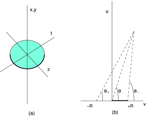
FIG. 1.: (a) The Dirac sheet for a monopole loop in QED. (b) $\theta_{\pm}$ variables for Dirac loops solution.

As for the case of a single monopole, $\partial_{\mu}\varphi=\hat{\varphi}/u$ is singular as one approaches the 3-4 plane, $u\rightarrow 0$. For $v>R$, $\theta_{\pm}\rightarrow 0$, the pre-factor vanishes, and this singularity is absent. However, for $0<v<R$, $\theta_{+}\rightarrow 0$, $\theta_{-}\rightarrow\pi$, the pre-factor approaches 2 and a Dirac sheet is present. We are now ready to generalize this construction to the Maximal Abelian projection in the background of an instanton.

C Monopole Loop in an Instanton Background

Returning to the differential MA conditions, Eq. (15) and Eq. (16), an obvious solution corresponds to the gauge rotation from the singular to the non-singular gauge, $\Omega=g^{\dagger}=(x_{4}+i\vec{x}\cdot\vec{\tau})/|x|$. In the Euler parameterization, this corresponds to $\alpha=\varphi-\psi$, $\gamma=\pi-(\varphi+\psi)$, and $\beta=2\theta\equiv 2\tan^{-1}(u/v)$. However, on surfaces where $\partial_{\mu}\alpha$ is singular ($u=0$ or $v=0$), $\cos\beta=0$ so that no magnetic monopole is formed.

With the gauge choice $\gamma=-\alpha$, the induced potential, $M^{3}_{\mu}$, becomes

$$M_{\mu}^{3}(x)=\frac{1}{e}[1-\cos\beta(x)]\partial_{\mu}\alpha(x).$$ (25)

Note the similarity between this expression and the monopole solutions for QED, Eq. (24). The Dirac sheet is formed on the surface where $\partial_{\mu}\alpha$ becomes singular and $\beta(x)=\pm\pi$. The magnetic current is on the boundary of the Dirac sheet where $\beta$ has a discontinuity.

Consider the ansatz where $\alpha$ and $\beta$ are only functions of $(\varphi,\psi)$ and $(u,v)$ respectively, i.e., $\alpha(\varphi,\psi)$ and $\beta(u,v)$. It can be shown that the first of the two MA conditions, Eq. (15), is solved under this ansatz by

$$\alpha=\varphi-\psi.$$ (26)

It follows from the QED example that a Dirac sheet can be present either in the 1-2 plane, ($v\rightarrow 0$), or the 3-4 plane, ($u\rightarrow 0$), or both. It is sufficient for us to seek solutions where the monopole loops are oriented in the 3-4 plane. Other orientations, including that oriented in the 1-2 plane, can be obtained by performing appropriate $O(4)$ rotations, as we demonstrate in Sec. 3.

Instead of $u$ and $v$, we convert to $x$ and $\theta$, where $x^{2}=u^{2}+v^{2}$ and $\theta=\tan^{-1}(u/v)$, $0\leq\theta\leq\pi/2$. (See Section 4 for further discussion of the ansatz in the u-v coordinate system.) Now Eq. (16) becomes

$$\frac{1}{x^{3}}\partial_{x}(x^{3}\partial_{x}\beta)+\frac{1}{x^{2}\sin 2\theta}\partial_{\theta}(\sin 2\theta\partial_{\theta}\beta)-\frac{2\sin 2\beta}{x^{2}\sin^{2}(2\theta)}+4f(x)\sin^{2}\beta(\cot\beta-\cot 2\theta)=0.$$ (27)

For $G$ to remain finite, one must impose the boundary condition $\sin\beta=0$ at $\theta=0$ and $\theta=\pi/2$. There remains the freedom for $\beta$ to take on values which are integral multiples of $\pi$.

Recall that we are seeking solutions with $A^{\Omega}_{\mu}(x)$ approaching the behavior of the non-singular gauge at the origin, and approaching the behavior of the singular gauge at infinity. We therefore expect a solution with $\beta\simeq 2\theta\>(mod\>\pi)$ for x small and with $\beta\rightarrow 0\>(mod\>\pi)$ at infinity. A monopole loop lying in the 3-4 plane corresponds to a solution where $\beta$ has a discontinuity on the positive $v$-axis. To be precise, we seek solutions where $(i)$ $\beta(x,\pi/2)=0$, $(ii)$ $\beta(x,0)=-\pi$ for $0<x<R$, and $\beta(x,0)=0$ for $R<x<\infty$, and $(iii)$ $\beta(x,\theta)\rightarrow 0$ for $x\rightarrow\infty$.

An analytic solution for $\beta(x,\theta)$ in the limit of small monopole size, $R/\rho\rightarrow 0$ can be found; this will be discussed in Section 3. For general $R/\rho$, the solution to Eq. (27) can be obtained numerically. Using a simple relaxation method for $G$ (described in Section 4), very accurate solution for $\beta$ can be found, as illustrated in Fig 2. Independent of the detailed form of the solution, with $\alpha=\varphi-\psi$, the discontinuity in $\beta(x,\theta=0)$ at $x=R$ leads to a magnetic current,

$$k_{\mu}(x)=\frac{2}{e}\;\delta(x_{1})\delta(x_{2}){\delta(v-R)}\hat{\psi},$$ (28)

where we have re-introduced the charge factor. Therefore our solution corresponds to a loop of monopole with a magnetic charge $g=4\pi/e$ in the instanton background.

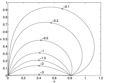
FIG. 2.: Solution to $\beta(u,v)$ for a monopole loop with $R/\rho=0.81$ and $\rho=1$.

In fact we have explored the more general case of a Higgs potential $V(\phi)=\lambda(\phi^{2}-1)^{2}$, where $\phi$ is the magnitude of the Higgs field $\vec{\phi}$. The change in the value of $G$ is almost independent of the parameter $\lambda$. It is now clear that our general monopole loop solutions yield a family of solutions which all satisfy the local MA condition and which interpolate between the singular gauge and the non-singular gauge for an instanton. For $0\leq x<<R$, $\Omega(x)\sim g^{\dagger}(x)$ up to a $U(1)$ rotation; the effect of the gauge transformation is to remove the singularity at $x=0$. Since $\beta\rightarrow 0$ for $x\rightarrow\infty$, it follows that, with $\gamma=-\alpha$, $\Omega\rightarrow I$ rapidly and the large-$x$ behavior of the gauge fields is unchanged. The transition between “small” $x$ and “large” $x$ is marked by the presence of a monopole loop of radius $R$ in the 3-4 plane. As $R$ goes to $\infty$, the monopole loop is pushed to infinity, leaving behind a gauge field configuration which is the instanton in the non-singular gauge.

There is in fact a very large manifold of solutions. In addition to the loops described above, one can clearly impose the boundary conditions for $\beta$ to jump by $\pm\pi$ on either the $\theta=0$ axis or the $\theta=\pi/2$ axis or both, at arbitrary radii $R_{i}$. So long as the final value of $\beta$ as $x^{2}\rightarrow\infty$ is set to be the same multiple of $\pi$ on both boundaries, no ”topological charge has been pushed to the spatial infinity and the functional $G$ will still be finite. This will give a series of concentric loops with increasing radii and magnetic charge either $g$ or $-g$. In addition as describe in Sec 4, the application of Lorentz invariance to these solutions will re-orient these loops in 4-d space.

III Collective Coordinates and Stability of Monopole Loop

In this section, we first address the question concerning the degeneracy of the monopole loop solutions constrained to a fixed radius $R$ in the instanton background. This analysis closely parallels the discussion of the collective coordinates for the instanton itself. The Yang-Mills action is invariant under the 15-parameter conformal and the 3-parameter global $SU(2)$ groups. However, an instanton solution breaks 8 of these symmetries leading to 8 collective coordinates, roughly identified as 4 for its location, 1 for its size, and 3 for its isospin orientation, (see below for a more precise definition.) A monopole solution in each instanton background with these 8 coordinates held fixed further breaks some of the remaining 10 symmetries, leading to additional collective coordinates for the orientation of the loop.

Next we will address the dependence of the loop solution on the loop radius $R$. Each solution is a stationary point of the gauge fixing functional under the constraint of fixed radius. To restrict further the MA projection, one may also impose the condition that $G$ is a global minimum. We therefore need to study $G(R)$, $0\leq R<\infty$, and determine if there is a true minimum for a finite non-vanishing value of loop radius $R$. We shall show that, for a large instanton with size $\rho$, (or equivalently small monopole loops with radii $R<<\rho$), there is a very weak dependence of the gauge fixing functional $G$ in $R$, so the scale of the loops is “nearly” a collective coordinate. This near zero mode leads to “marginal instability” for the formation of small monopole loops.

A $O(4)$ Invariance and Orientation of the Monopole loop

The fact that we constructed the monopole loop solution lying in the 3-4 plane is purely for mathematical convenience; a larger family of loop solutions can be obtained by applying $O(4)$ Lorentz transformations. Since $SO(4)=SU_{L}(2)\times SU_{R}(2)$, it is possible to define two sets of mutually commuting angular momentum generators by $L_{L}^{a}=-(i/2)\bar{\eta}^{a}_{\mu\nu}x^{\mu}\partial_{\nu}$ and $L_{R}^{a}=-(i/2)\eta^{a}_{\mu\nu}x^{\mu}\partial_{\nu}$. (In terms of the conventional “rotation” and “boost” operators, $\vec{J}$ and $\vec{K}$, one has $\vec{L}_{L}=[\vec{J}-\vec{K}]/2$ and $\vec{L}_{R}=[\vec{J}+\vec{K}]/2$.) Using the spinor basis, it is trivial to show that an instanton configuration is invariant under an arbitrary rotation in $SU_{R}(2)$, generated by $\vec{L}_{R}$. An instanton is also invariant under an $SU_{L}(2)$ rotation, (generated by $\vec{L}_{L}$), provided that a corresponding isospin rotation is performed simultaneously.

If we consider the kinematics of the loop in the 3-4 plane, ignoring the instanton background for now, clearly rotations in the 1-2 and 3-4 plane leave it invariant. In fact it can be easily shown that these are the only invariances and that the remaining four-parameter coset space $SU_{L}(2)/U_{L}(1)\times SU_{R}(2)/U_{R}(1)$ rotates the loop to an arbitrary plane. Thus the loop breaks both left and right chiral $SU(2)$ factors in the $O(4)$ group, analogous to the way the ’t Hooft-Polyakov monopole breaks the $SU(2)$ isospin group. Since a MA gauge also fixes a direction in the isospin space by identifying $\tau_{3}$, the only remaining symmetry transformations belong to $SU_{R}(2)$. Thus given a monopole loop solution, all other inequivalent solutions can be obtained by performing $O(4)$ rotations belonging to the quotient space $SU_{R}(2)/U_{R}(1)$.

We now provide a few details on these transformations. Any rotation $U\epsilon SU_{R}(2)$, expressed in the conformal coordinates of Eq.(13), acts on $x_{\alpha\dot{\beta}}$ to give $x^{\prime}_{\alpha\dot{\beta}}=x_{\alpha\dot{\beta}^{\prime}}U^{\dagger}_{\dot{\beta}^{\prime}\dot{\beta}}$. Let us see what happens to a circular loop of radius $R$ centered in the 3-4 plane: ${\tt u}_{0}(\sigma)=x_{0}(\sigma)+iy_{0}(\sigma)=0$ and ${\tt v}_{0}(\sigma)=z_{0}(\sigma)+it_{0}(\sigma)=Re^{i\sigma/2}$, where $0\leq\sigma\leq 4\pi$. First consider a rotation, $R_{3}(\lambda)=e^{i\lambda L_{R}^{3}}=e^{i\lambda\tau_{3}/2}$, in the $U(1)$ subgroup of $SU(2)_{R}$. It simultaneously rotates the 1-2 and 3-4 planes by the same angle $\lambda/2$, i.e., ${\tt u}_{0}\rightarrow{\tt u}(\sigma)={\tt u}_{0}(\sigma)e^{-i\lambda/2}$ and ${\tt v}_{0}\rightarrow{\tt v}(\sigma)={\tt v}_{0}(\sigma)e^{-i\lambda/2}$. This clearly leaves a monopole loop lying in the 3-4 plane invariant. Next consider rotations, $R_{2}(\lambda)=e^{i\lambda L_{R}^{2}}=e^{i\lambda\tau_{2}/2}$. Again using conformal coordinates, one finds that

$${\tt u}(\sigma) = \cos(\lambda/2){\tt u}_{0}(\sigma)-\sin(\lambda/2){\tt v}_{0}^{*}(\sigma)=-\sin(\lambda/2)Re^{-i\sigma/2}$$ (29)

$${\tt v}(\sigma) = \cos(\lambda/2){\tt v}_{0}(\sigma)+\sin(\lambda/2){\tt u}_{0}^{*}(\sigma)=\cos(\lambda/2)Re^{i\sigma/2}.$$ (30)

The resulting loop has a circular projections onto the 1-2 and 3-4 planes with radii $R\sin(\lambda/2)$ and $R\cos(\lambda/2)$ respectively. In particular, for $\lambda=\pi$, it rotates a loop in the 3-4 plane to one lying in the 1-2 plane, as promised. Finally, consider a general $SU_{R}(2)$ rotation. Since it can be parameterized using Euler’s angles as $U(\lambda_{3},\lambda_{2},\lambda_{3}^{\prime})=R_{3}(\lambda_{3})R_{2}(\lambda_{2})R_{3}(\lambda_{3}^{\prime})$, one finds that the resulting loop is given by

$${\tt u}(\sigma)=-R\sin(\lambda_{2}/2)e^{-i(\sigma+\lambda_{3}-\lambda^{\prime}_{3})/2},\>\>\>\>{\tt v}(\sigma)=R\cos(\lambda_{2}/2)e^{i(\sigma-\lambda_{3}-\lambda^{\prime}_{3})/2}.$$

For $\lambda_{3}\not=0$, although the projections onto the 1-2 and 3-4 planes remain circular, it is no longer circular for projections onto other planes, e.g., the 1-4 plane. Clearly, all distinct loops can be characterized by two independent angles, parameterized by $\lambda_{3}$ and $\lambda_{2}$.

Given a fixed isospin orientation for an instanton, the average over the loop orientation tensor $N_{\mu\nu}$ can now be found. For instance, for the standard isospin orientation given by Eq. (5), the monopole loop solution lying in the 3-4 plane is characterized by an anti-symmetric tensor $N_{\mu\nu}=(\delta_{\mu,3}\delta_{\nu,4}-\delta_{\mu,3}\delta_{\nu,4})$. Averaging over $SU_{R}(2)$, one finds that

$$<N_{\mu\nu}>={\textstyle{1\over 2}}[(\delta_{\mu,3}\delta_{\nu,4}-\delta_{\mu,3}\delta_{\nu,4})-(\delta_{\mu,1}\delta_{\nu,2}-\delta_{\mu,2}\delta_{\nu,1})].$$ (31)

In a random dilute instanton gas, this implies a correlation between the monopole loops and the isospin orientation of the associated instanton. As discussed in the Conclusion this correlation may provide a signature of our mechanism for loop formation in the QCD vacuum.

B Limit of Small Monopole Loop

Classically $SU(2)$ gauge theory in four-dimension has no dimensionful parameter, so the instanton solution breaks scale invariance through the introduction of the width $\rho$. Consequently our monopole solutions depends on the dimensionless ratio $\rho/R$, and we may consider the solutions in the limit for small loops size, $\rho/R\rightarrow\infty$. Let us return to Eq. (27), where the width parameter $\rho$ enters through the function $f(x)=\rho^{2}/[x^{2}(x^{2}+\rho^{2})]$. After scaling both $x$ and $\rho$ by $R$, one finds that the equation is greatly simplified in the limit $\rho/R\rightarrow\infty$, $f(x)\rightarrow x^{-2}$.

In this limit, an exact monopole loop solution to Eq. (27) is

$$\beta(x,\theta)=\beta_{0}(x,\theta)\equiv 2\theta-(\theta_{+}+\theta_{-})+\pi,$$ (32)

with $\theta_{\pm}=\tan^{-1}[u/(v\pm R)]$, as defined for the earlier QED example with a monopole loop in the 3-4 plane. Note that $\beta_{0}=0$ on the u-axis, and it has a jump by $\pi$ on the v-axis at $v=R$, ($\beta_{0}=-\pi$ for $0<v<R$ and $\beta_{0}=0$ for $R<v<\infty$). This solution is valid provided that $0<R<<\rho$. The Dirac sheet lies in the 3-4 plane bounded by the circle of radius $R$ where the monopole current resides.

In the limit of small monopole loop and for $0\leq x<<R$, the function $\beta\simeq 2\theta-\pi$ and therefore $\beta$ is not “small”. This reflects the fact that $\Omega\simeq g^{\dagger}(x)$ in the limit $x\rightarrow 0$, so it is singular at the origin. On the other hand, outside of the monopole loop radius, $R<x<\infty$, $\beta$ scales with $R$. Therefore in this “outer region”, for $R\rightarrow 0$, $\beta$ admits an expansion in $(R^{2}/x^{2})$ as

$$\tan\beta\sim\tan\beta_{0}=\frac{-R^{2}\sin(2\theta)}{x^{2}-R^{2}\cos(2\theta)}\sim-\sin(2\theta)(\frac{R^{2}}{x^{2}})+0(\frac{R^{4}}{x^{4}}).$$ (33)

Consequently for fixed $x$ and $x\not=0$, the limit of small monopole loop is characterized by “small” gauge transformations. This allows us to examine the stability of monopole solutions by a linear analysis about $\phi^{a}(x)\sim\delta_{a,3}$.

C Marginal Stability of the Small Monopole

Our monopole solutions are stationary values of $G$ constrained by the boundary condition to a fixed radius $R$. We therefore proceed to study the functional $G(R)$ evaluated at the the loop solution in the range $0\leq R<\infty$. Near $R\rightarrow\infty$, $G(R)$ is monotonically increasing since $G$ is divergent for an instanton in the non-singular gauge. For $R$ small, a leading order monopole solution is known. Initially we had hoped that $G(R)$ has a minimum for some fixed $R>0$. However in spite of our best effort, variational calculations have so far led to results where $G(R)$ is always monotonically increasing. This is also confirmed by very accurate numerical integration of our 2-d PDE’s as described in Sec. 4. We are now convinced that the strong MA projection defined by the global minimum of the functional $G$ is simply the singular gauge itself, which can be viewed as the limit of a monopole loop with radius shrinks to zero. Using our small radius solutions for $\beta$, we are able to analyze the small $R$ behavior for $G(R)$.

We now consider in detail the region near to $R=0$. Assuming that $R=0$ is a minimum, one would expect that $G(R)\sim\rho^{2}[\delta_{0}+\delta_{1}(R/\rho)^{2}+\cdots\cdots]$, with $\delta_{1}>0$. It came initially as a surprise that we found $\delta_{1}=0$. This suggests the possibility of a zero mode in the stability equation around the singular gauge.

Let us expand $G[\phi]$ to quadratic order in the neighborhood of $\vec{\phi}_{0}=(0,0,1)$, parameterized by $\vec{\phi}\simeq\vec{\phi}_{0}+\vec{\omega}$,

$$G[\phi]\simeq G[\phi_{0}]+{\textstyle{1\over 4}}\int d^{4}x\vec{\omega}\cdot{\cal M}\vec{\omega},$$ (34)

where the constraint $|\vec{\phi}|^{2}=1$ is realized to this order by having $\vec{\omega}\cdot\vec{\phi}_{0}=0$, i.e., $\vec{\omega}$ only has 2 transverse components. The stability of small oscillations is studied by finding eigenvalues of a hermitian operator,

$${\cal M}\omega_{i}=\lambda_{i}\omega_{i},$$ (35)

where

$${\cal M}=-{\partial_{x}}^{2}-{3\over x}{\partial_{x}}-{4\over x^{2}}{\vec{L}_{L}}^{2}-8f(x)T^{3}L_{L}^{3}\;,$$ (36)

with $\vec{L}_{L}$ as generators of $SU_{L}(2)$ and $\vec{T}$ of isospin rotations in the adjoint representation.

Expanding $\vec{\omega}$ in terms of these normalized eigenvectors, $\vec{\omega}=\sum_{i}\vec{a}_{i}\omega_{i}$, one has $G[\phi]\simeq G[\phi_{0}]+{\textstyle{1\over 4}}\sum_{i}\lambda_{i}|\vec{a}_{i}|^{2}$. With $R=0$ as a minimum for $G$, stability requires all eigenvalues are non-negative, i.e., $\lambda_{i}\geq 0$. One would also expect that an infinitesimal loop is “nucleated” along the direction $\vec{\omega}$ of the eigenvector with the lowest eigenvalue, $\lambda_{0}$, and $\vec{a}_{0}=0(R)$. It follows that $\delta_{1}\propto\lambda_{0}$. The fact that our numerical treatment indicates that $\delta_{1}\simeq 0$ as depicted in Fig. 3, (described in Sec. 4) implies that $\lambda_{0}=0$, i.e., to quadratic order there is a zero mode. We now try to construct this zero mode.

With $\vec{\omega}$ in the 1-2 plane, $T^{3}$ takes on eigenvalues $t_{3}=\pm 1$. Since ${\cal M}$ commutes with $\vec{L}_{L}^{2}$, $L_{L}^{3}$, and $T^{3}$, there are a family of eigenvalues $\{\lambda_{i}\}$ for each set of $\{l(l+1),l_{3},t_{3}\}$, $l=0,1,2,\cdots\cdots$, $-l\leq l_{3}\leq l$, and they can be found by solving an ordinary differential equation,

$$\{-{\partial_{x}}^{2}-{3\over x}{\partial_{x}}+{4l(l+1)\over x^{2}}-8t_{3}l_{3}f(x)\}\Psi(x)=\lambda\Psi(x),$$

where $\Psi$ is the “radial” part of the eigenfunction. With $f(x)>0$, the attractive case corresponds to $l_{3}t_{3}=1$ and the lowest energy level is $l=1$. We find that all eigenvalues are positive, except possibly one. This zero eigenvalue solution can be constructed by changing variable to $z=1/x^{2}$, and solving

$$[-{d^{2}\over dz^{2}}+V_{eff}(z)]\Psi=\lambda z^{-3}\Psi,$$ (37)

where $V_{eff}(z)=2/z^{2}-2/z^{3}f({1/\sqrt{z}})=2\rho^{-2}/(z+\rho^{-2})$. The zero eigenvalue solution is

$$\Psi(x)=(1+\frac{1}{x^{2}})-(1+\frac{x^{2}}{2})\log(1+\frac{1}{x^{2}}).$$ (38)

The $x\rightarrow\infty$ limit is $\Psi(x)\rightarrow x^{-4}$ as it must. But the $x\rightarrow 0$ limit is $\Psi(x)\rightarrow x^{-2}$, which leads to logarithmic divergence in the norm at short distances. This divergence seems to render this “near” zero mode questionable. However, it should be recognized that our “small loop” solution (33) is valid only for $R<x<\infty$. A proper treatment of our small oscillations problem requires cutting out a small ball around the origin, with a radius $r_{0}=O(R)$. Moreover, because of the zero eigenvalue the divergence in the norm does not imply a divergence in $G$. We should in principle be able to solve this problem by find the lowest eigenvalue and then letting $r_{0}$ go to zero. With respect to this cutoff, our “near” zero mode is physically meaningful. An alternative approach, which is under investigation, may be to use the more general MA gauge with a Higgs potential. This has a natural length scale $1/m_{H}$, which probably provides the necessary cutoff at short distances.

As one extends beyond the quadratic approximation, one can see that this zero mode leads to our “exact solution” in the special case of $f=1/x^{2}$. That is, the formal $\rho\rightarrow\infty$ limit solution. In this sense, it is easy to see that the divergence should be cut off by $\rho$. For the exact solution, the eigenvalue is of the order $(R/\rho)^{2}\log(\rho/R)$, which is consistent with our numerical calculation as exhibited in Fig. 3.

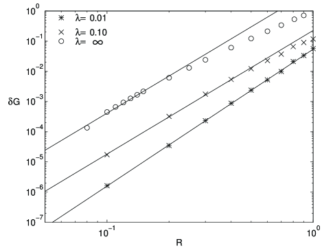
FIG. 3.: For $\lambda=0.01,0.10,\infty$, the change in the Gauge fixing functional $G$ as a function of the monopole loop radius $R$.

IV Numerical Solutions to MA Projection

For a general value of the monopole loop radius $R$, we were unable to find an analytic solution. Consequently we have discretized our PDE’s and found numerical solutions. The need for a numerical integration method is not surprising since even the ’t Hooft-Polyakov monopole has no known solution in closed form, except in the BPS limit.

With the simplifying ansatz (26), we were able to reduce the problem from a 4-d to a 2-d set of PDE’s allowing us to construct very accurate solutions on a 2-d grid. To check the validity of this ansatz, we also consider the standard 4-d hypercubic grid conventionally used in Monte Carlo studies of non-Abelian gauge field theory. An important advantage of the 4-d grid is the ability of making a global search for stationary points. However this numerical integration method should not be confused with Monte Carlo simulations. Here the grid is used merely to solve numerically the classical PDE’s of Yang-Mills theory. As always for discretization methods, it is important to consider carefully errors arising from the grid spacing $a$ and the volume of the box. Our analysis of these errors will shed some light on earlier investigations [15, 16, 17] of the Abelian projection in “cooled” instanton configurations.

A Single Instanton Case

Once we have made our ansatz (26), $\beta(x,y,z,t)$ only depends on two “radial” co-ordinates: $u=\sqrt{x^{2}+y^{2}}$ and $v=\sqrt{z^{2}+t^{2}}$. This feature also generalizes to the case of the MA projections (8) with a Higgs potential which allows the magnitude $\phi(x,y,z,t)\equiv|\vec{\phi}|$ to fluctuate. Here our ansatz (26) implies that both $\beta(x_{\mu})$ and $\phi(x_{\mu})$ depend only on $u$ and $v$. The functional $G$ takes the simple from

$$G=4\pi^{2}\int dudv\;uv\;[{\textstyle{1\over 2}}M(\beta)\phi^{2}+{\textstyle{1\over 2}}(\partial_{\mu}\phi)^{2}+{\textstyle{1\over 4}}\lambda(\phi^{2}-1)^{2}]\;,$$ (39)

where $\phi(u,v)=|\phi|$, $(\partial_{\mu}\phi)^{2}=(d\phi/du)^{2}+(d\phi/dv)^{2}$ and

$$M(\beta)=8f(x^{2})+(d\beta/du)^{2}+(d\beta/dv)^{2}+\sin^{2}\beta(\frac{1}{u^{2}}+\frac{1}{v^{2}})-8f(x^{2})[\sin^{2}\beta-{\textstyle{1\over 2}}\sin\beta\cos\beta(\frac{v}{u}-\frac{u}{v})].$$

The conventional MA gauge is given in the limit $\lambda\rightarrow\infty$.

We introduce grids in u and v, mapping the infinite $u-v$ plane to a finite region, for a range of values of $R/\rho$ and $\lambda$ (see Fig. 3). For all $\lambda$ (including the BPS limit $\lambda=0$), we found that the monopole loop solution exists and that the functional $G$ increases as $R^{4}$ within errors. For all values of $\lambda$ the global minima appeared to be at the point where $R\rightarrow 0$ and the instanton returned to the singular gauge. If we perturbed the background field slightly away from a pure instanton by changing the functional form, $f(x)=\rho^{2}/[x^{2}(x^{2}+\rho^{2})]$, one can easily find field configurations in the same topological sector which stabilized the loop at a fix radius. This strongly suggests that quantum fluctuations or instanton interactions can cause monopole loop formation.

To make a global search for minimal solutions for the MA projection and to verify our theoretical ansatz, we have resorted to a 4-d grid. A natural choice is the standard Wilson approach with link variables,

$$U_{\mu}(x)=e^{\textstyle{iaA_{\mu}(x)}},$$ (40)

where $a$ is the lattice spacing. On this grid the MA functional which leaves the Maximal Abelian subgroup $U(1)$ unconstrained is

$$G=\frac{1}{2}\;a^{2}\;\sum_{\mu,x}\{1-\frac{1}{2}Tr(\hat{\phi}(x)U_{\mu}(x)\hat{\phi}(x+\mu)U_{\mu}(x)^{\dagger})\}.$$ (41)

In order to numerically approximate its value, we restrict the summation over a finite volume V around the origin with open boundary conditions on the surface. This is a good approximation for an isolated instanton, since the contributions to the sum for large $x$ drops as $1/x^{2}$. Furthermore to obtain a finite value for $G$ in the infinite volume limit, we know that the gauge rotation must become a constant at infinity. The minimization of the restricted functional was done using the standard over-relaxation algorithm [24].

The instantons are placed on the grid in the non-singular gauge and then rotated to singular form. Each link is approximated by its integral using the trapezoid rule. The resulting configurations gave topological charge and action deviating at worst by $10\%$ from their continuum values, $1$ and $2\pi^{2}$ respectively.

We have investigated a range of different sizes of lattices and instantons. As expected [15, 16], we have found monopole loop formation in the Maximal Abelian gauge. But our monopole radii do not scale with the instanton size. This is a clear signal that the stabilization of the monopole loop is a lattice artifact. Despite that, we find that once a loop is formed the gauge rotation accurately satisfies our theoretical ansatz (26) that $\alpha=\varphi-\psi$ and $\beta$ depends only on $u$ and $v$.

A finite volume and finite spacing analysis has been done in order to further establish the fact that the monopole loops is a lattice artifact. We measure the change,

$$\Delta(\rho/a,L)=\frac{G_{MA}-G_{instanton}}{G_{instanton}}\;,$$ (42)

of the MA functional after gauge fixing and we demonstrate that it vanishes in the combined limit of infinite volume and zero lattice spacing. In order to show this, we have found a series of solutions for lattice sizes $20^{4}$, $22^{4}$, $24^{4}$, $26^{4}$, $28^{4}$, $30^{4}$ and $32^{4}$ with a fixed instanton size. The infinite volume limit is obtained by doing a linear extrapolation in $1/L$ , where $L=V^{1/4}$ is the linear dimension of our lattice. Fig. 4(a) shows this extrapolation for $\rho/a=4$. The second extrapolation to zero lattice spacing is done from these extrapolated values of $\Delta$ for various values of the instanton radius $\rho$. At infinite volume, the only scale in the problem is $\rho$, and it is therefore defines the lattice spacing, $a\sim 1/\rho$. Thus one takes the $a\rightarrow 0$ limit by taking the $\rho/a\rightarrow\infty$ limit. This extrapolation is done using instanton sizes $\rho/a=3,4,5,6,7$.

The results are shown in Fig. 4(b). The extrapolated value of $\Delta(\rho/a,L)$ in the limit of $a\rightarrow 0$ and $L\rightarrow\infty$ is clearly zero within the numerical error. Another indication that the global minimum of the MA functional is the instanton in the singular gauge is the fact that $\Delta$ is so small $O(10^{-3})$. This is also supported by our experience with the minimizing routine. Starting with the gauge background for an instanton in the singular gauge, it took very few iterations to converge which shows that the displacement of the minimum due to lattice artifacts is actually very small.

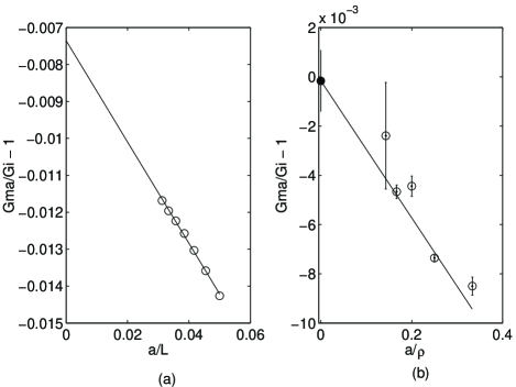
FIG. 4.: The finite lattice spacing and finite volume dependence for the monopole loop solution on the lattice.(a) Typical Infinite volume extrapolation.(b) $a\rightarrow 0$ extrapolation.

B Solutions for Instanton Pairs.

We have also used our 4-d grid to begin to investigate solutions to the MA projection in the background of interacting instanton pairs. For example, we have begun to study instantons (I-I) pairs and instanton anti-instantons pairs (I-A) with various sizes, relative separations and relative isospin orientations. Already several general conclusions can be drawn. The I-I pairs appear to be very similar to the case of single instantons. Indeed for the ’t Hooft ansatz, one can again show that the two instanton solutions (or indeed the multi-instanton solution),

$$\vec{A}_{\mu}\cdot\vec{\tau}=\tau^{\alpha}\bar{\eta}^{\alpha}_{\mu\nu}\partial_{\nu}ln(1+\rho_{1}^{2}/x_{1}^{2}+\rho_{2}^{2}/x_{2}^{2}),$$ (43)

already satisfies the MA gauge condition. On the 4-d grid our preliminary study indicates that the MA projection of the two instantons have small loops centered at each instanton which again appear to be due entirely to lattice artifacts. It is natural to ask whether there is a general property of all exact classical solutions that the global minimum of the MA projection has no monopole trajectories.

On the other hand, we have computed the MA projection for I-A pair with isospins oriented in the most attractive configuration. In this case, contrary to the single instanton and I-I pair large loops are formed in the MA projection. At large separation, each instanton in the I-A pair has its own monopole loop as illustrated in Fig 5, but as the separation $d$ is decreased the individual loops fuse at $d/\rho\simeq 1.88$ to form a large loop which surrounds the I-A pair. These loops clearly scale with the size of the system and the reduction of the MA functional is clearly larger. Further more this reduction in $G$ becomes larger as you approach the continuum limit. Although we have not yet finished the same detailed finite size and finite lattice spacing analysis as in the single instanton case, we have considerable evidence that this effect will survive in the continuum.

In the dipole interactions between I-A pairs, we believe we are seeing the first semi-classical mechanism for nucleating monopole loops. As the instantons become denser, the monopole loops begin to percolate between the individual instantons. It is easy to imagine that in an instanton liquid there is a critical density at which the percolation clusters are infinite and the monopoles can be said to condense. This effect is an intriguing possibility for a semi-classical mechanism for confinement. Additional studies of monopole trajectories for interacting instantons and further analysis to support (or refute) this scenario are postponed to a future publication [18].

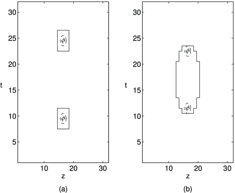
FIG. 5.: Monopole loops for I-A molecule with the most attractive orientation: (a) Loops stabilized at separation $d/\rho=1.88$. (b) Loops fusion at separation $d/\rho=1.38$.

V Conclusions

The main goal of this paper was to find the earliest point in the semi-classical instanton vacuum in which the ’t Hooft Mandelstam monopole appears. We believe that this is the formation of small current loops centered at each instanton and anti-instanton. In the extreme limit of infinite separation, i.e., an isolated instanton, the loops shrink to zero. However to $O(R^{4}\log R)$ in the radius there is a flat direction for loop formation in the gauge fixing functional. We have begun to investigate the effect of instanton anti-instanton interactions. Here it appears that when the relative isospin orientation of an instanton anti-instanton (I-A) pair is most attractive, the monopole loops are stabilized at a finite radius and as the pair moves closer together the individual loops fuse.

There is much more to learn about the mechanism for loop stabilization and the effects of instanton interactions. For the most part we postpone this to a future publication [18]. However it is worth posing some of the questions and extending several arguments touched on early.

First we have noticed that the single instanton in the singular gauge already satisfies the differential form of the MA gauge and gives rise to a finite contribution to the gauge fixing functional $G$. In fact it is trivial to see that all multi-instanton configurations that satisfy the ’t Hooft ansatz $A^{a}_{\mu}=\bar{\eta}^{a}_{\mu\nu}\partial_{\nu}ln(1+F(x^{2}))$ likewise satisfy the MA gauge with a finite contribution for $G$. Thus it is tempting to conjecture that any exact self-dual classical solution minimizes this functional without explicit monopole currents. We are investigating this conjecture further. In this scenario the essential mechanism for monopole loop formation would be the interaction terms between self-dual and anti-self-dual regions that act as the “domain walls” between I-A pairs.

Next it is worth expanding a little on the relationship between the topological charge and the monopole charge for an isolated instanton. In the singular gauge, when we write the topological charge, $Q=(1/16\pi^{2})\int d^{4}xTr[\tilde{F}_{\mu\nu}F_{\mu\nu}]$, in terms of the gauge variant current, $Q=\int d^{4}x\partial_{\mu}K_{\mu}$, one must exclude singular regions. Indeed via Gauss’ theorem, the flux into these excluded singularities gives the net topological charge. We have studied carefully how this theorem is satisfied in the presence of our monopole loop. In the singular gauge, we may write the instanton as

$$A_{\mu}=\bar{A}_{\mu}+M_{\mu}=-\frac{g^{\dagger}\partial_{\mu}g}{i}\frac{x^{2}}{x^{2}+\rho^{2}}+\frac{g^{\dagger}\partial_{\mu}g}{i}.$$ (44)

As we shrink a small sphere toward the origin $x^{2}=\delta^{2}\rightarrow 0$ the surface area is $O(\delta^{3})$. However one sees that the singular part of the current,

$$K_{\mu}=\frac{1}{8\pi^{2}}\epsilon_{\mu\nu\rho\lambda}Tr[A_{\nu}(\partial_{\rho}A_{\lambda}-i{\textstyle{{2}\over{3}}}A_{\rho}A_{\lambda})],$$ (45)

diverges as $O(1/\delta^{3})$ and that the contribution to $Q$ comes entirely from the pure gauge piece, $M_{\mu}$. On the other hand as we rotate the field configuration into a monopole loop,

$$M_{\mu}\rightarrow M_{\mu}=\frac{\Omega g^{\dagger}\partial_{\mu}(\Omega g^{\dagger})^{\dagger}}{i}\;,$$ (46)

the singularity is spread out to the loop at radius $x^{2}=R^{2}$. Now the toroidal surface area around the loop is $O(R\delta^{2})$, but again a careful analysis shows that the only divergent piece of $O(1/\delta^{2})$ comes from $M_{\mu}$. The argument is completely general for a monopole loop gauge and it requires the magnetic charge to be quantized to match the topological charge. This shows that the monopole loop has a very natural fit to the instanton.

Finally we have found that when an isospin orientation of an isolated instanton is fixed, the monopole loops are constrained to a portion of the full $O(4)$ group. Again there is a rather remarkable “coincidence” this time between the symmetries of the monopole loop and the instanton. A single loop “kinematically” breaks the Lorentz group $SU_{L}(2)\times SU_{R}(2)$ into a factor of coset spaces $SU_{L}(2)/U_{L}(1)\times SU_{R}(2)/U_{R}(1)$ in the same sense that the ’t Hooft-Polyakov monopole brakes the $SU(2)$ isospin symmetry down to $SU(2)/U(1)$. Then if we fix the isospin axis of the instanton (anti-instanton) and choose the MA gauge relative to $\tau_{3}$, the loop is only re-oriented by the right (or left) coset. This implies a correlation between the plane of the loop and the isospin orientation, which can be tested in typical background configurations of instantons generated in a Monte Carlo simulation. In this way we can determine whether or not our conjecture that these monopole loops are important configurations for the full quantum theory is correct.

In conclusion, although there are many more details worth considering there is a remarkable coincidence between the form of an instanton and its monopole loop in the MA projection. This is reflected in topological, symmetry and stability terms. This leads us to see the instanton in a new light as the “seed” for the formation of monopole loops. The dynamical implications are much more difficult, but it appears that I-A interactions may play a crucial role and the large “entropy” of monopole loops percolating between near by instantons suggest a promising direction for future research on electric confinement.

A Gauge Covariant Formulation of the Abelian projection

The usual way to study the MA gauge is to applying the gauge transformation to the field,

$$A_{\mu}(x)\rightarrow A^{\Omega}_{\mu}(x)=\Omega(x)A_{\mu}(x)\Omega^{\dagger}(x)\;+\;\frac{1}{ie}\Omega(x)\partial_{\mu}\Omega^{\dagger}(x)\;.$$ (A1)

and find that rotation $\Omega(x)$ which satisfies a gauge condition. Alternatively, one may introduce an auxiliary adjoint Higgs-like field, $\Phi=\vec{\phi}\cdot\vec{\tau}$, expressing the entire problem in a gauge invariant form. We refer to this two methods as “active” and “passive” respectively. In this appendix, we collect together basic formalism for each form.

In the passive description, the MA gauge is cast in a gauge covariant form familiar to the Higgs [25] model, with the entire formalism re-expressed exactly in the form used to construct the ’t Hooft-Polyakov monopole. This covariant formulation both simplifies our analysis and emphasizes the important physical point that the Maximal Abelian projection needs not be viewed as a gauge fixing prescription but rather as a way to define magnetic degrees of freedom. We prefer the latter interpretation.

1 Active View of MA Gauge and Magnetic Current

In the active form, the resulting Abelian field $a_{\mu}(x)=Tr[\tau_{3}A^{\Omega}_{\mu}(x)]$, (or more properly its derivatives), which depends on the choice on the non-Abelian background field, can have singularities leading to a non-zero magnetic current. Introducing the notation, $\bar{A}_{\mu}(x)\equiv\Omega(x)A_{\mu}(x)\Omega^{\dagger}(x)$ and $M_{\mu}(x)\equiv(1/ie)\Omega(x)\partial_{\mu}\Omega^{\dagger}(x)$, the transformed field becomes

$$A^{\Omega}_{\mu}(x)=\bar{A}_{\mu}(x)\;+\;M_{\mu}(x).$$ (A2)

This splits the Abelian field into two components, $a_{\mu}(x)=\bar{A}^{3}_{\mu}(x)+M^{3}_{\mu}(x)$. The first term, $\bar{A}_{\mu}^{3}$, for our problem, comes from a direct rotation of the instanton field. The second “induced” term, $M^{3}_{\mu}$, can contain monopoles as its source when appropriate conditions are met as we demonstrate next.

The Abelian field strength, $f_{\mu\nu}\equiv\partial_{\mu}a_{\nu}-\partial_{\nu}a_{\mu}$, is given by

$$f_{\mu\nu}=(\Omega F_{\mu\nu}\Omega^{\dagger})_{3}-ie[\Omega(A_{\mu}+\frac{1}{ie}\partial_{\mu})\Omega^{\dagger},\Omega(A_{\nu}+\frac{1}{ie}\partial_{\nu})\Omega^{\dagger}]_{3}$$ (A3)

where $(\cdots)_{3}=Tr[\tau_{3}\cdots]$. It again is split into two pieces,

$$f_{\mu\nu}=(\partial_{\mu}\bar{A}^{3}_{\nu}-\partial_{\nu}\bar{A}^{3}_{\mu})+(\partial_{\mu}M^{3}_{\nu}-\partial_{\nu}M^{3}_{\mu}).$$ (A4)

Since the dual of the first combination is obviously divergentless, only the second term contributes to a non-vanishing magnetic current,

$$k_{\mu}(x)=\frac{e}{8\pi}\epsilon_{\mu\nu\rho\sigma}Tr(\tau_{3}\partial_{\nu}[M_{\rho}(x),M_{\sigma}(x)]),$$ (A5)

where $k_{\mu}={\textstyle{{1}\over{4\pi}}}\partial_{\nu}\tilde{f}_{\nu\mu}$, and $\tilde{f}_{\nu\mu}={\textstyle{1\over 2}}\epsilon_{\mu\nu\rho\sigma}f_{\rho\sigma}$.

2 Gauge Invariant View of MA Projection

We now reformulate the MA projection in passive form. Let us begin by noting that the functional,

$$G={{\textstyle{1\over 4}}}\int(A^{1}_{\mu}+iA^{2}_{\mu})(A^{1}_{\mu}-iA^{2}_{\mu})d^{4}x$$ (A6)

is just the mass term in the broken phase of an $SU(2)$ Georgi-Glashow model. This suggests a change of variables from $\Omega(x)$ to

$$\Phi(x)=\Omega^{\dagger}(x)\tau_{3}\Omega(x).$$ (A7)

The functional $G$ now takes form of action for a Higgs field,

$$G={\textstyle{1\over 2}}\int d^{4}x\{{\textstyle{1\over 2}}[D_{\mu}(A)\vec{\phi}]^{2}+V(\vec{\phi}^{2})\},$$ (A8)

where $\Phi=\vec{\phi}\cdot\vec{\tau}$, $D_{\mu}\phi^{a}\equiv\partial_{\mu}\phi^{a}+e\epsilon^{abc}A_{\mu}^{b}\phi^{c}$, and the potential,

$$V(\vec{\phi}^{2})=\sigma(\vec{\phi}^{2}-1),$$ (A9)

involves a Lagrange multiplier $\sigma$ in order to maintain the constraint $\vec{\phi}\cdot\vec{\phi}=1$. We also suggest a generalization of the MA projection to include the standard quartic Higgs potential,

$$V(\vec{\phi}^{2})={\textstyle{1\over 4}}\lambda(\vec{\phi}^{2}-v^{2})^{2},$$ (A10)

with $\Phi(x)$ now given by $\vec{\phi}(x)\cdot\vec{\tau}/|\vec{\phi}(x)|$. This more general from we will refer to as the “Higgs MA projection”. Thus the MA gauge is precisely the same as minimizing the action for a non-dynamical (or auxiliary) Higgs-like field in a background Yang-Mills theory. The limit $\lambda\rightarrow\infty$ at fixed VEV $v$ results in the usual MA projection. This is the limit which takes the Higgs mass $m_{H}$ to infinity. This formulation corresponds to a passive description of a gauge transformation. In the active description, rotation $\Omega$ is applied directly to the gauge field in Eq. (3) so that $\hat{\phi}\rightarrow(0,0,1)$. Clearly, the passive and the active descriptions are equivalent: each specifies a gauge transformation $\Omega$ up to the $U(1)$ subgroup. However the passive description is more “natural” since $\hat{\phi}$ lives in the coset space.

The Abelian field strength (A3) now takes a manifestly gauge invariant form,

$$f_{\mu\nu}=\hat{\phi}^{a}F^{a}_{\mu\nu}-ie\epsilon^{abc}\hat{\phi}^{a}D_{\mu}\hat{\phi}^{b}D_{\nu}\hat{\phi}^{c},$$ (A11)

and the magnetic current is the well known conserved topological current,

$$k_{\mu}(x)=\frac{1}{8\pi e}\epsilon_{\mu\nu\rho\sigma}\epsilon^{abc}\partial_{\nu}\hat{\phi}^{a}\partial_{\rho}\hat{\phi}^{b}\partial_{\sigma}\hat{\phi}^{c}.$$ (A12)

The essential identity in deriving these expressions from our earlier equations is $\partial_{\mu}\Phi=i[\Omega^{\dagger}M_{\mu}\Omega,\Phi]$. An alternative form for $f_{\mu\nu}$ follows directly from Eq. (A4),

$$f_{\mu\nu}=\partial_{\mu}\bar{A}^{3}_{\nu}-\partial_{\mu}\bar{A}^{3}_{\nu}-ie\epsilon^{abc}\hat{\phi}^{a}\partial_{\mu}\hat{\phi}^{b}\partial_{\nu}\hat{\phi}^{c}.$$ (A13)

This approach to MA projection not only provides a gauge invariant treatment, but also allows a topological interpretation for the possible presence of magnetic sources. For example, as in the case of the ’t Hooft-Polyakov monopole, the presence of a monopole charge can be understood to be due to a non-trivial homotopy $\Pi_{2}(SU(2)/U(1))=Z$.

3 Higgs MA Projection for Instanton

For general reference to our analysis, we final give the full set of differential equation for the Higgs MA projection,

$$D_{\mu}(A)^{2}\vec{\phi}-\vec{\nabla}_{\phi}V(\phi)=0\;.$$ (A14)

The two independent PDE’s for the tangential components, now take the form

$$\phi\;\partial^{2}_{\mu}\alpha+2\partial_{\mu}\phi\partial_{\mu}\alpha+2\phi\;\cot\beta\;(\partial_{\mu}\alpha)(\partial_{\mu}\beta)=-2[\phi(\hat{\phi}\cdot\vec{A}_{\mu})\;(\partial_{\mu}\beta)-(\hat{\beta}\cdot\vec{A}_{\mu})\;(\partial_{\mu}\phi)],$$ (A15)

$$\phi\partial^{2}_{\mu}\beta+2\partial_{\mu}\phi\partial_{\mu}\beta-{\textstyle{1\over 2}}\phi\;\sin 2\beta\;(\partial_{\mu}\alpha)^{2}=2[\phi\sin\beta(\hat{\phi}\cdot\vec{A}_{\mu})\;(\partial_{\mu}\alpha)-(\hat{\alpha}\cdot\vec{A}_{\mu})(\partial_{\mu}\phi)],$$ (A16)

by projecting Eq. (11) onto the $\hat{\alpha}(x)$ and $\hat{\beta}(x)$ axes respectively. In addition there is a new equation for the radial mode,

$$\partial_{\mu}^{2}\phi=-\{2[\sin\beta(\hat{\beta}\cdot\vec{A}_{\mu})(\partial_{\mu}\alpha)+(\hat{\alpha}\cdot\vec{A}_{\mu})\partial_{\mu}\beta]+[V^{\prime}(\phi^{2})-{\textstyle{{2}\over{3}}}\vec{A}^{2}_{\mu}]\}\phi.$$ (A17)

Under our ansatz, $\alpha=\varphi-\psi$, with $\beta(u,v)$ and $\phi(u,v)$ only functions of $u$ and $v$, Eq. (A15) is still satisfied automatically. Now Eq. (A16) becomes

$$\phi\partial^{2}_{\mu}\beta+2(\partial_{u}\phi\partial_{u}\beta+\partial_{v}\phi\partial_{v}\beta)-(\frac{u^{2}+v^{2}}{2u^{2}v^{2}})\phi\sin(2\beta)=$$

$$2f(x)\{\phi[(\frac{v^{2}-u^{2}}{uv})\sin^{2}\beta-\sin 2\beta]+[v\partial_{u}\phi-u\partial_{v}\phi]\},$$ (A18)

and the the radial equation (A17) becomes

$$\partial_{\mu}^{2}\phi=-\{f(x)[\sin 2\beta(\frac{v^{2}-u^{2}}{uv})+4\sin^{2}\beta+2(u\partial_{v}\beta-v\partial_{u}\beta)]+[V^{\prime}(\phi^{2})-{\textstyle{{2}\over{3}}}\vec{A}^{2}_{\mu}]\}\phi.$$ (A19)

Both analytical and numerical properties of these equations are discussed in the text. There appears to be remarkably little dependence of our monopole loop solution on $\lambda$ from $\lambda=0$ (the BPS limit) to $\lambda=\infty$ (the standard MA projection).

4 Abelian Projected Theory

In the MA gauge, one is left with an intermediate description of a $U(1)$ gauge theory,

$${\cal L}(a_{\mu},A^{\pm}_{\mu})={\textstyle{1\over 4}}f_{\mu\nu}^{2}+(d_{\mu}A^{+}_{\nu})(d_{\mu}A^{-}_{\nu})+e^{2}(A^{+}_{\mu}A^{-}_{\nu}-A^{+}_{\nu}A^{-}_{\mu})A^{+}_{\mu}A^{-}_{\nu}.$$ (A20)

interacting exclusively through charged vectors $A^{\pm}=A^{1}_{\mu}\pm iA^{2}_{\mu}$. The $U(1)$ covariant derivative is $d_{\mu}=\partial_{\mu}+iea_{\mu}$.

In addition to the standard Wilson loop $W({\cal C})=Tr{\cal P}_{\cal C}e^{\textstyle{i\int dx_{\mu}A_{\mu}}}$, one may introduce the Abelian Wilson loop,

$$W^{ab}({\cal C})=e^{\textstyle{i\int dx_{\mu}a_{\mu}}}$$ (A21)

which in turn can be split up into “photon” and “monopole” factors

$$W^{ab}({\cal C})=\exp[\;i\int dx_{\mu}\bar{A}^{3}_{\mu}\;]\;\;\;\exp[ie\int\int d\sigma_{\mu\nu}\epsilon^{abc}\hat{\phi}^{a}\partial_{\mu}\hat{\phi}^{b}\partial_{\nu}\hat{\phi}^{c}].$$ (A22)

The second integral is taken over any surface whose boundary is given by the loop ${\cal C}$. The near “saturation” of the non-Abelian string tension by the Abelian part in the MA gauge, $\sigma_{ab}\simeq.92\sigma$, and the Abelian part by the monopole contribution, $\sigma_{monopole}\simeq.95\sigma_{ab}$, observed in lattice simulations [28] is referred to as Abelian Dominance. If this survives the continuum limit this may provide the dynamical link between monopole configuration and confinement.

To understand the role that Abelian dominance might play in the continuum theory, it is useful to look at the very interesting form of the Wilson loop suggested by Diakonov and Petrov [29],

$$W({\cal C})=\int{\cal D}\hat{\phi}(x)\exp[i{\textstyle{1\over 2}}\int dx_{\mu}\hat{\phi}\cdot\vec{A}_{\mu}]\;\;\;\exp[\int d\sigma_{\mu\nu}\epsilon^{abc}\hat{\phi}^{a}\partial_{\mu}\hat{\phi}^{b}\partial_{\nu}\hat{\phi}^{c}].$$ (A23)

A comparison with the Abelian Wilson loop in the MA gauge shows that this has exactly the same form with the additional step that one must average over all gauge transformation in the $SU(2)/U(1)$ coset. Consequently Abelian dominance is the statement that in the true quantum vacuum, the contributions to the $\hat{\phi}$ average is approximated by the MA projection. Thus one strategy to proving confinement is to first establish Abelian dominance (or more precisely the inequality $W({\cal C})\leq W^{ab}({\cal C})$ for large loops) and then to demonstrate that monopole condensation occurs forcing an area law for the Abelian loop.

REFERENCES

- [1] G. ’t Hooft, Phys. Rev. Lett. 37, 8 (1976); Phys. Rev D14, 3432 (1976).
- [2] E.V. Shuryak, Nucl. Phys. B302, 559-644 (1988).
- [3] E. Witten, Nucl. Phys. B156, 269 (1979); G. Veneziano, Nucl. Phys. B159, 213 (1979).
- [4] M.-C. Chu, J.M. Grandy, S. Huang, J.W. Negele, Phys. Rev. D49, 6093 (1994); Phys. Rev. D48, 3340 (1993).
- [5] S. Mandelstam, Phys. Rep. C23, 245 (1976).
- [6] G. ’t Hooft, Nucl. Phys. B190 (1981) 455.
- [7] M. E. Peskin , Ann. of Phys. 113, 122 (1978).
- [8] A. Polyakov Phys. Lett. B59, 82 (1975); Nucl. Phys. B120, 429 (1977).
- [9] N. Seiberg and E. Witten, Nucl. Phys. B426, 19 (1994).
- [10] M. I. Polikarpov, Lattice 96 Review talk hep-lat/9609020 (1996).
- [11] A. A. Belavin, A. M. Polyakov, A. S. Schwartz and Tyupkin, Phys. Lett. B59, 85 (1975); M. F. Attyah, N. J. Hitchin, V. G. Drinfeld and Yu. I. Manin, Phys. Lett. A65, 185 (1978).
- [12] H. Suganuma, A. Tanaka, S. Sasaki, O. Miyamura, Nucl. Phys. B(Proc. Supp.), Proc. of Lattice 95; H. Suganuma, K. Itakura, H. Toki, HEPTH-9512141, (hep-th/9512141).
- [13] P. Rossi, Nucl. Phys. B149, 170 (1979).
- [14] M.N. Chernodub and F.V. Gubarev ITEP-95-34, hep-th/9506026.
- [15] A. Hart and M. Teper Oxford preprint No: OUTP-95-44-P, hep-lat/9511016.
- [16] V. Bornyakov, G. Schierholz DESY 96-069, HLRZ 96-22, hep-lat/9605019 ; G. Schierholz DESY 95-127 HLRZ 95-35.
- [17] H. Markum, W.Sakuler, S. Thurner, Nucl. Phys B (Proc. Supl. LATTICE95 ), 254 (1995) (hep-lat/9510024); S. Thurner, M. Feurstein, H. Markum, W. Sakuler, Phys. Rev D54 3457(1996).
- [18] R. C. Brower, K. Orginos and C-I Tan, “Monopole loops for interacting instantons”, (in preparation).
- [19] A. S. Kronfeld, G. Schierholz and Wiese, Nucl. Phys. B293, 461 (1987).
- [20] R. Rajaraman, Solitons and Instantons, (North-Holland Publishing Company, 1982).
- [21] A. Belavin, A. Polyakov, A. Schwartz and Y. Tyupkin, Phys. Lett. B59, 85 (1975).
- [22] R. Jackiw, C. Nohl, C. Rebbi, Phys. Rev. D15 No 6, 1642 (1977).
- [23] M. Blagojevi’c and P. Senjanovi’c, Phys. Rep. 157, Nos 4 & 5, 233 (1988).
- [24] J. E. Mandula, M. Oglivie, Phys. Lett. B248, 156 (1990).
- [25] A. S. Kronfeld, M. L. Laursen, G. Schierholz and Wiese, Phys. Lett. B198 No 4, 516 (1987).
- [26] M.N. Chernodub, M.I. Polikarpov, A.I. Veselov, Ahrenshoop Symp. 307 (1995) (hep-lat/9512030); T.L. Ivanenko, A.V. Pochinsky, M.I. Polikarpov, Nucl. Phys. B, (Proc. Suppl. 30 ), 565 (1993); M.N. Chernodub, M.I. Polikarpov, A.I. Veselov, Trento QCD Workshop, 81 (1995) (hep-lat/9512008).
- [27] J. Smit and A. J. van der Sijsm Nucl. Phys. B355, 603 (1991).
- [28] G. S. Bali, V. Bornyakov, M. Mueller-Preussker, and K. Schilling, hep-lat/960312, to be published in Phys. Rev. D.
- [29] D.I.Diakonov and V.Yu. Petrov, Phys. Lett. B 224 (1989) 131.