FAU-TP3-96/15

The Path Integral for 1+1-dimensional QCD

O. Jahn, T. Kraus and M. Seeger

Institut für Theoretische Physik,
Friedrich-Alexander-Universität Erlangen-Nürnberg,
Staudtstraße 7, 91058 Erlangen

We derive a path integral expression for the transition amplitude in 1+1-dimensional QCD starting from canonically quantized QCD. Gauge fixing after quantization [1] leads to a formulation in terms of gauge invariant but curvilinear variables. Remainders of the curved space are Jacobians, an effective potential, and sign factors just as for the problem of a particle in a box. Based on this result we derive a Faddeev-Popov like expression for the transition amplitude avoiding standard infinities that are caused by integrations over gauge equivalent configurations.

1 Introduction

The standard Faddeev-Popov path integral formulation [2] provides a convenient framework for calculations in the perturbative regime of QCD. There are, however, some points of interest that need clarification:

• The derivation of the Faddeev-Popov path integral involves infinities from the integration over gauge equivalent configurations. Therefore it would be preferable to find a derivation of a QCD path integral which is well-defined at all stages.

• The usual Faddeev-Popov formulation in the continuum gives no prescription for how to handle infrared singularities, which may play an essential role for the non-perturbative aspects of QCD.

• There is a lively discussion about the detailed form of the Faddeev-Popov path integral, concerning issues like Jacobian factors and the appearance of the Haar measure [1, 3, 4, 5, 6].

In order to clarify these issues we choose canonically quantized QCD as a well-defined starting point. By working in 1+1 dimensions we avoid field theoretical infinities indicating the need for regularization; only infinities resulting from gauge invariance are left. We derive a path integral expression for the transition amplitude in the traditional manner by inserting eigenstates of the gauge field operators and coherent states for the fermions respectively. With the help of a gauge fixing procedure following Lenz et al. [1], we achieve formulations purely in terms of physical (i.e. unconstrained) but curvilinear variables. We derive two equivalent expressions for the path integral depending on the domain of definition (compact vs. non-compact) of the remnants of the gauge fields. The inclusion of fermions entails no further difficulties and is treated in the appendix. As an illustration of the formalism we explicitly calculate the partition function and the spectrum of pure SU($N_{\rm c}$) Yang-Mills theory. Finally we establish the connection to the Faddeev-Popov formalism avoiding the usual infinities.

To make the paper self-contained and to fix our notation we first summarize the formalism.

2 Review of the Canonical Formalism and Conventions

In this section we give a short review of the formulation of 1+1-dimensional Yang-Mills theory in the canonical formalism, based on the work of Lenz, Naus and Thies [1].

The Hamiltonian of 1+1-dimensional Yang-Mills theory in the Weyl gauge is given by

$$H=\int_{0}^{L}{\rm d}x\mathop{\rm Tr}\nolimits\bigl{(}\Pi(x)\bigr{)}^{2},$$ (1)

where $\Pi(x)$ is the momentum canonically conjugate to $A(x)$, and equals, up to a sign, the chromo-electric field. $A(x)$ and $\Pi(x)$ are ${\rm su}(N_{\rm c})$ matrices, that can be expanded in terms of the $N_{\rm c}^{2}-1$ standard generators $\lambda^{a}/2$,

$$A(x)=A^{a}(x)\frac{\lambda^{a}}{2}\quad\mbox{and}\quad\Pi(x)=\Pi^{a}(x)\frac{\lambda^{a}}{2}.$$ (2)

(Repeated indices are summed over throughout the paper.) Space is assumed to be a circle, i.e., periodic boundary conditions $A(x+L)=A(x)$ and $\Pi(x+L)=\Pi(x)$ are imposed. The theory is quantized by demanding the commutation relations

$$[\Pi^{a}(x),A^{b}(y)]=-{\rm i}\delta^{ab}\delta(x-y),$$ (3)

where $\delta(x-y)$ denotes a periodic $\delta$-function.

In the Weyl gauge, Gauß’s law has to be required as a constraint on physical states,

$${\rm D}\Pi\mathopen{|}\Phi\rangle=0,\qquad\mbox{where }{\rm D}^{ab}=\delta^{ab}\frac{\partial}{\partial x}+gf^{acb}A^{c}.$$ (4)

Since the operator ${\rm D}\Pi$ generates small gauge transformations, this means that physical wave functions have to be gauge invariant. (In 1+1 dimensions there are no large gauge transformations because $\pi_{1}({\rm SU}(N_{\rm c}))$ is trivial.)

The Gauß law constraint is solved in [1] by a transition to curvilinear coordinates $(a,A^{\prime})$, where the coordinates $a$ constitute a maximal set of gauge invariant quantities, while $A^{\prime}$ represents the gauge variant part of $A$. Thus, physical wave functions are functions of $a$ only. More specifically, $a$ is defined as a constant diagonal matrix containing the phases of the eigenvalues of the Wilson loop around the circle:

$${\rm e}^{{\rm i}gLa}\equiv V^{\dagger}{\cal P}\exp\left({\rm i}g\int_{0}^{L}{\rm d}x\,A(x)\right)V,$$ (5)

where $\cal P$ denotes path ordering and $V\in{\rm SU}(N_{\rm c})$ is chosen such that

$$a={\rm diag}(a_{1},\dots,a_{N_{\rm c}})=a^{c_{0}}\frac{\lambda^{c_{0}}}{2}.$$ (6)

Because only $N_{\rm c}-1$ of the $N_{\rm c}$ variables $a_{i}$ are independent, $a$ is expanded in terms of the $N_{\rm c}-1$ generators of the Cartan subalgebra of ${\rm SU}(N_{\rm c})$ in the last equation.

As can be seen from (5), the variables $a$ are defined only up to

$$\bullet \mbox{displacements}\quad a_{i}\longrightarrow a_{i}+\frac{2\pi}{gL}k_{i}\quad\mbox{for }k_{i}\in{\bf Z}\mbox{ with }\sum_{i}k_{i}=0\quad$$ (7)

$$\bullet \mbox{and color permutations}\quad a_{i}\longrightarrow a_{P(i)}\quad\mbox{for }P\in{\rm S}_{N_{\rm c}},\quad$$ (8)

where S${}_{N_{\rm c}}$ denotes the symmetric group. The set of all displacements will sometimes be denoted by ${\cal D}$, the set of all color permutations by ${\cal W}$ (the ‘Weyl group’ of ${\rm SU}(N_{\rm c})$). Examples for the cases of SU(2) and SU(3) are shown in figs. 1 and 2, resp.

Figure 1: Fundamental domain for SU(2). FD denotes the fundamental domain, the dashed arrow is a displacement, the dotted arrow (a reflection at the origin) is a color permutation

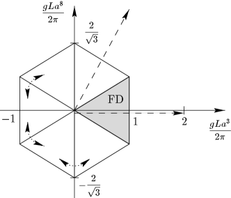
Figure 2: Fundamental domain for SU(3). The shaded area is the fundamental domain, the dashed arrows are displacements and the dotted arrows (reflections at the diagonals of the hexagon) are color permutations

The invariant hyperplanes of all reflections contained in ${\cal D}\times{\cal W}$ divide ${\bf R}^{N_{\rm c}-1}$ into domains in such a way that any $a\in{\bf R}^{N_{\rm c}-1}$ can be mapped into a given domain by exactly one transformation in ${\cal D}\times{\cal W}$. To render the definition of $a$ unique, one can therefore restrict its values to one of the domains, which is then called the fundamental domain (FD). A special choice for SU(2) and SU(3) is shown in figs. 1 and 2.

The remaining coordinates $A^{\prime}$ can be chosen such that the Jacobian of the coordinate transformation factorizes,

$$\frac{\partial(a,A^{\prime})}{\partial(A)}=J(a)J^{\prime}[A^{\prime}],$$ (9)

where $J(a)$ results only from the diagonalization in (5) and equals the density of the ‘radial’ (class) part of the Haar measure of ${\rm SU}(N_{\rm c})$,

$$J(a)=\prod_{i<j}\sin^{2}\left(\frac{gL(a_{i}-a_{j})}{2}\right).$$ (10)

In the new coordinates the Hamiltonian (1), when acting on physical states, reduces to the radial part of the Laplace-Beltrami operator of ${\rm SU}(N_{\rm c})$,

$$H\mathopen{|}\Phi\rangle = H_{\rm ph}\mathopen{|}\Phi\rangle,$$

$$H_{\rm ph} \equiv -\frac{1}{2L}\frac{1}{J(a)}\frac{\partial}{\partial a^{c_{0}}}J(a)\frac{\partial}{\partial a^{c_{0}}}.$$ (11)

We are now in a position to formulate the path integral for this problem. We will derive two forms with different domains of $a$:

1. $a$ is defined on the covering space ${{\bf R}}^{N_{\rm c}-1}$.

2. $a$ is restricted to the FD and all integrations are performed over the FD.

In the first case the transformations (7) and (8) will be considered as residual symmetries, under which physical wave functions have to be invariant.

3 Derivation of the Path Integral on the Covering Space

In this section we derive a path integral expression for the time evolution of a physical state $|\Phi\rangle$, i.e. for the amplitude $\langle A|\Phi(t)\rangle$, on the covering space.

As usual, we divide the time interval into a large number $N$ of time slices, each of length $\varepsilon=t/N$ and insert unity at each step,

$$\langle A|\,{\rm e}^{-{\rm i}Ht}|\Phi\rangle=\int\prod_{i=1}^{N}\left[{\rm d}A_{i-1}\,\langle A_{i}|\,{\rm e}^{-{\rm i}H_{\rm ph}\varepsilon}|A_{i-1}\rangle\right]\langle A_{0}|\Phi\rangle,$$ (12)

with the identification $A_{N}\equiv A$. In (12) $H$ has been replaced by $H_{\rm ph}$ using (11) and the fact that $H$ commutes with the projection onto physical states.

The matrix elements for the infinitesimal time evolution are now evaluated in a Schrödinger representation where we pay attention to the fact that the coordinate transformation yielded a non-trivial Jacobian,

$$\langle A_{i}|\,{\rm e}^{-{\rm i}H_{\rm ph}\varepsilon}|A_{i-1}\rangle=\exp\left[{\rm i}\varepsilon\frac{1}{2L}\left(\frac{\partial^{2}}{\partial{a_{i}^{c_{0}}}^{2}}+f_{c_{0}}(a_{i})\frac{\partial}{\partial a_{i}^{c_{0}}}\right)\right]\times{}$$ (13)

$$\quad\quad\quad\quad\quad\quad\quad\quad{}\times\frac{\delta(a_{i}-a_{i-1})}{\sqrt{J(a_{i})J(a_{i-1})}}\frac{\delta[A^{\prime}_{i}-A^{\prime}_{i-1}]}{\sqrt{J^{\prime}[A^{\prime}_{i}]J^{\prime}[A^{\prime}_{i-1}]}}.$$

The Jacobians have been split in such a way that we can obtain a simpler form of the kinetic energy by moving one of the factors through the differential operators. But before this we have to ensure differentiability of the terms the operators act on, which can be achieved by use of the identity

$$\frac{\delta(a_{i}-a_{i-1})}{\sqrt{J(a_{i})J(a_{i-1})}}=\frac{\mathop{\rm sgn}\nolimits a_{i}}{\sqrt{J(a_{i})}}\,\frac{\mathop{\rm sgn}\nolimits a_{i-1}}{\sqrt{J(a_{i-1})}}\,\delta(a_{i}-a_{i-1}),$$ (14)

where $\mathop{\rm sgn}\nolimits a$ equals $+1$ if an even number of reflections is needed to map $a$ into the FD and $-1$ otherwise. This sign makes the root of the Jacobian differentiable:

$$\mathop{\rm sgn}\nolimits a\,\sqrt{J(a)}=\mathop{\rm sgn}\nolimits a\,\prod_{k<l}\left|\sin\frac{gL(a_{l}-a_{k})}{2}\right|\propto\prod_{k<l}\left(\sin\frac{gL(a_{l}-a_{k})}{2}\right).$$ (15)

If we now move the Jacobian factors to the left, the kinetic energy simplifies and an effective potential is induced,

$$\exp\left[{\rm i}\varepsilon\frac{1}{2L}\left(\frac{\partial^{2}}{\partial{a^{c_{0}}}^{2}}+f_{c_{0}}(a)\frac{\partial}{\partial a^{c_{0}}}\right)\right]\frac{\mathop{\rm sgn}\nolimits a}{\sqrt{J(a)}}=\frac{\mathop{\rm sgn}\nolimits a}{\sqrt{J(a)}}\exp\left[{\rm i}\varepsilon\left(\frac{1}{2L}\frac{\partial^{2}}{\partial{a^{c_{0}}}^{2}}-V_{\rm eff}\right)\right],$$ (16)

which is of course reminiscent of the hydrogen atom where $V_{\rm eff}$ would be the centrifugal barrier. The procedure just applied corresponds to the transition to “reduced” wave functions. Here, however, $V_{\rm eff}$ can be calculated to yield an irrelevant constant [1]. It follows that

$$\langle A_{i}|\,{\rm e}^{-{\rm i}H_{\rm ph}\varepsilon}|A_{i-1}\rangle=\frac{\delta[A^{\prime}_{i}-A^{\prime}_{i-1}]\cdot\mathop{\rm sgn}\nolimits a_{i}\cdot\mathop{\rm sgn}\nolimits a_{i-1}}{\sqrt{J(a_{i})J(a_{i-1})J^{\prime}[A^{\prime}_{i}]J^{\prime}[A^{\prime}_{i-1}]}}\,(2\pi)^{1-N_{\rm c}}\times{}$$ (17)

$$\quad\quad\quad\quad\quad\quad{}\times\int\limits_{{\bf R}^{N_{\rm c}-1}}{\rm d}p_{i}\,\exp\left[{\rm i}\varepsilon\left(p_{i}\frac{a_{i}-a_{i-1}}{\varepsilon}-\frac{1}{2L}p_{i}^{2}-V_{\rm eff}\right)\right],$$

where the integral representation of the $\delta$-function has been inserted and the index $c_{0}$ has been supressed from $p$ and $a$.

Let us now consider the projection onto physical states. Simply requiring them to be independent of the $A^{\prime}$ with $a$ varying over the whole ${\bf R}^{N_{\rm c}-1}$ is not sufficient to render them physical. In addition, we have to postulate invariance under displacements and color permutations. A physical state would therefore be, e.g.

$$|\Phi\rangle=|a\rangle_{\rm phys}\equiv\sum_{\omega\in{\cal W}\times{\cal D}}|{}^{\omega}a\rangle.$$ (18)

After insertion into (12) this leads to the phase space path integral

$$\langle a_{\rm f}|\,{\rm e}^{-{\rm i}H_{\rm ph}t}|a_{\rm i}\rangle_{\rm phys}=\frac{1}{\sqrt{J(a_{\rm f})J(a_{\rm i})}}\sum_{\omega}\mathop{\rm sgn}\nolimits\omega\int\limits_{{\bf R}^{N_{\rm c}-1}}\prod_{i=1}^{N-1}{\rm d}a_{i}\,(2\pi)^{(1-N_{\rm c})N}\times{}$$ (19)

$${}\times\int\limits_{{\bf R}^{N_{\rm c}-1}}\prod_{i=1}^{N}{\rm d}p_{i}\,\exp\left[{\rm i}\varepsilon\sum_{i=1}^{N}\left(p_{i}\frac{a_{i}-a_{i-1}}{\varepsilon}-\frac{1}{2L}p_{i}^{2}-V_{\rm eff}\right)\right]\Biggr{|}_{{\textstyle a}_{0}={\textstyle a}_{\rm i}}^{{\textstyle a}_{N}={\textstyle{}^{\omega}a}_{\rm f}},$$

where we have assumed that $a_{\rm f},a_{\rm i}\in{\rm FD}$ and have performed the integration over the unphysical degrees of freedom with help of

$$\int{\rm d}A\,(.)=\int{\rm d}a\,J(a)\int{\rm d}A^{\prime}\,J^{\prime}[A^{\prime}]\,(.).$$ (20)

In eq. (19) only the $\mathop{\rm sgn}\nolimits\omega$ factors of the endpoints are left, while all others have canceled pairwise. The configuration space path integral is obtained by performing the Gaussian integrations over the momenta,

$$\langle a_{\rm f}|\,{\rm e}^{-{\rm i}H_{\rm ph}t}|a_{\rm i}\rangle_{\rm phys}=\frac{1}{\sqrt{J(a_{\rm f})J(a_{\rm i})}}\left(\frac{L}{2\pi{\rm i}\varepsilon}\right)^{(N_{\rm c}-1)N/2}\sum_{\omega}\mathop{\rm sgn}\nolimits\omega\times{}$$ (21)

$${}\times\int\limits_{{\bf R}^{N_{\rm c}-1}}\prod_{i=1}^{N-1}{\rm d}a_{i}\,\exp\left[{\rm i}\varepsilon\sum_{i=1}^{N}\left(\frac{L}{2}\frac{(a_{i}-a_{i-1})^{2}}{\varepsilon^{2}}-V_{\rm eff}\right)\right]\Biggr{|}_{{\textstyle a}_{0}={\textstyle a}_{\rm i}}^{{{\textstyle a}_{N}={\textstyle{}^{\omega}a}_{\rm f}}},$$

with $a_{\rm f},a_{\rm i}\in{\rm FD}$.

The inclusion of Fermions can be accomplished along similar lines and is therefore postponed to the appendix.

4 Derivation of the Path Integral on the Fundamental Domain

We start with the Schrödinger equation for the reduced wave function $\Psi(a)=\sqrt{J(a)}\,\Phi(a)$:

$$\left(-\frac{1}{2L}\frac{\partial^{2}}{\partial{a^{c_{0}}}^{2}}+V_{\rm eff}\right)\Psi(a)={E}\Psi(a),$$ (22)

together with the condition $\Psi(a)=0$ if $J(a)=0$. Because the reduced wave function has to vanish on the boundary of the FD, the solution of the Schrödinger equation (22) in the FD is not influenced by the solutions in its gauge copies.

We now reformulate the problem. We enforce the vanishing of the wave function on the boundary of the FD by introducing a potential, which is equal to zero inside and infinite outside the FD. Thus we obtain the new Schrödinger equation

$$\left(-\frac{1}{2L}\frac{\partial^{2}}{\partial{a^{c_{0}}}^{2}}+V_{\rm eff}+V_{\rm box}(a)\right)\Psi(a)={E}\Psi(a),$$ (23)

with

$$V_{\rm box}(a)=\left\{\begin{array}[]{r@{\quad:\quad}l}0&a\in{\rm FD}\\ \infty&{\rm otherwise,}\end{array}\right.$$

and no constraint on the reduced wave function $\Psi$.

As we have a standard kinetic energy and a potential which is bounded from below we can apply the Trotter product formula [7]

$${\rm e}^{-{\rm i}H_{\rm ph}t}=\lim_{N\rightarrow\infty}\left({\rm e}^{-{\rm i}\left(V_{\rm eff}+V_{\rm box}(a)\right)t/N}\cdot{\rm e}^{-{\rm i}E_{\rm kin}t/N}\right)^{N},$$ (24)

and then derive the path integral in the usual way. To be consistent with the previous section we consider the reduced $a$-eigenstates $\sqrt{J(a)}\,|a\rangle$ with the property

$$\sqrt{J(a^{\prime})}\,\langle a^{\prime}|a\rangle\sqrt{J(a)}=\delta(a-a^{\prime}).$$ (25)

We obtain

$$\langle a_{\rm f}|\,{\rm e}^{-{\rm i}H_{\rm box}t}|a_{\rm i}\rangle=\frac{1}{\sqrt{J(a_{\rm f})J(a_{\rm i})}}\,\int\limits_{{\bf R}^{N_{\rm c}-1}}\prod_{i=1}^{N-1}{\rm d}a_{i}\,(2\pi)^{(1-N_{\rm c})N}\,\int\limits_{{\bf R}^{N_{\rm c}-1}}\prod_{i=1}^{N}{\rm d}p_{i}\times{}$$

$$\quad\quad\quad\quad\quad\left.{}\times\,\exp\left[{\rm i}\varepsilon\sum_{i=1}^{N}\left(p_{i}\frac{a_{i}-a_{i-1}}{\varepsilon}-\frac{1}{2L}p_{i}^{2}-V_{\rm eff}-V_{\rm box}(a_{i})\right)\right]\right|_{{\textstyle a}_{0}={\textstyle a}_{\rm i}}^{{\textstyle a}_{N}={\textstyle a}_{\rm f}}.$$

Due to the potential $V_{\rm box}$, which is rapidly oscillating outside the FD, the $a$-integration can be restricted to give the phase space path integral on the FD

$$\langle a_{\rm f}|\,{\rm e}^{-{\rm i}H_{\rm box}t}|a_{\rm i}\rangle=\frac{1}{\sqrt{J(a_{\rm f})J(a_{\rm i})}}\,\int\limits_{\rm FD}\prod_{i=1}^{N-1}{\rm d}a_{i}\,(2\pi)^{(1-N_{\rm c})N}\,\int\limits_{{\bf R}^{N_{\rm c}-1}}\prod_{i=1}^{N}{\rm d}p_{i}\times{}$$

$$\quad\quad\quad\quad\quad\quad\quad\quad\quad\left.{}\times\,\exp\left[{\rm i}\varepsilon\sum_{i=1}^{N}\left(p_{i}\frac{a_{i}-a_{i-1}}{\varepsilon}-\frac{1}{2L}p_{i}^{2}-V_{\rm eff}\right)\right]\right|_{{\textstyle a}_{0}={\textstyle a}_{\rm i}}^{{\textstyle a}_{N}={\textstyle a}_{\rm f}}.$$

The configuration space path integral is obtained by performing the Gaussian integrations over the momenta,

$$\langle a_{\rm f}|\,{\rm e}^{-{\rm i}H_{\rm box}t}|a_{\rm i}\rangle=\frac{1}{\sqrt{J(a_{\rm f})J(a_{\rm i})}}\left(\frac{L}{2\pi{\rm i}\varepsilon}\right)^{(N_{\rm c}-1)N/2}\times{}$$

$$\quad\quad\quad\quad\quad\quad\quad{}\times\int\limits_{\rm FD}\prod_{i=1}^{N-1}{\rm d}a_{i}\,\exp\left[{\rm i}\varepsilon\sum_{i=1}^{N}\left(\frac{L}{2}\frac{(a_{i}-a_{i-1})^{2}}{\varepsilon^{2}}-V_{\rm eff}\right)\right]\Biggr{|}_{{\textstyle a}_{0}={\textstyle a}_{\rm i}}^{{\textstyle a}_{N}={\textstyle a}_{\rm f}}.$$

5 Equivalence of the Two Formulations

In the previous sections with have derived two different formulations of the path integral for 1+1-dimensional Yang-Mills theory. We will show now that they are equivalent in the limit $\varepsilon\rightarrow 0$, where we deal with paths which are continuous in time. In the formulation on the covering space we then have a sum over endpoints, which are related by small gauge transformations and are accompanied by a possible minus sign. We demonstrate that only paths which stay within the FD are relevant because all paths that touch the boundary or cross it cancel each other.

To calculate the transition amplitude $\langle a_{\rm f}|\,{\rm e}^{-{\rm i}H_{\rm ph}t}|a_{\rm i}\rangle_{\rm phys}$ we have to sum over all paths starting at $a(0)=a_{\rm i}$ and ending at $a(t)={}^{\omega}a_{\rm f}$ including a sum over the symmetry transformations $\omega$.

Figure 3: Cancellation of Paths

Let $t_{1}=\inf\{\tau\,|\,0<\tau<t,\,a(\tau)\in\partial{\rm FD}\}$ be the first time that $a(\tau)$ touches the boundary of the FD. Now consider the path

$$\tilde{a}(\tau)=\left\{\begin{array}[]{r@{\quad:\quad}l}a(\tau)&0\leq\tau\leq t_{1}\\ {}^{\rho}a(\tau)&t_{1}\leq\tau\leq t,\end{array}\right.$$

where $\rho\in{\cal W}\times{\cal D}$ denotes the reflection at the hyperplane the path $a(\tau)$ meets at $\tau=t_{1}$. Because the reflection at the boundary is a symmetry of the Yang-Mills Hamiltonian, the two paths $\tilde{a}(\tau)$ and $a(\tau)$ have the same action. But as the final points of the two paths differ by a reflection, they have opposite sign and cancel each other in the sum over symmetry transformations in eqs. (19) and (21). Thus it is equivalent to consider only paths which stay inside the FD and we have arrived at the second form (4, LABEL:config2) of the path integral.

For the case of ${\rm SU}(2)$ the cancellation of paths is illustrated in fig. 3.

6 Explicit Calculation of the Transition Amplitude and the Partition Function

To illuminate the role of the sum over endpoints we derive an explicit expression for the transition amplitude (21) in terms of energy eigenstates. The Gaussian integrations in (21) can be readily performed to yield the well-known propagator of a free particle plus a sum over endpoints, a sign and a Jacobian factor:

$$\langle a_{\rm f}|\,{\rm e}^{-{\rm i}H_{\rm ph}t}|a_{\rm i}\rangle_{\rm phys}=\frac{1}{\sqrt{J(a_{\rm f})J(a_{\rm i})}}\left(\frac{L}{2\pi{\rm i}t}\right)^{(N_{\rm c}-1)/2}\sum_{\omega}\mathop{\rm sgn}\nolimits\omega\exp\left[{\rm i}\frac{L}{2t}({}^{\omega}a_{\rm f}-a_{\rm i})^{2}-{\rm i}V_{\rm eff}t\right].$$ (28)

Now we split the sum over $\omega$ into a sum over color permutations $\rho\in{\cal W}$ and a sum over displacements $\delta\in{\cal D}$. The sum over displacements is turned into a sum over momenta by use of Poisson’s resummation formula,

$$\sum_{\delta\in{\cal D}}f(a+\delta)=\frac{1}{|{\rm EC}|}\sum_{p\in{\cal D}^{*}}\,\int\limits_{{\bf R}^{N_{\rm c}-1}}\!\!{\rm d}a^{\prime}\,{\rm e}^{-{\rm i}pa^{\prime}}f(a+a^{\prime}),$$ (29)

where $|{\rm EC}|$ is the volume of the elementary cell (the Wigner-Seitz cell of ${\cal D}$) and ${\cal D}^{*}$ denotes the reciprocal lattice of the Bravais lattice ${\cal D}$. It is defined by

$$p\delta=2\sum_{i=1}^{N_{\rm c}}p_{i}\delta_{i}\in 2\pi{\bf Z}\qquad\mbox{for }\delta_{i}\in\frac{2\pi}{gL}{\bf Z},\ \sum_{i}\delta_{i}=0,$$ (30)

or, since $\sum_{i}p_{i}=0$,

$$p_{i}=\frac{gL}{2}\left(n_{i}-\frac{1}{N_{\rm c}}\sum_{i}n_{i}\right)\qquad\mbox{with }n_{i}\in{\bf Z},\ n_{N_{\rm c}}=0.$$ (31)

Here, following the convention of (6), $p_{i}$ and $\delta_{i}$ denote the diagonal matrix elements of $p$ and $\delta$, resp.

Applying (29) to (28) and performing the $a^{\prime}$-integration we can write

$$\langle a_{\rm f}|\,{\rm e}^{-{\rm i}H_{\rm ph}t}|a_{\rm i}\rangle_{\rm phys}=\frac{1}{\sqrt{J(a_{\rm f})J(a_{\rm i})}\,|{\rm EC}|}\sum_{p\in{\cal D}^{*}}\sum_{\rho\in{\cal W}}\mathop{\rm sgn}\nolimits\rho\exp\left[-{\rm i}\frac{t}{2L}p^{2}+{\rm i}p({}^{\rho}a_{\rm f}-a_{\rm i})-{\rm i}V_{\rm eff}t\right].$$ (32)

The $p$ that are invariant under some permutation $\rho\in{\cal W}$, and therefore also under some transposition $\tau$, do not contribute because for these the exponential is invariant under the substitution $\rho\to\tau\rho$ and therefore each term with a given $\rho$ is canceled by the term with $\tau\rho$. For the other $p$ we choose out of each multiplet of $N_{\rm c}!$ vectors the one with $p_{1}>p_{2}>\ldots>p_{N_{\rm c}}$ and sum over the permuted ones separately. After rearranging the $\rho$-sum we obtain

$$\langle a_{\rm f}|\,{\rm e}^{-{\rm i}H_{\rm ph}t}|a_{\rm i}\rangle_{\rm phys}=\frac{1}{\sqrt{J(a_{\rm f})J(a_{\rm i})}\,|{\rm EC}|}\sum_{\textstyle{p\in{\cal D}^{*}\atop p_{1}>\ldots>p_{N_{\rm c}}}}\sum_{\rho,\sigma\in{\cal W}}\mathop{\rm sgn}\nolimits(\rho\sigma)\times{}$$ (33)

$${}\times\exp\left[-{\rm i}\left(\frac{1}{2L}p^{2}+V_{\rm eff}\right)t\right]{\rm e}^{-{\rm i}p{}^{\rho}\!a_{\rm f}}{\rm e}^{{\rm i}p{}^{\sigma}\!a_{\rm i}}.$$

This formula provides us immediately with the energy spectrum of 1+1-dimensional Yang-Mills theory. Using the representation (31) and the expression for $V_{\rm eff}$ found in [1] one obtains

$$E_{n}=\frac{g^{2}L}{4}\left[\sum_{i=1}^{N_{\rm c}-1}n_{i}^{2}-\frac{1}{N_{\rm c}}\left(\sum_{i=1}^{N_{\rm c}-1}n_{i}\right)^{2}-\frac{N_{\rm c}(N_{\rm c}^{2}-1)}{12}\right]$$ (34)

with $n_{1}>n_{2}>\ldots>n_{N_{\rm c}-1}>0$. For SU(2) this reads

$$E_{n}=\frac{g^{2}L}{8}(n_{1}^{2}-1)$$ (35)

and for SU(3)

$$E_{n}=\frac{g^{2}L}{6}(n_{1}^{2}+n_{2}^{2}-n_{1}n_{2}-3).$$ (36)

The corresponding eigenfunctions can also be read off:

$$\Phi_{p}(a)=\frac{1}{\sqrt{J(a)|{\rm EC}|}}\sum_{\rho\in{\cal W}}\mathop{\rm sgn}\nolimits\rho\,{\rm e}^{{\rm i}p{}^{\rho}\!a}.$$ (37)

These are just the characters of the irreducible representations of SU($N_{\rm c}$). We see that the sum over color permutations together with the sign ensures that the zeros of the Jacobian are canceled and the wave functions remain finite.

Our results agree with those of Rajeev [8], Gupta et al. [9], Engelhardt [10], Engelhardt and Schreiber [11] and the compact formulation of Hetrick [5] but disagree with the non-compact formulation appearing in the latter. In this formulation the gauge is fixed on the classical level and the resulting configuration space, the Cartan subalgebra of SU($N_{\rm c}$) modulo the Weyl group, is quantized under the assumption of a flat measure. As opposed to this, in Rajeev’s as well as in our (resp. [1]’s) approach the full constrained system is quantized, and in the course of implementing the constraints the configuration space turns out to be the set of classes of SU($N_{\rm c}$) (the eigenvalues of the Wilson loop) equipped with the Haar measure, which is induced by the flat measure of the original (unconstrained) configuration space.

In an earlier work [6] Hetrick and Hosotani derive the non-compact results also via a Faddeev-Popov path integral and find that the Haar measure (the Faddeev-Popov determinant) is canceled by the $A^{0}$-integration. In section 7 we will show that our result is equivalent to a Faddeev-Popov-like expression with an additional antisymmetrizing sum over gauge copies and that the Haar measure is indeed canceled. The calculation in this section shows that these eliminate that part of the spectrum that differs between their and our approach.

The partition function

$$Z(\beta)=\mathop{\rm Tr}\nolimits{\rm e}^{-\beta H}=\int_{\rm FD}{\rm d}a\,J(a)\,\langle a|\,{\rm e}^{-\beta H_{\rm ph}}|a\rangle_{\rm phys},$$ (38)

where the trace is taken only over the physical part of the Hilbert space, contains a matrix element that differs from the transition amplitude calculated in section 3 only by a factor of ${\rm i}$ in the exponent. The derivation of (21) and (33) is still valid after the replacement of ${\rm i}t$ by $\beta$ and ${\rm i}\varepsilon$ by $\varepsilon$, and so we obtain, after inserting (33) into (38) and performing the integration,

$$Z(\beta)=\sum_{\textstyle{p\in{\cal D}^{*}\atop p_{1}>\ldots>p_{N_{\rm c}}}}\exp\left[-\beta\left(\frac{1}{2L}p^{2}+V_{\rm eff}\right)\right].$$ (39)

7 Connection with the Faddeev-Popov Formalism

Having derived the gauge fixed path integral, one is tempted to ask for the connection between this approach and the more conventional Faddeev-Popov approach. In this section we show that the two expressions for the partition function are actually equivalent if the infrared degrees of freedom in the Faddeev-Popov path integral are treated correctly. To this end we continue the transition amplitude (21) with endpoints identified to Euclidean space and insert the result into (38):

$$Z(\beta)=\int_{\rm FD}{\rm d}a^{1}(0)\,\sum_{\omega}\mathop{\rm sgn}\nolimits\omega\int_{a^{1}(0)}^{{}^{\omega}\!a^{1}(0)}{\cal D}a^{1}\exp\left[-\int_{0}^{\beta}{\rm d}\tau\left(\frac{L}{2}(\dot{a}^{1})^{2}-V_{\rm eff}\right)\right]$$ (40)

Here we have adopted the usual continuum notation for the path integral measure and integrand. In addition, we have reintroduced the spatial Lorentz index on $a$.

The axial gauge corresponds to the gauge condition $f[A]=0$ with

$$f^{c_{0}}[A]=\partial_{1}A^{1c_{0}}+\frac{1}{L}a^{0c_{0}},\quad f^{c}[A]=A^{1c}\quad(c\neq c_{0}),$$ (41)

where $a^{0}$ denotes the diagonal part of the spatial zero mode of $A^{0}$. Note that we cannot require the zero mode of $A^{1c_{0}}$ to vanish because of the periodic boundary conditions. Instead we use the remaining gauge freedom to eliminate $a^{0}$.

Now we use (41) to introduce the integration over $a^{0}$ and the missing modes of $A^{1}$ in (40),

$$Z(\beta)\propto\int{\cal D}a^{0}\sum_{\omega}\mathop{\rm sgn}\nolimits\omega\int\limits_{\hbox to0.0pt{\hss$\scriptstyle A^{1}(\beta)={}^{\omega}\!A^{1}(0)\atop\scriptstyle a^{1}(0)\in{\rm FD}$\hss}}{\cal D}A^{1}\,\delta[f[A]]\exp\left[-\int_{0}^{\beta}{\rm d}\tau\int{\rm d}x\left(\frac{1}{2}(\dot{A}^{1})^{2}-\frac{V_{\rm eff}}{L}\right)\right],$$ (42)

where we have suppressed $\det\partial_{1}$. $A^{1}$ contains $a^{1}$ as a Cartesian zero mode, and the two integrals in (40) are contained in the integral over $A^{1}$. In the shorthand notation ${}^{\omega}\!A^{1}$ the transformation $\omega$ is understood to act only on the diagonal part of the spatial zero mode of $A^{1}$. In the exponent $a^{1}$ has been replaced with $A^{1}$ due to the gauge condition incorporated by the $\delta$-function.

As the next step we generate the remaining modes of the time component of the gauge field via the identity

$$1=\det{\rm D^{\prime}_{1}}\int{\cal D}^{\prime}A^{0}\,\exp\left[-\int_{0}^{\beta}{\rm d}\tau\int{\rm d}x\left(\frac{1}{2}\left({\rm D_{1}}A^{0}\right)^{2}+\dot{A}^{1}{\rm D_{1}}A^{0}\right)\right],$$ (43)

which is valid under the gauge condition. The symbol ${\cal D}^{\prime}A^{0}$ means that the zero modes of the covariant derivative D₁ are not included in the integral.

Next we want to show that the Faddeev-Popov determinant is already contained in the factors appearing in (42) and (43). It can be calculated by looking at the change of the the gauge condition under an infinitesimal gauge transformation,

$$\Delta_{f}[A]=\det\left(\frac{\delta f}{\delta\beta}\right)_{\beta=0}.$$ (44)

One obtains

$$\delta f^{c_{0}}=\frac{1}{g}\partial_{1}\left({\rm D}^{1}\delta\beta\right)^{c_{0}}+\frac{1}{gL^{2}}\int{\rm d}x\left({\rm D}^{0}\delta\beta\right)^{c_{0}},\quad\delta f^{c}=\frac{1}{g}\left({\rm D}^{1}\delta\beta\right)^{c}\quad(c\neq c_{0}),$$ (45)

and therefore

$$\Delta_{f}[A]\propto\det{\rm D}^{1\prime},$$ (46)

which is, up to a constant factor, what we found above.

The full expression therefore reads

$$Z(\beta)\propto\sum_{\omega}\mathop{\rm sgn}\nolimits\omega\int\limits_{\hbox to0.0pt{\hss$\scriptstyle A^{1}(\beta)={}^{\omega}\!A^{1}(0)\atop\scriptstyle a^{1}(0)\in{\rm FD}$\hss}}{\cal D}A^{\mu}\,\delta[f[A]]\,\Delta_{f}[A]\exp\left[-\int_{0}^{\beta}{\rm d}\tau\int{\rm d}x\left(\frac{1}{2}\left(\dot{A}^{1}+{\rm D_{1}}A^{0}\right)^{2}-\frac{V_{\rm eff}}{L}\right)\right].$$ (47)

The above expression differs from the traditional QCD path integral by the sum over residual symmetry transformations and the sign factors. It should be noted that these features were essential for obtaining the correct spectrum of pure Yang-Mills theory in section 6.

8 Discussion

In this paper we have derived the path integral for 1+1-dimensional QCD starting from canonically quantized QCD in the gauge fixed formulation of Lenz et al. [1]. After eliminating the unphysical degrees of freedom with the help of Gauss’s law one is left with a set of curvilinear coordinates and the corresponding Jacobian. This yields a non-trivial form of the kinetic energy which can be simplified by a procedure analogous to the transition to reduced wave functions in the canonical formalism. Depending on the domain of definition (compact vs. non-compact) of the remnants of the gauge fields one can derive different expressions for the transition amplitude. We compared the two formulations and showed that they are equivalent in the limit of continuous time. We calculated the transition amplitude, the partition function and the spectrum in the pure Yang-Mills theory and found that the latter agrees with the results of part of the literature [8, 9, 5, 10, 11] while it disagrees with some other work [5, 6]. The connection to the more standard Faddeev-Popov formulation could be established by introducing integrations over the missing gauge fields. Remainders of the quantum mechanical gauge fixing procedure still appearing in the Faddeev-Popov expression are a sum over residual symmetries supplied with corresponding sign factors, and an effective potential which is, however, constant in this gauge.

The features which are new to our approach are the direct derivation of the path integral from the gauge fixed Hamiltonian instead of the ad hoc introduction of gauge fixing terms; the notorious “Faddeev-Popov infinities” are avoided. In our construction residual symmetries and boundary conditions on the wave functions are explicitly taken care of.

The next steps in this direction would be to work out a corresponding path integral expression for 3+1-dimensional QCD. There are problems arising from the fact that the path-ordered exponential depends on two space coordinates.

We hope that the connection between the canonical and path integral approaches provided by our calculation can contribute to a better understanding of the renormalization of the canonical formulation of QCD. Furthermore, our work might help to clarify the relevance of the Jacobian. Because we are using a manifestly gauge invariant approach our formulation of QCD is well-suited for all kinds of approximations without the risk of violating gauge invariance. One might hope to find traces of non-perturbative physics relevant for confinement in 3+1 dimensions in this way.

9 Acknowledgements

We are indebted to Prof. F. Lenz for help and advice during the course of this work. We further gratefully acknowledge discussions with Prof. L. O’Raifeartaigh, Prof. H. Reinhardt, Prof. M. Thies and Dr. H. W. Grießhammer.

Appendix A Inclusion of Fermions

In this appendix we derive the transition amplitude for the case of fundamental quarks coupling to the gauge field.

The physical Hamiltonian in normal-ordered form (i.e. all $\psi^{\dagger}$ to the left of all $\psi$) reads, after the unitary transformation in [1],

$$H_{\rm ph}=H_{\rm F}+H_{\rm G}+H_{\rm C},$$ (48)

where

$$H_{\rm F}=\int{\rm d}x\,\psi^{\dagger}\left(\alpha\left(\frac{\partial}{{\rm i}\partial x}-ga\right)+\beta m\right)\psi,$$ (49)

and

$$H_{\rm C}=\frac{g^{2}}{2}\int{\rm d}x\int{\rm d}y\,\psi^{\dagger}_{i}(x)\frac{\lambda_{ij}^{a}}{2}\psi^{\dagger}_{k}(y)\left[\frac{1}{-{\rm d}^{\prime 2}}\right]^{ab}\!\!\!\!(x-y)\,\psi_{j}(x)\frac{\lambda_{kl}^{b}}{2}\psi_{l}(y)+{}$$ (50)

$$\qquad\qquad{}+\frac{g^{2}L}{8N_{\rm c}}\left[\frac{N_{\rm c}^{2}-1}{6N_{\rm c}}+\smash{\sum_{k>l}}\sin^{-2}\left(\frac{gL(a_{l}-a_{k})}{2}\right)\right]Q_{\rm m}$$

is the non-Abelian Coulomb interaction. Here, the $\psi$ are gauge invariant fermion operators, and the form of $H_{\rm G}$ is that appearing in (11). d^′ is the covariant derivative in the adjoint representation corresponding to $a$, i.e. $\partial/\partial x-{\rm i}g[a,.\,]$, on the space of its non-zero modes. The contraction arising in the Coulomb term gives, apart from the term proportional to the electromagnetic fermionic charge $Q_{\rm m}$, a term which is proportional to the diagonal part of the chromo-electric fermionic charge and vanishes on physical states because of the covariant zero mode of Gauss’s law:

$$Q_{\rm m}^{c_{0}}|\tilde{\Phi}\rangle=0,$$ (51)

where $|\tilde{\Phi}\rangle$ denotes a physical state after the unitary transformation in [1].

We now derive a path integral expression for the amplitude $\langle a_{\rm f},\psi_{\rm f}|\,{\rm e}^{-{\rm i}H_{\rm ph}t}|\tilde{\Phi}\rangle$, where $|\psi\rangle$ denotes a coherent state for a Dirac spinor.

The time-slicing procedure is made possible by the identity [12]

$${\rm e}^{-{\rm i}Ht}=\lim_{N\rightarrow\infty}\left[\mathopen{:}{\rm e}^{-{\rm i}Ht/N}\mathclose{:}\right]^{N},$$ (52)

valid for normal-ordered Hamiltonians $H$.

In the “time-sliced” transition function we insert at each step the identity in terms of coherent states of Dirac spinors [12],

$$1=\int{\rm d}\psi^{\dagger}{\rm d}\psi\,\exp\left[-\int{\rm d}x\,\psi^{\dagger}\psi\right]|\psi\rangle\langle\psi|,$$ (53)

as well as the identity expressed by eigenstates of gauge-field operators (see (12)). We then evaluate all the operators in a procedure similar to the above. The final result is

$$\langle a_{N},\psi_{N}|\,{\rm e}^{-{\rm i}H_{\rm ph}t}|\tilde{\Phi}\rangle=\left(\frac{L}{2\pi{\rm i}\varepsilon}\right)^{(N_{\rm c}-1)N/2}\int\prod_{i=0}^{N-1}\left[{\rm d}a_{i}{\rm d}\psi^{\dagger}_{i}{\rm d}\psi_{i}\right]\sqrt{\frac{J(a_{0})}{J(a_{N})}}\,\frac{\mathop{\rm sgn}\nolimits a_{0}}{\mathop{\rm sgn}\nolimits a_{N}}\times{}$$ (54)

$${}\times\exp\left[{\rm i}\varepsilon\sum_{i=1}^{N}\left(\frac{L}{2}\frac{(a_{i}-a_{i-1})^{2}}{\varepsilon^{2}}-V_{\rm eff}-\int{\rm d}x\,{\rm i}\frac{\psi^{\dagger}_{i}-\psi^{\dagger}_{i-1}}{\varepsilon}\psi_{i-1}-H_{\rm F}-H_{\rm C}\right)\right]\times{}$$

$${}\times\langle a_{0},\psi_{0}|\tilde{\Phi}\rangle.\qquad$$

In this formula $H_{\rm F}$ and $H_{\rm C}$ depend on the fields $\psi^{\dagger}_{i}$, $\psi_{i-1}$ and $a_{i-1}$.

References

- [1] F. Lenz, H. W. Naus, M. Thies, Ann. Phys. (N.Y.) 233 (1994) 317
- [2] C. Itzykson and J.-B. Zuber, Quantum Field Theory, McGraw-Hill, 1980
- [3] F. Lenz, M. Shifman, M. Thies, Phys. Rev. D51 (1995) 7060
- [4] H. Reinhardt, preprint hep-th/9602047
- [5] J. E. Hetrick, Int. J. Mod. Phys. A9 (1994) 3153
- [6] J. E. Hetrick, Y. Hosotani, Phys. Lett. B230 (1989) 88
- [7] G. Roepstorff, Pfadintegrale in der Quantenphysik, Vieweg, Braunschweig, 1991
- [8] S. G. Rajeev, Phys. Lett. B212 (1988) 203
- [9] K. S. Gupta, R. J. Henderson, S. G. Rajeev, O. T. Turgut, J. Math. Phys. 35 (1994) 3845
- [10] M. Engelhardt, Phys. Lett. B355 (1995) 507
- [11] M. Engelhardt, B. Schreiber, Z. Phys. A351 (1995) 71
- [12] J. W. Negele, H. Orland, Quantum Many-Particle Systems, Addison-Wesley, Redwood City, 1992