CERN–TH/96–263

NEIP–96/007

hep–th/9610053

October 1996

Self–Dual Strings and Stability of BPS States
in N=2 SU(2) Gauge Theories${}^{\mbox{\boldmath$\ast$}}$
A. Brandhuber^1,2   and   S. Stieberger<sup>2

1</sup>CERN – Theory Division

CH–1211 Genève 23, SWITZERLAND
and

²Institut de Physique Théorique
Université de Neuchâtel
CH–2000 Neuchâtel, SWITZERLAND

We show how BPS states of supersymmetric $SU(2)$ Yang–Mills with matter –both massless and massive– are described as self–dual strings on a Riemann surface. This connection enables us to prove the stability and the strong coupling behaviour of these states. The Riemann surface naturally arises from type–IIB Calabi–Yau compactifications whose three–branes wrapped around vanishing two–cycles correspond to one–cycles on this surface.

 ^∗ Supported by the Swiss National Science Foundation and the EEC under contracts
SC1–CT92–0789 and European Comission TMR programme ERBFMRX–CT96–0045.
Email: Andreas.Brandhuber@cern.ch and stieberg@surya11.cern.ch

1 Introduction

Within the last two years N=2 supersymmetric Yang–Mills theories have received a lot of interest due to their ability of extracting non–trivial results about non–perturbative physics [3, 4, 5]. In the following we will discuss $SU(2)$ supersymmetric Yang–Mills with $N_{f}$ matter fields in the fundamental representation. At the classical level, these theories contain the Abelian $U(1)$ gauge boson which gives rise to the N=2 vector multiplet $A$. Besides we have the non–Abelian $W$–bosons together with $N_{f}$ quarks. The latter appear in N=2 hypermultiplets, which can be arranged in two N=1 chiral multiplets $(Q^{i},\tilde{Q}_{i}),\ \ i=1,\ldots,N_{f}$. At the semi–classical level one can construct in the Coulomb phase monopole solutions and other dyonic states $(1,n_{e})$, where $n_{e}$ refers to their electric charge $n_{e}$ and $n_{m}=1$ is the magnetic charge. The construction of supersymmetric solutions for dyons with higher than one magnetic quantum number $(n_{m}=2)$ was presented for N=4 in [6] and for N=2 in [7]. With an N=2 invariant mass term, the superpotential reads:

$$W=\sqrt{2}AQ^{i}\tilde{Q}_{i}+\sum_{i=1}^{N_{f}}m_{i}Q^{i}\tilde{Q}_{i}\ .$$ (1.1)

The mass of all states in such theories satisfy the Bogomolnyi–bound

$$M_{n_{m},n_{e},S_{i}}\geq\sqrt{2}|Z|=\sqrt{2}|n_{m}a_{D}(u)+n_{e}a(u)+\frac{1}{\sqrt{2}}\sum_{i}S_{i}m_{i}|\ ,$$ (1.2)

where $Z$ is the central charge of the N=2 supersymmetry algebra which is a linear combination of conserved charges. The periods $a(u)$ and $a_{D}(u)$ are holomorphic sections over the moduli space $u$. The quantum numbers $S_{i}$ denote the global $U(1)$ charges of the hypermultiplets. Particles for which the equality holds, are called BPS saturated states. This is the case for the small representations of the N=2 SUSY algebra like hypermultiplets. The quarks $(0,1)$ and the dyons $(1,n_{e})$, $(2,n_{e})$ appear in N=2 hypermultiplets and are therefore BPS states with: $M=\sqrt{2}|Z|$.

In contrast to N=4 supersymmetric theories, these functions receive quantum corrections in N=2 theories, which fortunately are under control [3, 4, 8, 9, 10, 11]. Nevertheless, they have non–trivial dependence on the modulus $u$ and it may happen that the mass (1.2) of a dyon becomes heavier than the sum of the mass of several dyons. Then it will decay into these particles. Of course, this decay has to conserve the quantum numbers $n_{e},n_{m},S_{i}$. From eq. (1.2) it is easy to see this effect to take place for $m_{i}=0$ at the curve, determined by:

$${\rm Im}\left(\frac{a_{D}(u)}{a(u)}\right)=0\ .$$ (1.3)

The fact that the BPS spectrum jumps when passing this curve, called curve of marginal stability, is not expected in conventional field theories. This curve divides the moduli space into two parts: a strong coupling region and a weak coupling regime. States which are stable at weak coupling as e.g. the gauge bosons decay when crossing this curve and we have to distinguish between a weak–coupling spectrum and a strong–coupling spectrum surving when passing this curve. In general, at the classical level there are subspaces of the moduli space, where parts or the full gauge group is restored and the $W$–bosons become massless. For $SU(2)$ gauge symmetry this is just the point $u=0$. However, the non–perturbative expressions for $a_{D}(u)$ and $a(u)$ tell us that there are points $u_{j}$ in the moduli space where hypermultiplets of spin $\leq\frac{1}{2}$ and quantum numbers $(n^{j}_{e},n^{j}_{m})$ become massless. At these points we have:

$$\left.\left(\frac{a_{D}(u)}{a(u)}\right)\right|_{u=u_{j}}=-\frac{n^{j}_{e}}{n^{j}_{m}}\ .$$ (1.4)

This means that these points lie on that curve. Since it should be possible to go from $u=\infty$, the weak–coupling region, until these points without crossing that curve, the states $(n^{j}_{e},n^{j}_{m})$ are supposed to exist also at weak–coupling. Notify that, except at the superconformal points [12, 13], the electric period $a(u)$ does not become zero. Therefore, the $W$–boson and the quarks never become massless in the moduli space. I.e. the $W$ bosons are heavy everywhere in the moduli space and the $SU(2)$ is always broken to $U(1)$ thus allowing for monopole solutions in the whole moduli space.

Both $a_{D}$ and $a$ are solutions of a PF system. Therefore, finding this curve immediately translates to the condition for the curve being a solution of the underlying Schwarzian differential equation with a proper choice of boundary conditions at $u=u_{j}$. For the massless case the curve is a solution of an usual Schwarzian differential equation [14, 11]. This curve has been determined for the massless cases in [16, 17, 11]. In the massive case one has to solve a Schwarzian differential eqution of third order involving fifth order derivatives which is quite involved [18]. In addition, a further problem arises from the possiblity for the periods to have residua. They appear in (1.2) in the last term. Then the monodromie group is no longer $SL(2,{\sf Z\kern-3.99994ptZ})$, but acts also non–trivially on the quantum numbers $S_{i}$. E.g. for $N_{f}=1$, this has the effect that at $u\sim m^{2}\rightarrow\infty$, where the quark becomes massless, the weak–coupling monodromie transforms the monopole $(1,0)_{S}$ into $(1,0)_{S-1}$ . Since $S$ is bounded, the monopole becomes a multiparticle state. Therefore a jump in the spectrum should also take place at weak–coupling [4]. On the other hand, since $u\sim m^{2}$ becomes a strong–coupling singularity as $m\rightarrow 0$, which lies on the curve of marginal stability, it is obvious that ‘a part of that curve’ moves toward infinity.

Let us make a list of all states to be expected in N=2 supersymmetric theories from consistency considerations, which basically follow from looking at the weak–coupling monodromy. For pure $SU(2)$ SYM one obtains $(n\in{\sf Z\kern-3.99994ptZ})$ [3]

weak–coupling strong–coupling

$$N_{f}=0$$

(1.5)

The expected spectrum in pure $SU(2)$ SYM.

Of course, all tables have to be completed with the corresponding anti–particles. For $SU(2)$ SYM with $N_{f}=1,\ldots,3$ matter fields $(n\in{\sf Z\kern-3.99994ptZ})$ the following weak–coupling spectrum is assumed [4]:

$$m=0$$

(1.6)

The expected weak–coupling spectrum in $SU(2)$ SYM with $N_{f}$ flavours.

The table represents two limits $m=0$ and $m\rightarrow\infty$. The limit $m\rightarrow\infty$ corresponds to the case where the quarks can be effectively integrated out from the theory with the result of pure SYM (1.5). To determine the spectrum for $m=0$ one looks at the decomposition of the $Spin(2N_{f})$ flavour quantum numbers when the mass goes from $m=\infty$ to $m=0$. These two limits, the classical limit $\Lambda\rightarrow 0$, an ${\cal R}$–symmetry and the form of the instanton corrections are enough to determine the curves and therefore the periods $a(u)$ and $a_{D}(u)$ in [4]. By that one ends up with the requirement for existence of special dyons with special $SO(2N_{f})$ chirality. The existence of these dyons with the specific $SO(2N_{f})$ chirality was proved in [7] for N=2 supersymmetric theories. In the $N_{f}=3$ case the dyon $(2,1)_{0}$ is required to exist and to become massless at a certain point $u_{j}$, which lies, along our previous arguments, on the curve of marginal stablity. Therefore this state should exist even at weak coupling. Then the weak–coupling mondromie can create the whole set of states $(2,2n+1)_{0}$.

As we will see later, the change in the spectrum from $m=\infty$ to $m=0$ goes continuously rather than discontinuous. More precisely, when going from $m=0$ to $m=\infty$, the higher the mass becomes the more dyons with odd electric charge will disappear from the spectrum. Another quite non–trivial result is that at the singularity $u_{j}$ dyons with non–vanishing magnetic quantum numbers have to become massless for small masses $m$ whereas for large $m$ the quarks should become massless. We will comment on this issue later. For the strong–coupling regime one expects [4]

$$m=0$$

(1.7)

The expected strong coupling spectrum in $SU(2)$ SYM with $N_{f}$ flavours.

Let us briefly mention the $N_{f}=4$ case. For vanishing bare masses this is a scale–invariant theory without any quantum correction to (1.2). This means that the full $SU(2)$ is restored at $u=0$. The condition (1.3) is never satisfied implying that there is no curve of marginal stability, i.e. no distinction between strong– and weak–coupling. Since in this case the full $SL(2,{\sf Z\kern-3.99994ptZ})$ acts on $(n_{m},n_{e})$ we can create the hypermultiplets $(p,q)$ and the vectormultiplets $(2p,2q)$, with $p,q$ relatively prime, from the elementary states $(0,1)$ and $(0,2)$, respectively. Like in N=4 [6] these states appear as multi–monopole bound states.

The validity of a part of the above tables, namely for $m=0$, was shown in [17, 11]. This was done by using the global discrete symmetry ${\sf Z\kern-3.99994ptZ}_{4-N_{f}}$, arising from a combination of an ${\cal R}$–symmetry and a parity transformation on the $Q,\tilde{Q}$ and showing that in the strong–coupling regime, stable BPS states appear in ${\sf Z\kern-3.99994ptZ}_{4-N_{f}}$–multiplets [11]. This discrete symmetry acts on the Coulomb branch of the moduli space. Besides the existence of a curve of marginal stability with the property (1.4) was assumed. Unfortunately, for $N_{f}=3$ such ${\sf Z\kern-3.99994ptZ}$–symmetry does not exist and not much can be said about the $(2,-1)$–state. Since in the massive case the ${\sf Z\kern-3.99994ptZ}_{4-N_{f}}$ symmetry is broken by the second term in (1.1) and the geometry of the curve of marginal stabilty is by no means obvious, such arguments can no longer be applied and one has to find new techniques.

In this work we want to address this question from a string point of view. But string theory is not just a useful technique to answer this question but it seems also to be the right framework for complicated scenarios which involve non–trivial interactions between different types of dyons, as described before: the decay of a photon into several other dyons at the curve of marginal stability or at the superconformal point the appearance of a monopole and a dyon becoming massless. We will see that the string picture puts these dyons on the same footing as the gauge boson.

Towards this direction, the first step is to find the proper typeII string compactification, which has to be a $K3$–fibration with ADE–type singularity [19, 20]. Such manifolds allow Riemann surfaces of the kind discussed in [4] to emerge naturally after taking proper limits. This fact implys that we can obtain all properties of the Seiberg–Witten theories, like the periods and the BPS–spectrum from that particular string vacuum. This was acomplished in the case of pure $SU(2)$ for the periods and monodromies in [19] and for the BPS–spectrum in [20]. In this article we want to generalize this idea to the case of $SU(2)$ SYM with matter fields. We want to verify the tables (1.6) and (1.7) from the string point of view. Coming from six–dimensional Calabi–Yau compactifications a BPS state from the tables above appears as a self–dual string on that Riemann surface $\Sigma$. The question of stability of this state reduces to the question of how the string winds around the SW–torus $\Sigma$, which translates into the problem of looking for geodesics on this surface.

2 SW–geometry from ALE–fibrations

One of the most striking manifestations of the recently discovered string dualities is the equivalence of heterotic string compactified on $K3\times T^{2}$ with type IIA on a Calabi-Yau threefolds [21]. The latter have to be $K3$ fibrations [22, 23]. These are manifolds with a $K3$ fibred over a base $CP^{1}$. These theories have N=2 supersymmetry in four dimensions and since the heterotic string theory gives rise to perturbatively enhanced gauge symmetries we expect some form of Seiberg–Witten theory to emerge in the dual type II picture. For large base space/weak coupling the theory should behave like a $K3$ compactification of type IIA theory which on the other hand is dual to the heterotic string on $T^{4}$ [24]. The enhanced gauge symmetries of the heterotic Narain lattice are reflected in ADE singularities on the $K3$. Furthermore, for finite base space non–perturbative effects should deform this semi-classical gauge theory into the Seiberg–Witten theory. This was demonstrated for some examples in [19]. There it was shown that in certain regions of the CY moduli space the CY periods turn into SW periods dressed with gravitational $\alpha^{\prime}$–corrections. For this to work also in more general cases one expects that the CY is a $K3$–fibration and the $K3$ fiber has an ADE–singularity somewhere on the moduli space. This means that in a certain local neighbourhood the CY on the type IIB side looks like a fibration of an ALE–space [20, 25]:

$$W^{\ast}=\epsilon\left[f(z,\Lambda,..)+P^{ALE}_{ADE}(u_{k},x,z_{1},z_{2})\right]+O(\epsilon^{2}).$$ (2.1)

$P^{ALE}_{ADE}$ denotes the non compact ALE–space corresponding to the relevant singularity of ADE–type, $z$ is the coordinate of the base $CP^{1}$ and $\Lambda\sim e^{-S}$ is the quantum scale. The precise form of the function $f$ will determine how the $K3$ is fibred over $CP^{1}$. For the case of an $A_{n}$–singularity, which gives $SU(n+1)$ gauge symmetry, the relevant ALE space is given by [20]

$$P^{ALE}_{A_{n}}=2P_{A_{n}}(x;u_{j})+z_{1}^{2}+z_{2}^{2}=x^{n+1}-u_{2}x^{n-1}-\ldots-u_{n+1}+z_{1}^{2}+z_{2}^{2}\ ,$$ (2.2)

where the $u_{j}$ denote the gauge invariant Casimirs and the quadratic pieces are irrelevant deformations (from the singularity point of view). For $f$ we have the following expression:

$$f=z+\frac{\Lambda^{2(n+1)}}{z}\ .$$ (2.3)

Up to the quadratic pieces in $z_{1}$ and $z_{2}$ the local, non–compact, piece of the CYM (2.1)

$$z+\frac{\Lambda^{2(n+1)}}{z}+P_{ADE}^{ALE}(u_{k};x,z_{1},z_{2})$$ (2.4)

describes the curve for N=2 SYM with gauge group $SU(n+1)$ without matter [26].

The addition of matter fields results in a change of the base $f$. For details see ref. [27]. As in the case without matter (2.1), one expands the relevant CYM $W^{\ast}$ of type IIB around the $SU(2)$ symmetry enhancement point. Then the lowest expansion in $\epsilon$ provides us after some redefing and rescaling of the CY moduli and coordinates a polynomial whose $J$–function agrees with the one of the corresponding SW–curves. In particular one obtains:

$$W_{SW}=\left\{\begin{array}[]{clccr}&\displaystyle{\frac{\Lambda^{4}}{z}+z+x^{2}-2u=0}&,&N_{f}=0\\[11.38109pt] &\displaystyle{\frac{\Lambda_{1}^{3}}{z}+16mz+8z^{2}-x^{2}+8u=0}&,&N_{f}=1\end{array}\right.\ .$$ (2.5)

From integrating the holomorphic three–form $\Omega$ of the CYM over the relevant two–cycles of the $K3$, one can deduce the periods $\lambda_{SW}$ of the Riemann surfaces (2.5). One has to isolate the non–trivial two–cycles on the $K3$

$$\int_{\nu_{3}}\Omega\longrightarrow\int\frac{dx\ dz}{z}\ ,$$ (2.6)

to arrive at [20, 27]

$$\lambda_{SW}=x\frac{dz}{z}\ ,$$ (2.7)

with $x$ being the difference of any pair of branchpoints of (2.5). The other two cases $N_{f}=2,3$ can be treated along these lines [27].

3 BPS states as self–dual strings

Let us describe how the BPS states of these supersymmetric field theories (2.5) arise, which one obtains from expanding the CYM of type IIB around a $K3$–singularity and taking the limit $\epsilon\rightarrow 0$. The latter limit switches off gravity $\alpha^{\prime}\rightarrow 0$. The relevant BPS–states of typeIIB in ten dimensions correspond to 3–branes. Their space–time coordinates couple to a three–form with self–dual field–strength $C_{MNPQ}$. These 3–branes are wrapped around 3–cycles of the CYM. There are two ways of wrapping these 3–branes over 3–cycles. One possibility is that the 3–cycle has the topology of the direct product $S^{2}\times S^{1}$ of a two–sphere $S^{2}$ lying in the ALE–space with a self–dual harmonic two–form $g_{ij}$ near the singularity and a one–cycle $S^{1}$ lying on the curve (2.3). In the other case the three–cycle $S^{3}$ cannot be decomposed in such a way. Nevertheless, in both cases it should be possible to obtain a piece which can be related to a 2–cycle of $K3$ after taking proper projections. The decomposition of the self–dual four–form $C_{ij\alpha\beta}=g_{ij}\wedge B_{\alpha\beta}$ gives rise to an anti–symmetric tensor $B_{\alpha\beta}$ in six dimensions with self–dual field–strength. This $B$–field appears in a tensor multiplet with five other scalars. The low–energy theory of type IIB on $K3$ is therefore described by a free tensor multiplet of N=2 and a light string which couples to this $B$–field. Since the field–strength of $B$ is self–dual this string is called self–dual. As we will see later, its mass scales with the volume of the two–cycle around which we wrap the three–brane. This volume becomes small around the ADE–singularity. Therefore the mass can be tuned to be much lighter than the string modes, i.e. it is a non–critical string without gravity. It has N=2 supersymmetry in six dimensions and was first studied in [28]. Sometimes it is also called tensionless string, since its tension also scales with the volume of this two–cycle.

Upon further compactification on (2.3) the $B$–field splits into $B_{\alpha\nu}=\omega_{\alpha}A^{(4)}_{\nu}$. The tensor–multiplet gives rise to a vector multiplet for the gauge field $A^{(4)}_{\nu}$ in four dimensions. It may be electric or magnetic depending on the chosen homology cycle $\omega_{\alpha}$ of the base. Finally, wrapping the 3–brane, we have already wrapped around the vanishing 2–cycle of the $K3$, around the remaining $S^{1}$ we end up with the self–dual string on the base $z$.

There is an important fact which arises due to the non–trivial dependence on the base point $z$. The local description (2.4) of the CYM $W^{\ast}$ can be written like:

$$\prod_{i=1}^{n+1}[x-a_{i}(z)]+z_{1}^{2}+z_{2}^{2}=0\ .$$ (3.1)

In particular, from this form one immediately realizes [29] that a vanishing two–cycle $S^{2}_{ij}$ is related to a point on the base $z$, with $a_{i}(z)=a_{j}(z)$, i.e. a point, corresponding to the branchpoints $e_{i}$ of the curves (2.5), where the $K3$ degenerates. In general, moving along a curve in the base $z$ implies a Weyl transformation on the set of two–cycles. To avoid these transformations one introduces the Riemann surface $\Sigma$, on which curves correspond to curves on the $z$–plane with trivial action on the two–cycles. However this Riemann surfaces $\Sigma$ of genus $n$ are precisely the curves (2.5) one obtains from the local fibrations up to the quadratic pieces in $z_{1},z_{2}$:

$$\Sigma\ :\ \prod_{i=1}^{n+1}[x-a_{i}(z)]=0\ .$$ (3.2)

The other two branchpoints are $e_{0}=0,\ e_{\infty}=\infty$. This tells us that the SW–torus appears on the typeII side as an object on which one–cycles arising from wrapping three–branes around three–cycle are disentangled from the two–cycles of the local ALE–space, in contrast to the base $P^{1}$.

To make this more precise we take as example $N_{f}=1$ of (2.5). The Riemann surface $\Sigma$ is

$$\Sigma\ :\ [x-a_{1}(z)]\ [x-a_{2}(z)]=0\ ,$$ (3.3)

with:

$$a_{1,2}(z)=\pm\sqrt{\frac{\Lambda_{1}^{3}}{z}+16mz+8z^{2}+8u}\ .$$ (3.4)

Therefore we obtain a vanishing two–cycle for $a_{1}(z)=a_{2}(z)$, i.e. $z=e_{i}$ with the $e_{i}$ being the branchpoints of the base, i.e. solutions of

$$\frac{\Lambda_{1}^{3}}{z}+16mz+8z^{2}+8u=0\ \ \ ,\ \ \ z=e_{1},e_{2},e_{3}\ .$$ (3.5)

It was further explained in [20] that on this Riemann surface all information about the three–cycles is encoded: E.g.: a three–cycle $S^{3}$ on the CYM will correspond to a one–cycle on $\Sigma$, however to an open curve that ends on two brachpoints $e_{i}$ on the base $z$. Moreover, after [30] three–branes wrapped around such three–cycles correspond to hypermultiplets. On the other hand, a $S^{2}\times S^{1}$ corresponds to a closed curve on the base $z$ and also to a closed curve on $\Sigma$. A three-brane wrapped around such three-cycles may give rise to vector– or hypermultilpets [29]. In the cases under consideration they give rise to vector multiplets.

As we have explained before, the relict of a three–brane wrapped around a two–cycle $S_{ij}$ is a self–dual string, denoted by $ij$, on the $z$–plane. After [29] to this two–cycle the pair $x=a_{i}(z),a_{j}(z)$ can be associated. This means that (2.7) is a multi–valued function on $z$, however single–valued on $\Sigma$. To determine the mass for this string, stretched between $z$ and $z+dz$, we have to use (2.7) and take into account this ambiguity in $x$ with the result [20]:

$$M^{N_{f}}_{ij}(z)=\left|[a_{i}(z)-a_{j}(z)]\ \frac{dz}{z}\right|\ .$$ (3.6)

For our example (3.4) we obtain from (2.7)

$$\lambda_{SW}^{N_{f}=1}=2\frac{dz}{z}\ \sqrt{\frac{\Lambda_{1}^{3}}{z}+16mz+8z^{2}+8u}$$ (3.7)

and

$$M^{N_{f}=1}_{12}(z)=2\left|\sqrt{\frac{\Lambda_{1}^{3}}{z}+16mz+8z^{2}+8u}\ \frac{dz}{z}\right|\ .$$ (3.8)

We are interested in BPS states which finally represent the SW–spectrum. Therefore we should wrap the three–branes around minimal–volume three–cycles. This turns into the problem of minimising the mass of the string over the $z$–plane since the 2–cycle over $z$ has already a minimal surface. This translates into the condition of looking for geodesics on the $z$–plane. Then, by construction, they locally minimize the mass (3.6). Following the arguments above, we should get a closed string (geodesics) for a vector multiplet such as the $W$ boson. For hypermultiplets we expect open strings (geodesics) with their ends at the branchpoints $e_{i}$. In particular the quarks, the monopole and all dyons should appear in this way. To conclude, what we are looking for are either geodesics running on the $P^{1}$–base between two branchpoints $e_{i}$ which correspond to hypermultiplets or closed geodesics running around a pair of branchpoints which represent vectormultiplets i.e. gaugebosons. Of course, not all geodesics can be interpreted as stable BPS–states, i.e. not all three–cycles will lead to stable BPS–states. Since the meromorphic differentials $\lambda_{SW}$ have poles (e.g. $e_{0}=0$ in the $N_{f}=1$ case), there are geodesics going to a singularity. Eq. (3.6) then tells us that this state has infinite energy or mass. Therefore it cannot be a stable BPS state. The same may happen for geodesics going to $e_{\infty}=\infty$. It is quite amusing how the question of existence and stability of BPS states in N=2 supersymmetric field–theories can be reduced to the question of how three–branes of typeIIB are wrapped around three–cycles.

Let us briefly describe the situation for N=4 SYM one can extract from type IIB on $K3\times T^{2}$ [28]. In contrast to (3.6) the string mass does not depend on the base due to the global product structure $K3\times T^{2}$. It is given by

$$M=\frac{\epsilon R}{\lambda_{B}}\ ,$$ (3.9)

with $\lambda_{B}$ being the string coupling of ten–dimensional type IIB. The three–brane is wrapped around a two–cycle of $K3$ with volume $\epsilon(z)=\epsilon\sim a_{i}-a_{j}$, now independent on the base, and a one–cycle with radius $R$ of $T^{2}$. This formula has to be compared with (3.6). In particular reducing $\epsilon$ allows us to globally tune the mass of all the BPS–states far below $M_{Planck}$ and other string excitations. By that one may derive the N=4 spectrum of supersymmetric gauge theories from the three-branes in ten dimensions, which become self–dual strings on $T^{2}$ after wrapping the three–branes around the two–cycles of $K3$. The BPS condition for the 3–cycles, namely to have minimal volume, translates to the condition for the geodesics to be just straight lines on $T^{2}$. Therefore the W–bosons, monopoles and dyons are represented as strings going along the two cycles of $T^{2}$. This gives us the general mass formula, valid for all combinations of cycles, i.e. dyons $(p,q)$ on $T^{2}$ [31]

$$M^{N=4}_{(p,q)}=\frac{\epsilon R}{\lambda_{B}}|p+\tau q|\ .$$ (3.10)

The complex structure modulus of $T^{2}$ becomes the coupling constant $\tau$. Then $SL(2,{\sf Z\kern-3.99994ptZ})_{\tau}$ directly follows from $T$–duality of $T^{2}$ [28]. In [31] also the multiplicity of $(p,q)$–dyons following from the $S_{3}$–action of $SL(2,{\sf Z\kern-3.99994ptZ})$ on the $Spin(8)$ representations was checked. Purely field theoretical checks of the multiplicity of dyons were done in [33].

In the following we want to discuss the BPS–spectra of the three cases $N_{f}=1,2,3$ in more detail.

$N_{f}=1:$  
 
Instead of the curve (2.5) we will now use the following form:

$$W=\frac{\Lambda_{1}^{3}}{z}+z^{2}+4zm+4u\ ,$$ (3.11)

which has the same $J$–function. Eq. (3.7) now becomes:

$$\lambda^{N_{f}=1}_{SW}=\frac{dz}{z}\ \sqrt{\frac{\Lambda_{1}^{3}}{z}+z^{2}+4zm+4u}\ .$$ (3.12)

As explained before, we have to search for self–dual strings running on the $z$–plane from the three branchpoints $e_{i}(u,m),\ i=1,2,3$, corresponding to solutions of $\frac{\Lambda_{1}^{3}}{z}+z^{2}+4zm+4u=0$. The metric on $P^{1}$ is flat and the geodesics are solutions of the following first order non–linear differential equation:

$$\sqrt{\frac{\Lambda_{1}^{3}}{z}+z^{2}+4mz+4u}\ \frac{1}{z}\ \ \frac{dz(t)}{dt}=\sqrt{2}Z\ ,$$ (3.13)

with (cf. eq. (1.2) )

$$Z=n_{m}a_{D}+n_{e}a+\frac{1}{\sqrt{2}}\sum S_{i}m_{i}\ .$$ (3.14)

The term in the central charge proportional to the mass $m$ arises from a residuum of the meromorphic one–form $\lambda^{N_{f}=1}_{SW}$ located at $z=\infty$. As we will see later, the latter are quite important to guarantee the existence of geodesics for certain BPS–states. The initial condition is $z(t=0)=e_{i}$ for suitably chosen $i$. It has been stressed already in [20], that it is crucial to use this special form for the differential (3.7), i.e. (3.12), which follows from the CY (2.6), since only that leads to the correct differential equation for the geodesics. Modifications, which still give the same periods, will change the differential equation.

The discriminant $\Delta_{1}(u,m)$ is a polynomial of degree 3 in $u$. Therefore we expect three dyons $(1,0),\ (1,1)$ and $(1,2)$, to become massless at the zeros $u_{1}(m),u_{2}(m)$ and $u_{3}(m)$, respectively. This implies a collapse of branchpoints

$$\begin{array}[]{lcl}e_{1}&\longrightarrow&e_{3}\ \ \ ,\ \ \ u\longrightarrow u_{1}(m)\vspace{.2cm}\\ e_{2}&\longrightarrow&e_{3}\ \ \ ,\ \ \ u\longrightarrow u_{2}(m)\vspace{.2cm}\\ e_{1}&\longrightarrow&e_{2}\ \ \ ,\ \ \ u\longrightarrow u_{3}(m)\ ,\end{array}$$

respectively. For $m=0$ these three singularities are $u_{1}=-3\cdot 2^{-\frac{8}{3}},\ u_{2}=3\cdot 2^{-\frac{8}{3}}e^{-\frac{\pi i}{3}}\ ,u_{3}=3\cdot 2^{-\frac{8}{3}}e^{\frac{\pi i}{3}}$.

• $u=-1,\ \ m=0$:

  

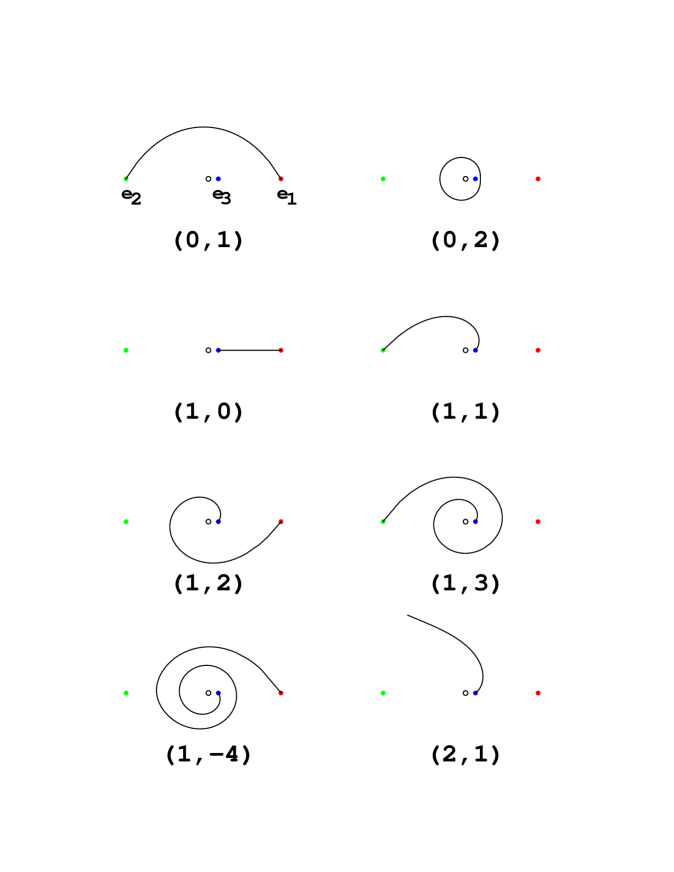
  Figure 1: $N_{f}=1$ , $u=-1$ , $m=0$

  In this picture we have depicted the results of our analysis. Stable states correspond to closed trajectories or open trajectories running between two branchpoints. Trajectories that run off to infinity or to zero correspond to unstable states. The string representing e.g. the monopole goes from the branchpoint $e_{1}$ to $e_{3}$. These are the branchpoints which collapse at the singularity $u=u_{1}$. On the CYM this then corresponds to a vanishing three–cycle around which the three–brane is wrapped. All dyons $\pm(1,n)$ and $\pm(1,2n^{\prime})$ are present in agreement with table (1.6). The other two states, becoming massless at $u_{2}$ and $u_{3}$ show up in a very similar way. The gauge boson is represented by a closed (counterclockwise) geodesic around the branchpoints $e_{3}$ and the point $z=0$ which is drawn as a small circle in our pictures. Thus we find the expected weak coupling spectrum. The trajectory for the $(2,1)$ state runs to infinity i.e. this state is unstable.

• $u=-1,\ \ m=0.5$:

  

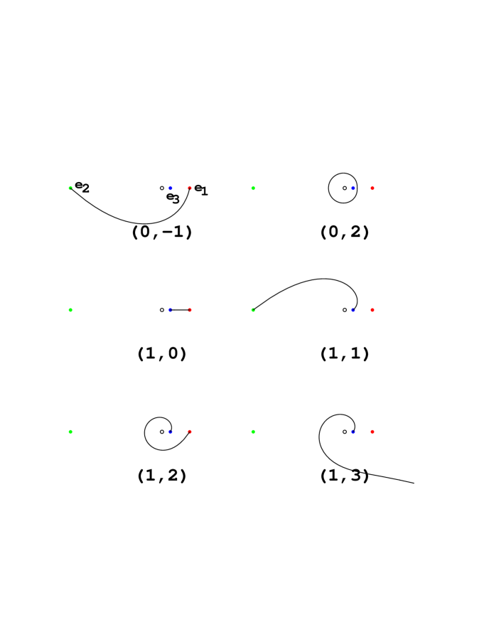
  Figure 2: $N_{f}=1$ , $u=-1$ , $m=0.5$

  In the massive case we encounter a residue of $\frac{2m}{2\pi i}$ at $z=\infty$. A residuum has the effect that the periods $a$ and $a_{D}$ are no longer invariant when we deform the homology cycles across $z_{R}$. Therefore, it modiefies the BPS mass formula and the equation for the geodesics. On the other hand, this fact is important to guarantee the existence of the strings $(1,0),(1,1)$ and $(1,2)$ which are responsible for the singularities at $u_{1}(m),u_{2}(m)$ and $u_{3}(m)$, respectively, for non–vanishing masses. This is also precisley what we see in the picture and without this modification, we would not obtain e.g.: the dyon $(1,1)$. We also see that already some dyons with odd electric charge $(1,2n+1)$ disappear from the spectrum, i.e. in the string picture their geodesics run to zero or infinite. We studied the spectra for various real values of $m$ and found that for increasing $m$ more and more $(1,2n+1)$ dyons disappear. Only the $(1,1)$ dyon is present also for large mass. E.g.: the $(1,3)$ dyon is still present for $m=0.1$, but no longer in fig. 2 at $m=0.5$

  Recently, in [34] some arguments were given, that $S$ is also a function of $u$ and differs from its value in the massless case. The quark $S=1$ has period $a+m$ but in our picture the state $(1,0)$ has period $a_{D}$ and not $a_{D}+m/2$ which one would expect from the mass formula for the monopole with $S=1/2$. Similarly the periods for the $(1,2n)$ dyons is $a_{D}+2na$. On the other hand for the $(1,1)$ state with $S=-1/2$ the period is $a_{D}+a-m$ and not $a_{D}+a-m/2$. For the other states with odd electric charge the period is $a_{D}+(2n+1)a-m$. Thus it seems that part of the contribution of the residue is already included in $a_{D}$. This means that as we send $m$ to infinity the monopole and the dyons with even electric charge survive since $a_{D}$ and $a$ remain finite in this limit but the $(1,1)$ dyon disappears because its mass becomes infinite. The difference of the $S$ quantum numbers is the same in the massive and the massless case but the absolute value changes in the massive case. This supports the conclusion that the quark number $S$ has to be distinguished from its physical value that appears in the central charge formula [34].

• $m\rightarrow\infty$ , $\Lambda_{1}\rightarrow 0$:

  As we increase the mass, we should finally end up with SYM with the matterfield being effectively integrated out. From the curve (3.11) written in the form:

  $$W=\Lambda_{0}^{2}\left[\frac{1}{\tilde{z}}+4\tilde{u}+4\tilde{z}+\tilde{z}^{2}\frac{\Lambda_{0}^{2}}{m^{2}}\right]-x^{2}\ ,$$ (3.15)

  with $\tilde{z}=z\sqrt{\frac{m}{\Lambda_{1}^{3}}}$ , $\tilde{u}=\frac{u}{\Lambda_{0}^{2}}$ and $m\Lambda_{1}^{3}=\Lambda_{0}^{4}$ we obtain from (3.12)

  $$\lambda_{SW}^{N_{f}=1}=2\Lambda_{0}\frac{d\tilde{z}}{\tilde{z}}\sqrt{\frac{1}{\tilde{z}}+4\tilde{u}+4\tilde{z}+\tilde{z}^{2}\frac{\Lambda_{0}^{2}}{m^{2}}}\ .$$ (3.16)

  From these expressions one recovers how pure SYM arises for $m\rightarrow\infty$. For the limit $m\rightarrow\infty$ we obtain the $W$ and $\lambda$ of [20] up to irrelevant rescalings which do not change the $J$–function. Whereas $\tilde{e}_{1}=e_{1}\sqrt{\frac{m}{\Lambda_{0}^{2}}}$ and $\tilde{e}_{3}$ become the branchpoints of the SW–curve, expressed in $\tilde{u}$, namely

  $$\tilde{e}_{1,3}\longrightarrow-\frac{\tilde{u}}{2}\pm\frac{1}{2}\sqrt{\tilde{u}^{2}-\Lambda_{0}^{4}}\ ,$$ (3.17)

  the third branchpoint $\tilde{e}_{2}$ moves to infinity:

  $$e_{2}\longrightarrow-\infty\ .$$ (3.18)

  During that process we loose many stable BPS states, namely all $(1,2n+1)$–dyons, which end at $e_{2}$ and become heavy. The three singularities $u_{1}(m),u_{2}(m)$ and $u_{3}(m)$ become

  $$\begin{array}[]{lcl}\tilde{u}_{1,3}&\longrightarrow&\pm 1\vspace{.2cm}\\ u_{2}&\longrightarrow&m^{2}\vspace{.2cm}\\ \end{array}$$

  in agreement with what one expects [4]. In particular this means that the quark becomes massless in the weak–coupling region at $u\rightarrow u_{2}(m)=m^{2}$.

  Looking at fig.1, at this limit $e_{2}\longrightarrow e_{3}$ and one would expect the dyon (1,1) to become massless at this point. However, as noted in [4] there is an interesting phenomenon happening when we increase the mass from zero to higher values. What appears as a dyon for small mass appears as an elementary particle for large mass. This is due the non-Abelian monodromies since what we call a monopole depends on the choice of a basepoint and a path around the singularity in the moduli space. When we start to increase the mass the singularities will move around each other in moduli space and the chosen path is deformed and will differ from the natural choice of path we would make for large mass. When we change the choice of paths the monodromy will be conjugated while it still belongs to same conjugacy class. This conjugation changes the magnetic and electric quantum numbers e.g. a dyon may become a quark.

• $u=0,\ \ m=0$:

  

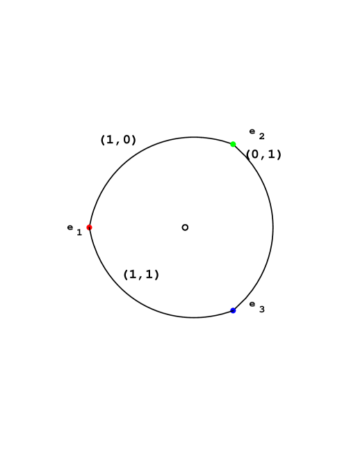
  Figure 3: $N_{f}=1$ , $u=0$ , $m=0$

  Notify that the dyon $(1,2)$ shows up with the quantum numbers $(0,1)$ in the strong coupling region. This is because, in general, one has to relabel quantum numbers when crossing a branch cut of the periods to guarantee the BPS mass formlua (1.2) to stay a smooth function in $u$ [11]. In other words, these states are related to the conventional notation of the strong–coupling states $\{(1,0),(1,1),(1,2)\}$, which only refer to a certain choice of paths around the singularities and a choice of the basepoint. For the basepoint $u=0$ the path for the $(1,2)$ state is not the natural choice. The natural path around $u_{3}$ yields a dyon with charges $(0,1)$ and the corresponding monodromy is related to the monodromy of the $(1,2)$ state by conjugation. It is the quantum number $S$ which says that this state with electric charge one is rather a dyon $(S=\frac{1}{2}$) than a quark ($S=1$). In this picture we also see very nicely the appearance of a monopole and two dyons with mutually non–local charges ‘at the same time’, i.e their monodromies do not commute. As we have explained before, on the CYM these states correspond to three–cycles with non–trivial intersection number. At the curve of marginal stability the $W$–boson decays. This decay, involving an interaction between particles with mutually non–local charges, can be recognized in the picture: The sum of the paths of all three strings with magnetic charge adds up to a closed circle, which includes $e_{0}=0$. Therefore, after fig. (1) it must be identified with the $W$–boson.

  $$(0,2)=(1,1)+(0,1)-(1,0)\ .$$ (3.19)

  There is a minus–sign for the monopole, since this string goes into the opposite direction, in contrast to all other states which go counterclockwise, in agreement with the $W$–boson in fig. (1). Thus, we see that the $W$–boson appears ‘virtually’ in the figure. After multiplying eq. (3.19) by two we recover the $W$–boson decay which preserves the $S$–charge [11]

  $$(0,2)_{0}\longrightarrow 4(0,1)_{\frac{1}{2}}+2(1,-1)_{-\frac{1}{2}}+2(-1,0)_{-\frac{1}{2}}\ .$$ (3.20)

• $u=0.3,\ \ m=0.5$:

  

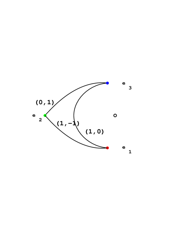
  Figure 4: $N_{f}=1$ , $u=0.3$ , $m=0.5$

  In the massive case, we keep all three strong–coupling states, since we still have the three singularities in the $u$–plane, which have moved depending on the mass $m$. This is in agreement with table (1.7). We are now in a strong–coupling region where it is not possible to obtain formally the $W$–boson loop surrounding $e_{0}$. We have:

  $$(0,1)+(1,-1)-(1,0)=(0,0)\ .$$ (3.21)

  Notify, that we have really zero on the right hand side, since we also do not encounter the residuum.

• $u=0,\ \ m=0.75$:  
  In the $N_{f}=1$ case we have a superconformal point at e.g.: $u=\frac{3}{4}=m$, where two particles with mutually non–local charges become massless. In this case these are the dyons $(1,1)$ and $(1,2)$ [17, 13]. At such points all three branchpoints coincide, as it can already be seen from fig. (5). Since these two dyon–strings run between two such branchpoints, from the string–picture it is obvious that these particles become massless. Since one is able to approach this limit while keeping both states this could be a hint that string–theory may be the right framework to describe the physics near and at the superconformal points. The periods vanish at this point. After (1.2) this indicates that the mass of the other BPS states is entirely given by the residuum. As in fig. 3 we can visualize the $W$–boson:

  $$(0,2)=(-1,0)+(1,1)-(0,-1)\ ,$$ (3.22)

  allowing for the decay (3.20) with non–trivial interactions. Again, the sign of $(0,-1)$ is reversed, since it runs clockwise, in contrast to the other two dyons. In this case we also pick up a residuum, when encircling along the $W$–boson loop.

  

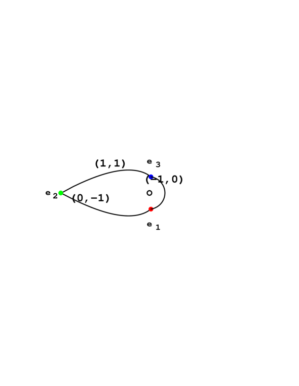
  Figure 5: $N_{f}=1$ , $u=0$ , $m=0.75$

$N_{f}=2:$  
 
For the $N_{f}=1$ case we have studied trajectories in the cut $P^{1}$–base. They are to be related to curves on the Riemann surface $\Sigma$. Therefore we can also investigate the properties of the BPS–states on this surface directly.

Let us now discuss the case with two flavours by writing down the necessary ingredients to find the BPS–states. The details about the relevant CYM can be found in [27]. The curve one ends up is:

$$y^{2}=\left(x^{2}-\frac{\Lambda^{4}_{2}}{64}\right)(x-u)+\frac{m^{2}\Lambda_{2}^{2}x}{4}-\frac{m^{2}\Lambda_{2}^{4}}{32}\ ,$$ (3.23)

where we have set $m_{1}=m_{2}=m$. In the $x$–plane we have the following three branchpoints:

$$\begin{array}[]{lcl}e_{1}&=&\displaystyle{\frac{\Lambda_{2}^{2}}{8}\vspace{.2cm}}\\ e_{2}&=&\displaystyle{\frac{u}{2}-\frac{\Lambda_{2}^{2}}{16}-\frac{1}{16}\sqrt{(\Lambda_{2}^{2}-8u)^{2}-32\Lambda_{2}^{2}(2m^{2}-u)}\vspace{.2cm}}\\ \vspace{.2cm}\\ e_{3}&=&\displaystyle{\frac{u}{2}-\frac{\Lambda_{2}^{2}}{16}+\frac{1}{16}\sqrt{(\Lambda_{2}^{2}-8u)^{2}-32\Lambda_{2}^{2}(2m^{2}-u)}\ .}\end{array}$$

The positions of the three strong coupling singularities are:

$$\begin{array}[]{lcl}u_{1,2}&=&\displaystyle{-\frac{\Lambda_{2}^{2}}{8}\mp\Lambda_{2}m\vspace{.2cm}}\\ u_{3}&=&\displaystyle{\frac{\Lambda_{2}^{2}}{8}+m^{2}}\end{array}$$

The meromorphic one-form is given by:

$$\lambda^{N_{f}=2}_{SW}=-\frac{\sqrt{2}}{4\pi}\frac{dxy}{x^{2}-\frac{\Lambda_{2}^{4}}{64}}\ .$$ (3.24)

Notify that this one–form has a residue at $x_{R}=-\frac{1}{8}\Lambda_{2}^{2}$. For generic masses there is also a residue at $x_{R}=\frac{1}{8}\Lambda_{2}^{2}$ which vanishes when the masses are chosen to be equal. The residue vanishes for the limit $m\rightarrow\infty,\Lambda_{2}\rightarrow 0$ with $m^{2}\Lambda_{2}^{2}=\Lambda_{0}^{4}$, in agreement with the fact that we do not expect any residuum in the pure SYM case [4]. Let us first discuss the weak–coupling region:

• $u=1$,  $m=0$:

  

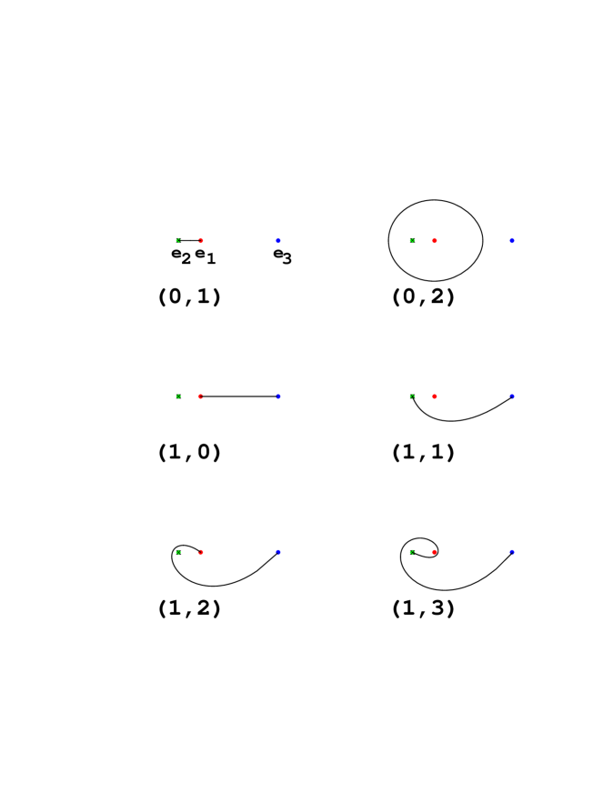
  Figure 6: $N_{f}=2$ , $u=1$ , $m=0$

  As in the $N_{f}=1$ case we find the expected weak-coupling spectrum (1.6); the quark and the dyons are represented by open trajectories and the W-boson by a closed one. The cross in the $N_{f}=2$ pictures denotes the branchpoint at $x=-\frac{1}{8}\Lambda_{2}^{2}$ which, in the case of non–zero mass $m$, coincides with the location of the residue. We were not able to find closed geodesics with magnetic quantum numbers greater than one and conclude that these states are unstable as expected.

• $u=1$,  $m=0.7$:

  

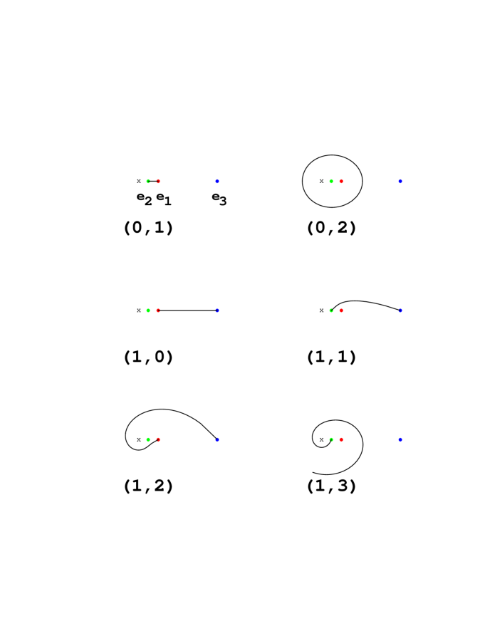
  Figure 7: $N_{f}=2$ , $u=1$ , $m=0.7$

  In the massive case the form of the periods for the BPS states is the same as in the $N_{f}=1$ case i.e. we have $a_{D}+2na$ for $(1,2n)$ dyons and $a_{D}+(2n+1)a+m$ for the $(1,2n+1)$ dyons. If we stay at weak coupling and turn on the mass, the higher the mass becomes, the more $(1,2n+1)$ dyons with large elecric charge disappear. In particular we see that the spectrum does not jump suddenly. Only the $(1,1)$ dyon fig. (7) survives also at large $m$ since it is responsible for the singularity at $u=u_{3}$. In the flow to the pure gauge theory this singularity goes to infinity and the singularities at $u=u_{1,2}$ become the monopole and dyon point of the pure SYM theory.

• $u=0$,  $m=0$:

  As we decrease $u$ for $m=0$ we will cross the curve of marginal stability where all states decay into two states, the monopole $(1,0)$ and the $(1,1)$ dyon.

  

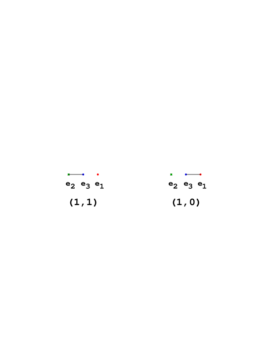
  Figure 8: $N_{f}=2$ , $u=0$ , $m=0$

  In our analysis the strong coupling spectrum appears as two straight open strings stretched between two branchpoints (with opposite direction). See fig. (8). Again, both states add up to the $W$–boson cycle

  $$(0,2)\longrightarrow 2(1,1)-2(1,0)\ ,$$ (3.25)

  after taking into account the different directions of the two strings.

• $u=0$,  $m=0.7$:

  

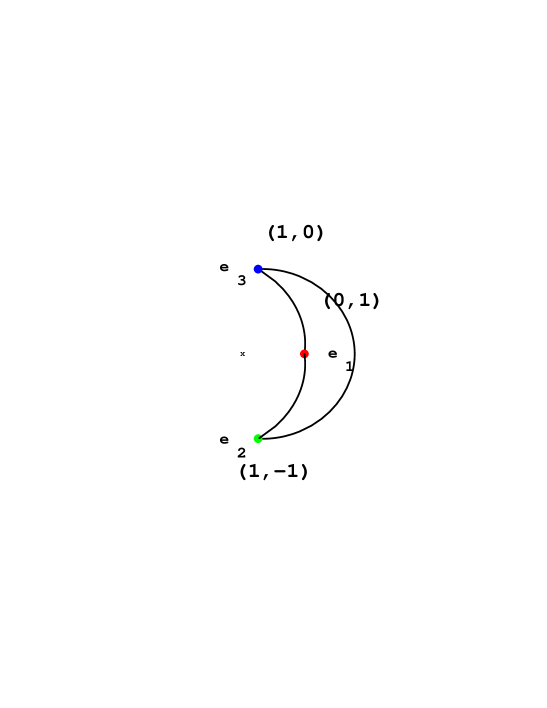
  Figure 9: $N_{f}=2$ , $u=0$ , $m=0.7$

  On the other hand, when we turn on the mass, the monopole singularity $u_{12}=-\frac{\Lambda_{2}^{2}}{8}$ splits into two singularities $u_{1,2}$ [cf. eq. (3.26)] and therefore we expect three dyonic states in the strong coupling regime [e.g.: $(1,0),\ (1,1),\ (1,2)$]. After fig. (9) these three states add up to zero, since we do not encounter the zero $e_{0}$ like the $W$–boson in fig. (7):

  $$(0,1)+(1,-1)-(1,0)=(0,0)\ .$$ (3.26)

  We also do not pick up a residuum. This picture is similar to fig. (4).

$N_{f}=3$:  
 
The curve for the theory with three flavors of equal mass is given by [4]:

$$W=x^{2}(x-u)-\frac{1}{64}\Lambda_{3}^{2}(x-u)^{2}-\frac{3}{64}m^{2}\Lambda_{3}^{2}(x-u)+\frac{1}{4}m^{3}\Lambda_{3}x-\frac{3}{64}m^{4}\Lambda_{3}^{2}\ .$$ (3.27)

The differential takes the following form:

$$\lambda_{SW}^{N_{f}=3}=\frac{\sqrt{2}}{8\pi}\frac{dx\ x(3m^{2}+6m^{3}-4mu+2mx-2ux+x^{2})}{(m^{2}-x^{2})\sqrt{-3m^{4}+3m^{2}-u^{2}-3m^{2}x+2m^{3}x+2ux-x^{2}-ux^{2}+x^{3}}}.$$ (3.28)

where we have set $\Lambda_{3}=8$. The three branchpoints are determined to ($m=0$)::

$$\begin{array}[]{lcl}e_{1}&=&u\vspace{.2cm}\\ e_{2}&=&\displaystyle{\frac{1}{2}(1+\sqrt{1-4u})\vspace{.2cm}}\\ e_{3}&=&\displaystyle{\frac{1}{2}(1-\sqrt{1-4u})\ .}\end{array}$$

They collapse $e_{1}\rightarrow e_{3}$ for $u\rightarrow 0$ with the monopole becoming massless and $e_{3}\rightarrow e_{2}$ for $u\rightarrow\frac{1}{4}$ with the $(2,-1)$ dyon becoming massless, respectively. Let us focus on two cases with zero mass, both at weak coupling. They differ by the arrangement of the branchpoints in the $x$–plane. From these two examples, one can see how different the BPS–states are represented depending on the modulus. E.g.: in fig. 10 one would guess the quark becoming massless for $e_{2}\rightarrow e_{3}=\frac{1}{2}$. However, in fig. 11, which is also the right patch to approach this limit, one realizes that when $e_{2},e_{3}\rightarrow\frac{1}{2}$ and $e_{1}\rightarrow\frac{1}{4}$ the quark encloses the branchpoint $e_{1}$, i.e. it cannot become massles.

• $u=-6$,  $m=0$:

  

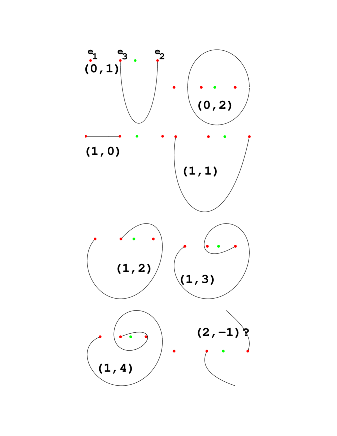
  Figure 10: $N_{f}=3$ , $u=-6$ , $m=0$

  In this case we have: $e_{1}=-6,\ e_{2}=3,\ e_{3}=-2$. The geodesics we found are the quark, the W-boson and the $(1,n)$ dyons in agreement with (1.6). But the strings corresponding to states with magnetic charge two predicted by [4] could not be found despite strong efforts fig.(10).

• $u=1/2$,  $m=0$:

  

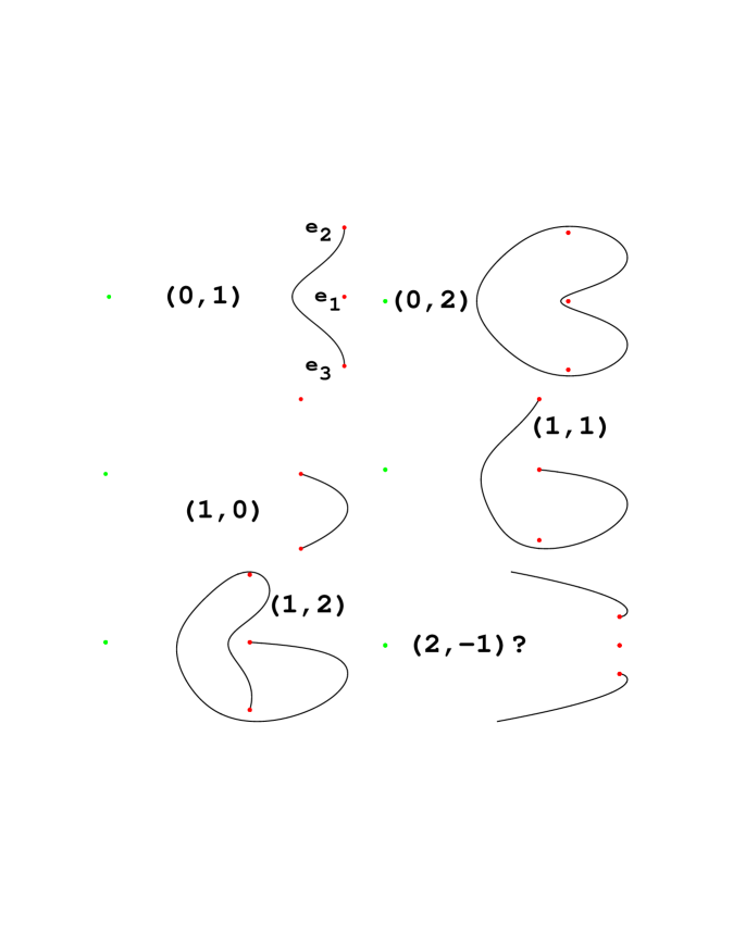
  Figure 11: $N_{f}=3$ , $u=\frac{1}{2}$ , $m=0$

The situation is similar to the $u=-6$ case, the states with magnetic charge up to one were found but in our pictures the $(2,-1)$ state has a non–expected behaviour: For the case of $u=1/2$, it should be represented by a geodesics starting at $e_{2}$, passing by $e_{1}$ and finally ending at $e_{3}$. This fact could be related that the meromorphic differential (3.28) is not the canonical one.

For the strong–coupling spectrum we obtain a similar figure as fig. 8 with $(1,1)$ just replaced by $(2,-1)$.

4 Concluding remarks

We have studied the spectrum and the stability of BPS states in N=2 SYM theory with $N_{f}=1,2,3$ massive flavours in the fundamental representation. This has been accomplished by investigating a point–particle limit of the underlying typeII string–compactifi–cation which leads to the corresponding $SU(2)$ SYM theory with massive matter. The BPS–states arise on typeIIB from three–branes in ten dimensions. After wrapping them around the vanishing two–cycles of the local $K3$ they become self–dual strings on an Riemann manifold $\Sigma$ which is equivalent to the SW–torus. We could establish a correspondence between self–dual strings on such manifolds and the field–theoretical BPS–states one expects from N=2 SYM. This enabled us to study their stability and strong–coupling behaviour. Indeed we could verify the tables, shown in the introduction, up to one discrepancy concerning the $(2,1)$ state in the $N_{f}=3$ case. In this picture gauge fields and monopoles appear on equal footing, since the two homology cycles of $\Sigma$ correspond to magnetically and electrically charged self–dual strings, respectively. This picture seems to be the right framework to describe, e.g. particles with mutually non–local charges becoming massless or decaying at certain regions in the moduli space. This is a quite difficult task in field theory where gauge bosons appear as elementary particles and monopoles as solitonic solutions or vice versa.

Unfortunately, for the case of three flavours we could not find evidence for the existence of the $(2,1)$ state, which would be very important for consistency which follows from matching the $m\rightarrow\infty$ spectrum with flavour symmetry $SU(3)\times U(1)$ (for equal quark masses) with the $m=0$ spectrum with $SU(4)$. We interpret [11] such that the existence of the dyon (2,1) was established on the ground of [7], mainly because of the lack of a ${\sf Z\kern-3.99994ptZ}$–symmetry in the moduli space. In global N=2 SUSY one can construct such a state [7]. But it still remains to proof that the curve for the $N_{f}=3$ case also allows for such a state as it has been proposed in [4].

The SW–geometries and their BPS–spectra arise in [19, 20] and for the cases, we considered here, from higher dimensional theories with extended objects, namely type IIB with solitonic three–branes. There are now many recent results where the curve or the effective action of N=2 SYM without or with massive matter emerges either as useful tool to describe some deformations away from an orbifold point of $F$–theory on $K3$ [35], as effective theories which describe some higher dimensional theories in a certain region of their moduli space [36] or as part of a more complicated theory [37, 38] and e.g. (1.2) arises as the mass of $(p,q)$–strings going between different branes [39]. Therefore it should be possible to obtain the results we have gotten here within those frameworks. I.e. starting from the BPS–states in these theories one should be able to deduce constraints for the field–theortical Seiberg–Witten spectrum. This was done partially in [39] based on the equivalence between N=2 $SU(2)$ SYM with $N_{f}=4$ and the world–volume theory of a three–brane of type IIB in the presence of a configuration of four 7 D–branes and an orientifold plane [38]. In this case, the mass formula of the BPS–states (1.2) can be related to the mass of an open string going from a three–brane to a seven–brane. A BPS state is obtained when the mass is minimized, i.e. when the path from the three–brane to the seven–brane goes along a geodesics. Notify, that ref. [36] obtains also the curves for $N_{f}=3$. Geodesics have also appeared recently in a different context, when discussing symmetry enhancement in $F$–theory on $K3$, where open strings representing the $W$–bosons connect seven–branes along geodesics [40].

$Acknowledgement:\$ We would like to thank W. Lerche and P. Mayr for drawing our attention to the problems presented here. Moreover, we are very grateful to J.–P. Derendinger, P. Mayr, A. Klemm, W. Lerche and S. Theisen for helpful discussions. We also thank J.–P. Derendinger for providing excellent working conditions in Neuchâtel and P. Béran for some Fortran assistance. The research of A. B. has been supported in part by the Bundesministerium für Wissenschaft, Verkehr und Kunst.

References

- [1]
- [2]
- [3] N. Seiberg and E. Witten, Nucl. Phys. B 426 (1994) 19
- [4] N. Seiberg and E. Witten, Nucl. Phys. B 431 (1994) 484
- [5] For a review see e.g.: W. Lerche, Notes on N=2 supersymmetric gauge theory, Proceedings Gauge Theories, Applied Supersymmetry and Quantum Gravity, pp. 53–79, Leuven University Press (1996)
- [6] A. Sen, Phys. Lett. B 329 (1994) 217
-
[7]
S. Sethi and M. Stern, hep–th/9507145;
S. Sethi, M. Stern and E. Zaslow, hep–th/9508117;
J.P. Gauntlett and J.A. Harvey, hep–th/9508156 - [8] A. Klemm, W. Lerche and S. Theisen, Int. J. Mod. Phys. A 11 (1996) 1929
-
[9]
A. Brandhuber and S. Stieberger, hep–th/9609130;
Y. Ohta, hep–th/9604051 and hep–th/9604059;
T. Masuda and H. Suzuki, hep–th/9609066, hep–th/9609065 - [10] K. Ito and S. Yang, Phys. Lett. B 366 (1996) 165
- [11] A. Bilal and F. Ferrari, hep–th/9605101
- [12] P.C. Argyres and M. Douglas, Nucl. Phys. B 448 (1995) 93
- [13] P.C. Argyres, M. Plesser, N. Seiberg and E. Witten, Nucl. Phys. B 461 (1996) 71
- [14] M. Matone Phys. Rev. D 53 (1996) 7354
- [15] M. Henningson, Nucl. Phys. B 461 (1996) 101
- [16] P. C. Argyres, A. Faraggi and A. Shapere, hep–th/9505190
- [17] F. Ferrari and A. Bilal, Nucl. Phys. B 469 (1996) 387
-
[18]
W. Lerche, D.-J. Smit and N.P. Warner, Nucl. Phys. B 372 (1992) 87;
A. Klemm, B.H. Lian, S.S. Roan and S.T. Yau, hep–th/9407192 - [19] S. Kachru, A. Klemm, W. Lerche, P. Mayr and C. Vafa, Nucl. Phys. B 459 (1996) 537
- [20] A. Klemm, W. Lerche, P. Mayr, C. Vafa and N. Warner, hep–th/9604034
- [21] S. Kachru and C. Vafa, Nucl. Phys. B 450 (1995) 69, hep-th/9505105
- [22] A. Klemm, W. Lerche and P. Mayr, Phys. Lett. B 357 (1995) 313
- [23] P. Aspinwall and J. Louis, Phys. Lett. B 369 (1996) 233
-
[24]
C.M. Hull and P.K. Townsend, Nucl. Phys. B 438 (1995) 109;
E. Witten, Nucl. Phys. B 443 (1995) 85 - [25] W. Lerche and N.P. Warner, hep–th/9608183
- [26] E. Martinec and N. Warner, Nucl. Phys. B 459 (1996) 97, hep-th/9509161
- [27] W. Lerche, P. Mayr and N. Warner, to appear
- [28] E. Witten, hep–th/9507121
- [29] M. Bershadsky, C. Vafa and V. Sadov, hep–th/9510225
- [30] A. Strominger, Nucl. Phys. B 451 (1995) 96
- [31] K. Landsteiner, E. Lopez and D. A. Lowe, hep–th/9606146
- [32] M. Porrati, hep–th/9607082, to appear in Phys. Lett. B
-
[33]
M. Porrati, Phys. Lett. B 377 (1996) 67;
G. Segal and A. Selby, Comm. Math. Phys. 177 (1996) 775 - [34] F. Ferrari, hep–th/9609101
- [35] A. Sen, hep–th/9605150
- [36] O.J. Ganor, hep–th/9608109
- [37] M. Douglas and M. Li, hep–th/9604041
- [38] T. Banks, M. Douglas and N. Seiberg, hep–th/9605199
- [39] A. Sen, hep–th/9608005
- [40] A. Johansen, hep–th/9608186