UKC/IMS/96-52
Cyclic Monopoles

Abstract

We study charge $k$ $SU(2)$ BPS monopoles which are symmetric under the cyclic group of order $k$. Approximate twistor data (spectral curves and Nahm data) is constructed using a new technique based upon a Painlev’e analysis of Nahm’s equation around a pole. With this data both analytical and numerical approximate ADHMN constructions are performed to study the zeros of the Higgs field and the monopole energy densities. The results describe, via the moduli space approximation, a novel type of low energy $k$ monopole scattering.

1 Introduction

By studying rational maps it has been shown [5] that the imposition of cyclic $C_{k}$ symmetry upon strongly centred charge $k$ $SU(2)$ BPS monopoles selects out from the general $k$-monopole moduli space ${\cal M}_{k}$ a set of $k$ 2-dimensional totally geodesic submanifolds. Each of these 2-dimensional submanifolds is a surface of revolution, hence by application of a reflection symmetry a number of geodesics in ${\cal M}_{k}$ are obtained. In the moduli space approximation [9] these geodesics may be interpreted in terms of the motion of $k$ slowly moving monopoles. It is therefore of considerable interest to know more about these one-parameter families of monopoles. The rational map approach is limited for this purpose, and the only additional information it supplies concerns the asymptotic in and out states for the scattering process.

Other twistor approaches yield more information about the monopole, but are more difficult to apply than the rational map method. In [5] only the form of the corresponding spectral curves was found. In this paper we do a little better, by constructing approximate spectral curves, which of course have this required form. Moreover, we construct approximate Nahm data and implement an ADHMN construction to compute the Higgs field and energy density of these monopoles.

The technique used is to make use of the integrability of Nahm’s equation, not to attempt an explicit solution, but rather to study the nature of a solution around a given pole, with the aid of a little Painlev’e analysis. The method applies equally well to all values of $k$, but only the cases $k=3$ and $k=4$ will be discussed in detail.

2 Monopoles and ADHMN

$SU(2)$ BPS monopoles are topological soliton solutions of a Yang-Mills-Higgs gauge theory with no Higgs self-coupling. Boundary conditions imply that the Higgs field at infinity defines a map between two-spheres. This map has an integer valued winding number $k$, which we identity as the magnetic charge or number of monopoles. In this paper we shall be concerned with strongly centred monopoles, which basically means that we fix the centre of mass of the monopole configuration to be the origin, and set a total phase to be unity. For more precise details of strong centring and other background information on monopoles we refer the reader to [5, 2].

As mentioned in the introduction, requiring invariance of a $k$-monopole under cyclic $C_{k}$ symmetry, and an additional reflection symmetry, leads to a number of geodesics $\Sigma_{k}^{l}$ (we follow the notation of [5]) in the $k$-monopole moduli space ${\cal M}_{k}$. Essentially there are $(2k+3+(-1)^{k})/4$ different types of these cyclic geodesics, corresponding to $l=0,1,..k/2$ if $k$ is even and $l=0,1,..(k-1)/2$ if $k$ is odd. Physically, for $l\neq 0$, the associated monopole scatterings are distinguished by having the out state (or in state by time reversal) consisting of two clusters of monopoles with charges $k-l$ and $l$. This explains why we do not allow $l>k/2$, since this is basically the same scattering event as one of the geodesics with $l<k/2$. If $l=0$ then the monopoles remain in a plane and scatter instantaneously through the axisymmetric $k$-monopole and emerge with a $\pi/k$ rotation. This kind of $\pi/k$ scattering is essentially a two-dimensional process and has been extensively studied in planar systems [8]. In this paper we shall be concerned with the more exotic scatterings with $l\neq 0$. It should also be pointed out that the case $k=2$ is special, in that the geodesics $\Sigma_{2}^{0}$ and $\Sigma_{2}^{1}$ are isomorphic, so that there is only one type of scattering; the famous right-angle scattering found by Atiyah and Hitchin [2].

In this paper we shall only deal with the cases $k=3$ and $k=4$. The method applies equally well to all values of $k$, but all the important features are captured by these two examples. From the above we see that for $k=3$ there is only one interesting geodesic $\Sigma_{3}^{1}$. It describes three individual monopoles which scatter and emerge as a single monopole and a 2-monopole cluster. It also contains the tetrahedral 3-monopole [5, 6] as an instantaneous configuration. For $k=4$ there are two interesting geodesics $\Sigma_{4}^{2}$ and $\Sigma_{4}^{1}$. The first describes a scattering in which the monopoles emerge as two 2-monopole clusters, and also includes the cubic 4-monopole [5, 6]. The second describes a scattering which results in the formation of a single monopole and a 3-monopole cluster; no monopoles with the symmetries of a Platonic solid are contained in this geodesic.

There are several twistor techniques which are applicable to monopoles, but here our main tool will be the ADHMN [10, 4] construction. This is an equivalence between $k$-monopoles and Nahm data $(T_{1},T_{2},T_{3})$, which are three $k\times k$ matrices which depend on a real parameter $s\in[0,2]$ and satisfy the following;

(i) Nahm’s equation

$$\frac{dT_{i}}{ds}=\frac{1}{2}\epsilon_{ijk}[T_{j},T_{k}]$$

(ii) $T_{i}(s)$ is regular for $s\in(0,2)$ and has simple poles at $s=0$ and $s=2$,

(iii) the matrix residues of $(T_{1},T_{2},T_{3})$ at each pole form the irreducible $k$-dimensional representation of SU(2),

(iv) $T_{i}(s)=-T_{i}^{\dagger}(s)$,

(v) $T_{i}(s)=T_{i}^{t}(2-s)$.

Equation (i) is equivalent to a Lax pair and hence there is an associated algebraic curve, which is in fact the spectral curve [4]. Explicitly, the spectral curve may be read off from the Nahm data as the equation

$$\mbox{det}(\eta+(T_{1}+iT_{2})-2iT_{3}\zeta+(T_{1}-iT_{2})\zeta^{2})=0.$$ (2.1)

It is useful to construct the spectral curve since it not only gives a convenient representation of the monopole, but also furnishes the constants for Nahm’s equation.

The procedure by which the Higgs field (and gauge potential) can be reconstructed from the Nahm data is outlined in section 5, where our analytical approximation to this procedure is also discussed.

In the next section we give the general form for cyclic $k$-monopole Nahm data and introduce the relevant equations for the case $k=3$.

3 Cyclic Nahm data

As explained in [13] the form of the Nahm data for $C_{k}$ symmetric $k$-monopoles may be obtained as a linear sum of generators of the affine Lie algebra $A_{k-1}^{(1)}$. Explicitly, consider the Lie algebra $A_{k-1}^{(1)}$, with $H_{i}$, $i=0,..,k-1$ the generators of the extended Cartan subalgebra and $E_{\pm i}$ the generators corresponding to the simple roots $\alpha_{i}$, $i=1,..,k-1$, plus the lowest root $\alpha_{0}=-\sum_{j=1}^{k-1}\alpha_{j}$. In the Chevalley basis these satisfy

$$[H_{i},E_{\pm j}] =\pm C_{ij}E_{\pm j}$$ (3.1)

$$[E_{i},E_{-j}] =\delta_{ij}H_{j}$$ (3.2)

where $C_{ij}$ are the elements of the $k\times k$ extended Cartan matrix given by

$$C_{ij}=\frac{2(\alpha_{i},\alpha_{j})}{(\alpha_{i},\alpha_{i})},\hskip 28.45274pti,j=0,..,k-1.$$ (3.3)

Cyclic Nahm data may be expressed in terms of a linear sum of generators as

$$T_{1}-iT_{2}=\sum_{j=0}^{k-1}Q_{j}E_{+j},\hskip 28.45274ptT_{3}=i\sum_{j=0}^{k-1}P_{j}H_{j}$$ (3.4)

with real function coefficients $P_{j},Q_{j}$.

For the case $k=3$ a change of notation yields the Nahm data for $C_{3}$ symmetric 3-monopoles to have the form

$$T_{1}=\frac{1}{2}\left[\begin{array}[]{ccc}0&-f_{3}&f_{2}\\ f_{3}&0&-f_{1}\\ -f_{2}&f_{1}&0\end{array}\right];\ T_{2}=-\frac{i}{2}\left[\begin{array}[]{ccc}0&f_{3}&f_{2}\\ f_{3}&0&f_{1}\\ f_{2}&f_{1}&0\end{array}\right];\$$

$$T_{3}=i\left[\begin{array}[]{ccc}f_{4}&0&0\\ 0&f_{5}&0\\ 0&0&-(f_{4}+f_{5})\end{array}\right]$$ (3.5)

with corresponding spectral curve

$$\eta^{3}+\alpha\eta\zeta^{2}+\gamma\zeta^{3}+i\beta(\zeta^{6}+1)=0.$$ (3.6)

The constants $\alpha$, $\beta$, $\gamma$ can all be taken to be real, by imposition of a reflection symmetry, and are given in terms of the $f_{i}$’s as

$$\alpha= f_{1}^{2}+f_{2}^{2}+f_{3}^{3}-4(f_{4}^{2}+f_{5}^{2}+f_{4}f_{5})$$ (3.7)

$$\beta= -f_{1}f_{2}f_{3}$$

$$\gamma= 2f_{1}^{2}f_{4}+2f_{2}^{2}f_{5}-2(f_{3}^{2}+4f_{4}f_{5})(f_{4}+f_{5}).$$

For this data Nahm’s equation becomes

$$\dot{f}_{1}= (2f_{5}+f_{4})f_{1}$$ (3.8)

$$\dot{f}_{2}= -(2f_{4}+f_{5})f_{2}$$

$$\dot{f}_{3}= (f_{4}-f_{5})f_{3}$$

$$\dot{f}_{4}= (f_{3}^{2}-f_{2}^{2})/2$$

$$\dot{f}_{5}= (f_{1}^{2}-f_{3}^{2})/2.$$

The first calculation we require is to see how the tetrahedral 3-monopole sits inside this Nahm data. The spectral curve and Nahm data of the tetrahedral 3-monopole have been computed [5] for the monopole in a different orientation and it is possible to derive the answer we require by rotation of this known data. However, this is a non-trivial exercise which in fact requires more work than simply solving the equations again. Thus in the remainder of this section we compute the Nahm data and spectral curve of the tetrahedral 3-monopole in the orientation in which it has $C_{3}$ symmetry around the $x_{3}$ axis.

For tetrahedral symmetry we must have that $\alpha=0$, which is achieved by the following choice

$$f_{1}^{2}=2f_{4}^{2},\hskip 28.45274ptf_{2}^{2}=2f_{5}^{2},\hskip 28.45274ptf_{3}^{2}=2(f_{4}+f_{5})^{2}.$$ (3.9)

The remaining constants then simplify to

$$\gamma=-20f_{4}f_{5}(f_{4}+f_{5}),\hskip 28.45274pt\mbox{and}\hskip 28.45274pt\beta=-\frac{\gamma}{5\sqrt{2}}.$$ (3.10)

Using the above constants we can solve for $f_{5}$ in terms of $f_{4}$ as

$$2f_{5}=-f_{4}\pm\sqrt{f_{4}^{2}-\gamma/(5f_{4})}$$ (3.11)

and substituting this into the equation (3.8) for $f_{4}$ yields

$$\dot{f}_{4}^{2}=f_{4}(f_{4}^{3}-\gamma/5).$$ (3.12)

Introducing the variable $2w=-1/f_{4}$ this equation becomes the standard form elliptic equation

$$4\dot{w}^{2}=cw^{3}+1,\hskip 28.45274ptc=8\gamma/5.$$ (3.13)

Set

$$w=\wp(t)/(4\kappa)$$ (3.14)

with $t=\kappa s+B$ then, choosing $4\kappa=c^{1/3}$, $\wp$ is the Weierstrass elliptic function satisfying

$$\wp^{\prime 2}=4\wp^{3}+4$$ (3.15)

where prime denotes differentiation with respect to the argument. The real period of this elliptic function is

$$2\omega_{1}=\Gamma(1/6)\Gamma(1/3)/(2\sqrt{\pi}).$$ (3.16)

For the correct boundary conditions take the elliptic function to go between zeros at $t=2\omega_{1}/3$ and $t=4\omega_{1}/3$. This requires that $\kappa=\omega_{1}/3$ and $B=2\omega_{1}/3$. Now

$$-\beta=\frac{\gamma}{5\sqrt{2}}=\frac{c}{8\sqrt{2}}=\frac{(4\kappa)^{3}}{8\sqrt{2}}=\Gamma(1/6)^{3}\Gamma(1/3)^{3}/(\pi^{3/2}3^{3}8\sqrt{2}).$$ (3.17)

Thus we have arrived at the spectral curve

$$\eta^{3}-i(\zeta^{6}+i5\sqrt{2}\zeta^{3}+1)\Gamma(1/6)^{3}\Gamma(1/3)^{3}/(\pi^{3/2}3^{3}8\sqrt{2})=0.$$ (3.18)

It is a simple, though tedious, calculation to verify that this is indeed the spectral curve obtained by rotating the one given in [5].

We have yet to examine the residue behaviour of the functions, and this will be of vital importance in what follows later. For $t\sim B$

$$\wp(t-B)\sim-2(t-B)$$ (3.19)

and

$$f_{4}=-\frac{1}{2w}\sim\frac{4\kappa}{4(t-B)}=1/s.$$ (3.20)

The other relations then give $f_{5}\sim-1/s$, and hence

$$T_{3}\sim s^{-1}i\mbox{diag}(1,-1,0)$$

which identifies the representation formed by the residues as the irreducible one. As it will be needed later we list here the residue behaviour of all the functions at both ends of the interval,

$$f_{1}\sim\sqrt{2}/s,\ f_{2}\sim\sqrt{2}/s,\ f_{3}\sim 0/s,\ f_{4}\sim 1/s,\ f_{5}\sim-1/s,\hskip 28.45274pt\mbox{as}\ s\rightarrow 0$$ (3.21)

and defining the variable $\widetilde{s}=2-s$ then

$$f_{1}\sim\sqrt{2}/\widetilde{s},\ f_{2}\sim\ 0/\widetilde{s},\ f_{3}\sim\sqrt{2}/\widetilde{s},\ f_{4}\sim 1/\widetilde{s},\ f_{5}\sim 0/\widetilde{s},\hskip 28.45274pt\mbox{as}\ s\rightarrow 2.$$ (3.22)

4 Approximate twistor data

In principle the equations were are concerned with for cyclic $k$-monopoles are solvable in terms of abelian integrals of genus $(k-1)$ [13]. However, for $k>2$, to explicitly extract from the general solution the one which satisfies all the required boundary conditions appears to be a highly non-trivial exercise. Furthermore, one of the main motivations for constructing the Nahm data is so that it can be used as input in the numerical ADHMN algorithm [6], to provide a visualization of the monopole energy densities. Even if the required explicit solution could be determined it is by no means clear that it would be in a form suitable for obtaining numerical values; there are at present no numerical algorithms available to compute the Riemann theta function for a surface of genus greater than one, unless it happens to be of a very special form which allows Weierstrass reduction theory to be applied [3]. With this in mind we construct, in this section, approximate twistor data (ie. Nahm data and spectral curves) for $C_{3}$ symmetric 3-monopoles.

One of the key points in applying the following method is that we know explicitly the twistor data for one member of the family ie. the tetrahedral 3-monopole. The one parameter family of monopoles we are searching for is a geodesic in the monopole moduli space and it is known [11] that the transformation between the monopole moduli space metric and the metric on Nahm data is an isometry. Since the Nahm data has poles it follows from these two facts that the residues at these poles must be constant with respect to the geodesic parameter. The upshot is that we know the residue behaviour explicitly for all members of the one-parameter family, it is given by (3.21) and (3.22).

As equations (3.8) are integrable they possess a particular solution which is a single-valued expansion around the $s=0$ pole ie

$$f_{i}=\sum_{j=-1}^{\infty}a_{i,j}s^{j}$$ (4.1)

where the pole coefficients are given by (3.21) as

$$a_{1,-1}=\sqrt{2},\hskip 28.45274pta_{2,-1}=\sqrt{2},\hskip 28.45274pta_{3,-1}=0,\hskip 28.45274pta_{4,-1}=1,\hskip 28.45274pta_{5,-1}=-1.$$ (4.2)

We now need to determine the number of arbitrary constants in the above particular solution. This can be done using Painlev’e analysis [1, 14] as follows. We consider the two term expansion

$$f_{i}=\frac{a_{i,-1}}{s}+b_{i}s^{r-1}$$ (4.3)

for $r$ an arbitrary integer, and linearise the equation (3.8) to obtain

$$\left[\begin{array}[]{ccccc}r&0&0&-\sqrt{2}&-2\sqrt{2}\\ 0&r&0&2\sqrt{2}&\sqrt{2}\\ 0&0&r-3&0&0\\ 0&\sqrt{2}&0&r-1&0\\ -\sqrt{2}&0&0&0&r-1\end{array}\right]\left[\begin{array}[]{c}b_{1}\\ b_{2}\\ b_{3}\\ b_{4}\\ b_{5}\end{array}\right]=\left[\begin{array}[]{c}0\\ 0\\ 0\\ 0\\ 0\end{array}\right].$$ (4.4)

The Kowalevski exponents (they are not strictly resonances since $a_{3,-1}=0$) are determined by the vanishing of the determinant $\Delta$ of the above matrix. We have that

$$\Delta=(r-3)^{2}(r-2)(r+1)(r+2)$$ (4.5)

so there are three arbitrary constants in our particular solution, corresponding to the three (counted with multiplicity) positive roots of $\Delta$. Furthermore, we see that one of the arbitrary constants appears at the linear level in the $s$ expansion and the remaining two at quadratic level. Explicit calculation reveals that these may be taken to be $a_{1,1},a_{1,2}$ and $a_{3,2}$. We obtain that, to cubic order in $s$,

$$f_{1}= \sqrt{2}/s+a_{1,1}s+a_{1,2}s^{2}+\frac{7\sqrt{2}}{20}a_{1,1}^{2}s^{3}$$ (4.6)

$$f_{2}= \sqrt{2}/s+a_{1,1}s-a_{1,2}s^{2}+\frac{7\sqrt{2}}{20}a_{1,1}^{2}s^{3}$$

$$f_{3}= a_{3,2}s^{2}$$

$$f_{4}= 1/s-\sqrt{2}a_{1,1}s+\frac{1}{\sqrt{2}}a_{1,2}s^{2}-\frac{2}{5}a_{1,1}^{2}s^{3}$$

$$f_{5}= -1/s+\sqrt{2}a_{1,1}s+\frac{1}{\sqrt{2}}a_{1,2}s^{2}+\frac{2}{5}a_{1,1}^{2}s^{3}.$$

This is going to be the form of the functions in our approximate Nahm data. Note that we terminate the expansion at $O(s^{3})$, as this will turn out to be sufficient for our needs, but it is a simple matter to improve the accuracy of the approximate data by keeping higher order terms in the above.

At this stage we have a candidate three-parameter family of approximate data, from which we need to select the correct one-parameter family. The constraining conditions arise from consideration of a symmetry of the equations (3.8). As before, let $\widetilde{s}=2-s$, then if $f_{i}(s)$ is a solution we can construct a second solution $g_{i}(s)$ as

$$[g_{1}(s),g_{2}(s),g_{3}(s),g_{4}(s),g_{5}(s)]=[f_{1}(\widetilde{s}),f_{3}(\widetilde{s}),f_{2}(\widetilde{s}),f_{4}(\widetilde{s}),-f_{4}(\widetilde{s})-f_{5}(\widetilde{s})].$$ (4.7)

Note that if $f_{i}(s)$ is a solution of the form (4.6) with a pole at $s=0$ then $g_{i}(s)$ will have a pole at $s=2$. Furthermore, the residues at this pole will be precisely those of (3.22) which we require. Thus, we take our approximate solution to be $f_{i}(s)$ for $s\in[0,1]$ and $g_{i}(s)$ for $s\in[1,2]$. There is now the matching condition at $s=1$ that $g_{i}(1)=f_{i}(1)$, for $i=1,..,5$. The first and fourth of these equations are identities, while the second and third are equivalent, so we are left with the two matching conditions

$$f_{2}(1)=f_{3}(1)\hskip 28.45274pt\mbox{and}\hskip 28.45274ptf_{4}(1)=-2f_{5}(1).$$ (4.8)

These give two relations between the three parameters $a_{1,1},a_{1,2},a_{3,2}$ and thus determine the sought after one-parameter family. Using the series (4.6) the matching conditions give that

$$a_{3,2}= \sqrt{2}+a_{1,1}-a_{1,2}+\frac{7\sqrt{2}}{20}a_{1,1}^{2}$$ (4.9)

$$a_{1,2}= \frac{\sqrt{2}}{3}(1-\sqrt{2}a_{1,1}-\frac{2}{5}a_{1,1}^{2})$$

so that everything is determined by the parameter $a_{1,1}$ which we now relabel as $a$. In detail the functions are

$$f_{1}= \sqrt{2}/s+as+\frac{\sqrt{2}}{3}(1-\sqrt{2}a-\frac{2}{5}a^{2})s^{2}+\frac{7\sqrt{2}}{20}a^{2}s^{3}$$ (4.10)

$$f_{2}= \sqrt{2}/s+as-\frac{\sqrt{2}}{3}(1-\sqrt{2}a-\frac{2}{5}a^{2})s^{2}+\frac{7\sqrt{2}}{20}a^{2}s^{3}$$

$$f_{3}= (\sqrt{2}+a-\frac{\sqrt{2}}{3}(1-\sqrt{2}a-\frac{2}{5}a^{2})+\frac{7\sqrt{2}}{20}a^{2})s^{2}$$

$$f_{4}= 1/s+\sqrt{2}as+\frac{1}{3}(1-\sqrt{2}a-\frac{2}{5}a^{2})s^{2}-\frac{2}{5}a^{2}s^{3}$$

$$f_{5}= -1/s-\sqrt{2}as+\frac{1}{3}(1-\sqrt{2}a-\frac{2}{5}a^{2})s^{2}+\frac{2}{5}a^{2}s^{3}.$$

The next item to consider is the expression for the ‘constants’, $\alpha,\beta$ and $\gamma$. Of course they are only constant for exact solutions of the equations so for our approximate solutions (4.10) they will have higher order corrections in $s$. Explicitly we find that $\alpha=\alpha_{0}+O(s^{4})$, $\beta=\beta_{0}+O(s^{2})$ and $\gamma=\gamma_{0}+O(s^{2})$ where

$$\alpha_{0}= 12\sqrt{2}a$$ (4.11)

$$\beta_{0}= -\frac{1}{3}(4\sqrt{2}+10a+\frac{29\sqrt{2}}{10}a^{2})$$

$$\gamma_{0}= \frac{8}{3}(5-5\sqrt{2}a-2a^{2}).$$

The second piece of approximate twistor data is thus the family of approximate spectral curves

$$\eta^{3}+\alpha_{0}\eta\zeta^{2}+\gamma_{0}\zeta^{3}+i\beta_{0}(\zeta^{6}+1)=0.$$ (4.12)

It is useful to analyse these curves, as it gives an indication as to the accuracy of the approximate construction.

The first comparison that can be made is with the the exact tetrahedral 3-monopole spectral curve (3.18). This has

$$\alpha=0,\hskip 28.45274pt\gamma=-5\sqrt{2}\beta,\hskip 28.45274pt-\beta=\frac{\Gamma(1/6)^{3}\Gamma(1/3)^{3}}{\pi^{3/2}3^{3}8\sqrt{2}}\approx 1.95.$$ (4.13)

For the approximate curve to have $\alpha_{0}=0$ requires $a=0$, then by the above formulae we obtain

$$\alpha_{0}=0,\hskip 28.45274pt\gamma_{0}=-5\sqrt{2}\beta_{0},\hskip 28.45274pt-\beta_{0}=4\sqrt{2}/3\approx 1.89.$$ (4.14)

Note the surprising result that the relation between $\beta_{0}$ and $\gamma_{0}$ is exact in this case, so that the approximate spectral curve has tetrahedral symmetry. The value of $\beta_{0}$ is also very close to the true $\beta$ value, considering the low order approximation we chose. Clearly the accuracy of the approximate curves could be improved by performing an identical construction as above but taking a higher order approximating series.

By considering asymptotic spectral curves we shall now determine the range of the parameter $a$, and also make some further comparisons. The asymptotic monopole configurations along the exact geodesic can be determined from the corresponding rational map [5]. At one end the configuration is that of three well-separated unit charge monopoles on the vertices of a large equilateral triangle in the $x_{1}x_{2}$-plane. At the other end the configuration is asymptotic to an axisymmetric 2-monopole on the negative $x_{3}$-axis, with the $x_{3}$-axis the axis of symmetry, and a unit charge monopole on the positive $x_{3}$-axis. These two clusters are well-separated with the distance from the origin of the 1-monopole being twice that of the 2-monopole.

The spectral curve of a 1-monopole with position $(x_{1},x_{2},x_{3})$ is

$$\eta-(x_{1}+ix_{2})+2x_{3}\zeta+(x_{1}-ix_{2})\zeta^{2}=0$$ (4.15)

and is called a star. By taking a product of such stars the asymptotic spectral curves corresponding to the above configurations can be determined [5]. Taking three unit charge monopoles in the $x_{1}x_{2}$-plane with coordinates $x_{1}+ix_{2}=ib\omega^{j}$, $j=0,1,2$ and $\omega=e^{2\pi i/3}$ gives the product of stars

$$0=(\eta-ib(1+\zeta^{2}))(\eta-ib\omega(1+\omega\zeta^{2}))(\eta-ib\omega(\omega+\zeta^{2}))=\eta^{3}+\eta\zeta^{2}3b^{2}-i(1+\zeta^{6})b^{3}.$$ (4.16)

Hence the asymptotic curve has dihedral $D_{3}$ symmetry, since $\gamma=0$, with the other two parameters, $\alpha$ positive, $\beta$ negative, satisfying the relation

$$\alpha(-\beta)^{-2/3}=3.$$ (4.17)

We now define the upper limit $a_{+}$ of the parameter $a$ to be that for which the approximate curve has $D_{3}$, symmetry ie. $\gamma_{0}=0$. By equation (4.11) this determines $a_{+}$ to be

$$a_{+}=\frac{3\sqrt{5}-5}{2\sqrt{2}}\approx 0.60.$$ (4.18)

At this value of $a$ it can be calculated that

$$\alpha_{0}(-\beta_{0})^{-2/3}\approx 3.8$$ (4.19)

which should be compared with (4.17).

The product of stars of a 1-monopole at position $(0,0,b)$ and an axisymmetric 2-monopole at $(0,0,-b/2)$ is

$$0=(\eta+2b\zeta)(\eta^{2}-2b\eta\zeta+(b^{2}+\frac{\pi^{2}}{4})\zeta^{2})=\eta^{3}+\eta\zeta^{2}(\frac{\pi^{2}}{4}-3b^{2})+2b(b^{2}+\frac{\pi^{2}}{4})\zeta^{3}.$$ (4.20)

Hence the asymptotic curve is axisymmetric about the $x_{3}$-axis, since $\beta=0$. For large separation the asymptotic relation is that $\alpha$ is negative and $\gamma$ is positive with

$$\alpha\gamma^{-2/3}=-\frac{3}{4^{1/3}}\approx-1.9.$$ (4.21)

In a similar fashion to above, the lower limit $a_{-}$ is defined to be the value of $a$ for which the approximate curve has axial symmetry ie. $\beta_{0}=0$. This gives

$$a_{-}=\frac{\sqrt{2}}{29}(3\sqrt{5}-25)\approx-0.89$$ (4.22)

and at this parameter value

$$\alpha_{0}\gamma_{0}^{-2/3}=\frac{2(87)^{1/3}}{(15(65-2\sqrt{5}))^{2/3}}\approx-1.7$$ (4.23)

which is to be compared with (4.21).

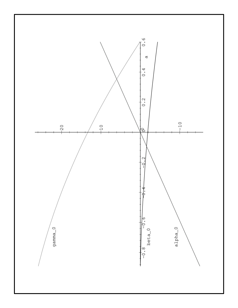
Figure 1: Approximate spectral curve coefficients

In Figure 1, we plot the approximate spectral curve coefficients, $\alpha_{0}$,$\beta_{0}$,$\gamma_{0}$ for $a\in[a_{-},a_{+}]$.

Having discussed the approximate spectral curves it is now time to use the approximate Nahm data for its intended purpose. We take it as input for the numerical ADHMN construction developed in an earlier paper [6]. Figure 2 shows the output, in the form of a surface of constant energy density, for each value of the input parameter $a$. The surfaces shown correspond to the values $a=0.4,0.2,0.1,0.0,-0.1,-0.2,-0.4.$ The low energy 3-monopole scattering process is as follows. Initially, Fig 2.1, there are three unit charge monopoles on the vertices of a contracting equilateral triangle in the $x_{1}x_{2}$-plane. As they merge each monopole raises an arm, so that they link in a kind of maypole dance, Fig 2.2. The legs of the monopoles continue towards the centre, Fig 2.3, until they too merge and the tetrahedral 3-monopole is formed, Fig 2.4. Next the top segment of the tetrahedron separates from the bottom, Fig 2.5, and as it moves up the $x_{3}$-axis it leaves behind a torus with three prongs, Fig 2.6. As the single monopole continues its journey up the $x_{3}$-axis it becomes more spherical, and the 2-monopole smooths out into a torus as it moves down the $x_{3}$ axis.

5 Higgs zeros

Numerical evidence suggests [7, 12] that the tetrahedral 3-monopole has five zeros of the Higgs field, despite the fact that it is a charge three monopole. A scattering geodesic through the tetrahedral 3-monopole has been investigated in detail and the associated dynamics, creation and annihilation of the Higgs zeros tracked numerically [7]. Since the cyclic scattering of three monopoles passes through the tetrahedral 3-monopole, we have an opportunity to study further this novel phenomenon of extra Higgs zeros. We compute an analytical approximation to the Higgs field, and find that it is consistent with a conjectured behaviour of the Higgs zeros.

Finding the Nahm data effectively solves the nonlinear part of the monopole construction but in order to calculate the Higgs field the linear part of the ADHMN construction must also be implemented. Given Nahm data $(T_{1},T_{2},T_{3})$ for a $k$-monopole we must solve the ordinary differential equation

$$({{\upright\hbox to0.0pt{1\hss}\kern 2.0pt1}}_{2k}\frac{d}{ds}+{{\upright\hbox to0.0pt{1\hss}\kern 2.0pt1}}_{k}\otimes x_{j}\sigma_{j}+iT_{j}\otimes\sigma_{j}){\bf v}=0$$ (5.1)

for the complex $2k$-vector ${\bf v}(s)$, where ${\upright\hbox to0.0pt{1\hss}\kern 2.0pt1}_{k}$ denotes the $k\times k$ identity matrix, $\sigma_{j}$ are the Pauli matrices and ${\bf x}=(x_{1},x_{2},x_{3})$ is the point in space at which the Higgs field is to be calculated. Introducing the inner product

$$\langle{\bf v}_{1},{\bf v}_{2}\rangle=\int_{0}^{2}{\bf v}_{1}^{\dagger}{\bf v}_{2}\ ds$$ (5.2)

then the solutions of (5.1) which we require are those which are normalizable with respect to (5.2). It can be shown that the space of normalizable solutions to (5.1) has (complex) dimension 2. If $\widehat{\bf v}_{1},\widehat{\bf v}_{2}$ is an orthonormal basis for this space then the Higgs field $\Phi$ is given by

$$\Phi=i\left[\begin{array}[]{cc}\langle(s-1)\widehat{\bf v}_{1},\widehat{\bf v}_{1}\rangle&\langle(s-1)\widehat{\bf v}_{1},\widehat{\bf v}_{2}\rangle\\ \langle(s-1)\widehat{\bf v}_{2},\widehat{\bf v}_{1}\rangle&\langle(s-1)\widehat{\bf v}_{2},\widehat{\bf v}_{2}\rangle\end{array}\right].$$ (5.3)

The strategy adopted is to use the approximate Nahm data of the previous section and compute approximate solutions of (5.1).

To begin we consider the initial value problem of (5.1) at the pole $s=0$, which has the form

$$s\frac{d{\bf v}}{ds}=B_{s}{\bf v}$$ (5.4)

where $B_{s}$ is a regular $6\times 6$ matrix function of $s\in[0,2)$. This is a regular-singular problem and the eigenvalues of $B_{0}$ are $\{1,1,1,1,-2,-2\}$, hence there is a four-parameter family of solutions which are regular for $s\in[0,2)$. Expressing the solution as a series

$${\bf v}(s)=\sum_{j=1}^{\infty}{\bf d}^{(j)}s^{j}$$ (5.5)

the four arbitrary parameters may be taken to be $d_{1},..,d_{4}$ where

$${\bf d}^{(1)}=(d_{1},d_{2},d_{3},d_{4},i\sqrt{2}d_{2},-i\sqrt{2}d_{3})^{t}.$$ (5.6)

Similarly for the intial value problem at $s=2$ there exists a four-parameter family of solutions $\widetilde{\bf v}(s)$ which are regular for $s\in(0,2]$ and which may be expressed as a series in $\widetilde{s}=2-s$

$$\widetilde{\bf v}(s)=\sum_{j=1}^{\infty}{\bf h}^{(j)}\widetilde{s}^{j}.$$ (5.7)

In this case the four arbitrary parameters are contained in

$${\bf h}^{(1)}=(h_{1},h_{2},h_{3},i\sqrt{2}h_{1},h_{4},ih_{3}/\sqrt{2})^{t}.$$ (5.8)

Taking the solution to be ${\bf v}(s)$ for $s\in[0,1]$ and $\widetilde{\bf v}(s)$ for $s\in[1,2]$ results in the matching condition ${\bf v}(1)=\widetilde{\bf v}(1)$ at $s=1$. Since this is a vector equation with six components this gives six constraints involving the eight arbitrary parameters. We thus obtain the required two parameter family of solutions from which to construct an orthonormal basis.

To perform the approximate ADHMN construction we use the approximate Nahm data (with parameter $a$) of the previous section and truncate the series (5.5) and (5.7) at quartic order. Since all functions are now simple series the required integrals are elementary. The above procedure was implemented using MAPLE. Despite the low order approximations used the calculations are very involved, and to simplify matters we restrict to calculating the Higgs field on the $x_{3}$-axis only. That is, we set $x_{1}=x_{2}=0$ and $x_{3}=L$ in the above. In this case a convenient choice of gauge (equivalent to a choice of orthonormal basis) exists in which the Higgs field is diagonal

$$\Phi=i\left[\begin{array}[]{cc}\varphi&0\\ 0&-\varphi\end{array}\right].$$ (5.9)

The output of the MAPLE program then consists of the function $\varphi$, which depends on the coordinate along the $x_{3}$-axis $L$ and the input parameter $a$, which determines which monopole configuration along the geodesic we are studying. Even in this simplified case the result is rather complicated (the expression fills a full page!). We plot, in Figure 3, $\varphi$ as a function of $L$ for four values of $a$. The first (Figure 3.1) is for $a=0$, which is the tetrahedral 3-monopole. It can be clearly seen that there are two distinct zeros of the Higgs field along this line. One is at the origin and the other is at $L\approx 1$, which is associated with one of the vertices of the tetrahedron. This result is in good agreement with the numerical results of [7, 12]. It confirms that the tetrahedron has four zeros, each with a local winding $+1$, on the vertices of a tetrahedron and a fifth zero, which we refer to as an anti-zero since it has local winding $-1$, at the origin.

The remaining plots in Figure 3 are evidence to support the following conjecture on the dynamics of the Higgs zeros. Initially the three monopoles are well-separated, so there can only be three zeros. They are positioned on the vertices of an equilateral triangle in the $x_{1}x_{2}$-plane. At all times the zeros of the Higgs field must be consistent with the $C_{3}$ symmetry, which leads us to the following description.

The three zeros on the vertices of a triangle approach the $x_{3}$-axis, but fall below the origin. During their approach there is a critical point on the $x_{3}$-axis where there is a zero anti-zero creation event, sending an anti-zero down the $x_{3}$-axis and a plus zero up the $x_{3}$-axis (Figure 3.2, $a=0.05$). The anti-zero reaches the origin (this is the tetrahedral 3-monopole, Figure 3.1, $a=0$) and continues down the $x_{3}$-axis (Figure 3.3, $a=-0.05$) until it eventually meets up with the three positive zeros as they hit the $x_{3}$-axis. Then we have lost all anti-zeros and are left with the $+1$ zero of the unit charge monopole moving up the $x_{3}$-axis and the $+2$ zero of the axisymmetric 2-monopole moving down the $x_{3}$-axis. As a last check we verify that for $a$ sufficiently large there are no zeros on the $x_{3}$-axis (Figure 3.4, $a=0.2$).

From Figure 3 we see that the number of zeros on the $x_{3}$-axis has a simple interpretation. The shape of the $\varphi$ curve remains the same, but as $a$ decreases the curve moves up the plane. Thus the number of roots of this curve increases from zero to an instantaneous double root and finally to two simple roots, with the separation between the two roots then monotonically increasing.

We now address the question of the uniqueness of the above interpretation of the motion of the Higgs zeros drawn from the data. It turns out that there is a second possibility which is more complicated than the first and involves a splitting into anti-zeros of each of the three initial Higgs zeros. The results given so far are consistent with both conjectures and an additional check must be made to decide between the two. For the first possibility, which will turn out to be the correct one, we have seen that for configurations just prior to the formation of the tetrahedral 3-monopole there are two zeros on the $x_{3}$-axis which have a local winding number $+1$ and $-1$ respectively. An analysis of the second possibility demands that these zeros have local winding numbers $+1$ and $+2$. To settle the issue a numerical calculation is performed. First we select a suitable configuration, which is taken to be $a=0.02$. Figure 4 shows a plot of the length squared of the Higgs field (solid line) and a component of the Higgs field (dashed line) along the axis $x_{3}=L$. From this the positions of the two zeros can be approximately read off as $L\approx 0.6$ and $L\approx 0.15$. Next we apply the numerical algorithm given in [7] to compute the local winding number $Q_{R}(L)$ of the normalized Higgs field on a two-sphere of radius $R$, with centre $(x_{1},x_{2},x_{3})=(0,0,L)$. As a first check we compute that $Q_{2}(0)=+3$, so that when all zeros are inside the chosen two-sphere the local winding number indeed gives the number of monopoles. Next we examine the zero which is highest on the $x_{3}$-axis and confirm that $Q_{0.1}(0.6)=+1$. Finally, the computation that $Q_{0.1}(0.15)=-1$ shows that the second zero on the $x_{3}$-axis is an anti-zero and thus rules out the second possibility for the motion of the Higgs zeros to which we alluded above.

For geodesics involving monopoles which are linearized on a quotient curve which is elliptic, it has been conjectured [7, 12] that the special ‘splitting points’, where anti-zeros appear/disappear, are associated to singular points where an elliptic curve becomes rational. Presumably when the geodesic involves monopoles which are linearized on a higher genus surface (as here) the ‘splitting points’ will correspond to vanishing cycle points of the surface.

6 Cyclic 4-monopoles

For $C_{4}$ symmetric 4-monopoles there are three types of geodesics, corresponding to the surfaces $\Sigma_{4}^{0},\Sigma_{4}^{1}$ and $\Sigma_{4}^{2}$. The first of these is the essentially planar scattering where the four monopoles instantaneously form an axially symmetric configuration and subsequently scatter through an angle of $45^{\circ}$. We shall not be concerned with this type of scattering. The other two processes are fully three-dimensional and are of more interest. The $\Sigma_{4}^{2}$ geodesic has an increased symmetry from $C_{4}$ to $D_{4}$ and describes a scattering through the cubic 4-monopole [5]. It is possible to investigate this geodesic in exactly the same manner as was done earlier for the $C_{3}$ geodesic through the tetrahedral 3-monopole. However, the $\Sigma_{4}^{1}$ geodesic does not contain any Platonic monopole configurations, and so at first sight it appears that we require a new ingredient to deal with this case; since we do not know the exact Nahm data at any point on the geodesic we can not read-off the residue behaviour. It turns out that it is instructive not to deal with each case separately, but to apply a unified treatment. This is presented in the following.

First of all, we use equation (3.4) to obtain the form of the Nahm data from the algebra $A_{3}^{(1)}$. It is convenient to change notation and write

$$T_{1}=\frac{1}{2}\left[\begin{array}[]{cccc}0&-q_{1}&0&q_{0}\\ q_{1}&0&-q_{2}&0\\ 0&q_{2}&0&-q_{3}\\ -q_{0}&0&q_{3}&0\end{array}\right];\ T_{2}=-\frac{i}{2}\left[\begin{array}[]{cccc}0&q_{1}&0&q_{0}\\ q_{1}&0&q_{2}&0\\ 0&q_{2}&0&q_{3}\\ q_{0}&0&q_{3}&0\end{array}\right];\$$

$$T_{3}=i\left[\begin{array}[]{cccc}p_{1}&0&0&0\\ 0&p_{2}&0&0\\ 0&0&p_{3}&0\\ 0&0&0&p_{0}\end{array}\right].$$ (6.1)

Nahm’s equation then becomes the set of equations (equivalent to the 4-particle Toda chain)

$$\dot{p}_{j}=\frac{1}{2}(q_{j}^{2}-q_{j-1}^{2}),\hskip 10.0pt\dot{q}_{j}=q_{j}(p_{j}-p_{j+1})$$ (6.2)

where the indices are to be read modulo 4, in accordance with the periodicity of the chain. Since we are considering strongly centred monopoles we also impose the standard Toda chain zero momentum relation

$$\sum_{j=0}^{3}p_{j}=0.$$ (6.3)

We shall generally use this relation to eliminate $p_{0}$ from the equations, but for certain purposes it is useful to preserve the symmetry of the system and not explicitly solve for $p_{0}$.

The spectral curve of the Nahm data (6.1) is

$$\eta^{4}+\alpha\eta^{2}\zeta^{2}+\beta(\zeta^{8}+1)+\gamma\zeta^{4}+\delta\eta\zeta^{3}=0$$ (6.4)

where the real constants are

$$\alpha = \sum_{j=0}^{3}\{q_{j}^{2}+2p_{j}(2p_{j+1}+p_{j+2})\}$$ (6.5)

$$\beta = -\prod_{j=0}^{3}q_{j}$$ (6.6)

$$\gamma = 16\prod_{j=0}^{3}p_{j}+\frac{1}{2}\sum_{j=0}^{3}\{q_{j}^{2}(q_{j+2}^{2}+8p_{j-1}p_{j+2})\}$$ (6.7)

$$\delta = \sum_{j=0}^{3}\{q_{j}^{2}(p_{j-1}+p_{j-2})+8p_{j}p_{j+1}p_{j-1}\}.$$ (6.8)

We now examine the residue behaviour at $s=0$. Putting

$$q_{j}\sim r_{j}/s,\hskip 10.0ptp_{j}\sim R_{j}/s\hskip 28.45274pt\mbox{as}\ s\rightarrow 0$$ (6.9)

into equation (6.2) gives

$$2R_{j}+r_{j}^{2}-r_{j-1}^{2} = 0$$ (6.10)

$$r_{j}(R_{j}-R_{j+1}+1) = 0.$$ (6.11)

Substituting the first of these equations into the second we obtain

$$r_{j}(r_{j+1}^{2}-2r_{j}^{2}+r_{j-1}^{2}+2)=0.$$ (6.12)

Now if all the $r_{j}$ are non-zero then, recognising the bracket as the second order difference approximation to the second derivative, the general solution of the difference equation is

$$r_{j}^{2}=c_{0}+c_{1}j-2j^{2}$$ (6.13)

for constants $c_{0},c_{1}$. However, this solution does not satisfy the periodic boundary conditions $r_{j+4}=r_{j}$, and thus we have proved that at least one of the $r_{j}$’s must be zero.

By symmetry we can choose $r_{0}=0$. All the $R_{j}$’s must be non-zero (in order for the matrix residues to form the irreducible 4-dimensional representation of $su(2)$) which together with equation (6.10) implies that $r_{1}r_{3}\neq 0$. Furthermore, $r_{2}\neq 0$, since if $r_{2}=0$ then the solution is $r_{1}^{2}=r_{2}^{2}=1$ which by equation (6.10) determines $(R_{0},R_{1},R_{2},R_{3})=(1/2,-1/2,1/2,-1/2)$ giving the reducible representation $\underline{2}\oplus\underline{2}$. Now that we have $r_{0}=0$ and $r_{1}r_{2}r_{3}\neq 0$ the equations simplify to the linear system

$$\left[\begin{array}[]{ccc}2&-1&0\\ -1&2&-1\\ 0&-1&2\end{array}\right]\left[\begin{array}[]{c}r_{1}^{2}\\ r_{2}^{2}\\ r_{3}^{2}\end{array}\right]=\left[\begin{array}[]{c}2\\ 2\\ 2\end{array}\right].$$ (6.14)

Note that the matrix occuring in the above is the Cartan matrix of the Lie algebra $A_{3}$. The unique solution is

$$r_{0}=0,\hskip 28.45274ptr_{1}^{2}=3,\hskip 28.45274ptr_{2}^{2}=4,\hskip 28.45274ptr_{3}^{2}=3$$ (6.15)

which gives from equation (6.10) that

$$(R_{0},R_{1},R_{2},R_{3})=(3/2,-3/2,-1/2,1/2)$$ (6.16)

which identifies the matrix residues as forming the required irreducible representation $\underline{4}$.

The upshot is that the only freedom in the choice of residues is which one of the $r_{j}$’s is chosen to be zero. There are some choices of sign available in taking the square roots in (6.15) but these only lead to an inversion of the whole configuration and are of no importance. By a suitable choice of gauge it is always possible to choose $r_{0}=0$ and so at first glance it may appear a puzzle as to how the different types of geodesic are selected. However, there is a similar second pole at $s=2$ at which again one of the associated residues $\widetilde{r}_{j}$ must be zero. Since we are not using a basis in which the symmetry property $T_{i}(2-s)=T_{i}(s)^{t}$ of the Nahm data is manifest, then once the gauge freedom has been used to fix $r_{0}=0$ then we have no freedom left to specify which $\widetilde{r}_{j}$ vanishes. The different geodesics are distinguished by having different $\widetilde{r}_{j}$’s being zero. Another way to view this is that the explicit symmetry transformation relating Nahm data at $s$ to Nahm data at $2-s$ will be different for different geodesics in the same basis. Of course, by general arguments it is true that a basis exists in which the symmetry property is the manifest one given above, but the important point is that this basis is not the same one for different geodesics. This means that there is no point looking for a general “good basis” at the start of the calculation, since this will vary with each solution. It does however mean that all the geodesics can be treated at once and the different cases identified near the end of the calculation by the imposition of the different symmetry properties.

We now construct the approximate twistor data, using the method introduced earlier. A particular solution, which is a single-valued expansion about the $s=0$ pole with residues $r_{j},R_{j}$ as determined above, is constructed for the functions $q_{j},p_{j}$. We omit the details since the method is just as in the $C_{3}$ case considered earlier. Applying Painlev’e analysis gives a linear system with the matrix determinant

$$\Delta=8(r+1)(r+2)(r+3)(r-2)(r-3)(r-4)^{2}$$ (6.17)

giving the Kowalevski exponents. The solution thus contains four arbitrary constants, which is the required number to coincide with the constants $\alpha,\beta,\gamma,\delta$ in the spectral curve.

Again we work with expansions to cubic order in $s$ and take these as the approximate Nahm data for $s\in[0,1]$. To determine a one-parameter family of monopoles we must impose a symmetry relation to construct the Nahm data for the second half of the interval ie. $s\in[1,2]$.

The case $\Sigma_{4}^{2}$

For this geodesic the symmetry property of equations (6.2) which we exploit is the transformation under $s\mapsto 2-s$ of

$$(q_{0},q_{1},q_{2},q_{3}) \mapsto (q_{2},q_{1},q_{0},q_{3})$$ (6.18)

$$(p_{0},p_{1},p_{2},p_{3}) \mapsto (p_{3},p_{2},p_{1},p_{0}).$$ (6.19)

Using this transformed data in the second half of the $s$ interval gives the matching conditions at $s=1$

$$q_{0}(1)=q_{2}(1),\hskip 28.45274ptp_{1}(1)=p_{2}(1),\hskip 28.45274ptp_{1}(1)+p_{2}(1)+2p_{3}(1)=0.$$ (6.20)

Applying these three constraints to the four-parameter family of solutions we arrive at one of the sought after one-parameter families. The constant terms in the spectral curve coefficients are given by

$$\alpha_{0} = 20\sqrt{3}a$$ (6.21)

$$\beta_{0} = \frac{15}{2}+7\sqrt{3}a+4a^{2}$$ (6.22)

$$\gamma_{0} = 105-70\sqrt{3}a+80a^{2}$$ (6.23)

$$\delta_{0} = 0.$$ (6.24)

In fact it is easy to see that the imposed symmetry forces the reductions $q_{1}=q_{3}$ and $p_{3}=-p_{2}$ which in turn gives $\delta=0$ (not just $\delta_{0}=0$). Thus the approximate data has exact $D_{4}$ symmetry. We therefore already know that we are considering either the $\Sigma_{4}^{0}$ or the $\Sigma_{4}^{2}$ geodesic. The confirmation that we have the second of these two possibilities is provided by examination of the approximate spectral curve for $a=0$. This curve is given by

$$\alpha_{0}=0,\hskip 28.45274pt\gamma_{0}=14\beta_{0},\hskip 28.45274pt\beta_{0}=15/2.$$ (6.25)

The first two of these relations are enough to ensure that this curve has cubic symmetry. Thus we have a geodesic containing a cubic configuration and hence are considering the $\Sigma_{4}^{2}$ geodesic. For comparison the exact cubic 4-monopole has a curve given by

$$\alpha=0,\hskip 28.45274pt\gamma=14\beta,\hskip 28.45274pt\beta=3\Gamma(1/4)^{8}/(1024\pi^{2}).$$ (6.26)

Because of the way that $\beta$ enters into the spectral curve it is really the fourth root of $\beta$ which determines the length scale of the cubic monopole. Thus the appropriate comparison is

$$\beta^{1/4}=1.73,\hskip 28.45274pt\beta_{0}^{1/4}=1.65$$ (6.27)

which again demonstrates the reasonable accuracy of such a low order approximation scheme.

Using the same kind of analysis as in the $C_{3}$ case considered earlier, it is possible to determine the range of the parameter $a$ by examining the limiting spectral curves. We apply the numerical ADHMN construction to this approximate Nahm data for the values $a=0.4,0.2,0.1,0.0,-0.1,-0.2,-0.4$. The resulting energy density surfaces are shown in Figure 5. The four monopoles approach on the vertices of a contracting square Fig 5.1, and bend as they merge Fig 5.2, until they form the cube Fig 5.4. The top and bottom portions of the cube then pull apart Fig 5.5, and become increasingly toroidal as the pair of charge 2 monopoles separate along the $x_{3}$-axis Fig 5.7.

The case $\Sigma_{4}^{1}$

For this geodesic the relevant symmetry property of equation (6.2) is the transformation under $s\mapsto 2-s$

$$(q_{0},q_{1},q_{2},q_{3}) \mapsto (q_{1},q_{0},q_{3},q_{2})$$ (6.28)

$$(p_{0},p_{1},p_{2},p_{3}) \mapsto (p_{2},p_{1},p_{0},p_{3})$$ (6.29)

leading to the three matching conditions

$$q_{0}(1)=q_{1}(1),\hskip 28.45274ptq_{2}(1)=q_{3}(1),\hskip 28.45274ptp_{1}(1)+2p_{2}(1)+p_{3}(1)=0.$$ (6.30)

In this case the approximate spectral curve coefficients are a little more complicated

$$\alpha_{0} = 20\sqrt{3}a$$ (6.31)

$$\beta_{0} = -\frac{30\sqrt{3}+a(138+72\sqrt{3})+a^{2}(36+25\sqrt{3})}{9+5\sqrt{3}}$$ (6.32)

$$\gamma_{0} = \frac{-1260-1680\sqrt{3}+a(3360+2100\sqrt{3})+a^{2}(4530+2500\sqrt{3})}{(\sqrt{3}+2)(9+5\sqrt{3})}$$ (6.33)

$$\delta_{0} = \frac{-2400-1200\sqrt{3}+a(2400+1360\sqrt{3})+a^{2}(520+320\sqrt{3})}{(\sqrt{3}+2)(9+5\sqrt{3})}.$$ (6.34)

The salient feature is that $\delta_{0}\neq 0$, so the symmetry is $C_{4}$ and not $D_{4}$, thereby identifying the geodesic as the one associated with the surface $\Sigma_{4}^{1}$.

In figure 6 we show energy density plots for the parameter values

$a=0.6,0.5,0.4,0.3,0.2,0.0$. This scattering appears very similar to the $C_{3}$ scattering discussed earlier. The four monopoles approach on the vertices of a contracting square Fig 6.1, and as they merge they link arms forming a pyramid shaped configuration Fig 6.3. The top of the pyramid breaks off, Fig 6.5, and travels up the $x_{3}$-axis, while the charge three base travels down the $x_{3}$-axis. As they continue to separate, Fig 6.6, the unit charge monopole becomes more spherical and the base deforms closer towards the axisymmetric 3-monopole.

Numerical evidence suggests [12] that the cubic 4-monopole does not possess anti-zeros, in contrast to the tetrahedral 3-monopole. Figures 5 and 6 appear to add some understanding to this result, since it is the $\Sigma_{4}^{1}$ geodesic, rather than the $\Sigma_{4}^{2}$ geodesic, which appears to be the closest 4-monopole analogue of the $\Sigma_{3}^{1}$ geodesic. Hence we might expect the pyramid-like 4-monopole, rather than the cubic 4-monopole to be the one which has anti-zeros.

7 Conclusion

We have proposed an analytical method to obtain approximate Nahm data which, when combined with the previously introduced numerical ADHMN construction, provides an efficient approximation scheme for the construction of monopoles. This has been applied to the study of monopoles with cyclic symmetry and shown to produce good results. The scattering processes reveal exotic dynamics, and indicate that the key to understanding this type of scattering lies with a more detailed knowledge of the zeros of the Higgs field.

Acknowledgements

Many thanks to Nigel Hitchin, Conor Houghton, Nick Manton and Andrew Pickering for useful discussions.

Figure Captions

Fig 1. Approximate spectral curve coefficients

Fig 2. $C_{3}$ symmetric energy density surfaces. The parameter values are                   $a=0.4,0.2,0.1,0.0,-0.1,-0.2,-0.4$

Fig 3. Plot of the Higgs component $\varphi$ on the $x_{3}$-axis, for configurations with $(1)a=0;\ (2)a=0.05;\ (3)a=-0.05;\ (4)a=0.2.$

Fig 4. Plots of the length squared of the Higgs field (solid line) and a Higgs component (dashed line) along the $x_{3}$-axis for $a=0.02$

Fig 5. $D_{4}$ symmetric energy density surfaces. The parameter values are          $a=0.4,0.2,0.1,0.0,-0.1,-0.2,-0.4$

Fig 6. $C_{4}$ symmetric energy density surfaces. The parameter values are          $a=0.6,0.5,0.4,0.3,0.2,0.0$

Note: Figures 2,5 & 6 are attached gif files cyclicfig2.gif etc.

Figure 2: View figure by typing xv cyclicfig2.gif

Figure 3: Plot of the Higgs component $\varphi$ on the $x_{3}$-axis, for configurations with $(1)a=0;\ (2)a=0.05;\ (3)a=-0.05;\ (4)a=0.2.$

Figure 4: Plots of the length squared of the Higgs field (solid line) and a Higgs component (dashed line) along the $x_{3}$-axis for $a=0.02$

References

- [1] M.J. Ablowitz, A. Ramani and H. Segur, J. Math. Phys. 21, 715 (1980).
- [2] M.F. Atiyah and N.J. Hitchin, ‘The geometry and dynamics of magnetic monopoles’, Princeton University Press, 1988.
-
[3]
J.C. Eilbeck, private communication.
V.Z. Enolskii and J.C. Eilbeck, J. Phys. A. 28, 1069 (1995). - [4] N.J. Hitchin, Commun. Math. Phys. 89, 145 (1983).
- [5] N.J. Hitchin, N.S. Manton and M.K. Murray, Nonlinearity, 8, 661 (1995).
- [6] C.J. Houghton and P.M. Sutcliffe, Commun. Math. Phys. 180, 343 (1996).
- [7] C.J. Houghton and P.M. Sutcliffe, Nucl. Phys. B464, 59 (1996).
- [8] A. Kudryavtsev, B. Piette and W.J. Zakrzewski, Phys. Lett. A180, 119 (1993).
- [9] N.S. Manton, Phys. Lett. 110B, 54 (1982).
- [10] W. Nahm, ‘The construction of all self-dual multimonopoles by the ADHM method’, in Monopoles in quantum field theory, eds. N.S. Craigie, P. Goddard and W. Nahm, World Scientific, 1982.
- [11] H. Nakajima, ‘Monopoles and Nahm’s equations’, in Einstein metrics and Yang-Mills connections, Marcel Dekker, New York 1993.
- [12] P.M. Sutcliffe, Phys. Lett. B376, 103 (1996).
- [13] P.M. Sutcliffe, Phys. Lett. B381, 129 (1996).
- [14] H. Yoshida, Cel. Mech. 31, 363 (1983).