Natural renormalization

Abstract

A careful analysis of differential renormalization shows that a distinguished choice of renormalization constants allows for a mathematically more fundamental interpretation of the scheme. With this set of a priori fixed integration constants differential renormalization is most closely related to the theory of generalized functions. The special properties of this scheme are illustrated by application to the toy example of a free massive bosonic theory. Then we apply the scheme to the $\varphi^{4}$-theory. The two-point function is calculated up to five loops. The renormalization group is analyzed, the beta-function and the anomalous dimension are calculated up to fourth and fifth order, respectively.

1 Introduction

With the proof of renormalizability of non-Abelian gauge theories in the early 1970’s the problem of giving a perturbative definition of a renormalizable quantum field theory was solved (eg. [1]). However explicit calculations in the commonly used dimensional regularization are often tedious. This kept the interest in alternative prescriptions alive.

Quite recently differential renormalization [2, 3, 4] has been proposed. For practical calculations this renormalization scheme provides two major advantages. Firstly, it allows to regularize and renormalize in one step. No explicit regulators or counterterms are needed. Secondly, it is possible to keep the spacetime dimension fixed. This is particularly useful for dimension-specific theories like the chiral electroweak sector of the standard model.

We start by analyzing differential renormalization from a purely mathematical point of view. Differential renormalization is usually formulated in four-dimensional coordinate space by writing divergent amplitudes as Laplacians (we restrict ourselves to Euclidean signature, $x^{4}=(x^{2})^{2}$, $\Box=\sum_{i}\partial_{i}^{2}$) of less divergent expressions. For example,

$$\frac{1}{x^{4}{}}=-\frac{1}{4}\Box\frac{1}{x^{2}{}}\ln\left(\frac{x^{2}}{\Lambda_{0}^{2}}\right)\hskip 2.58334pt,\hskip 8.61108pt\hskip 28.45274pt\frac{1}{x^{6}{}}=-\frac{1}{32}\Box\Box\frac{1}{x^{2}{}}\ln\left(\frac{x^{2}}{\Lambda_{1}^{2}}\right)\hskip 8.61108pt\hbox{ for }x\neq 0\hskip 2.58334pt.$$ (1)

$\Lambda_{0}$ and $\Lambda_{1}$ are arbitrary integration constants which are kept for dimensional reasons.

Initially ill-defined integrals are now regularized by the convention that the Laplacian should act on the left and the surface term is ignored. According to this rule the singular Fourier transforms of $x^{-4}$ and $x^{-6}$ can be derived from the well-defined Fourier transform of $x^{-2}\ln(x^{2}{}/\Lambda^{2})$ (calculated below, Eq. (55)),

$$\int\limits_{{\rm diff.ren.\hskip 1.14528pt}}\frac{d^{4}x}{4\pi^{2}{}}\frac{e^{ix\cdot p}}{x^{4}{}} \equiv -\frac{1}{4}\int\frac{d^{4}x}{4\pi^{2}{}}\left(\Box e^{ix\cdot p}\right)\frac{1}{x^{2}{}}\ln\left(\frac{x^{2}}{\Lambda_{0}^{2}}\right)\hskip 4.30554pt=\hskip 4.30554pt-\frac{1}{4}\ln\left(\frac{p^{2}}{\bar{\Lambda}_{0}^{2}}\right)\hskip 2.58334pt,$$ (2)

$$\int\limits_{{\rm diff.ren.\hskip 1.14528pt}}\frac{d^{4}x}{4\pi^{2}{}}\frac{e^{ix\cdot p}}{x^{6}{}} \equiv -\frac{1}{32}\int\frac{d^{4}x}{4\pi^{2}{}}\left(\Box\Box e^{ix\cdot p}\right)\frac{1}{x^{2}{}}\ln\left(\frac{x^{2}}{\Lambda_{1}^{2}}\right)\hskip 4.30554pt=\hskip 4.30554pt\frac{1}{32}p^{2}\ln\left(\frac{p^{2}}{\bar{\Lambda}_{1}^{2}}\right)\hskip 2.58334pt,$$ (3)

where $\bar{\Lambda}_{0(1)}=2/(e^{C}\Lambda_{0(1)})$ and $C$=0.5772156… is the Euler constant.

The central point in this paper is to exhibit the meaning of the above prescriptions for one-dimensional integrals. To this end we perform the convergent angular integrals in (2), (3) which leaves us with a radial integral $\int_{0}^{\infty}dr$ that diverges at $r=0$. We finally split this integral into a convergent part $\int_{1}^{\infty}$ which can be evaluated and a singular part $\int_{0}^{1}$ which is kept. These entirely well-defined manipulations lead to

$$\int\frac{d^{4}x}{4\pi^{2}{}}\frac{e^{ix\cdot p}}{x^{4}{}} = -\frac{1}{2}\left(\ln\left(\frac{e^{C}|p|}{2}\right)-\int_{0}^{1}\frac{dr}{r}-\frac{1}{2}\right)\hskip 2.58334pt,$$ (4)

$$\int\frac{d^{4}x}{4\pi^{2}{}}\frac{e^{ix\cdot p}}{x^{6}{}} = \frac{1}{16}p^{2}\left(\ln\left(\frac{e^{C}|p|}{2}\right)-\int_{0}^{1}\frac{dr}{r}-\frac{5}{4}\right)+\frac{1}{2}\left(\int_{0}^{1}\frac{dr}{r^{3}{}}+\frac{1}{2}\right)\hskip 2.58334pt.$$ (5)

Now we compare this result with Eqs. (2) and (3) derived by differential renormalization. First, notice that the second term on the right hand side of Eq. (5) has no $p^{2}$-dependence at all. To make the right hand side proportional to $p^{2}$ we define

$$\int_{0}^{1}\frac{dr}{r^{3}{}}\equiv-\frac{1}{2}\hskip 2.58334pt.$$ (6)

This leads us finally to the equations

$$\int_{0}^{1}\frac{dr}{r}=-\frac{1}{2}-\ln\Lambda_{0}=-\frac{5}{4}-\ln\Lambda_{1}\hskip 2.58334pt.$$ (7)

Eqs. (6) and (7) can be seen as one-dimensional definitions of differential renormalization. However Eq. (7) naturally relates the renormalization constants via

$$\ln\left(\frac{\Lambda_{1}}{\Lambda_{0}}\right)=-\frac{3}{4}\hskip 2.58334pt.$$ (8)

For a ratio $\Lambda_{1}/\Lambda_{0}$ different from exp(-$\frac{3}{4}$) the one-dimensional interpretation of differential renormalization is not possible.

We will see in the next section that all ratios of renormalization constants are fixed by consistency conditions. Differential renormalization with these a priori fixed ratios will be called ’natural renormalization’.

It was shown [4] that differential renormalization provides a self-consistent definition of renormalizable field theories, without referring to the ratio $\Lambda_{1}/\Lambda_{0}$ as given in Eq. (8). Moreover in some cases it is convenient to adjust the ratios of renormalization constants according to physical requirements [5]. In particular for gauge theories it is useful to fix some ratios by Ward identities [2, 6, 7]. However, depending on the gauge, some of these ratios may differ from the prescriptions we give. The treatment of gauge theories in natural renormalization is still under investigation, first attempts have been successful [8].

The main advantage of allowing for the above one-dimensional reduction and demanding Eqs. (6), (7), (8) is that differential renormalization can be understood on a much more general footing. We will see in Sec. 2.3 that Eqs. (6) and (7) are almost standard in the theory of generalized functions. Thus it becomes possible to replace the recipes of differential renormalization by mathematically more fundamental definitions.

In contrast to differential renormalization, natural renormalization is neither connected to coordinate nor to momentum space. One has the freedom to choose the most convenient representation for the respective problem.

The first example where natural renormalization becomes advantageous is the toy theory of free massive bosons discussed in Sec. 3.1. The mass is treated as two-point interaction which leads by power-counting to a non-renormalizable theory in coordinate space. With standard differential renormalization it becomes necessary to adjust infinitely many constants. It will turn out that these constants coincide with the a priori fixed ratios of our approach. This makes it possible to recover the right result immediately within natural renormalization. This does not happen accidentally as can be shown in a general theorem.

The main application of this paper will be the $\varphi^{4}$-theory in Sec. 3.4. We focus our attention to the calculation of the two-point Green’s function. It will turn out that the $\varphi^{4}$-theory performs almost like made for our renormalization scheme: Most Feynman diagrams of a given order precisely match into a formula which allows to calculate their sum without evaluating single graphs. This enables us to calculate the two-point function up to five loops.

Finally the renormalization group is discussed. The $\beta$-function and the anomalous dimension $\gamma$ are determined up to fourth and fifth order in the coupling, respectively.

2 Definition of the renormalization scheme

2.1 Comparison with differential renormalization

We start with a generalization of the ideas presented in the introduction. Repeated application of the equation

$$\Box f\left(x^{2}\right)=\frac{4}{x^{2}{}}\frac{\partial}{\partial x^{2}{}}x^{4}{}\frac{\partial}{\partial x^{2}{}}f\left(x^{2}\right)$$ (9)

leads to

$$\Box^{n+1}{}\frac{1}{x^{2}{}}\ln\left(\frac{x^{2}}{\Lambda^{2}}\right)=-4^{n+1}n!\left(n+1\right)!\frac{1}{x^{2n+4}{}}\hskip 8.61108pt\hbox{ for }x\neq 0\hskip 2.58334pt,\hskip 8.61108ptn=0,1,{\ldots}\hskip 2.58334pt.$$ (10)

Note that these equations hold strictly only for $x\neq 0$ and may be modified by $\delta(x)$-terms (cf. Eq. (20)). In a renormalizable field theory one needs only a finite number of these equations ($n=0,1$ for the $\varphi^{4}$-theory), however it will turn out to be useful to look at the general case.

The function $x^{-2n-4}$ has no well defined Fourier transform whereas $x^{-2}\ln(x^{2}{}/\Lambda^{2})$ has (cf. Eq. (55)). The differentially renormalized Fourier transform of the right hand side of Eq. (10) is now determined by the left hand side with the Laplacian translated as $-p^{2}$ [2],

$$\int\limits_{{\rm diff.ren.\hskip 1.14528pt}}\frac{d^{4}x}{4\pi^{2}{}}\frac{e^{ix\cdot p}}{x^{2n+4}{}}\equiv\frac{p^{2n}}{\left(-4\right)^{n+1}n!\left(n+1\right)!}\ln\left(\frac{p^{2}}{\bar{\Lambda}_{n}^{2}}\right)\hskip 2.58334pt.$$ (11)

We have introduced different renormalization scales $\bar{\Lambda}_{n}$ for each $n$ to stress that they are integration constants which a priori are independent from each other and may differ by arbitrary positive factors. The $\Lambda_{n}$ are interpreted as renormalization scales.

Our analysis starts with the introduction of polar coordinates.

$$\int\frac{d^{4}x}{4\pi^{2}{}}\frac{e^{ix\cdot p}}{x^{2n+4}{}}=\frac{1}{\pi}\int_{0}^{\pi}d\vartheta\sin^{2}\vartheta\int_{0}^{\infty}drr^{-2n-1}e^{ir|p|\cos\vartheta}\hskip 2.58334pt,$$ (12)

where we have chosen the $z$-axis to be parallel to $p$. We evaluate the convergent $\vartheta$-integral and split the $r$-integral into a convergent part $\int_{1}^{\infty}$ which is evaluated and a part $\int_{0}^{1}$ that diverges at zero and has to remain unchanged.

The calculations are in principle straightforward but tedious [8]. The result is ($\sum_{0}^{-1}\equiv\sum_{1}^{0}\equiv 0$)

$$\int\frac{d^{4}x}{4\pi^{2}{}}\frac{e^{ix\cdot p}}{x^{2n+4}{}} = \sum_{k=0}^{n-1}\frac{p^{2k}}{2\left(-4\right)^{k}k!\left(k+1\right)!}\left(\int_{0}^{1}\frac{dr}{r^{2n-2k+1}{}}+\frac{1}{2n-2k}\right)$$

$$+\frac{2p^{2n}}{\left(-4\right)^{n+1}n!\left(n+1\right)!}\left(-\int_{0}^{1}\frac{dr}{r}+\ln\left(\frac{e^{C}|p|}{2}\right)-\frac{1}{2\left(n+1\right)}-\sum_{k=1}^{n}{}\frac{1}{k}\right)\hskip 2.58334pt.$$

From a mathematical point of view we want $p$-independent integrals to give $p$-independent results. So we are forced to make the following definitions in order to regain the result obtained by differential renormalization (11),

$$\int_{0}^{1}\frac{dr}{r^{2n-2k+1}{}} = -\frac{1}{2n-2k}\hskip 28.45274pt\hbox{\hskip 1.63612ptand\hskip 1.63612pt}$$ (14)

$$\int_{0}^{1}\frac{dr}{r} = -\ln\Lambda_{n}-\frac{1}{2n+2}-\sum_{k=1}^{n}{}\frac{1}{k}\hskip 2.58334pt.$$ (15)

Eq. (14) is the analytic continuation of the formula

$$\int_{0}^{1}drr^{n}{}=\frac{1}{n+1}$$ (16)

to $n<-1$. Eq. (15) shows that within our approach we can not equate the renormalization scales $\Lambda_{n}$ among each other. We find instead

$$\ln\Lambda_{n}=\ln\Lambda-\frac{1}{2n+2}-\sum_{k=1}^{n}{}\frac{1}{k}$$ (17)

for some scale $\Lambda$. The difference $\ln\Lambda_{i}-\ln\Lambda_{j}$ for any $i\neq j$ is a well-defined non-zero rational number. If one violates Eq. (17) one changes the definition of convergent integrals or generates $p$-dependences from $p$-independent divergent integrals. In the differentially renormalized $\varphi^{4}$-theory $\Lambda_{0}$ and $\Lambda_{1}$ are usually equated which however does not destroy the self-consistency of the theory since it is incorporated in the freedom of choosing the renormalization scheme.

An overall factor in the renormalization constants is irrelevant, so we choose a renormalization scale $\Lambda$ according to

$$\int_{0}^{1}\frac{dr}{r}=-\ln\Lambda\hskip 2.58334pt.$$ (18)

Notice that the left hand side of this equation has no explicit $\Lambda$ dependence. One assumes $r^{-1}$ to have the implicit local $\Lambda$-term $-\ln\Lambda\cdot\delta(r)$ in a similar way as the differentially renormalized version of $x^{-4}$ acquires the local renormalization dependence $-\frac{1}{4}\ln\Lambda_{0}^{2}\cdot 4\pi^{2}\delta^{(4)}(x)$ (cf. Eq. (2)).

2.2 First results

’Natural renormalization’ corresponds to differential renormalization with the $\Lambda_{n}$ defined via Eq. (17). It gives a generalization of the usual definition of integrals.

The renormalization scale $\Lambda$ is kept for ’dimensional reasons’. If we integrate over dimensionful parameters then $\Lambda$ combines with other ln-terms to provide a scalar argument of the logarithms. $\Lambda$ is not a cutoff (notice that the integrals over higher order poles (14) are $\Lambda$-independent), it is neither large nor small (cf. Sec. 3.1).

We summarize the above discussion by giving our definition for the singular Fourier transform ($\bar{\Lambda}=2/e^{C}\Lambda$)

$$\int\frac{d^{4}x}{4\pi^{2}{}}\frac{e^{ip\cdot x}}{x^{2n+4}{}}=\frac{p^{2n}}{\left(-4\right)^{n+1}n!\left(n+1\right)!}\left(\ln\left(\frac{p^{2}}{\bar{\Lambda}^{2}}\right)-\frac{1}{n+1}-2\sum_{k=1}^{n}{}\frac{1}{k}\right)\hskip 2.58334pt.$$ (19)

Moreover we can derive this equation in the spirit of differential renormalization by Fourier transforming and translating the Laplacian $\Box$ as $-p^{2}$. But then we have to add $\delta(x)$-terms in Eqs. (1) and (10) which are now uniquely fixed as

$$\Box^{n+1}{}\frac{1}{x^{2}{}}\ln\left(\frac{x^{2}}{\Lambda^{2}}\right)=-4^{n+1}n!\left(n+1\right)!\frac{1}{x^{2n+4}{}}+\left(2\sum_{k=1}^{n}{}\frac{1}{k}+\frac{1}{n+1}\right)\Box^{n}\delta\left(x\right)\hskip 2.58334pt.$$ (20)

The fundamental divergent integrals (16) and (18) are easily generalized to

$$\int_{0}^{1}drr^{n}\ln^{m}\left(r\right) = \frac{\left(-1\right)^{m}m!}{\left(n+1\right)^{m+1}{}}\hskip 2.58334pt,\hskip 8.61108ptn\neq-1\hskip 2.58334pt,\hskip 8.61108ptm\in{N}_{0}\hskip 2.58334pt,$$ (21)

$$\int_{0}^{1}dr\frac{\ln^{m}\left(r\right)}{r} = -\frac{\ln^{m+1}\left(\Lambda\right)}{m+1}\hskip 2.58334pt,\hskip 8.61108ptm\in{N}_{0}\hskip 2.58334pt.$$ (22)

So far we have only discussed singularities located at zero. By translation we can shift the poles to any point of ${R}$. At infinity however one could introduce a new renormalization scale $\Lambda_{\infty}$ according to

$$\int_{1}^{\infty}\frac{dr}{r}=\ln\Lambda_{\infty}\hskip 2.58334pt.$$ (23)

$\Lambda$ should be proportional to $\Lambda_{\infty}$ for dimensional reasons and it is very convenient to set

$$\Lambda=\Lambda_{\infty}\hskip 2.58334pt.$$ (24)

This allows us to generalize Eq. (23) to

$$\int_{1}^{\infty}drr^{n}\ln^{m}\left(r\right) = -\frac{\left(-1\right)^{m}m!}{\left(n+1\right)^{m+1}{}}\hskip 2.58334pt,\hskip 8.61108ptn\neq-1\hskip 2.58334pt,\hskip 8.61108ptm\in{N}_{0}\hskip 2.58334pt,$$ (25)

$$\int_{1}^{\infty}dr\frac{\ln^{m}\left(r\right)}{r} = \frac{\ln^{m+1}\left(\Lambda\right)}{m+1}\hskip 2.58334pt,\hskip 8.61108ptm\in{N}_{0}\hskip 2.58334pt,$$ (26)

and together with Eqs. (21) and (22) we get

$$\int_{0}^{\infty}drr^{n}\ln^{m}\left(r\right)=0\hskip 2.58334pt.$$ (27)

All the integrals defined so far can be summarized by the convention

$$0^{n}\equiv\infty^{n}\equiv 0\hskip 4.30554pt\forall n\neq 0\hskip 2.58334pt,\hskip 8.61108pt\ln 0\equiv\ln\infty\equiv\ln\Lambda\hskip 2.58334pt.$$ (28)

Note that these equations are symmetric under the interchange of zero and infinity which comes from the close connection to analytic continuation.

We close this section with some remarks on changing variables. Integrals that converge at infinity may be shifted by definition. However a naive rescaling $r\mapsto ar$ in Eq. (18) leads to

$$\int_{0}^{1/a}\frac{dar}{ar}=\int_{0}^{1}\frac{dr}{r}+\int_{1}^{1/a}\frac{dr}{r}=-\ln\left(a\Lambda\right)\neq-\ln\Lambda\hskip 2.58334pt.$$ (29)

To keep Eq. (18) invariant under rescalings one has to treat the lower limit zero like a variable and write $\int_{0}^{1}dr/r=\int_{0/a}^{1/a}dr/r=\ln(1/a)-\ln(0/a)=-\ln\Lambda$. Or, equivalently, one rescales the renormalization scale $\Lambda$ according to $\Lambda\mapsto\Lambda/a$. If, like in Eq. (16), the integral does not depend on $\Lambda$, rescalings do not affect the result. For more complicated variable substitutions it is always appropriate to return to the original variables before one approaches the limits (cf. the bipyramide graph in Sec. 3.4.4).

2.3 Relation to the theory of generalized functions

We recognized already in the last section that Eq. (14) can be understood in the context of analytic continuation. In order to include Eq. (18) into this concept one has to ’care for dimensions’ and multiply the integrand by the dimensionless factor $(r/\Lambda)^{\alpha}$, $\alpha\mapsto 0$,

$$\int_{0}^{1}drr^{n}\left(\frac{r}{\Lambda}\right)^{\alpha}=\frac{\Lambda^{-\alpha}}{n+\alpha+1}\hskip 4.30554pt\hskip 2.58334pt,$$

which gives $(n+1)^{-1}$ for $\alpha=0$, $n\neq-1$ and $\alpha^{-1}-\ln\Lambda$ for $n=-1$. If, according to Eq. (28), we replace $\alpha^{-1}$ by zero we are back at (18). Note that analytic continuation is only correct if one uses the factor $(r/\Lambda)^{\alpha}$ and if there exists an $\alpha$-region in ${C}$ where the integral converges. This prescription differs from dimensional regularization by the absence of the surface area $\Omega_{\alpha+1}$. In general the $\alpha$-dependence of $\Omega_{\alpha+1}$ cannot be compensated by a redefinition of the renormalization scale.

There are other contexts in which we can understand the renormalization scheme. Such are contour integrals in the complex plane or lattice theory which generalizes the Riemann sum prescription and eventually provides a purely numerical definition of divergent integrals [8]. Here we present the relation to the theory of generalized functions.

Assume we are interested in an integral which contains the generalized function $f$ that is given as derivative of another generalized function $F^{\prime}=f$. With a test function $\varphi$ we obtain (e.g. [9])

$$\int_{-\infty}^{+\infty}dxf\left(x\right)\varphi\left(x\right)\equiv\left(f,\varphi\right)\equiv\left(F^{\prime},\varphi\right)\equiv-\left(F,\varphi^{\prime}\right)\equiv-\int_{-\infty}^{+\infty}dxF\left(x\right)\varphi^{\prime}\left(x\right)\hskip 2.58334pt.$$ (30)

If $\varphi$ is sufficiently constant at the poles of $F$ the right hand side converges and can be used to define the integral on the left hand side.

Let us e.g. take $f(x)=x^{\lambda}\Theta(x)$; $\Theta(x)=1$ for $x>0$ and $\Theta(x)=0$ for $x<0$. We choose $\varphi=\Theta(1-|x|)$ where the edges at $x=\pm 1$ may be smoothed to be $C^{\infty}$. In the limit where this becomes irrelevant we have for $\lambda\neq-1$

$$\left(f,\varphi\right)=\int_{0}^{1}dxx^{\lambda}\equiv-\int_{0}^{\infty}dx\frac{x^{\lambda+1}}{\lambda+1}\left(-\delta\left(x-1\right)\right)=\frac{1}{\lambda+1}$$ (31)

which coincides with our renormalization rule (16). For $\lambda=-1$ we may take $F(x)=\ln(x)\Theta(x)$ and get

$$\int_{0}^{1}\frac{dx}{x}=-\int_{0}^{\infty}dx\ln\left(x\right)\left(-\delta\left(x-1\right)\right)=0$$ (32)

which is Eq. (18) for $\Lambda=1$. The same holds for Eqs. (21) and (22).

To see what happened with the renormalization scale $\Lambda$ we have to notice that the above calculation is ambiguous. There exist several functions $F$ which have the same derivative. On the real line they differ by a constant which is irrelevant since the test function $\varphi$ vanishes at $\pm\infty$.

In general however the number of undetermined parameters equals the number of disconnected pieces of the integration domain. A singularity of the integrand $f$ at the origin splits ${R}$ into two disconnected parts ${R}^{-}$ and ${R}^{+}$. Each of the functions $F(x)+C+D\Theta(x)$ is with the same right an integral of $f(x)$ on the real line. However they give different results to the integrals (31) and (32),

$$\int\limits_{0}^{1}\!\!dxx^{\lambda}\equiv-\!\!\!\int\limits_{-\infty}^{\infty}dx\left(C_{\lambda}+\Theta\left(x\right)\!\left(\frac{x^{\lambda+1}}{\lambda+1}+D_{\lambda}\right)\!\right)\left(\delta\left(x+1\right)-\delta\left(x-1\right)\right)=\frac{1}{\lambda+1}+D_{\lambda},$$ (33)

$$\int\limits_{0}^{1}\frac{dx}{x}\equiv-\int\limits_{-\infty}^{\infty}dx\left(C_{-1}+\Theta\left(x\right)\left(\ln x+D_{-1}\right)\right)\left(\delta\left(x+1\right)-\delta\left(x-1\right)\right)=D_{-1}\hskip 2.58334pt,$$ (34)

where all the $C_{\lambda}$ and $D_{\lambda}$ can be chosen separately.

The way out of this ambiguity is to change the topology of the integration domain. We can compactify ${R}$ to $\overline{{R}}$ by adding $\infty$ ($=-\infty$). Since for $\lambda<-1$ the integral over $x^{\lambda}$ is well-defined at infinity we can define $F$ over $\overline{{R}}\backslash\{0\}$ which is again a connected domain with one integration constant. The $D_{\lambda}\Theta(x)$ term is discontinuous at infinity and thus no longer allowed in Eq. (33). The integral $\int_{0}^{1}dxx^{\lambda}$ acquires again the unique value $(\lambda+1)^{-1}$.

For $\lambda\geq-1$ the integral diverges at infinity and the gluing is not possible. However for $\lambda>-1$ the integral is finite at $x=0$ and can be defined on the connected domain ${R}$. Just for the case $\lambda=-1$ the ambiguity remains since the integral is divergent both at zero and infinity. The function $\ln|x|$ can only be defined on ${R}^{-}\cup{R}^{+}$ and one should keep the arbitrary constant $D_{-1}$ in Eq. (34). With the more intuitive relabeling $D_{-1}=-\ln\Lambda$ we are back at Eq. (18).

In practice the introduction of the renormalization scale $\Lambda$ is a matter of convenience. It will turn out to be useful to have this parameter at hand. In principle one could set $\Lambda=1$ using the standard theory of generalized functions and recover $\Lambda$ in physical results by getting the dimensions right in logarithmic terms.

3 Applications

Now we turn to physical applications. In the following we are mainly concerned with four-dimensional integrals which we normalize according to

$$\int dx\equiv\int_{{R}^{4}}\frac{d^{4}x}{\left(2\pi\right)^{2}{}}\hskip 28.45274pt\hbox{\hskip 1.63612ptand\hskip 1.63612pt}\hskip 28.45274pt\delta\left(x\right)=\left(2\pi\right)^{2}\delta^{\left(4\right)}\left(\vec{x}\right)\hskip 2.58334pt.$$ (35)

This eliminates all irrelevant factors of $\pi$ from the theory. We get e.g. $\int dx\delta(x)=1$ and $\int dxe^{ip\cdot x}=\delta(p)$. Analogously $n$-dimensional integrals are normalized by $(2\pi)^{(-n/2)}$. The metric is always Euclidean.

3.1 A toy example: the free massive bosonic theory

As a first test let us calculate the four-dimensional free massive boson propagator in coordinate space. The result is well known,

$$\Delta\left(x\right) = \int dp\frac{e^{-ip\cdot x}}{p^{2}+m^{2}{}}=\frac{m}{|x|}K_{1}\left(m|x|\right)$$ (36)

$$= \frac{1}{x^{2}{}}+\frac{m^{2}}{4}\sum_{k=0}^{\infty}\frac{\left(m^{2}x^{2}{}/4\right)^{k}}{k!\left(k+1\right)!}\left(\ln\left(\frac{m^{2}x^{2}}{4}\right)-\Psi\left(k+2\right)-\Psi\left(k+1\right)\right)\hskip 2.58334pt.$$

The propagator $\Delta$ is perfectly well-defined. However it is not analytic at $m=0$ since the series contains logarithmic terms in $m$.

Now let us treat the mass $(-m^{2})$ as a two-point interaction and study perturbation theory around $m=0$.

$$\bullet{-----\mathchoice{\hskip-17.77773pt}{\hskip-17.77773pt}{\hskip-12.77773pt}{\hskip-9.44437pt}\raisebox{0.5pt}{$-----$}\mathchoice{\hskip 2.77773pt}{\hskip 2.77773pt}{\hskip 1.6111pt}{\hskip 0.83331pt}\raisebox{-0.5pt}{$-----$}}\bullet=\bullet-----\bullet+\bullet-----\bullet-----\bullet\mathchoice{\hskip-32.73962pt}{\hskip-32.73962pt}{\hskip-23.91768pt}{\hskip-18.03638pt}\raisebox{-5.59721pt}{$\scriptstyle-m^{2}$}\hskip 29.2777pt+\bullet-----\bullet-----\bullet-----\bullet\mathchoice{\hskip-57.06259pt}{\hskip-57.06259pt}{\hskip-41.61038pt}{\hskip-31.30893pt}\raisebox{-5.59721pt}{$\scriptstyle-m^{2}\hskip 12.05554pt-m^{2}$}\hskip 29.2777pt+{\ldots}$$ (37)

The free propagator in four dimensions is

$$\int dp\frac{1}{p^{2}{}}e^{-ip\cdot x}=\frac{1}{x^{2}{}}\hskip 2.58334pt,$$ (38)

and therefore

$$\Delta\left(x\right)=\frac{1}{x^{2}{}}-m^{2}\int dx_{1}\frac{1}{\left(x\!-\!x_{1}\right)^{2}{}}\frac{1}{x_{1}^{2}{}}+\left(-m^{2}\right)^{2}\int\int dx_{1}dx_{2}\frac{1}{\left(x\!-\!x_{1}\right)^{2}{}}\frac{1}{\left(x_{1}\!-\!x_{2}\right)^{2}{}}\frac{1}{x_{2}^{2}{}}+{\ldots}\hskip 2.58334pt.$$ (39)

Since the ’coupling’ has mass-dimension the terms become more divergent with every order and the expansion is non-renormalizable. However we can treat the integrals according to our rules and obtain an unambiguous result which contains by construction only one renormalization scale $\Lambda$.

In order to evaluate the integrals we can use $\Box(x-x_{1})^{-2}=-\delta(x-x_{1})$ and Eq. (2) to derive a recursive formula. Here it is even simpler to remember that the $n$-th term is the Fourier transform of $p^{-2n}$. Eq. (19) gives

$$\Delta_{{\rm nat.ren.\hskip 1.14528pt}}\left(x\right) = \frac{1}{x^{2}{}}+\sum_{k=0}^{\infty}\left(-m^{2}\right)^{k+1}\int dp\frac{1}{p^{2k+4}{}}e^{ip\cdot x}$$ (40)

$$= \frac{1}{x^{2}{}}+\frac{m^{2}}{4}\sum_{k=0}^{\infty}\frac{\left(m^{2}x^{2}{}/4\right)^{k}}{k!\left(k+1\right)!}\left(\ln\left(\frac{\Lambda^{2}x^{2}}{4}\right)-\Psi\left(k+2\right)-\Psi\left(k+1\right)\right)\!.$$

One could study the renormalization group by looking at rescalings of $\Lambda$. In fact comparison with Eq. (36) shows that the situation is even simpler. We just have to equate $\Lambda=m$ to obtain precisely the correct result. This does not happen accidentally as we will see in the next section.

The differentially renormalized result can be obtained by using Eq. (11) instead of Eq. (19),

$$\Delta_{{\rm diff.ren.\hskip 1.14528pt}}\left(x\right) = \frac{1}{x^{2}{}}+\frac{m^{2}}{4}\sum_{k=0}^{\infty}\frac{\left(m^{2}x^{2}{}/4\right)^{k}}{k!\left(k+1\right)!}\left(\ln\left(\frac{\Lambda_{k}^{2}x^{2}}{4}\right)-2C\right)\hskip 2.58334pt.$$ (41)

It is necessary to adjust the infinitely many parameters $\Lambda_{k}$ precisely according to the a priori settings (17) of our scheme.

Dimensional regularization leads to a series in $4-n$ with a simple pole,

$$\Delta_{{\rm dim.reg.\hskip 1.14528pt}}\left(x\right) = \frac{1}{x^{2}{}}+\frac{m^{2}}{4}\sum_{k=0}^{\infty}\frac{\left(m^{2}x^{2}{}/4\right)^{k}}{k!\left(k+1\right)!}\left(\frac{2}{4-n}+\ln\left(\frac{\Lambda^{2}x^{2}}{2}\right)-\Psi\left(k+1\right)\right)\hskip 2.58334pt.$$ (42)

Since the series is non-renormalizable, it is not possible to renormalize by introducing a finite number of counter terms. If one nevertheless tries to follow a minimum subtraction prescription, one misses a term $-\Psi(k+2)$ to obtain the correct result. In the next section we will present a general method that allows us to calculate this term.

3.2 A theorem on singular expansions

Let us summarize what we did in the last section. We started from a well-defined integral $\int dp\exp(-ip\cdot x)/(p^{2}+m^{2})$ which we tried to expand into a series at $m=0$. To this end we expanded the integrand into a power series $\int dp\exp(-ip\cdot x)\sum_{k=0}^{\infty}(-m^{2})^{k}p^{-2k-2}$. The interchange of the sum and the integral led us to the perturbation series in coordinate space $\sum_{k=0}^{\infty}(-m^{2})^{k}\int dp\exp(-ip\cdot x)p^{-2k-2}$. This interchange is obviously illegal. Firstly, the integrals diverge at $p=0$. Secondly, we obtain a power series in $m$ and we know that the correct result has no such representation but contains logarithmic terms in $m$ (Eq. (36)). Although the integrand is analytic at $m=0$ the integral is not. So necessarily the expansion is wrong and the diverging integrals reflect this fact. We want to study the issue how to reconstruct the true result from such an incorrect, singular expansion.

Let us slightly generalize the situation and look for the expansion of an integral $I(a)=\int dxf(x,a)$ into a series at $a=0$. The integrand has a Taylor (or Laurant) series $f(x,a)=\sum_{k}a^{k}f^{(k)}(x,0)/k!$, but in general we can not expect that the series of $I(a)$ is given by the integrals over the coefficients $f^{(k)}(x,0)$ since the integrals may diverge. We define

$$\Delta I\left(a\right)=\int dxf\left(x,a\right)-\sum_{k}\frac{a^{k}}{k!}\int dxf^{\left(k\right)}\left(x,0\right)\hskip 2.58334pt,$$ (43)

and conclude that $\Delta I(a)$ will only be zero if $I(a)$ is analytic at $a=0$. So $\Delta I(a)$ gives the part of the expansion of $I(a)$ that can not be reached by standard perturbation theory.

We call $\Delta I$ the non-perturbative part of the expansion. A priori we know almost nothing about it. However in many cases where $I(a)$ is not analytic at $a=0$ one can calculate $\Delta I(a)$ by the following theorem.

Theorem. Assume the integrals $\int dxf^{(k)}(x,0)$ are regular at $x\neq 0$. If there exists a neighborhood of $x=0$, $a=0$ where $f$ can be written as $f=\sum_{\ell}f_{\ell}$ with $f_{\ell}(x,a)$ integrable at $x=0$ and the $f_{\ell}^{(k)}(x,0)$ having the following properties

$$f_{\ell}^{\left(k\right)}\left(|x|,0\right)\propto|x|^{n\left(k,\ell\right)}\ln^{m\left(k,\ell\right)}\left(|x|\right)\hskip 8.61108pt\hbox{\hskip 1.63612ptwith\hskip 1.63612pt}$$ (46)

$$\hbox{\hskip 1.63612ptgiven }\ell:\hskip 8.61108pt\lim_{k\rightarrow\infty}n\left(k,\ell\right)/k<0\hbox{ or }f_{\ell}^{\left(k\right)}\left(x,0\right)\equiv 0\hbox{ for almost all{} }k\hskip 8.61108pt\hbox{\hskip 1.63612ptand\hskip 1.63612pt}$$

$$\hbox{\hskip 1.63612ptgiven }k:\hskip 8.61108ptn\left(k,\ell\right)\geq 0\hbox{ for almost all }\ell\hskip 2.58334pt,$$

then

$$\Delta I\left(a\right)=\sum_{\ell}\int dxf_{\ell}\left(x,a\right)\hskip 2.58334pt.$$ (47)

Note that all the integrals may diverge and have to be defined according to the rules given above. The range of integration can be ${R}^{n}$ or ${R}^{+}$, subsets can be taken into account by using step-functions.

Proof (sketch). Without restriction we can assume that the support of $f$ is a little ball $B_{\varepsilon}$ around $x=0$ since the integrals over the remaining domain are regular and therefore do not contribute to $\Delta I$. Moreover we can assume $|a|$ to be small, so that we can write $f$ as a sum over $f_{\ell}$. Since the $f_{\ell}$ are integrable at $x=0$ one gets for sufficiently small $\varepsilon$

$$\int_{B_{\varepsilon}}dxf\left(x,a\right) = \sum_{\ell}\int_{B_{\varepsilon}}dxf_{\ell}\left(x,a\right)$$

$$= \sum_{\ell}\int_{{R}^{n}}dxf_{\ell}\left(x,a\right)-\sum_{\ell}\int_{{R}^{n}\backslash B_{\varepsilon}}dx\sum_{k}\frac{a^{k}}{k!}f_{\ell}^{\left(k\right)}\left(x,0\right)\hskip 2.58334pt.$$

In the second integral the singularity at $x=0$ is excluded and (46) assures that the sum can be interchanged with the integral for small enough $a$, yielding

$$\int_{B_{\varepsilon}}dxf\left(x,a\right)=\sum_{\ell}\int_{{R}^{n}}dxf_{\ell}\left(x,a\right)+\sum_{\ell}\sum_{k}\frac{a_{k}}{k!}\left(\int_{B_{\varepsilon}}-\int_{{R}^{n}}\right)dxf_{\ell}^{\left(k\right)}\left(x,0\right)\hskip 2.58334pt.$$

Now we can use the central argument of the proof. The last integral over the entire ${R}^{n}$ vanishes since (Eq. (46)) it is proportional to $\int_{0}^{\infty}dr\,r^{N}\ln^{M}(r)$ and all those integrals are zero in our renormalization scheme (Eq. (27)). We finally use Eq. (46) to interchange the second sum over $\ell$ with the sum over $k$ and the integral. Therefore

$$\Delta I\left(a\right)\equiv\int_{B_{\varepsilon}}dxf\left(x,a\right)-\sum_{k}\frac{a^{k}}{k!}\int_{B_{\varepsilon}}dxf^{\left(k\right)}\left(x,0\right)=\sum_{\ell}\int_{{R}^{n}}dxf_{\ell}\left(x,a\right)\hskip 2.58334pt.$$

$\Box$

Now let us use the theorem to derive $\Delta I(m^{2})$ of the scalar bosonic theory. We get $f(p,m^{2})=e^{-ip\cdot x}/(p^{2}+m^{2})$. Expanding the exponential yields $f(p,m^{2})=\sum_{\ell}(-ip\cdot x)^{\ell}{}/(\ell!(p^{2}+m^{2}))\equiv\sum_{\ell}f_{\ell}(p,m^{2})$. Moreover $f_{\ell}^{(k)}(p,0)=(-ip\cdot x)^{\ell}(-1)^{k}k!p^{-2-2k}{}/\ell!$ and $f_{\ell}^{(k)}(|p|,0)\propto|p|^{\ell-2-2k}$ meets Eqs. (46), (46), (46). We can apply the theorem and obtain

$$\Delta I_{{\rm nat.ren.\hskip 1.14528pt}}\left(m^{2}\right)=\sum_{\ell=0}^{\infty}\int\frac{d^{4}x}{4\pi^{2}{}}\frac{\left(-ip\cdot x\right)^{\ell}}{\ell!\left(p^{2}+m^{2}\right)}=\sum_{\ell=0}^{\infty}\frac{\left(-i|x|\right)^{\ell}}{\ell!}\frac{1}{\pi}\int_{0}^{\pi}d\vartheta\sin^{2}\vartheta\cos^{\ell}\vartheta\int_{0}^{\infty}\frac{dpp^{\ell+3}}{p^{2}+m^{2}{}}.$$ (48)

The $\vartheta$-integral vanishes for odd $\ell$. The divergent $p$-integral can be reduced to fundamental integrals as follows: $\int_{0}^{\infty}dpp^{2\ell+3}{}/(p^{2}+m^{2})=\int_{0}^{\infty}pdp((p^{2}+m^{2})-m^{2})^{\ell+1}{}/(p^{2}+m^{2})$. With Eq. (27) we obtain $(-m^{2})^{\ell+1}\int_{0}^{\infty}pdp/(p^{2}+m^{2})=\frac{1}{2}(-m^{2})^{\ell+1}\ln(p^{2}+m^{2})|^{\infty}_{0}=\frac{1}{2}(-m^{2})^{\ell+1}\ln(\Lambda^{2}{}/m^{2})$ (with Eq. (28)). The result is proportional to $\ln(\Lambda/m)$ and vanishes thus for $\Lambda=m$. This confirms the explicit calculation of the last section.

The above theorem holds for any spacetime dimension. Hence it should as well be possible to apply it to the dimensionally regularized result and ’correct’ Eq. (42) by adding the non-perturbative part. We start with the $n$-dimensional analogon of Eq. (48). All integrals are standard and one obtains

$$\Delta I_{{\rm dim.reg.\hskip 1.14528pt}}\left(m^{2}\right) = \sum_{\ell=0}^{\infty}\frac{\left(-i|x|\right)^{\ell}}{\ell!}\frac{\Omega_{n-1}}{\left(2\pi\right)^{n/2}{}}\Lambda^{4-n}{}\int_{0}^{\pi}d\vartheta\sin^{n-2}\vartheta\cos^{\ell}\vartheta\int_{0}^{\infty}\frac{dpp^{\ell+n-1}}{p^{2}+m^{2}{}}$$

$$= \sum_{\ell=0}^{\infty}\frac{m^{2}\left(-x^{2}m^{2}\right)^{\ell}}{2^{\ell+2}\ell!}\left(\frac{m^{2}}{2\Lambda^{2}}\right)^{\left(n-4\right)/2}\Gamma\left(\frac{4-n}{2}-\ell-1\right)$$

$$= \sum_{\ell=0}^{\infty}\frac{m^{2\ell+2}x^{2\ell}}{4^{\ell+1}\ell!\left(\ell+1\right)!}\left(-\frac{2}{4-n}-\Psi\left(\ell+2\right)+\ln\left(\frac{m^{2}}{2\Lambda^{2}}\right)\right)+{\cal O}\left(4-n\right).$$

Together with $\Delta_{{\rm dim.reg.\hskip 1.14528pt}}$ (Eq. (42)) the renormalization scale drops out and one obtains the full propagator.

So in the example of a free massive bosonic theory we do not have to go through the standard renormalization business. One can use the above theorem instead. The simplest way to expand the propagator is using natural renormalization, however dimensional regularization leads eventually to the same result.

In a realistic field theory with dimensionless coupling the situation is slightly different. The path integral is a priori ill-defined and the renormalization scale an intrinsic parameter of the theory (like e.g. in the integral $\int_{0}^{1}\frac{dx}{x}=-\ln\Lambda$). It makes no sense to equate the renormalization parameter $\Lambda$ with the coupling. However it is challenging to try to generalize the theorem to path integrals providing a non-perturbative but analytic definition of a quantum field theory.

Anyway the theorem on its own is useful in many elementary mathematical applications. Integrals like $\int_{0}^{b}dx/(x^{n}+a^{n})$, $\int_{0}^{1}dx\ln^{m}(x/\Lambda)/(x+a)$, $\int_{0}^{\infty}dxe^{-bx}/(x+a)^{n}$, $\int_{0}^{\infty}dxe^{-bx-a/x}$, etc. can be expanded at $a=0$ by virtue of the theorem [8].

3.3 Fourier transforms

Before we start to study $\varphi^{4}$-theory it is useful to discuss Fourier transforms since many Feynman amplitudes are determined by multiplications and convolutions.

To this end we generalize the Fourier transforms discussed in the beginning (Eq. (19)). It is convenient to derive the result by analytic continuation. A straightforward calculation gives ($\bar{\Lambda}=2/(e^{C}\Lambda)$)

$$\int\!\frac{d^{4}x}{\left(2\pi\right)^{2}{}}\frac{e^{ip\cdot x}}{x^{2n+4}{}}\left(\frac{x^{2}}{\Lambda^{2}}\right)^{\!-\alpha} = \frac{p^{2n}}{2^{2n+2}{}}\left(\frac{p^{2}}{\bar{\Lambda}^{2}}\right)^{\!\alpha}{}\frac{e^{-2C\alpha}\Gamma\left(-n-\alpha\right)}{\Gamma\left(n+2+\alpha\right)}\equiv\frac{p^{2n}}{2^{2n+2}{}}\left(\frac{p^{2}}{\bar{\Lambda}^{2}}\right)^{\!\alpha}\sum_{\ell=-1}^{\infty}a_{n,\ell}\alpha^{\ell},\hskip 12.91663pt$$ (50)

$$\hbox{\hskip 1.63612ptwhere\hskip 1.63612pt}\hskip 12.91663pt\sum_{\ell=-1}^{\infty}a_{n,\ell}\alpha^{\ell} = \frac{\Gamma\left(-n-\alpha\right)}{\Gamma\left(1-\alpha\right)}\frac{\Gamma\left(1+\alpha\right)}{\Gamma\left(n+2+\alpha\right)}\exp\left(\sum_{k=1}^{\infty}\frac{2\zeta\left(2k+1\right)}{2k+1}\alpha^{2k+1}\right)\hskip 2.58334pt.$$ (51)

Now it is easy to determine all Fourier transforms of the form $x^{-2n-4}\ln^{m}(x^{2}{}/\Lambda^{2})$. To produce the logarithms we divide Eq. (50) by $\alpha^{m}$ and pick up the finite term in the $\alpha$-expansion:

$$\int dx\frac{\ln^{m}\left(x^{2}{}/\Lambda^{2}\right)}{x^{2n+4}{}}e^{ip\cdot x}=\left(-1\right)^{m}m!\frac{p^{2n}}{2^{2n+2}{}}\sum_{\ell=-1}^{\infty}a_{n,\ell}g_{\ell-m}\left(\frac{p^{2}}{\bar{\Lambda}^{2}}\right)\hskip 2.58334pt,$$ (52)

where $g_{\ell}(p^{2}{}/\bar{\Lambda}^{2})$ is the finite term of $(p^{2}{}/\bar{\Lambda}^{2})^{\alpha}\alpha^{\ell}$ at $\alpha=0$. We obtain $g_{\ell}=\ln^{|\ell|}(p^{2}{}/\bar{\Lambda}^{2})/|\ell|!$ for $\ell\leq 0$. For $\ell$ positive $g_{\ell}(p^{2}{}/\bar{\Lambda}^{2})=0$ for all $p\neq 0$. A more detailed calculation [8] shows that $p^{-4}g_{1}(p^{2}{}/\bar{\Lambda}^{2})=\frac{1}{4}\delta(p)$.

Let us take e.g. $n=1$ yielding $\sum_{\ell=-1}^{\infty}a_{1,\ell}\alpha^{\ell}=\frac{1}{2}\alpha^{-1}{}-\frac{5}{4}+\frac{17}{8}\alpha+(-\frac{49}{64}+\frac{1}{3}\zeta(3))\alpha^{2}+{\cal O}(\alpha^{3})$ and therefore (cf. Eq. (19))

$$\int dxe^{ip\cdot x}\frac{1}{x^{6}} = \frac{1}{16}p^{2}\left(\frac{1}{2}\ln\left(\frac{p^{2}}{\bar{\Lambda}^{2}}\right)-\frac{5}{4}\right)\hskip 2.58334pt,$$ (53)

$$\int dxe^{ip\cdot x}\frac{\ln\left(x^{2}{}/\Lambda^{2}\right)}{x^{6}} = \frac{1}{16}p^{2}\left(-\frac{1}{4}\ln^{2}\left(\frac{p^{2}}{\bar{\Lambda}^{2}}\right)+\frac{5}{4}\ln\left(\frac{p^{2}}{\bar{\Lambda}^{2}}\right)-\frac{17}{8}\right)\hskip 2.58334pt.$$ (54)

$n=-1$ gives $\sum_{\ell=-1}^{\infty}a_{-1,\ell}\alpha^{\ell}=1+\frac{2}{3}\zeta(3)\alpha^{3}+{\cal O}(\alpha^{5})$, thus

$$\int dxe^{ip\cdot x}\frac{1}{x^{2}{}}=\frac{1}{p^{2}{}}\hskip 2.58334pt,\hskip 8.61108pt\hskip 28.45274pt\int dxe^{ip\cdot x}\frac{\ln\left(x^{2}{}/\Lambda^{2}\right)}{x^{2}{}}=-\frac{\ln\left(p^{2}{}/\bar{\Lambda}^{2}\right)}{p^{2}{}}\hskip 2.58334pt.$$ (55)

With $n=-2$ we finally obtain the standard formula $\int dxe^{ip\cdot x}=\delta(p)$. Less obvious is $\int dxe^{ip\cdot x}\ln(x^{2}{}/\Lambda^{2})=-4p^{-4}+\delta(p)$.

3.4 The massless $\varphi^{4}$-theory

The first serious test of the renormalization scheme is the discussion of the $\varphi^{4}$-theory. Note that once the Feynman rules and the propagator are fixed the results are unique. There is no freedom to choose a certain subtraction scheme.

We keep our integral normalization of $(2\pi)^{-2}$ which results in a rescaling of the coupling by $(2\pi)^{2}$. So $g$ is related to the usual ’irrationalized’ coupling via

$$\frac{g}{4}=\frac{\lambda}{16\pi^{2}{}}\hskip 2.58334pt.$$ (56)

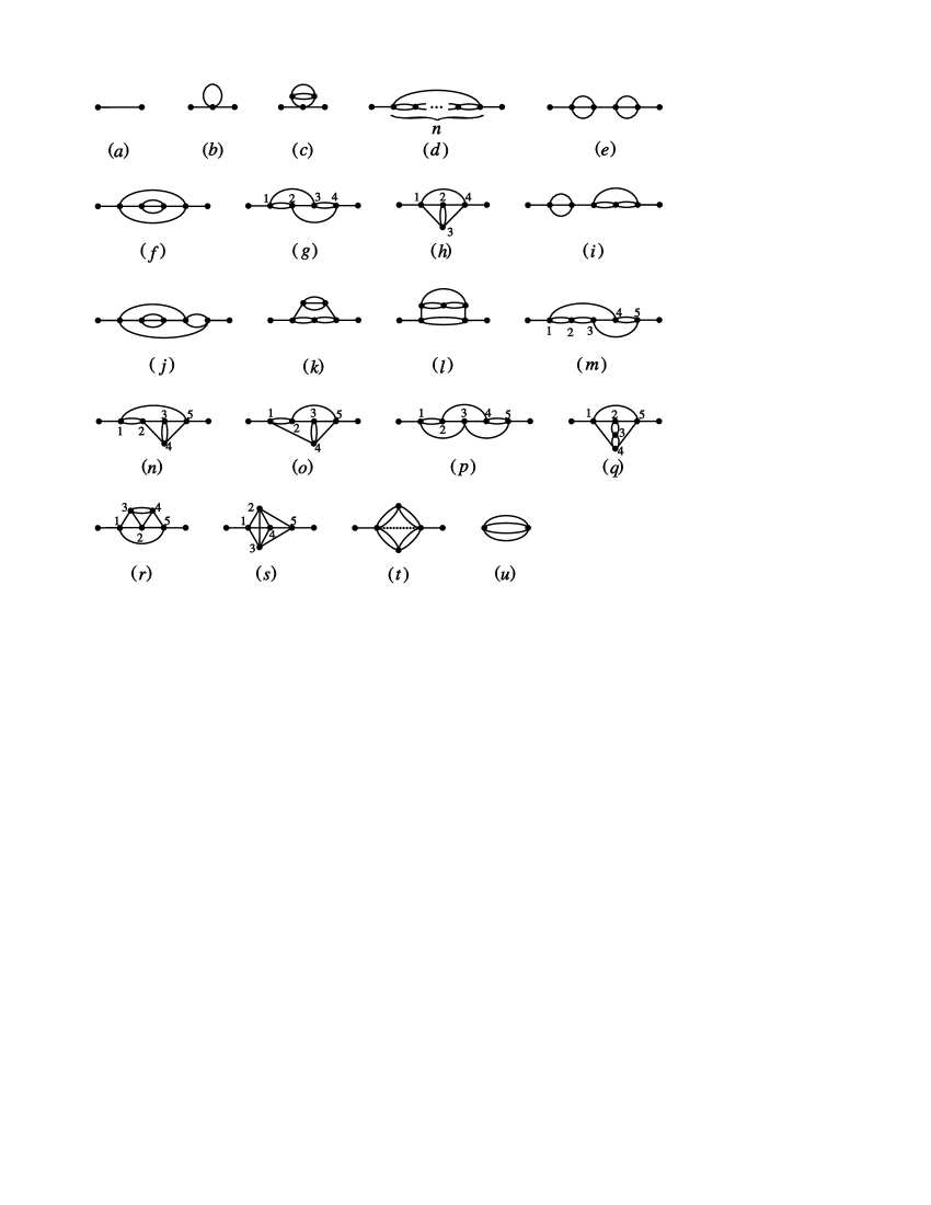
Figure 1: Feynman diagrams of the $\varphi^{4}$-theory.

The Feynman diagrams we are concerned with are depicted in Fig. 1 ($a$), …, ($u$). The corresponding amplitudes are labeled by $G_{a}$, …, $G_{u}$. With natural renormalization we have the freedom to switch between coordinate and momentum space. However, most often it is convenient to start the calculation in coordinate space where, at least at higher loops, the Feynman rules are more transparent. The final result is given in momentum space to make it easier to compare it with other work.

3.4.1 Simple results

The free propagator ($a$) is given by $G_{a}=p^{-2}$.

The loop in the diagram ($b$) gives rise to a term $\int dpp^{-2}$ in momentum space or a term $(x-x)^{-2}{}=0^{-2}$ in coordinate space. Both expressions are set to zero in our scheme: $G_{b}=0$. In this aspect it behaves like dimensional regularization.

More generally, diagrams that contain tadpole insertions give zero and can be dropped. This remains true for any number of internal lines the tadpole may have: $G_{c}=0$. The reason is that in a massless theory a tadpole insertion can only give rise to a number times a momentum conserving $\delta$-function. On the other hand it has dimension $p^{2}$ and the only number with this scaling property is zero. In our renormalization scheme $\bar{\Lambda}^{2}$ occurs only in combination with logarithms.

Moreover, due to translation invariance and Eq. (27), all vacuum bubbles vanish: $G_{u}=0$. So only connected diagrams contribute to the two-point function. Altogether this reduces the number of relevant Feynman diagrams considerably.

Diagram ($d$) for $n=1$ is the sunset diagram. It was already calculated in the last section. The triple line gives $x^{-6}$ which transforms into momentum space as $(\frac{p}{4})^{2}(\frac{1}{2}\ln(p/\bar{\Lambda})^{2}-\frac{5}{4})$. Together with the two external legs and the symmetry factor $\frac{1}{6}$ we obtain

$$G_{d,1}=\left(\frac{g}{4}\right)^{2}{}\frac{1}{p^{2}{}}\left(\frac{1}{12}\ln\left(\frac{p^{2}}{\bar{\Lambda}^{2}}\right)-\frac{5}{24}\right)\hskip 2.58334pt.$$ (57)

3.4.2 Chain graphs

We call diagrams of type ($d$) chain graphs. To any order there exists one chain graph and, if we disregard the vanishing diagrams with tadpoles, the only remaining diagrams up to three loops are chain graphs.

It is possible to calculate chain graph amplitudes for any $n$ by Fourier transformation. In momentum space the series of bubbles gives rise to the $n$-th power of $\frac{1}{4}(-\ln(p/\bar{\Lambda})^{2}+1)$ (cf. Eq. (19)). A final convolution with $p^{-2}$ (use Eq. (9) as suggested in Sec. 3.1) provides the result as an $n$-th order polynomial in $\ln(p/\bar{\Lambda})^{2}$ with purely rational coefficients. Including the symmetry factors and the external legs we obtain for $n\geq 2$ (the case $n=1$ has an extra symmetry which changes the symmetry factor from $2^{-n}$ to $\frac{1}{6}$)

$$G_{d,n}=\left(\frac{g}{4}\right)^{n+1}{}\frac{1}{p^{2}{}}\frac{n!}{2^{n+1}{}}\sum_{k=0}^{n}\left(-1\right)^{k}\frac{\ln^{n-k}\left(p/\bar{\Lambda}\right)^{2}}{\left(n-k\right)!}\sum_{\ell=0}^{k}\frac{2-2^{\ell-k}}{\ell!}\hskip 2.58334pt.$$ (58)

There is a nice way to compile this result by a generating function. If we multiply $G_{d,n}$ with the factor $a_{n}=3^{n-2}$ for $n\geq 2$, $a_{1}=1$, it reproduces the leading logarithms of the full $\varphi^{4}$ two-point function correctly. The result may be seen as some approximation to the propagator. We get

$$\sum_{n=1}^{\infty}\frac{a_{n}G_{d,n}}{n!}=\frac{g}{9p^{2}{}}\left(\frac{\left(p^{2}{}/e\bar{\Lambda}^{2}\right)^{3g/8}}{9\left(1+g/4\right)^{2}-1}-\frac{1}{8}\right)\hskip 2.58334pt.$$ (59)

We easily read off

$$G_{d,2} = \left(\frac{g}{4}\right)^{3}\!\frac{1}{p^{2}{}}\!\left(\frac{1}{8}\ln^{2}\!\left(\frac{p^{2}}{\bar{\Lambda}^{2}}\right)-\frac{5}{8}\ln\!\left(\frac{p^{2}}{\bar{\Lambda}^{2}}\right)+\frac{15}{16}\right)$$ (60)

$$G_{d,3} = \left(\frac{g}{4}\right)^{4}\!\frac{1}{p^{2}{}}\!\left(\frac{1}{16}\ln^{3}\!\left(\frac{p^{2}}{\bar{\Lambda}^{2}}\right)-\frac{15}{32}\ln^{2}\!\left(\frac{p^{2}}{\bar{\Lambda}^{2}}\right)+\frac{45}{32}\ln\!\left(\frac{p^{2}}{\bar{\Lambda}^{2}}\right)-\frac{109}{64}\right)$$ (61)

$$G_{d,4} = \left(\frac{g}{4}\right)^{5}\!\frac{1}{p^{2}{}}\!\left(\frac{1}{32}\ln^{4}\!\left(\frac{p^{2}}{\bar{\Lambda}^{2}}\right)-\frac{5}{16}\ln^{3}\!\left(\frac{p^{2}}{\bar{\Lambda}^{2}}\right)+\frac{45}{32}\ln^{2}\!\left(\frac{p^{2}}{\bar{\Lambda}^{2}}\right)-\frac{109}{32}\ln\!\left(\frac{p^{2}}{\bar{\Lambda}^{2}}\right)+\frac{239}{64}\right)\!.$$ (62)

3.4.3 Four loops

Before we start with the analysis of four and five loops a word of caution is in order. In general it is not sufficient to define the integral over generalized functions for defining a field theory, since also products of generalized functions appear. In principle e.g. one has to consider terms like $x^{2}\delta(x)$ since they might give finite contributions after multiplication with $x^{-2}$.

In the following we do not care about such terms. The main message of the next two subsections is to show that there is a miraculous matching of Feynman amplitudes in the natural renormalization scheme that makes calculations easy. This matching is not affected by the above problems nor are the leading logarithms of the results. This is confirmed by the existence of the renormalization group equation studied in Sec. 3.4.6.

Diagrams ($e$), ($f$), ($g$), and ($h$) remain to be evaluated. $G_{e}$ is basically the square of $G_{d,1}$.

$$G_{e}=\left(\frac{g}{4}\right)^{4}{}\frac{1}{p^{2}{}}\left(\frac{1}{144}\ln^{2}\left(\frac{p}{\bar{\Lambda}}\right)^{2}{}-\frac{5}{144}\ln\left(\frac{p}{\bar{\Lambda}}\right)^{2}{}+\frac{25}{576}\right)\hskip 2.58334pt.$$ (63)

$G_{f}$ can be calculated with Fourier transforms. Adding propagators from the interior loop to the exterior lines we obtain (see Eqs. (53)–(55))

$$\frac{1}{x^{6}{}}\stackrel{{\scriptstyle{\cal F}}}{{\longrightarrow}}\frac{p^{2}}{4^{2}{}}\left(\frac{1}{2}\ln\left(\frac{p}{\bar{\Lambda}}\right)^{2}\!\!-\frac{5}{4}\right)\stackrel{{\scriptstyle p^{-4}}}{{\longrightarrow}}\frac{1}{4^{2}p^{2}{}}\left(\frac{1}{2}\ln\left(\frac{p}{\bar{\Lambda}}\right)^{2}\!\!-\frac{5}{4}\right)\stackrel{{\scriptstyle{\cal F}}}{{\longrightarrow}}\frac{1}{4^{2}x^{2}{}}\left(-\frac{1}{2}\ln\left(\frac{x}{\Lambda}\right)^{2}\!\!-\frac{5}{4}\right)$$

$$\stackrel{{\scriptstyle x^{-4}}}{{\longrightarrow}}\frac{1}{4^{2}x^{6}{}}\left(-\frac{1}{2}\ln\left(\frac{x}{\Lambda}\right)^{2}\!\!-\frac{5}{4}\right)\stackrel{{\scriptstyle{\cal F}}}{{\longrightarrow}}\frac{p^{2}}{4^{4}{}}\left(\frac{1}{8}\ln^{2}\left(\frac{p}{\bar{\Lambda}}\right)^{2}\!\!-\frac{5}{8}\ln\left(\frac{p}{\bar{\Lambda}}\right)^{2}\!\!+\frac{17}{16}{}-\frac{5}{8}\ln\left(\frac{p}{\bar{\Lambda}}\right)^{2}\!\!+\frac{25}{16}\right).$$

Together with the external lines and the symmetry factor $\frac{1}{12}$ one gets

$$G_{f}=\left(\frac{g}{4}\right)^{4}{}\frac{1}{p^{2}{}}\left(\frac{1}{96}\ln^{2}\left(\frac{p^{2}}{\bar{\Lambda}^{2}}\right)-\frac{5}{48}\ln\left(\frac{p^{2}}{\bar{\Lambda}^{2}}\right)+\frac{7}{32}\right)\hskip 2.58334pt.$$ (64)

We are left with two diagrams each of which cannot be calculated by Fourier transformation. Both have the same symmetry factor $\frac{1}{4}$. This makes it possible to use a formula which is specific to four dimensions.

(65)

This equation holds up to a total derivative proportional to

$$\frac{\partial}{\partial x^{\mu}{}}\left(\frac{1}{\left(x-x_{1}\right)^{2}{}}\frac{x^{\mu}-x_{2}^{\mu}}{\left(x-x_{2}\right)^{2}{}}\frac{1}{\left(x-x_{3}\right)^{2}{}}-\frac{x^{\mu}-x_{1}^{\mu}}{\left(x-x_{1}\right)^{4}{}}\frac{1}{\left(x-x_{3}\right)^{2}}\right)$$ (66)

(notice that $\frac{\partial}{\partial x^{\mu}{}}\frac{x^{\mu}-x_{1}^{\mu}}{(x-x_{1})^{4}{}}=\frac{1}{2}\delta(x-x_{1})$). After integration over $x$ the total derivative vanishes and we obtain:

(67)

Thus we need not solve each of the complicated diagrams ($g$) and ($h$) separately. Their sum is equal to two chain diagrams.

Eq. (65) can be interpreted as integration by parts which also proved to be useful within dimensional regularization [10]. However only in natural renormalization it allows one to calculate the sum of diagrams without evaluating single graphs. One should take this as a hint that calculating single diagrams is in general not an appropriate method to evaluate higher order perturbation theory. All diagrams (or at least groups of diagrams) of a given order should be treated as a unit and calculated together. This strategy will be even more useful in the next section.

$$G_{g}+G_{h}=\left(\frac{g}{4}\right)^{4}{}\frac{1}{p^{2}{}}\left(\frac{1}{8}\ln^{3}\left(\frac{p^{2}}{\bar{\Lambda}^{2}}\right)-\frac{19}{16}\ln^{2}\left(\frac{p^{2}}{\bar{\Lambda}^{2}}\right)+\frac{65}{16}\ln\left(\frac{p^{2}}{\bar{\Lambda}^{2}}\right)-\frac{169}{32}\right)\hskip 2.58334pt.$$ (68)

3.4.4 Five loops.

Apart from the trivial diagram

$$G_{i}=\left(\frac{g}{4}\right)^{5}{}\frac{1}{p^{2}{}}\left(\frac{1}{96}\ln^{3}\left(\frac{p^{2}}{\bar{\Lambda}^{2}}\right)-\frac{5}{64}\ln^{2}\left(\frac{p^{2}}{\bar{\Lambda}^{2}}\right)+\frac{5}{24}\ln\left(\frac{p^{2}}{\bar{\Lambda}^{2}}\right)-\frac{25}{128}\right)$$ (69)

and the five loop chain graph, Eq. (62), ten diagrams have to be evaluated. These graphs split into three classes: (1) Diagrams that can be solved by Fourier transforms ($j$ – $l$). Let us call such diagrams Fourier graphs. (2) Diagrams that can be reduced to Fourier graphs via integration by parts ($m$ – $r$), and (3) the nonplanar diagram ($s$) that we call the bipyramide graph.

Fourier graphs.

Every graph that reduces under the replacement of multiple lines ($\bullet==\bullet$, $\bullet\equiv\equiv\bullet$) and iterated lines ($\bullet--\bullet--\bullet$) by a simple line ($\bullet--\bullet$) to the free propagator can be solved with Fourier transforms. The calculations are analogous to the evaluation of diagram ($f$) in the last section. Including the respective symmetry factors $\frac{1}{12}$, $\frac{1}{24}$, $\frac{1}{8}$ we get

$$G_{j} \!=\! \left(\frac{g}{4}\right)^{5}{}\frac{1}{p^{2}{}}\left(\frac{1}{96}\ln^{3}\!\left(\frac{p^{2}}{\bar{\Lambda}^{2}}\right)-\frac{25}{192}\ln^{2}\!\left(\frac{p^{2}}{\bar{\Lambda}^{2}}\right)+\frac{97}{192}\ln\!\left(\frac{p^{2}}{\bar{\Lambda}^{2}}\right)-\frac{269}{384}\right)\hskip 2.58334pt,$$ (70)

$$G_{k} \!=\! \left(\frac{g}{4}\right)^{5}{}\frac{1}{p^{2}{}}\left(\frac{1}{144}\ln^{3}\!\left(\frac{p^{2}}{\bar{\Lambda}^{2}}\right)-\frac{5}{64}\ln^{2}\!\left(\frac{p^{2}}{\bar{\Lambda}^{2}}\right)+\frac{59}{192}\ln\!\left(\frac{p^{2}}{\bar{\Lambda}^{2}}\right)-\frac{173}{384}+\frac{1}{36}\zeta\left(3\right)\right)\!,$$ (71)

$$G_{l} \!=\! \left(\frac{g}{4}\right)^{5}{}\frac{1}{p^{2}{}}\left(\frac{1}{96}\ln^{3}\!\left(\frac{p^{2}}{\bar{\Lambda}^{2}}\right)-\frac{5}{32}\ln^{2}\!\left(\frac{p^{2}}{\bar{\Lambda}^{2}}\right)+\frac{57}{64}\ln\!\left(\frac{p^{2}}{\bar{\Lambda}^{2}}\right)-\frac{209}{128}+\frac{1}{24}\zeta\left(3\right)\right)\hskip 2.58334pt.$$ (72)

For future use we calculate the improper four loop $\varphi^{4}$-diagram ($t$) where the dotted line means a ’$(-1)$-fold’ propagator $(x-y)^{+2}$. The result is (with a symmetry factor of $\frac{1}{32}$)

$$G_{t}=\left(\frac{g}{4}\right)^{4}{}\frac{1}{p^{2}{}}\left(\frac{1}{48}\ln^{3}\left(\frac{p^{2}}{\bar{\Lambda}^{2}}\right)-\frac{5}{32}\ln^{2}\left(\frac{p^{2}}{\bar{\Lambda}^{2}}\right)+\frac{17}{32}\ln\left(\frac{p^{2}}{\bar{\Lambda}^{2}}\right)-\frac{49}{64}+\frac{1}{12}\zeta\left(3\right)\right)\hskip 2.58334pt.$$ (73)

Integration by parts.

We determine the following symmetry factors: ($m$): $\frac{1}{8}$, ($n$): $\frac{1}{8}$, ($o$): $\frac{1}{4}$, ($p$): $\frac{1}{4}$, ($q$): $\frac{1}{8}$, ($r$): $\frac{1}{2}$.

The idea is to use Eq. (65) to relate the above graphs among each other. Sometimes it will be necessary to multiply Eq. (65) by $(x_{1}-x_{2})^{2}$, $(x_{1}-x_{3})^{2}$, or $(x_{2}-x_{3})^{2}$. Since these factors are independent of $x$ they do not affect partial integration with respect to $x$. However, if these factors do not combine with propagators $(x_{1}-x_{2})^{-2}$, etc., one obtains improper $\varphi^{4}$-graphs like diagram ($t$). In most cases it is possible to eliminate those graphs by a second application of Eq. (65). In the following table we denote first the graph we start from, then the variables which correspond to $(x,x_{1},x_{2},x_{3})$ in Eq. (65) (according to Fig. 1), occasionally the variables of a second application of Eq. (65), and finally the resulting equation including the symmetry factors.

  graph $$\left(x,x_{1},x_{2},x_{3}\right) \left(x,x_{1},x_{2},x_{3}\right) p G_{p}+G_{o}=2G_{m}-\frac{1}{2}gG_{g} r \frac{1}{2}G_{r}=G_{q}-\frac{1}{4}gG_{h} r \frac{1}{2}G_{r}+2G_{n}+2G_{m}=4G_{d,4}-\frac{1}{2}gG_{h}-gG_{d,3} m 2G_{q}+G_{o}+2G_{m}=4G_{d,4}-\frac{1}{2}gG_{h}-gG_{d,3} g G_{h}=-G_{g}+2G_{d,3}-\frac{1}{2}gG_{d,2} g G_{g}=4G_{t}-\frac{1}{4}gG_{d,2} gG_{t}=12G_{k}+\frac{5}{32}G_{d,2}$$ equation () (2,1,4,3) — () (3,4,1,2) — () (3,4,2,1) (2,4,1,5) () (2,3,5,1) (4,3,1,5) () (2,1,4,3) —          (Eq. (67)) () (2,1,3,4) — — — —    (Eq. (60), (71), (73))   (74)

The last equation can explicitly be checked by looking at the amplitudes. We recognize that there are only four equations to evaluate six five loop diagrams. However summing up the first four equations gives

$$2G_{m}+2G_{n}+2G_{o}+G_{p}+G_{q}+G_{r}=8G_{d,4}-\left(g/4\right)\cdot\left(2G_{g}+5G_{h}+8G_{d,3}\right)\hskip 2.58334pt.$$ (75)

With the last three equations in the table we can express the left hand side completely in terms of Fourier amplitudes of the $\varphi^{4}$-theory

$$2G_{m}+2G_{n}+2G_{o}+G_{p}+G_{q}+G_{r}\hskip 4.30554pt=\hskip 4.30554pt8G_{d,4}+36G_{k}-18\left(g/4\right)G_{d,3}+\frac{29}{2}\left(g/4\right)^{2}G_{d,2}$$

$$=\left(\frac{g}{4}\right)^{5}{}\frac{1}{p^{2}{}}\left(\frac{1}{4}\ln^{4}\!\left(\frac{p^{2}}{\bar{\Lambda}^{2}}\right)-\frac{27}{8}\ln^{3}\!\left(\frac{p^{2}}{\bar{\Lambda}^{2}}\right)+\frac{299}{16}\ln^{2}\!\left(\frac{p^{2}}{\bar{\Lambda}^{2}}\right)-\frac{809}{16}\ln\!\left(\frac{p^{2}}{\bar{\Lambda}^{2}}\right)+\frac{1853}{32}+\zeta\left(3\right)\right).$$

The graphs ($m$), ($n$), ($o$) are not symmetric under interchange of the external legs. Therefore we have to count them twice in the two-point function and the left hand side becomes exactly the combination we want to calculate.

The bipyramide graph.

The bipyramide graph ($s$) is the first non-planar two-point graph and commonly regarded as the most complicated five-loop diagram. It was first calculated in 1981 within dimensional regularization by K.G. Chetyrkin and F.V. Tkachov [10]. Recently it was analyzed within differential renormalization by V.A. Smirnov [11].

So it is a good candidate to test the power of our calculation scheme. We work in coordinate space. It is convenient to introduce a quaternionic notation. The inversion of a quaternion $x$ is given by $x\mapsto\frac{1}{x}$ which can be understood in the four vector language as inversion of the length of $x$ ($|x|\mapsto|x|^{-1}$) and a reflection at the $z$-axis (the direction of the unit quaternion 1). The square $(x-y)^{2}$ becomes the square of the absolute $|x-y|^{2}$, however we stick to the brackets in the following calculation to keep the notation more transparent.

The variables $(x,a,b,c,y)$ correspond to $(1,2,3,4,5)$ in Fig. 1. We have to calculate the following integral

$$\int dadbdc\frac{1}{\left(x-a\right)^{2}\left(x-b\right)^{2}\left(x-c\right)^{2}{}}\frac{1}{\left(a-b\right)^{2}\left(a-c\right)^{2}\left(b-c\right)^{2}{}}\frac{1}{\left(a-y\right)^{2}\left(b-y\right)^{2}\left(c-y\right)^{2}{}}\hskip 2.58334pt.$$ (77)

The external legs are amputated, they can easily be added in the end.

The integral is convergent at infinity (it is logarithmically divergent at $a=b=c=y$ and $a=b=c=z$) and therefore the integration variables $a,b,c$ can be shifted by $y$. With $z=x-y$ we have

$$I\left(z\right)=\int dadbdc\frac{1}{a^{2}b^{2}c^{2}{}}\frac{1}{\left(a-b\right)^{2}\left(a-c\right)^{2}\left(b-c\right)^{2}{}}\frac{1}{\left(z-a\right)^{2}\left(z-b\right)^{2}\left(z-c\right)^{2}{}}\hskip 2.58334pt.$$ (78)

With the inversions $a^{\prime}=\frac{1}{a}$, $b^{\prime}=\frac{1}{b}$, $c^{\prime}=\frac{1}{c}$ one obtains ($d^{4}a=a^{\prime-8}d^{4}a^{\prime}$)

$$\int da^{\prime}db^{\prime}dc^{\prime}\frac{1}{a^{\prime 6}b^{\prime 6}c^{\prime 6}{}}\frac{1}{\left(z-\frac{1}{a^{\prime}}\right)^{2}\left(z-\frac{1}{b^{\prime}}\right)^{2}\left(z-\frac{1}{c^{\prime}}\right)^{2}{}}\frac{1}{\left(\frac{1}{a^{\prime}}-\frac{1}{b^{\prime}}\right)^{2}\left(\frac{1}{a^{\prime}}-\frac{1}{c^{\prime}}\right)^{2}\left(\frac{1}{b^{\prime}}-\frac{1}{c^{\prime}}\right)^{2}{}}$$

$$\frac{1}{z^{6}{}}\int da^{\prime}db^{\prime}dc^{\prime}\frac{1}{\left(a^{\prime}-\frac{1}{z}\right)^{2}\left(b^{\prime}-\frac{1}{z}\right)^{2}\left(c^{\prime}-\frac{1}{z}\right)^{2}{}}\frac{1}{\left(b^{\prime}-a^{\prime}\right)^{2}\left(c^{\prime}-a^{\prime}\right)^{2}\left(c^{\prime}-b^{\prime}\right)^{2}{}}\hskip 2.58334pt.$$

A shift $a^{\prime\prime}=a^{\prime}-\frac{1}{z}$, $b^{\prime\prime}=b^{\prime}-\frac{1}{z}$, $c^{\prime\prime}=c^{\prime}-\frac{1}{z}$ yields

$$\frac{1}{z^{6}{}}\int da^{\prime\prime}db^{\prime\prime}dc^{\prime\prime}\frac{1}{a^{\prime\prime 2}b^{\prime\prime 2}c^{\prime\prime 2}{}}\frac{1}{\left(a^{\prime\prime}-b^{\prime\prime}\right)^{2}\left(a^{\prime\prime}-c^{\prime\prime}\right)^{2}\left(b^{\prime\prime}-c^{\prime\prime}\right)^{2}{}}\hskip 2.58334pt.$$ (79)

It seems that we have lost the $z$-dependence in the integral. However, since the integral is still divergent, this is not the case as we will see soon.

We finally use the rescaling $b^{\prime\prime}=a^{\prime\prime}u$, $c^{\prime\prime}=a^{\prime\prime}v$ to obtain

$$\frac{1}{z^{6}{}}\int\frac{da^{\prime\prime}}{a^{\prime\prime 4}{}}\int du\int dv\frac{1}{\left(1-u\right)^{2}u^{2}\left(u-v\right)^{2}v^{2}\left(v-1\right)^{2}{}}\hskip 2.58334pt.$$ (80)

The $u$- and $v$-integral is finite and gives a positive number. It can be evaluated using Gegenbauer polynomial techniques (e.g. [12], [2]) with the result $\frac{3}{8}\zeta(3)$. The angular integral in $\int da^{\prime\prime}/a^{\prime\prime 4}$ gives $2\pi^{2}$. Including the normalization $\frac{1}{4\pi^{2}}$ (Eq. (35)) one is left with the radial integral $\frac{1}{2}\int_{0}^{\infty}d|a^{\prime\prime}|/|a^{\prime\prime}|=\frac{1}{2}\ln(|a^{\prime\prime}|)|_{a^{\prime\prime}=0}^{a^{\prime\prime}=\infty}$. If we would have started with an integral in the $a^{\prime\prime}$-variable this integral would give zero. However as discussed at the end of Sec. 2.2 it is now essential to reintroduce the original variable $a$ before approaching the limits. Since $a^{\prime\prime}=\frac{1}{a}-\frac{1}{z}$,

$$\int\limits_{0}^{\infty}\frac{d|a^{\prime\prime}|}{2|a^{\prime\prime}|}=\left.\frac{1}{2}\ln\!\left(\left|\frac{1}{a}-\frac{1}{z}\right|\right)\right|_{a=z}^{a=0}\!\!=\left.\frac{1}{2}\ln\!\left(\frac{|z-a|}{|az|}\right)\right|_{a=z}^{a=0}\!\!=\frac{1}{2}\left(\ln\!\left(\frac{1}{\Lambda}\right)-\ln\!\left(\frac{\Lambda}{z^{2}}\right)\right)=\frac{1}{2}\ln\!\left(\frac{z^{2}}{\Lambda^{2}}\right).$$ (81)

Collecting all pieces we have finally found

$$I\left(z\right)=\frac{3}{16}\zeta\left(3\right)\frac{1}{z^{6}{}}\ln\left(\frac{z^{2}}{\Lambda^{2}}\right)\hskip 2.58334pt.$$ (82)

The transformation to momentum space is given by Eq. (54). Including the external legs and the symmetry factor $\frac{1}{6}$ we obtain

$$G_{m}=\left(\frac{g}{4}\right)^{5}{}\frac{1}{p^{2}{}}\left(\frac{1}{2}\zeta\left(3\right)\ln^{2}\left(\frac{p^{2}}{\bar{\Lambda}^{2}}\right)-\frac{5}{2}\zeta\left(3\right)\ln\left(\frac{p^{2}}{\bar{\Lambda}^{2}}\right)+\frac{17}{4}\zeta\left(3\right)\right)\hskip 2.58334pt.$$ (83)

Comparing with dimensional regularization [10] gives the minimum coincidence that both results are proportional to $\zeta$(3). It is not possible to be more precise since in [10] only the singular part was calculated. Note that the techniques we used can not be generalized to dimensions different from four.

It is also hard to compare our result with the one gained by differential renormalization in [11] since the author restricted himself to regularize the amplitude and did not evaluate the rather complicated integrals over the internal variables.

3.4.5 The two-point Green’s function

Collecting all results from the last sections we obtain for the full propagator of the $\varphi^{4}$-theory

$$G\left(p\right) = \frac{1}{p^{2}{}}\left(1+\left(\frac{g}{4}\right)^{2}\left(\frac{1}{12}\ln\left(\frac{p^{2}}{\bar{\Lambda}^{2}}\right)-\frac{5}{24}\right)+\left(\frac{g}{4}\right)^{3}\left(\frac{1}{8}\ln^{2}\left(\frac{p^{2}}{\bar{\Lambda}^{2}}\right)-\frac{5}{8}\ln\left(\frac{p^{2}}{\bar{\Lambda}^{2}}\right)+\frac{15}{16}\right)\right.$$ (84)

$$+\left(\frac{g}{4}\right)^{4}\left(\frac{3}{16}\ln^{3}\left(\frac{p^{2}}{\bar{\Lambda}^{2}}\right)-\frac{59}{36}\ln^{2}\left(\frac{p^{2}}{\bar{\Lambda}^{2}}\right)+\frac{1535}{288}\ln\left(\frac{p^{2}}{\bar{\Lambda}^{2}}\right)-\frac{121}{18}\right)$$

$$+\left(\frac{g}{4}\right)^{5}\left(\frac{9}{32}\ln^{4}\left(\frac{p^{2}}{\bar{\Lambda}^{2}}\right)-\frac{1045}{288}\ln^{3}\left(\frac{p^{2}}{\bar{\Lambda}^{2}}\right)+\left(\frac{3733}{192}+\frac{1}{2}\zeta\left(3\right)\right)\ln^{2}\left(\frac{p^{2}}{\bar{\Lambda}^{2}}\right)\right.$$

$$-\left.\left(\frac{1643}{32}+\frac{5}{2}\zeta\left(3\right)\right)\ln\left(\frac{p^{2}}{\bar{\Lambda}^{2}}\right)+\frac{3697}{64}+\frac{383}{72}\zeta\left(3\right)\right)+{\cal O}\left(g^{6}\right)\hskip 2.58334pt.$$

Comparison with differential renormalization [2]

$$G_{{\rm diff.ren.\hskip 1.14528pt}}\left(p\right)=\frac{1}{p^{2}{}}\left(1+\left(\frac{g}{4}\right)^{2}{}\frac{1}{12}\ln\left(\frac{p}{\bar{\Lambda}}\right)^{2}\!+\left(\frac{g}{4}\right)^{3}\left(\frac{1}{8}\ln^{2}\left(\frac{p}{\bar{\Lambda}}\right)^{2}\!-\frac{3}{8}\ln\left(\frac{p}{\bar{\Lambda}}\right)^{2}\right)+{\ldots}\right)$$ (85)

shows that only the leading logarithms coincide. Notice that one never gets $\ln$-independent terms in [2].

If $\bar{\Lambda}$ is rescaled according to $\ln\bar{\Lambda}\mapsto\ln\bar{\Lambda}+1$ in Eq. (85) the logarithmic terms coincide with that of Eq. (84). The $\ln$-independent terms can be adjusted via a momentum independent rescaling by $1-\frac{3}{24}(g/4)^{2}{}+\frac{11}{16}(g/4)^{3}$. However, at this point it is not clear whether the differences disappear after appropriate redefinitions also at higher orders.

3.4.6 The renormalization group

It is possible to extract the $\beta$-function and the anomalous dimension $\gamma$ from the two-point function alone if one assumes that $\beta$ and $\gamma$ are independent of $\bar{\Lambda}$. Moreover the existence of a renormalization group equation is a non-trivial test for the renormalization scheme. Comparing the coefficients in

$$\left(\frac{\partial}{\partial\ln\bar{\Lambda}}+\beta\left(\frac{g}{4}\right)\frac{\partial}{\partial\left(g/4\right)}+2\gamma\left(\frac{g}{4}\right)\right)G\left(\frac{g}{4},\bar{\Lambda},p\right)=0$$ (86)

yields

$$\beta\left(\frac{g}{4}\right) = 3\left(\frac{g}{4}\right)^{2}{}-\frac{17}{3}\left(\frac{g}{4}\right)^{3}+\left(\frac{79}{4}+12\zeta\left(3\right)\right)\left(\frac{g}{4}\right)^{4}+{\cal O}\left(g^{5}\right)\hskip 2.58334pt,$$ (87)

$$\gamma\left(\frac{g}{4}\right) = \frac{1}{12}\left(\frac{g}{4}\right)^{2}{}-\frac{5}{96}\left(\frac{g}{4}\right)^{4}{}+\frac{191}{192}\left(\frac{g}{4}\right)^{5}+{\cal O}\left(g^{6}\right)\hskip 2.58334pt.$$ (88)

The first two terms of $\beta$ and the first term of $\gamma$ are standard. The coefficient in front of the $\zeta(3)$-term also coincides with other schemes [2], [13]. However e.g. the vanishing third order and the $\zeta$(3)-independent fifth order term of $\gamma$ is specific to our scheme. In differential renormalization [2] one obtains $\beta(g/4)=3(g/4)^{2}{}-\frac{17}{3}(g/4)^{3}+(31+12\zeta(3))(g/4)^{4}+{\ldots}$, $\gamma(g/4)=\frac{1}{12}(g/4)^{2}{}-\frac{3}{8}(g/4)^{3}+{\ldots}$.

4 Results and outlook

A new renormalization scheme was proposed. It provides all amplitudes fully renormalized, it has no explicit cutoff or counterterms and allows to keep the spacetime dimension fixed. The scheme defines all integrals in an unambiguous way, it thus corresponds to a definite choice of a subtraction prescription.

The renormalization scheme emerges from differential renormalization by an a priori fixing of all integration constants at their mathematically most natural values. It is closely related to the theory of generalized functions.

We demonstrated how to use this renormalization scheme if applied to the toy problem of a two-point (mass) interaction in coordinate space. Although this theory is non-renormalizable by power-counting it was possible to recover the correct result within our scheme. A theorem was presented that allowed us in a more general framework to reconstruct the full result from such a singular expansion. With this theorem it was possible (but more complicated) to regain the true result even for the dimensionally regularized toy model which failed to give the correct perturbation series.

The main application of our scheme was the $\varphi^{4}$-theory. Equations that are very special to four dimensions and to our renormalization prescription enabled us to calculate the two-point Green’s function up to five loops (Eq. (84)). Most remarkable was the observation that at (four) five loops the diagrams are organized in such a way that a (one-) two-fold underdetermined system of linear equations could be solved for the sum over certain diagrams. This made the evaluation of many single graphs needless.

We were left with the nonplanar five-loop graph which could as well be calculated analytically in our renormalization scheme. It is obvious that the dimension of spacetime plays a crucial role in the calculation of the bipyramide graph (as it does for the matching of diagrams via integration by parts). Only in four dimensions the coupling becomes dimensionless. The resulting conformal symmetry was used via the inversion $a\mapsto a^{-1}$ as the most essential step in the evaluation of the integrals.

The two-point function was compatible with the renormalization group and it was possible to extract the $\beta$-function up to fourth and the anomalous dimension $\gamma$ up to fifth order in the coupling.

For future work the idea of grouping certain classes of diagrams and calculating their sum without referring to single graphs appears especially promising to us. We expect that the matching of amplitudes persists to some extent at higher orders. In this way perturbation theory could be simplified and even analytical results beyond the fifth order may be possible. (Recent calculations confirm this for the sixth order of $\varphi^{4}$-theory.) Most desirable would be to find the general structure that organizes the amplitudes to groups that can be evaluated via integration by parts. General questions of renormalizability and the problems related to the multiplication of generalized functions have to be investigated more carefully.

A goal of obvious importance is the application of natural renormalization to gauge theories. In general one has to avoid conflicts between Ward identities (reflecting gauge symmetry) and the renormalization scheme. This problem is already present in two dimensions and can be solved by using the transverse (Landau) gauge. The Schwinger model can be solved within this framework by summing up the whole perturbation series (e.g. the fermion correlation function) [8]. The key tool is, similar to the $\varphi^{4}$-theory, to calculate whole classes of Feynman diagrams without evaluating single amplitudes. In four dimensions first results are promising, however for QED we have not yet found how to group diagrams to simplify the calculations.

References

- [1] J.C. Collins, Renormalization, Cambridge University Press, Cambridge (1984).
- [2] D.Z. Freedman, K. Johnson, J.I. Latorre, Nucl. Phys. B 371 (1992) 353.
- [3] D.Z. Freedman, K. Johnson, R. Muñoz-Tapia, X. Vilasís-Cardona, Nucl. Phys. B 395 (1993) 454.
- [4] J.I. Latorre, C. Manuel, X. Vilasís-Cardona, Ann. Phys. 231 (1994) 149.
- [5] V.A. Smirnov, Z. Phys. C 67 (1995) 531.
- [6] P.E. Haagensen, J.I. Latorre, Ann. Phys. 221 (1993) 77.
- [7] D.Z. Freedman, G. Grignani, K. Johnson, N. Rius, Ann. Phys. 218 (1992) 75.
- [8] O. Schnetz, Natural renormalization, Ph. D. thesis, 1995.
- [9] I.M. Gel’fand, G.E. Shilov, Generalized Functions, Vol. 1, Academic Press, New York (1964).
- [10] K.G. Chetyrkin, F.V. Tkachov, Nucl. Phys. B 192 (1981) 159.
- [11] V.A. Smirnov, Nucl. Phys. B427 (1994) 325.
- [12] K.G. Chetyrkin, A.L. Kataev, F.V. Tkachov, Nucl. Phys. B 174 (1980) 345.
- [13] V.A. Smirnov, Renormalization and Asymptotic Expansions, Birkhäuser Verlag Basel (1991).