PROPERTIES OF DERIVATIVE EXPANSION APPROXIMATIONS TO THE RENORMALIZATION GROUP

Abstract

Approximation only by derivative (or more generally momentum) expansions, combined with reparametrization invariance, turns the continuous renormalization group into a set of partial differential equations which at fixed points become non-linear eigenvalue equations for the anomalous scaling dimension $\eta$. We review how these equations provide a powerful and robust means of discovering and approximating non-perturbative continuum limits. Gauge fields are briefly discussed. Particular emphasis is placed on the rôle of reparametrization invariance, and the convergence of the derivative expansion is addressed.

This talk is about derivative (or more general momentum) expansions as applied to the renormalization group, in a quantum field theory setting. The motivation is simply this: I want to construct analytic approximation methods with as much reliability and accuracy as possible even when there are no obviously small parameters, e.g. $\epsilon=4-D$, $1/N$ etc. with which one could expand perturbatively. (Here, $D$ is space-time dimension, and $N$ is the number of components of the field.) In other words, I want to look for approximations that work in a genuinely non-perturbative setting. Now, as Wilson was instrumental in demonstrating, the continuum limit of a quantum field theory can non-perturbatively be best understood in terms of the flow of an effective action $S_{\Lambda}[\varphi]$ under lowering an effective U.V. (ultra-violet) cutoff $\Lambda$.[1] Thus in this framework one works with a flow equation that generically takes the form

$$\Lambda{\partial\over\partial\Lambda}S_{\Lambda}[\varphi]={\cal F}[S_{\Lambda}]\quad,$$ (1)

where the cutoff is implemented through some effective U.V. cutoff function $C_{UV}(q,\Lambda)$. (Here $q$ stands for momentum, and the above equation is referred to as the continuous, or momentum space, renormalization group.) Scale invariant continuum limits (thus massless field theories) are then simply given by fixed points:

$$\Lambda{\partial\over\partial\Lambda}S_{\Lambda}[\varphi]=0\quad.$$ (2)

The massive continuum limits follow from tuning the relevant perturbations around these fixed points. In such a setting one realises that various approximations can be made quite easily that preserve the structure of the continuum limit, while in other frameworks (for example when using truncations of Dyson-Schwinger equations) the continuum limit, equivalently renormalisability, is almost inevitably destroyed.[2]

What are the possible approximations? The first thought is to try truncating the space of interactions to just a few operators, however this results in a truncated expansion in powers of the field $\varphi$ (about some point). Such an approximation can only be sensible if the field $\varphi$ does not fluctuate very much, which is the same as saying that it is close to mean field, i.e. in a setting in which weak coupling perturbation theory is anyway valid. Studying the behaviour of truncations in a truly non-perturbative situation, one finds that higher orders cease to converge and thus yield limited accuracy, while there is also no reliability – even qualitatively – since many spurious fixed points are generated.[3]

This situation should be contrasted with truncations to a few operators in the real space renormalization group of spin systems, such as block spin renormalization group of the Ising model. Such truncations were extensively studied in the past,[4] and could be very accurate.[5] A modern variant produces spectacularly accurate results in low dimensions.[6] The powerful Monte-Carlo renormalization group methods,[7] are also based on such truncations. In the case of such simple discrete systems however, the expansion effectively results in a short distance expansion of the effective action, for example by keeping only the finite number of interactions linking nearest neighbours, then next-to-nearest neighbours, and so on.

The analogous expansion in our continuum case is, for smooth cutoff functions $C_{UV}$, a derivative expansion of $S_{\Lambda}[\varphi]$ (equivalent to a Taylor expansion in the momenta of its vertices),[8, 9] while for sharp cutoff functions $C_{UV}(q,\Lambda)=\theta(\Lambda-q)$ it is an expansion in momentum scale $\sim|\partial/\Lambda|\equiv p/\Lambda$, where the coefficients are not analytic in $p^{\mu}$ but rather, non-trivial functions of the angles between various momenta which must be determined self-consistently through the flow equation.[10] [The non-analyticity is a purely technical problem that is induced by the non-analyticity of $\theta(\Lambda-q)$.] At any rate, in both cases such a short distance expansion – where no other approximation is made – seems a particularly natural approximation to try, and in view of the discussion above, sensible results might well be expected providing the Wilson effective action $S_{\Lambda}$ is ‘sufficiently well behaved’: thus the approximation would fail if the higher derivative terms are not in some sense small, but this would indicate that a description in terms of the given field content is probably itself inappropriate and other degrees of freedom should be introduced. This is an important point, to which I will return later.

Consider the case of $O(N)$ invariant scalar field theory, the so-called $N$-vector model. I shall start by using a sharp cutoff and making the simplest such approximation – keeping only a potential interaction:

$$S_{\Lambda}\sim\int\!\!d^{D}\!x\,\left\{\mbox{\small$\frac{1}{2}$}(\partial_{\mu}\varphi^{a})^{2}+V(\varphi,\Lambda)\right\}\quad.$$ (3)

After appropriate scalings to dimensionless combinations, the flow equation is found to be:

$$-\Lambda{\partial\over\partial\Lambda}V+d\,\varphi V^{\prime}-DV=\ln(1+V^{\prime\prime})+(N-1)\ln(1+{V^{\prime}/\varphi})\quad.$$ (4)

Here $\varphi\equiv\sqrt{\varphi^{a}\varphi^{a}}$, $\prime\equiv\partial/\partial\varphi$, and I have introduced the dimension of the field $\varphi$: $d={D/2}-1$. (Since we have thrown away all momentum dependent corrections, $\eta=0$ in this approximation.) The $N=\infty$ case of this equation was already derived by Wegner and Houghton in their paper introducing the sharp-cutoff flow equation,[11] and subsequently the general $N$ case was proposed as a “local potential” approximation by Nicoll, Chang and Stanley.[12] It has since been rediscovered by many authors,[10] especially Hasenfratz and Hasenfratz.[13] Nevertheless this equation, and its smooth cutoff sisters, have a number of beautiful properties that have not been pointed out by previous workers.

First note that the fixed point equation for $V(\varphi,\Lambda)\equiv V(\varphi)$,

$$d\,\varphi V^{\prime}-DV=\ln(1+V^{\prime\prime})+(N-1)\ln(1+{V^{\prime}/\varphi})\quad,$$ (5)

determines by itself at most a countable set of sensible fixed point potentials, each of which can be identified with approximations to the exact fixed points. This is not obvious because eqn.(5) is a second order ODE (Ordinary Differential Equation) and therefore in some neighbourhood of some starting value $\varphi$ we can construct a continuously infinite two parameter set of solutions. Actually, all but a countable number of those solutions are singular! For example, consider the case $D=4$ and $N=4$ (the Higgs field in the Standard Model). Obviously from (5), $V^{\prime}(0)=0$ is necessary if the potential is not to be singular at $\varphi=0$. We can choose a value of $V(0)$ and then (numerically) integrate out to $\varphi>0$ using eqn.(5). One discovers almost always that at some point $\varphi=\varphi_{c}$ a singularity in $V$ is encountered, after which the potential ceases exist (or at least is complex for $\varphi>\varphi_{c}$). The first graph in fig.1 is a plot of $\varphi_{c}$ against $V(0)$. We see that only the (trivial) Gaussian fixed point solution $V(\varphi)\equiv 0$ exists for all values of the field. If the same is done for the case $D=3$ and $N=1$, we get the second graph in fig.1. In this case there is also one non-trivial non-singular solution, corresponding to the famous Wilson-Fisher fixed point (Ising model universality class). I have checked all cases $D=3,4$ and $N=1,2,3,4$; they reproduce the standard fixed points.[3]

Figure 1: Plots of $\varphi_{c}$ against $V(0)$ for $D=N=4$, and $D=3$ and $N=1$.

Studying eqn.(5), one can convince oneself that the only way that $V$ can satisfy this equation as $\varphi\to\infty$ is if $V(\varphi)\sim\varphi^{D/d}$. Together with $V^{\prime}(0)=0$, we now have two boundary conditions and thus we should expect only a countable number of solutions from the second order ODE. For $D=2$, exceptions arise (due to $d=0$), thus for $N=1$ one obtains a semi-infinite continuous line of fixed points with periodic potentials, but these may be identified with critical sine-Gordon models.[9] On the other hand, there is no need to impose $V^{\prime}(0)=0$ when $N=1$. This just allows a constant phase shift on critical sine-Gordon potentials, while in higher than two dimensions the power law constraint on $V$ now holds separately for $\varphi\to\infty$ and $\varphi\to-\infty$ (i.e. with possibly different coefficients). Nevertheless, we have confirmed that in this larger space, there is still only the one non-trivial fixed point in three dimensions.

While all this just reproduces the standard lore, note nevertheless how powerful the method is: the infinite dimensional space of all possible potentials $V(\varphi)$ has been searched for continuum limits. Clearly this is much more than is possible with other methods! Also, the continuum is actually accessed directly without the need to go through the construction of introducing an overall cutoff $\Lambda_{0}$, a bare action $S_{\Lambda_{0}}$, and then taking the continuum limit $\Lambda_{0}\to\infty$.

These properties are true also when the approximation is applied to the massive theory. In this case one must determine the form of the perturbations about the fixed point. One can write

$$V(\varphi,\Lambda)=V(\varphi)+\epsilon\,v_{\lambda}(\varphi)\,\Lambda^{-\lambda}\quad,$$ (6)

where eqn.(4) is linearised in $\epsilon$ and separation of variables has been used. Now, $v_{\lambda}(\varphi)$ satisfies a linear second order ODE, and once again we appear to have a continuously infinite set of solutions, and for all choices of $\lambda$. In this case the crucial observation is that if, beyond the linearised level, the scale dependence of the perturbation is to be absorbed into an associated coupling $g_{\lambda}(\Lambda)$, i.e. a renormalised coupling corresponding to universal self-similar flow about the fixed point, then $v_{\lambda}(\varphi)$ has to behave as $v_{\lambda}(\varphi)\sim\varphi^{(D-\lambda)/d}$ as $\varphi\to\infty$. [14] For the same reasons as before, this typically allows only a countable number of solutions, but this time we also have linearity, which implies a normalization condition can be set, overconstraining the equations and resulting in quantization of $\lambda$. (Again, $d=0$ provides an exception – resulting in more general perturbations with e.g. exponential or periodic behaviour. It is worth remarking that for $d\neq 0$, the power laws given above are the unique powers required so that the physical $v_{\lambda}$ and $V$ are independent of $\Lambda$, and therefore obtain a non-trivial finite limit as $\Lambda\to 0$; this limit gives the Legendre effective potential [2] and thus the equation of state.)

Consider now the derivative expansion at $O(\partial^{2})$. In this case we need to use a smooth cutoff (as already discussed). The effective action takes the form

$$S_{\Lambda}\sim\int\!\!d^{D}\!x\,\left\{V(\varphi)+\mbox{\small$\frac{1}{2}$}(\partial_{\mu}\varphi^{a})^{2}K(\varphi)+\mbox{\small$\frac{1}{2}$}(\varphi^{a}\partial_{\mu}\varphi^{a})^{2}Z(\varphi)\right\}\quad$$ (7)

(where this last term is required only for $N\neq 1$). In this case the fixed point equations are a set of coupled second-order non-linear ODEs, one for each coefficient function ($V$, $K$ and $Z$). This pattern holds to all orders of the derivative expansion. As previously, one can argue for specific power law behaviours for $V$, $K$ and $Z$, and that typically only a countable number of non-singular solutions exist. But now there is another parameter to determine: the critical exponent $\eta$ from the anomalous scaling of $\varphi$. The exact renormalization group has a $\varphi$ reparametrization invariance [15, 16] reflecting the fact that physics is independent of the normalization of the field, and this extra invariance turns the fixed point equations into non-linear eigenvalue equations for $\eta$, because it allows a normalization condition (e.g. $K(0)=1$) and thus quantization of $\eta$ (in a similar way to the linear case above for perturbations.) There is a problem however: the derivative expansion generally breaks the reparametrization invariance, with the result that $\eta$, $\nu$, $\omega$ etc. depend on some unphysical parameter such as $K(0)$, the normalization of the kinetic term. [17]

Consider the Polchinski form [18] of the Wilson flow equation. Schematically,

$${\partial S_{\Lambda}\over\partial\Lambda}={1\over 2}\,{\rm tr}\,{\partial\Delta_{UV}\over\partial\Lambda}\left\{{\delta S_{\Lambda}\over\delta\varphi}{\delta S_{\Lambda}\over\delta\varphi}-{\delta^{2}S_{\Lambda}\over\delta\varphi\delta\varphi}-2\left(\Delta^{-1}_{UV}\varphi\right){\delta S_{\Lambda}\over\delta\varphi}\right\}\quad,$$ (8)

where $\Delta_{UV}(q,\Lambda)=C_{UV}/q^{2}$, and the total action $S_{\Lambda}\sim{1\over 2}\,\varphi.\Delta_{UV}^{-1}.\varphi\,+S^{int}_{\Lambda}$. This equation is simply related to the Wilson equation [1] through $\varphi\mapsto\sqrt{C_{UV}}\,\varphi$ and ${\cal H}\equiv-S_{\Lambda}^{int}$, [8, 19] but in contrast to Wilsons, it has the intuitively nice property that eigen perturbations about the Gaussian fixed point are precisely polynomials in the field and its derivatives. Now in general, the reparametrization symmetry is given by a complicated functional integral transform,[16] so it is not surprising that a truncated derivative expansion destroys it – and in fact it is far from clear how to approximate at all in a way which preserves it.

(Let me emphasise that with broken reparametrization invariance, defining $z(\varphi)$ through $S^{int}_{\Lambda}\sim\int\ V(\varphi)+\mbox{\small$\frac{1}{2}$}z(\varphi)(\partial_{\mu}\varphi^{a})^{2}+\cdots$, the results depend on the value $z(0)$. This dependence on $z(0)$ has not been recognized by authors who set $z(0)=0$ with insufficient justification.[20])

Fortunately, for two special forms of cutoff function, reparametrization invariance may be linearly realized. These correspond to either sharp cutoff $C_{UV}=\theta(\Lambda-q)$ or a power law smooth cutoff $C_{UV}\sim 1/[1+(q/\Lambda)^{2\kappa+2}]$, where $\kappa$ is some non-negative integer. (The underlying reason is that such cutoffs are left invariant by a subgroup of linearly realised ‘universality symmetries’ that map between different schemes in (8),[19] but it would take us too far afield to explain this.) However, a direct derivative/momentum-scale expansion of the Wilson flow equation leads to singular coefficients with both of these cutoffs.[2, 9, 10, 20] The way out of this difficulty is to recognize that, from the form of the right hand side of eqn.(8), the Wilson effective action has a tree structure.[18] It is the Taylor expansion of the corresponding propagators that causes the problem.[2, 9, 10, 20] Therefore, to overcome this difficulty we first pull out the one particle irreducible parts.

It can be shown [2] that the one particle irreducible parts of $S_{\Lambda}$ are generated by a Legendre effective action $\Gamma_{\Lambda}[\varphi]$ equipped with infrared cutoff $C_{IR}=1-C_{UV}$, i.e. related in the usual way to a partition function except that the bare action is modified to $S_{\Lambda_{0}}=\mbox{\small$\frac{1}{2}$}\varphi.\Delta_{IR}^{-1}.\varphi+S^{int}_{\Lambda_{0}}$, where $\Delta_{IR}=C_{IR}/q^{2}$. Whence, the ‘Legendre flow equation’ follows; [21, 2, 22]

$${\partial\Gamma^{int}_{\Lambda}\over\partial\Lambda}=-{1\over 2}\,{\rm tr}\,\left[{1\over\Delta_{IR}}{\partial\Delta_{IR}\over\partial\Lambda}.\left(1+\Delta_{IR}.{\delta^{2}\Gamma^{int}_{\Lambda}\over\delta\varphi\delta\varphi}\right)^{-1}\right]\quad.$$ (9)

In this form, the sharp cutoff limit enjoys the simplest reparametrization invariance:[10] $\varphi\mapsto a\,\varphi$. For the smooth power law cutoff, certain momentum independent linear transformations on other quantities are also required.[8] Since these transformations are linear and momentum independent, a truncated derivative expansion now preserves the reparametrization invariance, while derivative/momentum-scale expansion of $\Gamma^{int}_{\Lambda}$ is well-defined with these cutoffs,[8, 10] because it results in Taylor expansion of the self-energy, rather than the propagator itself.

Returning now to $O(\partial^{2})$, we need the smooth cutoff and choose the integer $\kappa$ as small as possible, to maximise the accuracy of the derivative expansion.[8] Table 1 displays the results obtained in $D=3$ dimensions,[8, 23] for $\eta$ and $\nu$, and for the first correction to scaling exponent $\omega$. Only the expected fixed points are found.

$N$	$\eta$		$\nu$			$\omega$
	$O(\partial^{2})$	World	$O(\partial^{0})$	$O(\partial^{2})$	World	$O(\partial^{0})$	$O(\partial^{2})$	World
1	.054	.035(3)	.66	.618	.631(2)	.63	.897	.80(4)
2	.044	.037(4)	.73	.65	.671(5)	.66	.38	.79(4)
3	.035	.037(4)	.78	.745	.707(5)	.71	.33	.78(3)
4	.022	.025(4)	.824	.816	.75(1)	.75	.42	?
10	.0054	.025	.94	.95	.88	.89	.82	.78
20	.0021	.013	.96	.98	.94	.95	.93	.89
100	.00034	.003	.994	.998	.989	.991	.988	.98

Table 1: Critical exponents of the three-dimensional Wilson-Fisher fixed point. The first two orders of the derivative expansion are compared to a combination of the worlds best estimates,[24, 25, 26] with their errors, where available. $\eta$ is identically zero for all $N$ at $O(\partial^{0})$.

For $N=1\cdots 4$, the results are fair for the local potential approximation and already quite good at $O(\partial^{2})$, with the exception of $\omega$ which gets worse at $O(\partial^{2})$ when $N>1$. For the large $N$ cases however, $\omega$ is better estimated, $\nu$ is not improved at $O(\partial^{2})$, while $\eta$ is dramatically underestimated – eventually by about a factor of 10. Something is going wrong particularly at large $N$. Actually, the results for $N=\infty$ are guaranteed to be right because in this case the $O(\partial^{0})$ approximation is exact,[11, 23] so the problem only appears in the approach to this limit. I believe that this is an example of a case where all the appropriate fields have not been included in the effective action. Indeed, it is known that at large $N$, a massless bound state field also exists at the critical point.[24, 25] We should thus expect that a derivative expansion is ill-behaved, because the vertex functions are hiding within them the effects of this integrated out massless field. To ameliorate this behaviour, we should include the bound state explicitly as an $O(N)$ singlet field, then amongst the new set of fixed points in this enlarged space will be one with the same universal properties as the original $N$ vector model, but with better behaved derivative expansion properties. Similar considerations should apply to fixed points with fermions, particularly since the bound state fields here also correspond to the order parameter (a.k.a. fermion condensate).[27]

The most impressive example so far however, is provided by the case of $D=2$ dimensions. It had been conjectured by Zamalodchikov [28] that there should exist an infinite series of multicritical points in the two dimensional $Z_{2}$ (i.e. $\varphi\leftrightarrow-\varphi$) symmetric theory of a single scalar field, corresponding to the so-called unitary minimal models in CFT (conformal field theory). However a verification of this conjecture is in practice well outside the capabilities of the standard non-perturbative approximation methods: the corresponding $\epsilon$ expansions are so badly behaved as to be useless, with similar difficulties expected in resummed weak coupling perturbation theory, while lattice methods suffer from difficulties locating and accurately computing the multicritical points in these high dimensional bare coupling constant spaces. All these methods also get rapidly worse with increasing operator dimension. In constrast, at $O(\partial^{2})$, the lowest order at which a fixed point search through $\eta>0$ can be done, we uncover the multicritical points, and only these, and find an agreement with CFT that improves with increasing multicriticality and dimension.[9] The results are displayed in table 2, for the first 10 (multi)critical points and up to the first 10 operators.

  $m$ $\eta$ $\nu$ $3^{\rm rd}$ $4^{\rm th}$ $5^{\rm th}$ $6^{\rm th}$ $7^{\rm th}$ $8^{\rm th}$ $9^{\rm th}$ $10^{\rm th}$ 2 .309 .863 .841⁺ 2.61^- .25 1 1⁺ 3 .200 .566 .234⁺ .732^- 1.09⁺ 2.11^- 2.44⁺ 2.71^- .15 .556 .2⁺ .875^- 1.2⁺ 4 .131 .545 .166⁺ .287^- .681⁺ .953^- 1.26⁺ 2.11^- 2.16⁺ 2.38^- .1 .536 .133⁺ .25^- .8⁺ 1.05^- 1.33⁺ 5 .0920 .531 .117⁺ .213^- .323⁺ .650^- .865⁺ 1.11^- 1.37⁺ 2.08^- .0714 .525 .0952⁺ .179^- .286⁺ .75^- .952⁺ 1.18^- 1.43⁺ 6 .0679 .523 .0868⁺ .159^- .249⁺ .348^- .629⁺ .806^- 1.01⁺ 1.22^- .0536 .519 .0714⁺ .134^- .214⁺ .313^- .714⁺ .884^- 1.07⁺ 1.28^- 7 .0521 .517 .0667⁺ .123^- .193⁺ .277^- .368⁺ .613^- .764⁺ .933^- .0417 .514 .0556⁺ .104^- .167⁺ .243^- .333⁺ .688^- .833⁺ .993^- 8 .0412 .514 .0529⁺ .0972^- .154⁺ .221^- .299⁺ .383^- .601⁺ .733^- .0333 .511 .0444⁺ .0833^- .133⁺ .194^- .267⁺ .350^- .667⁺ .794^- 9 .0334 .511 .0429⁺ .0790^- .125⁺ .180^- .245⁺ .317^- .395⁺ .592^- .0273 .509 .0364⁺ .0682^- .109⁺ .159^- .218⁺ .286^- .364⁺ .650^- 10 .0277 .509 .0355⁺ .0654^- .103⁺ .150^- .203⁺ .265^- .332⁺ .405^- .0227 .508 .0303⁺ .0568^- .0909⁺ .133^- .182⁺ .239^- .303⁺ .375^- 11 .0233 .508 .0299⁺ .0550^- .0870⁺ .126^- .172⁺ .224^- .282⁺ .345^- .0192 .506 .0256⁺ .0481^- .0769⁺ .112^- .154⁺ .202^- .256⁺ .317^-  

Table 2: Critical exponents, and dimensions and $Z_{2}$ parities of the 10 lowest dimension operators, for the first 10 multicritical points, $m=2\cdots 11$. Thus, $m=2$ is Ising, $m=3$ is tricritical Ising, $m=4$ is tetracritical (a.k.a. three-state Potts model), etc. For each $m$, the $O(\partial^{2})$ answer is in the first row and the associated exact CFT result is in the second row.

We see that there is a remarkable agreement between these thus lowest order results and CFT, spanning over two orders of magnitude. The worst determined number is $\eta$ for the tricritical point, which is only accurate to 33%, but this gradually improves as $m$ increases. (At $m=11$, $\eta$ is off by 21%.) $\nu$ is worst determined at $m=3$ (13%) after which all are determined to error less than 2% and decreasing with increasing $m$. Indeed, the best determined number is $\nu$ for $m=11$, which is accurate to 0.2%. The worst determined operator dimension is the $3^{\rm rd}$ at $m=5$ (25%), after which errors decrease with increasing $m$ and/or increasing dimension, so that all the rest have errors in the range 9% – 22%. Note that the low dimension operators at high order of multicriticality correspond to renormalization group eigenvalues which agree with CFT to better than 3 significant figures. Fig.2 shows the fixed point solutions for the first three critical points.

We also found some irrelevant operators which cannot be matched to operators in the CFT minimal models. This is the reason for the blank spaces in some corresponding CFT parts of the table. Examples of such operators have also been found (in the correction to scaling at the Ising critical point) by $\epsilon$ expansion and fixed dimension resummed perturbation theory,[24] and argued for in exact treatments.[31] Further work is required to understand their true significance.

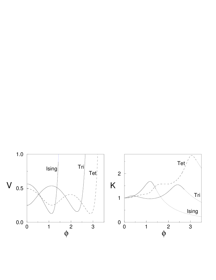
Figure 2: The potential $V(\varphi)$, and kinetic term coefficient function $K(\varphi)$, for the two dimensional Ising, tricritical Ising, and tetracritical Ising model fixed points.

Finally, what are the problems with this approach? The treatment of gauge theory present special problems: the formulation of a flow equation which properly treats the quantum aspects of gauge invariance non-perturbatively, and secondly, the construction of reliable approximations. The solution to the former must proceed in one of two ways: by allowing the cutoff to break the gauge invariance and then attempting to recover it as the cutoff is removed (via broken Ward identities),[32] or by generalizing the flow equations so that gauge invariance is not broken by the cutoff.[35] While the first method can be shown to work to all orders in perturbation theory,[33] it seems hopeless non-perturbatively.[34] It is surely through an exact preservation of the quantum gauge invariance that real progress will be made; a useable generalization of the pure $U(1)$ case [35] may well be possible. Note however, that for the interesting cases (non-Abelian and greater than two dimensions), derivative expansions per se are anyway impractical due to the large number of independent gauge invariant combinations that can be formed even at lowest non-trivial order.[35] Instead, much more appropriate forms of approximation deserve study in this case, such as large $N$ methods.

Returning to non-gauge theories, apart from the practical problem that higher orders in the derivative expansion get rapidly more complicated, one problem that this method shares with all other approximations to the renormalization group [4] is an unphysical dependence on the choice of cutoff function. This dependence is not really a problem however if instead it is used to estimate a rough lower bound on the error of the approximation, and thus test the numerical reliability.[20] For example, we can compare the $O(\partial^{0})$ $N=1$ results in table 1, to the corresponding results for sharp cutoff, $\nu=.70$ and $\omega=.60$.[13, 8] Another problem that has already been mentioned is that generically derivative expansions depend also on one unphysical parameter in the fixed point solutions, due to loss of reparametrization invariance. In a similar way this is not a problem (if one knows about it!), but rather can be used to test numerical reliability in such approximations.[8, 17] The real question that needs to be answered ultimately, is whether the derivative expansion exists to all orders and converges, because of course if it does, these problems have to lessen and eventually disappear as the expansion is pushed to higher orders. This question is hard to answer in generality, but rather straightforward to analyse perturbatively for a specific theory. In table 3, I show which results converge for the $\beta$ function of the $O(N)$ invariant scalar field theory in $D=4$ dimensions, computed to two loops with different forms of derivative expansion.[19] Also summarised are which expansions preserve reparametrization invariance.

Variant.	Repar. Inv.	Convergence.
		one loop	two loops
Wilson/Polchinski	X	X	X
Legendre Power	$\surd$	$\surd$	X
Legendre Faster	X	$\surd$	$\surd$
Legendre Sharp	$\surd$	$\surd$	$\surd$

Table 3: Properties of derivative expansions for different forms of flow equation and cutoff: Wilson or Polchinski flow equation with any smooth cutoff, Legendre flow equation with the Power law cutoff described in the text, Legendre flow equation with some Faster falling cutoffs, and momentum scale expansion of the Legendre flow equation with Sharp cutoff.

A direct derivative expansion of the Wilson effective action does not converge already at one loop: it is again a result of expansion of the propagators inside the effective action (mentioned earlier). On the other hand, the Legendre flow equations give the exact answer to the one loop $\beta$ function already at $O(\partial^{0})$.[2] Only the last two methods however converge at two loops. In particular, the sharp cutoff case converges very fast at two loops,[10] and since it also preserves a simple reparametrization invariance, further work to overcome the practical difficulties in its implementation [10] certainly seems called for. Although convergence even to all orders in perturbation theory, is no guarantee of convergence non-perturbatively (truncations in increasing powers of the field trivially must converge at any fixed order of perturbation theory, but as we have seen, fail to do so non-perturbatively), the natural conjecture is that these last two methods do converge non-perturbatively. The fact that the Legendre $O(\partial^{0})$ approximation is exact at $N=\infty$ [11, 23] lends further support to this conjecture.

Of course, negative answers to convergence do not exclude the first two methods from being good model approximations at low orders. Although I have concentrated on the Legendre flow equation with power law cutoff, derivative expansions of the Wilson / Polchinski equation are distinguished by their relative simplicity. Perhaps, by generalising the derivative expansion, one can preserve this simplicity while also preserving more of the structure of the exact renormalization group.

We remind that a large number of references to other work on the lowest order sharp cutoff approximation have been collected.[10] We collect here corresponding smooth cutoff versions not so far mentioned,[1, 36] and similarly attempts to go beyond leading order in the derivative expansion.[37] There are also a number of examples that entertain the idea of derivative expansion but in practice make further truncations.

In conclusion, the derivative (momentum scale) expansion methods – where no other approximation is made – are potentially very powerful, particularly in genuinely non-perturbative settings where all other methods fail. In contrast to more severe truncations, all these variants are robust, in the sense that no spurious solutions have been found, while especially the Legendre flow equation with power law cutoff yields very satisfactory numerical accuracy at low orders. The full potential of these methods is by no means yet realised, and much more theoretical progress on their properties is possible and expected.

References

References

- [1] K. Wilson and J. Kogut, Phys. Rep. 12C (1974) 75.
- [2] T.R. Morris, Int. J. Mod. Phys. A9 (1994) 2411.
- [3] T.R. Morris, Phys. Lett. B334 (1994) 355.
- [4] “Real-Space Renormalization” (1982), eds. T.W. Burkhardt and J.M.J. van Leeuwen, Springer, Berlin.
- [5] See particularly T.W. Burkhardt’s review.[4]
- [6] S.R. White, Phys. Rev. Lett. 69 (1992) 2863.
- [7] R.H. Swendsen’s review.[4]
- [8] T.R. Morris, Phys. Lett. B329 (1994) 241.
- [9] T.R. Morris, Phys. Lett. B345 (1995) 139.
- [10] T.R. Morris, Nucl. Phys. B458[FS] (1996) 477.
- [11] F.J. Wegner and A. Houghton, Phys. Rev. A8 (1973) 401.
- [12] J.F. Nicoll et al, Phys. Rev. Lett. 33 (1974) 540.
- [13] A. Hasenfratz and P. Hasenfratz, Nucl. Phys. B270 (1986) 687.
- [14] T.R. Morris, hep-th/9601128, to be published in Phys. Rev. Lett.
- [15] F.J. Wegner, J. Phys. C7 (1974) 2098; T.L. Bell and K.G. Wilson, Phys. Rev. B11 (1975) 3431;
- [16] E.K. Riedel, G.R. Golner and K.E. Newman, Ann.Phys. 161 (1985) 178.
- [17] G.R. Golner, Phys. Rev. B33 (1986) 7863.
- [18] J. Polchinski, Nucl. Phys. B231 (1984) 269.
- [19] T.R. Morris, in preparation.
- [20] See e.g. R.D. Ball et al, Phys. Lett. B347 (1995) 80.
- [21] J.F. Nicoll and T.S. Chang, Phys. Lett. 62A (1977) 287.
- [22] C. Wetterich, Phys. Lett. B301 (1993) 90.
- [23] T.R. Morris and M. Turner, in preparation.
- [24] J. Zinn-Justin, “Quantum Field Theory and Critical Phenomena” (1993) Clarendon Press, Oxford.
- [25] S. Ma, Phys. Rev. A10 (1974) 1818; Y. Okabe and M. Oku, Prog. Theor. Phys. 60 (1978) 1277.
- [26] K. Kanaya and S. Kaya, Phys. Rev. D51 (1995) 2404.
- [27] Such theories have been considered by J. Comellas, Y. Kubyshin and E. Moreno, hep-th/9512086, hep-th/9601112, and these proceedings.
- [28] A.B. Zamolodchikov, Yad. Fiz. 44 (1986) 821; J.L. Cardy, in “Phase Transitions and Critical Phenomena”, vol. 11 (1987), eds. C. Domb and J.L. Lebowitz, Academic Press.
- [29] P.S. Howe and P.C. West, Phys. Lett. B223 (1989) 371; M. Bauer, E. Brézin and C. Itzykson in “Statistical field theory”, vol. 1 (1989), C. Itzykson and J-M. Drouffe, CUP.
- [30] M. Asorey et al, hep-lat/9410009.
- [31] B. Schroer, Nucl. Phys. B295[FS21] (1988) 586.
- [32] U. Ellwanger, Phys. Lett. B335 (1994) 364.
- [33] M. Bonini, M. D’Attanasio and G. Marchesini, Nucl. Phys. B437 (1995) 163; Phys. Lett. B346 (1995) 87; M. Bonini, these proceedings.
- [34] M. D’Attanasio and T.R. Morris, Phys. Lett. B378 (1996) 213.
- [35] T.R. Morris, Phys. Lett. B357 (1995) 225.
- [36] A. Parola, J. Phys. C19 (1986) 5071; V.I. Tokar, Phys. Lett. A104 (1984) 135; G. Felder, Comm. Math. Phys. 111 (1987) 101; G. Zumbach, Nucl. Phys. B413 (1994) 754 and 771; A.E. Filippov and S.A. Breus, Phys. Lett. A158 (1991) 300, Physica A192 (1993) 486; A.E. Filippov, J. Stat. Phys. 75 (1994) 241.
- [37] G.R. Golner, Phys. Rev. B8 (1973) 339; A.E. Filippov and A.V. Radievsky, Phys. Lett. A169 (1992) 195.