Abstract

We study the properties of color-singlet Reggeon compound states in multicolor high-energy QCD in four dimensions. Their spectrum is governed by completely integrable (1+1)-dimensional effective QCD Hamiltonian whose diagonalization within the Bethe Ansatz leads to the Baxter equation for the Heisenberg spin magnet. We show that nonlinear WKB solution of the Baxter equation gives rise to the same integrable structures as appeared in the Seiberg-Witten solution for $N=2$ SUSY QCD and in the finite-gap solutions of the soliton equations. We explain the origin of hyperelliptic Riemann surfaces out of QCD in the Regge limit and discuss the meaning of the Whitham dynamics on the moduli space of quantum numbers of the Reggeon compound states, QCD Pomerons and Odderons.

Dedicated to the memory of Victor I. Ogievetsky

1. Introduction

In the last decades a tremendous progress has been achieved in understanding of low-dimensional integrable field theories and statistical models. Apart from the fact that their study serves as a laboratory for testing a new ideas, it has been expected for a long time that low-dimensional integrable systems should appear in the description of the effective dynamics of quantized (3+1)–dimensional Yang-Mills theories (see e.g. [1]). These expectations were confirmed in 1994 by two examples coming from different problems: the exact calculation of low-energy effective action of $N=2$ supersymmetric Yang-Mills theory [2] and study of the Regge asymptotics of perturbative QCD [3, 4]. It was found that well-known integrable structures emerge in both problems.

In the first example [2], the Seiberg–Witten solution for the low-energy effective action of pure $N=2$ SUSY Yang-Mills theory with the $SU(2)$ gauge group and its generalization to other gauge groups [5] were interpreted within the framework of finite-gap solutions of the soliton equations and their Whitham deformations [6]. In particular, the moduli space of vacua of $N=2$ SUSY $SU(N_{c})$ Yang-Mills theory without matter was identified as a moduli space of hyperelliptic curve $\Gamma$, which amazingly enough coincides with the spectral curve of 1-dimensional periodic Toda chain with $N_{c}$ sites [6, 7]. Moreover, including the matter hypermultiplets in the adjoint and fundamental representations leads to a deformation of the Toda spectral curve into the spectral curves corresponding to the Calogero-Moser integrable models [8, 9] and Heisenberg spin chains [10], respectively. The effective energy and the BPS spectrum of excitations can be expressed in terms of periods of a certain meromorphic 1-differential on $\Gamma$, which has a defining property that its external derivative is a holomorphic differential on $\Gamma$. This differential was identified as a generating functional of the Whitham equations describing the adiabatic deformations of soliton solutions [11]. There were different proposals to interpret the Whitham dynamics [6, 9, 12, 13] but, despite of a lot of efforts, the connection between integrable systems and the Seiberg-Witten solution still has a status of an observation and the underlying dynamical mechanism remains mysterious.

Our second example is related to the asymptotics of QCD at high energy and fixed transferred momentum, $s\gg-t$, the famous Regge limit [14]. It has been observed many years ago (see e.g. [15]) that perturbative expressions for the scattering amplitudes in QCD in the Regge limit have a striking similarity with predictions of a low-dimensional field theory. Indeed, it was realized that in the Regge limit QCD should be replaced by an effective $(2+1)-$dimensional Reggeon field theory [16], which should inherit all (still unknown) quantum symmetries of QCD. Recently, different attempts have been undertaken to deduce its effective action out of QCD [17, 18]. The resulting expressions become very complicated and the exact solution of the $S-$matrix of the Reggeon effective theory remains problematic. Nevertheless, there exists a meaningful approximation to the Reggeon effective theory, the so-called generalized leading logarithmic approximation (LLA) [19], in which the $S-$matrix of QCD exhibits remarkable properties of integrability. It turns out that in this approximation QCD is effectively described by the 1-dimensional quantum XXX Heisenberg magnet of spin $s=0$ [3, 4]. As a result, one can calculate the Regge asymptotics of the scattering amplitudes by applying a powerful Quantum Inverse Scattering Method [20]. In particular, the Bethe Ansatz solution of perturbative QCD $S-$matrix in the generalized LLA has been developed in [3, 21]. It is based on the Separation of Variables and leads to the Baxter equation for the XXX Heisenberg magnet [22, 23, 24].

The exact solution of the Baxter equation was established in a few special cases [3, 21] and different approaches to its general solution were proposed in [25, 26, 27, 28]. One of them is based on the quasiclassical expansion of the Baxter equation [26]. It allows to obtain asymptotic approximations to the solutions of the Baxter equation, which are in a good agreement with the results of numerical calculations.

In the present paper we continue the study of the Baxter equation started in [26]. We show that the WKB solution of the Baxter equation, describing the Regge limit of QCD, gives rise to the same integrable structures as appeared in the Seiberg-Witten solution for $N=2$ SUSY QCD and in the finite-gap solutions of the soliton equations. We explain the origin of hyperelliptic Riemann surfaces out of QCD in the Regge limit and discuss the meaning of Whitham dynamics on their moduli space.

The paper is organized as follows. In Sect. 2 we demonstrate the relation between high-energy QCD in the Regge limit and XXX Heisenberg magnet. The hamiltonian of the 1-dimensional XXX Heisenberg magnet appears as a kernel of the Bethe-Salpeter equation for the partial waves of the scattering amplitudes in multi-color QCD. Its diagonalization is performed in Sect. 3 by applying the method of Separation of Variables [22, 23, 24], which leads to the Baxter equation. In Sect. 4 we develop a nonlinear WKB expansion of the Baxter equation. We describe in detail the classical mechanics induced by the leading term of the WKB solution and establish a close relation between Reggeon compound states in QCD and soliton solutions of the KP/Toda hierarchy [29, 30]. The quantization conditions for the Reggeon compound states and their interpretation in terms of the Whitham flows are discussed in Sect. 5. The concluding remarks are summarized in Sect. 6.

2. High-energy QCD and Heisenberg spin magnet

Let us consider elastic hadron-hadron scattering in QCD at high energy, $s$, and fixed transferred momentum, $t$, and let us replace for simplicity nonperturbative hadronic states by perturbative onium states built from two heavy quarks with mass $M$. In this case, the scattering amplitude can be calculated in perturbative QCD as a sum of Feynman diagrams describing the multi-gluon exchanges between heavy quarks in the $t-$channel [31]. In the Regge limit, $s\gg-t\,,M^{2}$, the perturbative expressions for the Feynman diagrams involve large logarithmic corrections, $\alpha_{\rm s}^{n}\ln^{m}s$, which can be classified into the leading logs ($n=m$), next-to-leading logs ($n=m+1$) etc. and which have to be resummed to all orders in $\alpha_{\rm s}$. We recall, however, that one of the basic concepts of perturbative approach in QCD is that one considers quarks and gluons as elementary excitations and, assuming that their interaction is small, takes it into account as a perturbative expansion in $\alpha_{\rm s}$. The necessity of resuming perturbative series indicates that the description of a hadron-hadron scattering in terms of “bare” quarks and gluons is not appropriate anymore in the Regge limit and one has to identify instead a new collective degrees of freedom, in terms of which the QCD dynamics will be simpler.

In the Regge limit, due to remarkable property of the Reggeization in QCD [31], reggeized gluons, or Reggeons, become a new collective excitations. Although the Reggeon is built from an infinite number of “bare” gluons it behaves as a point-like particle. It carries the color charge of a gluon and it has a 4-momentum $k_{\mu}=(k_{+},k_{-},k_{\perp})$ with the longitudinal components $k_{\pm}$ belonging to the plane defined by the momenta of scattering hadrons and $k_{\perp}$ being 2-dimensional transverse momentum. The hadrons scatter each other by exchanging Reggeons in the $t-$channel and the interaction between Reggeons is described by the effective $S-$matrix, which should be obtained out of QCD in the Regge limit.

The Reggeon $S-$matrix has the following remarkable properties. Reggeons propagate in the $t-$channel between two hadrons and due to strong ordering of their longitudinal momenta the Reggeon rapidity $y=\ln\frac{k_{+}}{k_{-}}$ can be interpreted as a “time” in the $t-$channel [16]. Then, the Reggeon $S-$matrix describes the propagation of the Reggeons in the time $y$. Interacting with each other Reggeons change their 2-dimensional transverse momenta $k_{\perp}$ and color charge. Therefore, although Reggeons “live” in 4-dimensional Minkowski space-time, their $t-$channel evolution is described by the effective $(2+1)-$dimensional $S-$matrix [17, 18]. The exact expression for the Reggeon $S-$matrix is unknown yet and one may try to evaluate it in different approximations. In what follows we will study the Reggeon $S-$matrix in the generalized LLA [19]. In this approximation one preserves the unitarity of the $S-$matrix in the direct ($s-$, $t-$ and $u-$) channels but not in the subchannels.

2.1. Generalized LLA

The hadron-hadron (or onium-onium) scattering amplitude is given in the generalized LLA by the sum of effective Reggeon Feynman diagrams [19] in which, first, the number of Reggeons propagating in the $t-$channel is preserved (no creation/annihilation of Reggeons) and, second, only two Reggeons could interact with each other at the same moment of “time” $y$. Therefore, according to the number of Reggeons, $N$, the scattering amplitude can be decomposed as

$$A(s,t)=\sum_{N=2}^{\infty}\alpha_{\rm s}^{N-2}A_{N}(s,t)\,,$$

where the $N-$th term describes the evolution in the $t-$channel of the system of $N$ Reggeons with a pair-wise interaction. The amplitude $A_{N}(s,t)$ satisfies the Bartels-Kwiecinski-Praszalowicz equation [19], which can be interpreted as a Bethe-Salpeter equation for the $N$ Reggeon scattering amplitude. Its solutions define the color-singlet $N$ Reggeon compound states, perturbative QCD Pomerons and Odderons, whose contribution to the scattering amplitudes takes the standard Regge form

$$A_{N}(s,t)=is\sum_{\{q\}}\beta_{A}^{\{q\}}(t)\beta_{B}^{\{q\}}(t)\,s^{E_{N,\{q\}}}\,,$$

where indices $A$ and $B$ refer to the scattered hadrons. Here, $E_{N,\{q\}}$ is the energy of the $N$ Reggeon compound state. It is defined as an eigenvalue of the $N$ Reggeon hamiltonian

$${\cal H}_{N}|{\chi_{N,\{q\}}}\rangle=E_{N,\{q\}}|{\chi_{N,\{q\}}}\rangle\,,$$ (2.1)

with $\{q\}$ being some set of quantum numbers parameterizing all possible solutions. The residue functions $\beta_{A}^{\{q\}}$ and $\beta_{B}^{\{q\}}$ measure the overlapping between hadronic wave functions and the wave functions of the $N$ Reggeon compound states

$$\beta_{A}^{\{q\}}(t)=\langle{A|\chi_{N,\{q\}}}\rangle\,.$$

The pair-wise Reggeon hamiltonian ${\cal H}_{N}$ acts in (2.1) on 2-dimensional transverse momenta of $N$ Reggeons and the relation (2.1) has the form of a (2+1)–dimensional Schrödinger equation. Let us change the representation from 2–dimensional transverse Reggeon momenta space $k_{\perp}$ to 2-dimensional impact parameter space $b_{\perp}=(\xi,\zeta)$ and define the holomorphic and antiholomorphic complex coordinates of Reggeons as

$$z_{j}=\xi_{j}+i\zeta_{j}\,,\qquad\bar{z}_{j}=\xi_{j}-i\zeta_{j}\,,\qquad j=1,2,...,N\,.$$ (2.2)

Remarkable property of the Reggeon hamiltonian ${\cal H}_{N}$ is that being expressed in terms of holomorphic and antiholomorphic Reggeon coordinates, it splits in the multi-color limit, $\alpha_{\rm s}N_{c}=\mbox{fixed}$ and $N_{c}\to\infty$, into the sum of holomorphic and antiholomorphic hamiltonians [32]

$${\cal H}_{N}=\frac{\alpha_{\rm s}N_{c}}{4\pi}{\left({H_{N}+\overline{H}_{N}}\right)}+{\cal O}(N_{c}^{-2})\,,\qquad[H_{N},\overline{H}_{N}]=0\,,$$

where $H_{N}$ and $\overline{H}_{N}$ act on holomorphic and antiholomorphic Reggeon coordinates, respectively. Since the hamiltonians $H_{N}$ and $\overline{H}_{N}$ commute with each other, the original (2+1)–dimensional Schrödinger equation (2.1) can be replaced by the system of holomorphic and antiholomorphic (1+1)–dimensional Schrödinger equations

$$H_{N}|{\varphi_{N,\{q\}}}\rangle=\varepsilon_{N,\{q\}}|{\varphi_{N,\{q\}}}\rangle\,,\qquad\overline{H}_{N}|{\overline{\varphi}_{N,\{q\}}}\rangle=\overline{\varepsilon}_{N,\{q\}}|{\overline{\varphi}_{N,\{q\}}}\rangle\,,$$ (2.3)

which define the spectrum of the Reggeon compound states as follows

$$E_{N,\{q\}}=\frac{\alpha_{\rm s}N_{c}}{4\pi}{\left({\varepsilon_{N,\{q\}}+\overline{\varepsilon}_{N,\{q\}}}\right)}\,,\qquad\chi_{N,\{q\}}(z,\bar{z})=\varphi_{N,\{q\}}(z)\,\overline{\varphi}_{N,\{q\}}(\bar{z})\,,$$ (2.4)

where $z$ and $\bar{z}$ denote the full set of $N$ Reggeon holomorphic and antiholomorphic coordinates. Thus, in the generalized LLA perturbative (3+1)–dimensional multi-color QCD is effectively replaced by the system of (1+1)–dimensional Schrödinger equations (2.3). The properties of two equations in (2.3) are similar and in what follows we will study only the holomorphic Schrödinger equation in (2.3) for fixed number of Reggeons $N$.

2.2. Integrability

The holomorphic hamiltonian $H_{N}$ describes the nearest-neighbour interaction between $N$ Reggeons with holomorphic coordinates $z_{1}$, $...$, $z_{N}$ and periodic boundary conditions $z_{k+N}=z_{k}$

$$H_{N}=\sum_{j=1}^{N+1}H_{j,j+1}$$ (2.5)

and $H_{N,N+1}=H_{N,1}$. Here, the interaction hamiltonian between two Reggeons, $H_{j,j+1}$, is given by the BFKL kernel [31, 33]

$$H_{12}\equiv H(z_{1},z_{2})=-\psi(-J_{12})-\psi(1+J_{12})+2\psi(1)\,,$$ (2.6)

where $\psi(x)=\frac{d\ln\Gamma(x)}{dx}$ and the operator $J_{12}$ is defined as an operator solution of the equation

$$J_{12}(1+J_{12})=-(z_{1}-z_{2})^{2}\partial_{1}\partial_{2}$$

with $\partial_{k}=\partial/\partial z_{k}$. We stress that the operator (2.6) was originally derived [31] from the analysis of Feynman diagrams contributing to the Regge asymptotics of the onium-onium scattering amplitude in perturbative QCD. Therefore, it was quite unexpected to find [3, 4] that it coincides with the hamiltonian of 1-dimensional XXX Heisenberg magnet of spin $s=0$ corresponding to the principal series representation of the $SL(2,\hbox{$\,\vrule height=6.45831pt,width=0.4pt,depth=0.0pt\kern-3.00003pt{\rm C}$})$ group. The number of sites of the spin chain is equal to the number of Reggeons.

Among other things this equivalence means that the holomorphic Schrödinger equation (2.3) possesses the family of hidden mutually commuting conserved charges [3, 4]

$$[q_{k},q_{j}]=[q_{k},H_{N}]=0$$ (2.7)

and their number is large enough for the system (2.3) to be completely integrable. To identify the conservation laws for the system of $N$ interacting Reggeons one applies the Quantum Inverse Scattering Method [20] and uses well-known constructions for the Heisenberg magnet [34, 35]. Namely, to each Reggeon we assign the (auxiliary) Lax operator

$$L_{k}=\left(\begin{array}[]{cc}\lambda+iS_{k}^{3}&iS_{k}^{-}\\ iS_{k}^{+}&\lambda-iS_{k}^{3}\end{array}\right)=\lambda\cdot\hbox{{1}\kern-2.5pt\hbox{l}}+i\left({1\atop z_{k}}\right)\otimes(z_{k},-1)\partial_{k}\,,$$ (2.8)

where $\lambda$ is an arbitrary complex parameter and $S_{k}^{\alpha}$ are spin $s=0$ generators of the $SL(2)$ group acting on the holomorphic coordinates of the $k-$th Reggeon

$$S_{k}^{3}=z_{k}\partial_{k}\,,\qquad S_{k}^{+}=z_{k}^{2}\partial_{k}\,,\qquad S_{k}^{-}=-\partial_{k}\,.$$

Then, we construct the monodromy matrix

$$T(\lambda)=L_{N}(\lambda)L_{N-1}(\lambda)...L_{1}(\lambda)=\left(\begin{array}[]{cc}A(\lambda)&B(\lambda)\\ C(\lambda)&D(\lambda)\end{array}\right)\,,$$ (2.9)

where the operators $A$, $B$, $C$ and $D$ act on the holomorphic coordinates of $N$ Reggeons and satisfy the Yang-Baxter equation [35, 34]. Finally, we obtain the transfer matrix as

$$\Lambda(\lambda)=\mbox{tr\,}T(\lambda)=A(\lambda)+D(\lambda)$$ (2.10)

and verify, using (2.8) and (2.9), that $\Lambda(\lambda)$ is a polynomial of the degree $N$ in $\lambda$

$$\Lambda(\lambda)=2\lambda^{N}+q_{2}\lambda^{N-2}+...+q_{N}\,,$$ (2.11)

with the coefficients $q_{k}$ being operators acting on holomorphic coordinates of the Reggeons. It immediately follows from the Yang-Baxter equation for the monodromy matrix $T(\lambda)$ that the operators $q_{2}$, $...$, $q_{N}$ satisfy the relations (2.7) .

Thus, we identify the operators $q_{2}$, $...$, $q_{N}$ as $N-1$ conserved charges for the system of $N$ interacting Reggeons. To match the number of conservation laws with the number of Reggeons, one needs one more conserved charge. It is easy to see that the remaining $N-$th charge is associated with the center-of-mass motion of the $N$ Reggeon compound state and it is equal to the total Reggeon momentum

$$P=\pi_{1}+\pi_{2}+...+\pi_{N}=i(S^{-}_{1}+S^{-}_{2}+...+S^{-}_{N})$$

with $\pi_{j}=-i\partial_{j}$ being the holomorphic component of 2-dimensional transverse momentum of the $j-$th Reggeon. The explicit expressions for the operators $q_{k}$ can be obtained from (2.8), (2.9) and (2.11) as [3, 4]

$$q_{k}=\sum_{N\geq j_{1}>j_{2}>...>j_{k}\geq 1}i^{k}z_{j_{1}j_{2}}z_{j_{2}j_{3}}...z_{j_{k}j_{1}}\partial_{j_{1}}\partial_{j_{2}}...\partial_{j_{k}}$$ (2.12)

with $z_{jk}=z_{j}-z_{k}$. They can be interpreted as higher Casimir operators of the $SL(2)$ group and their appearance can be traced back to the invariance of the Reggeon hamiltonian (2.5) under the Möbius transformations

$$z_{k}\to\frac{az_{k}+b}{cz_{k}+d}\,,$$ (2.13)

where $ac-bd=1$. In particular,

$$q_{2}=\sum_{N\geq j>k\geq 1}z_{jk}^{2}\partial_{j}\partial_{k}=-h(h-1)$$ (2.14)

is the quadratic Casimir operator and its eigenvalue $h$ defines the conformal weight of the holomorphic wave function $\varphi_{N}(z_{1},...,z_{N})$ of the $N$ Reggeon compound state (2.4). The Reggeon wave function belongs to the principal series representation of the $SL(2,\hbox{$\,\vrule height=6.45831pt,width=0.4pt,depth=0.0pt\kern-3.00003pt{\rm C}$})$ group and, as a result, its conformal weight is quantized

$$h=\frac{1+m}{2}+i\nu,\,,\qquad m=\mathchoice{\hbox{\cmss Z\kern-3.99994ptZ}}{\hbox{\cmss Z\kern-3.99994ptZ}}{\lower 0.9pt\hbox{\cmsss Z\kern-4.39993ptZ}}{\lower 1.2pt\hbox{\cmsss Z\kern-4.39993ptZ}}\,,\quad\nu={\hbox{{\rm I}\kern-1.99997pt\hbox{\rm R}}}\,.$$ (2.15)

Here, integer $m$ defines the Lorentz spin of the Reggeon state (2.4), corresponding to the rotations in the 2-dimensional impact parameter space, $\chi_{N}\to\mbox{e}^{im\alpha}\chi_{N}$ as $z_{j}\to\mbox{e}^{i\alpha}z_{j}$ and $\bar{z}_{j}\to\mbox{e}^{-i\alpha}\bar{z}_{j}$. The quantization conditions for the remaining charges $q_{3}$, $...$, $q_{N}$ are much more involved [26] and their interpretation in terms of the properties of Reggeon states will be given in Sect. 5.

Once we identified the complete set of conservation laws, the Reggeon hamiltonian becomes a rather complicated function of the conserved charges , $H_{N}=H_{N}(q_{2},...,q_{N})$, and one can replace the original Schrödinger equation (2.3) by a simpler problem of simultaneous diagonalization of the operators $P$, $q_{2}$, $...$, $q_{N}$. Their eigenvalues form a complete set of quantum numbers parameterizing the $N$ Reggeon compound states, $\varphi_{N,\{q\}}(z_{1},...,z_{N})$.

3. Separation of variables

Diagonalization of the conserved charges can be performed using the Separation of Variables (SoV) [22, 23, 24]. The operators $P$, $q_{2}$, $...$, $q_{N}$ depend on the coordinates and momenta, $z_{k}$ and $\pi_{k}=-i\partial_{k}$, respectively, of $N$ Reggeons and their diagonalization is reduced to solving of a complicated system of $N$ coupled partial differential equations for the holomorphic wave function of the $N$ Reggeon state. Instead of dealing with this system we perform a unitary transformation

$$(z_{j},\pi_{j})\to(x_{j}=U^{\dagger}z_{j}U,p_{j}=U^{\dagger}\pi_{j}U)\,,\qquad U=U(\{z_{k},\pi_{k}\})$$ (3.1)

in order to replace the original set of Reggeon coordinates and momenta, $(z_{j},\pi_{j})$, by a new canonical set of separated variables

$$[x_{j},x_{k}]=[p_{j},p_{k}]=0\,,\qquad[p_{j},x_{k}]=-i\delta_{jk}\,,$$ (3.2)

in terms of which the following relations hold

$$\Phi(x_{j},p_{j};q_{2},...,q_{N})|{\varphi_{N,\{q\}}}\rangle = 0\,,\quad j=1,2,...,N-1\,,$$ (3.3)

$$(p_{N}-P)|{\varphi_{N,\{q\}}}\rangle = 0\,.$$

Here, the number of pairs $(x_{j},p_{j})$ is equal to the number of Reggeons, $N$. One of the pairs, $(x_{N},p_{N})$, describes the center-of-mass motion of the $N$ Reggeon state

$$x_{N}=\frac{1}{N}{\sum_{j=1}^{N}z_{j}}\,,\qquad p_{N}=\sum_{j=1}^{N}\pi_{j}\,,$$ (3.4)

while the definition of the remaining separated coordinates and the functions $\Phi$ will be given below. In relation (3.3), the operators are ordered inside the function $\Phi$ as they are enlisted and the conserved charges $q_{k}$ can be replaced by their eigenvalues corresponding to the $N$ Reggeon compound state $\varphi_{N,\{q\}}$.

The remarkable property of the separated coordinates is that in the $x-$representation, $p_{j}=-i\partial/\partial x_{j}$, the relations (3.3) define the system of $N$ separated differential equations for the wave function of the $N$ Reggeon state $\varphi_{N,\{q\}}=\varphi_{N,\{q\}}(x_{1},...,x_{N})$ and its solution takes the following factorized form

$$\varphi_{N,\{q\}}(x_{1},...,x_{N})=Q(x_{1})Q(x_{2})...Q(x_{N-1})\exp(iPx_{N})\,,$$ (3.5)

where $P$ is the total momentum of the state and a function $Q(x)$ satisfies the Baxter equation

$$\Phi(x,-i\partial_{x};q_{2},...,q_{N})Q(x)=0\,.$$ (3.6)

To obtain the wave function in terms of the holomorphic Reggeon coordinates one has to go back from $x-$ to $z-$representation in (3.1) by applying the unitary transformation $U$. The resulting expression can be found in [3].

3.1. Baxter equation

Let us construct the separated variables for the system of $N$ Reggeons. Before doing this we would like to notice that the SoV method has been extensively developed in application to 1-dimensional classical integrable systems. In this case, as it was shown in many examples [29], poles of a properly normalized Baker-Akhiezer function provide the set of separated coordinates. Having expressions for the separated variables in the classical system, one may try to generalize them to the corresponding quantum integrable model. However, one of the peculiar features of the holomorphic Schrödinger equation for the $N$ Reggeon compound states is that it describes 1-dimensional essentially quantum integrable system and one has to determine the separated variables without knowing their classical analogs.

Constructing the separated variables for the $N$ Reggeon state we follow the approach developed by Sklyanin [24]. Namely, we define the separated coordinates $x_{1}$, $...$, $x_{N-1}$ as operator zeros of the operator $B(\lambda)$ entering the expression (2.9) for the monodromy matrix. According to (2.8) and (2.9), $B(\lambda)$ is a polynomial of the degree $N-1$ in $\lambda$ and it can be represented as

$$B(\lambda)=p_{N}(\lambda-x_{1})(\lambda-x_{2})...(\lambda-x_{N-1})\,,$$

where $p_{N}$ was defined in (3.4) and the ordering of operators is unessential due to (3.2). The definition of the momenta $p_{j}$ conjugated to the coordinates $x_{j}$ takes a few steps. Let us substitute $\lambda=x_{j}$ into (2.9). Since the operators $A(\lambda)$, $C(\lambda)$ and $D(\lambda)$ do not commute with $x_{j}$ we use the prescription of “substitution from the left”, $\lambda\mapsto x_{j}$. This means [24], that for an arbitrary operator $W(\lambda)=\sum_{k}\lambda^{k}W_{k}$ one first pulls out all powers of $\lambda$ to the left and then replaces $\lambda$ by the operator $x_{j}$ as $W{\left({\lambda\mapsto x_{j}}\right)}=\sum_{k}x_{j}^{k}W_{k}$. For $\lambda\mapsto x_{j}$ the monodromy matrix (2.9) takes a triangle form with the diagonal elements given by

$$A{\left({\lambda\mapsto x_{j}}\right)}=x_{j}^{N}\omega_{j}^{+}\,,\qquad D{\left({\lambda\mapsto x_{j}}\right)}=x_{j}^{N}\omega_{j}^{-}\,,$$ (3.7)

where notation was introduced for the operators $\omega_{j}^{+}$ and $\omega_{j}^{-}$.

Let us forget for a moment that we are dealing with operators and replace all operators by the corresponding classical functions. Then, one could identify the diagonal elements $x_{j}^{N}\omega_{j}^{\pm}$ of the monodromy matrix $T(\lambda)$ as its eigenvalues and write down the characteristic equation for $\omega^{\pm}$ as

$$\det(T(x)-x^{N}\omega)=x^{2N}\omega^{2}-x^{N}\omega\ \mbox{tr\,}T(x)+\det T(x)=0\,.$$

Using the definition of the transfer matrix, (2.10), and that classically $\det T(\lambda)=\prod_{k=1}^{N}\det L_{k}(\lambda)$ $=\lambda^{2N}$ we obtain the relation

$$\omega+\frac{1}{\omega}=x^{-N}\Lambda(x)=2+\frac{q_{2}}{x^{2}}+...+\frac{q_{N}}{x^{N}}\,,$$ (3.8)

which can be interpreted as the level surface of the commuting integrals of motion $q_{k}$, or spectral curve of the monodromy operator for some classical Liouville integrable system [29]. As we will show in the next section, this system arises as a quasiclassical limit of the $N$ Reggeon state.

Let us take now into account noncommutativity of operators and establish the quantum analog of the spectral curve (3.8). Using the Yang-Baxter equation for the monodromy matrix (2.9) one can verify the following relations for the operators $\omega^{\pm}_{k}$ [24]

$$[\omega_{j}^{\pm},\omega_{k}^{\pm}]=[\omega_{j}^{\pm},\omega_{k}^{\mp}]=0\,,\qquad\omega_{j}^{+}\omega_{j}^{-}=1\,,\qquad\omega_{j}^{\pm}x_{k}=(x_{k}\pm i\delta_{jk})\omega_{j}^{\pm}\,.$$

These relations suggest that the operators $\omega^{\pm}_{j}$ act on the Reggeon wave function in the $x-$representation as shift operators and they allow us to define the momentum $p_{j}$ conjugated to $x_{j}$ in the separated variables as follows

$$\omega_{j}\equiv\omega_{j}^{+}=\frac{1}{\omega_{j}^{-}}=\pm\exp(-p_{j})\,,\qquad\omega_{k}Q(x_{j})=\pm Q(x_{j}+i\delta_{jk})\,.$$ (3.9)

We notice that the canonical commutation relations (3.2) do not allow to fix a sign ambiguity in the definition of the momentum.

To establish the relations (3.3) in the separated variables $(x_{j},p_{j})$, we substitute $\lambda\mapsto x_{j}$ into the definition (2.10) of the transfer matrix and use (3.7) to get

$$\omega_{j}+\frac{1}{\omega_{j}}=x_{j}^{-N}\Lambda(x_{j})=2+x_{j}^{-2}q_{2}+...+x_{j}^{-N}q_{N}\,,\qquad$$ (3.10)

where $j=1$, $...$, $N-1$ and the ordering of the operators $x_{j}$ and $q_{k}$ is important since they do not commute with each other. The operator identity (3.10) can be considered as a quantum analog of the spectral curve (3.8). It relates a pair of the separated variables $(x_{j},p_{j})$ to the set of the conserved charges and being applied to the wave function of the $N$ Reggeon compound state it leads to (3.3), provided that

$$\Phi(x_{j},p_{j};q_{2},...,q_{N})=x_{j}^{-N}\Lambda(x_{j})-2\cosh p_{j}\,.$$ (3.11)

Here, we used (3.9) with a plus sign and took into account the possibility to change a sign by introducing an ambiguity $p_{j}\to p_{j}+i\pi$ in the definition of the momentum. Substituting (3.11) into (3.6) we find that the wave function $Q(x_{j})$ satisfies the finite-difference equation

$$x_{j}^{-N}\Lambda(x_{j})\,Q(x_{j})=Q(x_{j}+i)+Q(x_{j}-i)\,,\qquad j=1,2,...,N-1\,,$$ (3.12)

which has the same form as the equation for eigenvalues of the Baxter $Q-$operator [37]. In this equation, $x_{j}$ denotes the eigenvalue of the corresponding coordinate operator. Notice that the operators $q_{k}$ entering into the definition of the transfer matrix (2.11) have been replaced in (3.12) by their eigenvalues corresponding to the $N$ Reggeon compound state. As for any quantum system, the possible values of $q_{k}$ are constrained by the quantization conditions which will be discussed below.

Having solved the Baxter equation (3.12), one can obtain the wave function of the $N$ Reggeon compound state (3.5). Moreover, the same function $Q(x)$ controls the dependence of the holomorphic Reggeon hamiltonian on the conserved charges and for a given set of quantum numbers $q_{2}$, $...$, $q_{N}$ the holomorphic energy of the $N$ Reggeon state, defined in (2.3), can be evaluated as [3, 21]

$$\varepsilon_{N}(q_{2},...,q_{N})=i\frac{d}{dx}\ln\frac{Q(x-i)}{Q(x+i)}\bigg{|}_{x=0}\,.$$ (3.13)

The Baxter equation (3.12) alone does not allow us to find its solution $Q(x)$. One has to specify additionally the spectrum of the operators $x_{1}$, $...$, $x_{N}$ and provide the appropriate boundary conditions for the function $Q(x)$. It is clear that the possible eigenvalues of the coordinate operators $x_{k}$ depend on the class of functions $Q(x)$ on which they act. For example, the spectrum of $x_{j}$ is discrete for the spin$-\frac{1}{2}$ Heisenberg magnet, while for the Toda chain the eigenvalues of $x_{j}$ take continuous real values [22, 23, 24]. To find the spectrum of the operators $x_{j}$ for the Reggeon states we have to impose additional conditions on the functions $Q(x)$. To this end we notice that the solution of the Baxter equation $Q(x)$ defines the wave function of the Reggeon compound state (3.5) and the above conditions should follow from the requirement for its norm to be finite. Although the explicit expression for the norm is known [3, 4], the general form of the resulting constraints on the functions $Q(x)$ was not found yet, except of the subclass of the so-called polynomial solutions of the Baxter equation [26], corresponding to the special values of quantized conformal weight (2.15).

3.2. Polynomial solutions of the Baxter equation

The subclass of polynomial solutions covers all normalizable solutions of the Baxter equation corresponding to the integer positive conformal weight of the $N$ Reggeon compound states

$$h=\mathchoice{\hbox{\cmss Z\kern-3.99994ptZ}}{\hbox{\cmss Z\kern-3.99994ptZ}}{\lower 0.9pt\hbox{\cmsss Z\kern-4.39993ptZ}}{\lower 1.2pt\hbox{\cmsss Z\kern-4.39993ptZ}}_{+}\,,\qquad h\geq N\,,$$ (3.14)

where one put $\nu=0$ and $m\geq 2N-1$ to be odd in (2.15). In this case, as was shown in [26], the normalizable solutions $Q(x)$ of the Baxter equation become polynomials of the degree $h$ in $x$ with $N$ time degenerate root $x=0$

$$Q(x)=x^{N}\prod_{j=1}^{h-N}(x-\lambda_{j})\,.$$ (3.15)

Each solution is characterized by the set of nonvanishing roots $\{\lambda_{j}\}$. Having the explicit expressions for the roots, one can easily evaluate from (3.12) and (3.13) the quantum numbers $q_{k}$ and the corresponding energy of the $N$ Reggeon states. It follows from the Baxter equation (3.12) that $\lambda_{j}$ satisfy the Bethe equations for the XXX magnet of spin $s=0$ [21]. Their study reveals the following interesting properties of the polynomial solutions of the Baxter equation [21, 26].

For any given integer $h$ in (3.14), the space of polynomial solutions is finite-dimensional. The possible values of roots $\lambda_{k}$, as well as the values of quantized $q_{k}$ and the energy $\varepsilon_{N}$, turn out to be real and simple

$$\hbox{\rm Im}\,\lambda_{j}=\hbox{\rm Im}\,q_{k}=\hbox{\rm Im}\,\varepsilon_{N}=0$$ (3.16)

and they can be parameterized by integers $n_{1}$, $...$, $n_{N-2}$

$$q_{k}=q_{k}(h;n_{1},...,n_{N-2})\,,\qquad\varepsilon_{N}=\varepsilon_{N}(h;n_{1},...,n_{N-2})$$ (3.17)

such that

$$n_{1},...,n_{N-2}\geq 0\,,\qquad\sum_{k=1}^{N-2}n_{k}\leq h-N\,.$$

The eigenvalues of the coordinate operators $x_{1}$, $...$, $x_{N-1}$ are also real for the polynomial solutions and they occupy $N-1$ compact nonoverlapping intervals on the real axis

$$\hbox{\rm Im}\,x_{j}=0\,,\qquad x_{j}\in[\sigma_{2j-1},\sigma_{2j}]\,.$$ (3.18)

The positions of the intervals, $\sigma_{k}$, depend on the values of quantized $q_{3}$, $...$, $q_{N}$ and they satisfy the following relation

$$\Lambda^{2}(\sigma_{k})=4\sigma_{k}^{2N}\,.$$ (3.19)

The possible values of roots $\lambda_{k}$ belong to the same intervals (3.18) and their distribution on the real axis was found in the limit of large integer conformal weight, $h\gg 1$. Moreover, in the large $h$ limit the following scaling holds

$$\lambda_{j}={\cal O}(h)\,,\qquad q_{2}={\cal O}(h^{2})\,,\ ...\ ,\ q_{N}={\cal O}(h^{N})\,,\ \ \ \varepsilon_{N}={\cal O}(\ln h)\,,$$ (3.20)

which allows to develop the asymptotic expansion of $q_{k}$ and $\varepsilon_{N}$ in inverse powers of the conformal weight

$$q_{k}=h^{k}\sum_{l=0}^{\infty}q_{k}^{(l)}(n)\,h^{-l}\,,\qquad\varepsilon_{N}=-2N\ln h+\sum_{l=0}^{\infty}\varepsilon_{N}^{(l)}(n)\,h^{-l}\,.$$ (3.21)

where $k=3$, $...$, $N$ and the coefficients $q_{k}^{(l)}$ and $\varepsilon_{N}^{(l)}$ depend on the integers $n_{k}$. For $N=2$ Reggeon states all coefficients are known exactly and for $N=3$ Reggeon states they were calculated up to ${\cal O}(h^{-8})$ order [26].

Comparing the asymptotic expansions (3.21) for $N=2$ and $N\geq 3$ Reggeon states one can discover two important differences [26]. First, the coefficients $\varepsilon_{N}^{(l)}$ grow as factorials to higher orders in $1/h$. The asymptotic series for the energy of $N=2$ Reggeon states is Borel summable, but for $N\geq 3$ the properties of the same series are drastically changed and it becomes non Borel summable. Second, for $N\geq 3$ Reggeon states one has to study additionally the properties of the “higher” quantum numbers $q_{3}$, $...$, $q_{N}$. One finds that for $N\geq 3$ Baxter equation among all possible polynomial solutions there are a few singular solutions, corresponding to the situation, when either one of the intervals (3.18) is shrinking into a point, or two intervals merge, $\sigma_{j-1}=\sigma_{j}$. On the quantum moduli space of $q_{3}$, $...$, $q_{N}$ the singular solutions are described by the “critical” $(N-3)-$dimensional hypersurface

$$\Sigma_{N}(q_{3}^{\rm crit},...,q_{N}^{\rm crit})=0\,.$$ (3.22)

For example, for $N=3$ Reggeon states the critical values of $q_{3}$ are just three points given by

$$q_{3}^{\rm crit}=0\quad\mbox{and}\quad\pm\frac{h^{3}}{\sqrt{27}}{\left({1+{\cal O}(h^{-1})}\right)}\,.$$ (3.23)

As we will show in Sect. 4, both properties are closely related to each other and they can be simply understood using the properties of hyperelliptic Riemann surfaces determined by the complex curve (3.8).

The polynomial solutions of the Baxter equation are closely related to the different systems of orthogonal polynomials [21]. For $N=2$ the exact solution of the Baxter equation was identified as a continuous Hahn symmetric polynomial. For $N\geq 3$ more complicated systems of orthogonal polynomials arise and their properties can be studied using the approach developed in [38].

3.3. Quasiclassical limit

The derivation of the Baxter equation in Sect. 3.1 was based on the close relation between Heisenberg spin magnet and the system of $N$ interacting Reggeons in multi–color QCD. It is not surprising therefore that similar equations appear in different 1-dimensional quantum integrable systems. Namely, applying the SoV to the periodic Toda chain with $N$ sites one obtains the Baxter equation in the form [23, 24, 39]

$$\Lambda_{\rm Toda}(x_{j})\,Q(x_{j})=Q(x_{j}+i\hbar)+Q(x_{j}-i\hbar)\,,\qquad j=1,2,...,N-1\,,$$ (3.24)

where $\Lambda_{\rm Toda}$ is the corresponding transfer matrix and $\hbar$ is the Planck constant. Comparing (3.12) and (3.24) we notice a trivial but important difference between two models – the Baxter equation for the $N$ Reggeon state, as well as the canonical commutation relations (3.2), do not involve the Planck constant. Indeed, the Planck constant enters into the definition of the XXX Heisenberg magnet as a coefficient in front of the second term in the Lax operator (2.8). The Reggeon Lax operator (2.8) and, as a consequence, the Baxter equation (3.12) correspond to the special case $\hbar=1$.

Thus, the system of $N$ Reggeons does not have any natural small parameter, which would allow us to perform the quasiclassical limit, $Q(x)=\exp(\frac{i}{\hbar}S(x))$ as $\hbar\to 0$, and obtain its classical integrable analog. Nevertheless, there is a simple way of introducing a small parameter $\eta$ into the Baxter equation similar to the one used in asymptotic solutions of the Painlevé type I equation [40]. Let us rescale in (3.12) the collective coordinate as $x\to x/\eta$ and introduce notations

$$f(x)=\eta^{h}Q(x/\eta)\,,\qquad\hat{q}_{k}=q_{k}\eta^{k}\,.$$ (3.25)

Then, one could identically rewrite the Baxter equation (3.12) as

$$f(x+i\eta)+f(x-i\eta)=x^{-N}\Lambda(x,\{\hat{q}_{k}\})f(x)\,,$$ (3.26)

where the transfer matrix is given by (2.11) with $q_{k}$ replaced by $\hat{q}_{k}$ defined in (3.25). Following [40], let us look for the solutions of the Baxter equation in the form

$$f(x)=\exp{\left({\frac{i}{\eta}S(x,\{\hat{q}_{k}\})}\right)}\,,\qquad S(x,\{\hat{q}_{k}\})=S_{0}(x)+\eta S_{1}(x)+...\ ,$$ (3.27)

where each term is assumed to be uniformly bounded and the expansion to be convergent.

The asymptotic expansion (3.27) of the solutions of the Baxter equation naturally appears in the limit $\eta\to 0$ and $\hat{q}_{k}=\mbox{fixed}$. According to (3.25) and (2.14), this limit corresponds to the large values of the conformal weight, $h\sim 1/\eta\to\infty$, and it was studied in [26]. Using (3.15), (3.25) and (3.27) we can express $S$ in terms of the roots $\lambda_{j}$ as

$$S(x;\{\hat{q}_{k}\})=-i\eta\sum_{j=1}^{h}\ln(x-\lambda_{j}\eta)\,,$$ (3.28)

where $\lambda_{h-N+1}=...=\lambda_{h}=0$. Then, for $h\sim 1/\eta\to\infty$ the property of roots (3.20) implies the scaling $\lambda_{j}\eta={\cal O}(\eta^{0})$ and $S(x;\{\hat{q}_{k}\})={\cal O}(\eta^{0})$, which leads to the asymptotic expansion (3.27).

Substituting the ansatz (3.27) into (3.26) and expanding the both sides of the Baxter equation (3.26) to order $\eta$ one obtains [39]

$$2\cosh S_{0}^{\prime}(x)=x^{-N}\Lambda(x;\{\hat{q}_{k}\})\,,\qquad S_{1}^{\prime}(x)=\frac{i}{2}S_{0}^{\prime\prime}(x)\coth S_{0}^{\prime}(x)\,,$$ (3.29)

where prime denotes a derivative with respect to $x$. Then, the solution of the Baxter equation (3.26) is given by

$$f(x)=\frac{1}{\left[\sinh S_{0}^{\prime}(x)\right]^{1/2}}\exp{\left({\frac{i}{\eta}\int^{x}dS_{0}(x)+{\cal O}(\eta)}\right)}\,.$$ (3.30)

Comparing (3.26) with the Baxter equation for the Toda chain (3.24) we observe that the parameter $\eta$ plays a role of the Planck constant. The ansatz (3.30) takes the form of the WKB expansion with the leading term $S_{0}(x)$ being the “Reggeon classical action”. Let us study the classical mechanics of the $N$ Reggeon system governed by the action $S_{0}(x)$.

4. Quasiclassical Reggeon states as KP/Toda solitons

Let us introduce notation for the function

$$\omega(x)=\exp(S_{0}^{\prime}(x))$$ (4.1)

and rewrite the first equation in (3.29) as

$$\omega+\frac{1}{\omega}=x^{-N}\Lambda(x;\{\hat{q}_{k}\})\,.$$ (4.2)

This expression is the quasiclassical analog of the operator relation (3.10). We notice that the variable $x$ appears in (3.26) and (4.2) as a collective coordinate of the Reggeons and for polynomial solutions it takes values inside one of the $N-1$ compact intervals on the real axis (3.18). The classical analog of the Reggeon momentum in the separated coordinates, $[x,p]=i\eta$, can be obtained from (3.9) as

$$p=\ln|\omega(x)|\,,$$ (4.3)

where $\omega$ takes positive and negative values in (4.2) and the modulus is needed for momentum $p$ to be real. Using (4.2) and taking into account that $\omega$ is real on the classical trajectories, we obtain the relations which define the intervals of the classical motion of Reggeons as

$$\Lambda^{2}(x_{j};\{\hat{q}_{k}\})\geq 4x_{j}^{2N}\,,\qquad j=1,2,...,N-1\,,$$ (4.4)

where index refers to the $j-$th allowed band. This relation is in agreement with (3.19).

4.1. Spectral curve

Let us continue the relation (4.2) into the complex domain. For $\eta=1$ it coincides with the spectral curve (3.8) and replacing

$$y=x^{N}{\left({\omega-\frac{1}{\omega}}\right)}$$ (4.5)

one can rewrite it in the conventional form as

$$\Gamma_{N}:\qquad y^{2}=\Lambda^{2}(x)-4x^{2N}=4\hat{q}_{2}P_{2N-2}(x)$$ (4.6)

where $P_{2N-2}(x)=x^{2N-2}+...\$ is a polynomial with the coefficients depending on the quantum numbers $\hat{q}_{k}$ of the $N$ Reggeon state. The curve (4.6) determines the hyperelliptic Riemann surface $\Gamma_{N}$ equipped with a meromorphic differential $dS_{0}$ defined in (3.29). The genus of the Riemann surface, $g=N-2$, depends on the number of Reggeons inside the compound state. For $N=2$ Reggeon state, the well-known BFKL Pomeron [31], $\Gamma_{2}$ is a sphere,

$$\Gamma_{2}:\qquad y^{2}=\hat{q}_{2}(4x^{2}+\hat{q}_{2})$$ (4.7)

while for $N=3$ Reggeon state, the QCD Odderon [41], $\Gamma_{3}$ is a torus,

$$\Gamma_{3}:\qquad y^{2}=(\hat{q}_{2}x+\hat{q}_{3})(4x^{3}+\hat{q}_{2}x+\hat{q}_{3})\,.$$ (4.8)

The branch points of the complex curve, $y=0$, correspond to $\omega=\pm 1$ (or $p=0$) in (4.5). They coincide with the turning points of the classical Reggeon trajectories and define the boundaries of the allowed bands, $x=\sigma_{j}$, in (3.19). Then, the Riemann surface $\Gamma_{N}$ admits a representation in the form of two sheets of the complex $x-$plane glued together along the cuts running between the turning points $\sigma_{2j-1}$ and $\sigma_{2j}$ (see Fig. 1). One of the sheets will be called the upper and the other one the lower sheet. Each point on the Riemann surface $\Gamma_{N}$ can be parameterized as $Q=(x,\pm)$, where different signs correspond to the upper and lower sheets.

Figure 1: The definition of the canonical basis of cycles on the Riemann surface $\Gamma_{N}$. The dotted line denotes the part of the $\beta-$cycles belonging to the lower sheet. The $\alpha-$cycles correspond to the classical motion of Reggeons over the allowed bands.

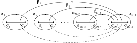
In the center-of-mass frame, the classical trajectories of the Reggeons correspond to the cycles over $N-1$ allowed bands on the Riemann surface, which we denote as $\alpha_{k}$ with $k=1$, $...$, $N-1$. By the definition, for each point $Q$ on the cycle $\alpha_{k}$ the corresponding Reggeon coordinate and momentum, $x_{j}$ and $p_{j}$, take real values. It is easy to see from Fig. 1 that the sum of all $\alpha-$cycles is homologous to zero

$$\alpha_{1}+\alpha_{2}+...+\alpha_{N-1}\approx 0$$ (4.9)

and one can choose the first $g=N-2$ $\alpha-$cycles to construct the canonical basis of cycles on $\Gamma_{N}$: $\alpha_{1}$, $...$, $\alpha_{N-2}$, $\beta_{1}$, $...$, $\beta_{N-2}$ with the intersection matrix

$$\alpha_{j}\circ\alpha_{k}=\beta_{j}\circ\beta_{k}=0\,,\qquad\alpha_{j}\circ\beta_{k}=\delta_{jk}\,.$$

The definition of the $\beta-$cycles is shown in Fig. 1. Obviously, the introduction of the $\beta-$cycles has a meaning only for $N\geq 3$ Reggeon states.

At this point we notice the important difference between $N=2$ and $N\geq 3$ Reggeon states – the appearance of the moduli for the complex curve $\Gamma_{N}$ for $g=N-2\geq 1$. To identify the moduli we observe that the curve (4.6) is invariant under transformation

$$x\to\lambda x\,,\qquad\hat{q}_{k}\to\lambda^{k}\hat{q}_{k}\,,\qquad y\to\lambda^{N}y\,,$$ (4.10)

which is induced by rescaling of the parameter $\eta$ in (3.25). Let us introduce the moduli of the hyperelliptic curve $\Gamma_{N}$ for $N\geq 3$ as

$$u_{k-2}=\hat{q}_{k}/(-\hat{q}_{2})^{k/2}=q_{k}/(-q_{2})^{k/2}\,,\qquad k=3,...,N\,,$$ (4.11)

where we used (3.25) to eliminate the dependence on arbitrary parameter $\eta$. Thus defined moduli are invariant under (4.10) and depend on the quantum numbers of the $N$ Reggeon states. It is also convenient to introduce the following variable

$$T={\left({-\hat{q}_{2}}\right)}^{1/2}=\eta{\left({-q_{2}}\right)}^{1/2}\,.$$

According to (3.16), for polynomial solutions of the Baxter equation, $u_{1},...,u_{N-2}$ and $T$ take real quantized values, such that

$$\hat{q}_{2}=-T^{2}\,,\qquad\hat{q}_{k}=T^{k}u_{k-2}\,,$$ (4.12)

with $k=3$, $...$, $N$.

The relation (4.1) defines the following meromorphic 1–differential on the hyperelliptic curve (4.6)

$$dS_{0}=dx\ln\omega(x)\cong-x\frac{d\omega}{\omega}=\frac{N\Lambda(x)-x\Lambda^{\prime}(x)}{y}dx\,.$$ (4.13)

At the vicinity of two infinities on the upper and lower sheets of the Riemann surface, $P_{\pm}$, the differential behaves as

$$dS_{0}\stackrel{{\scriptstyle x\to P_{\pm}}}{{\sim}}\mp iT\frac{dx}{x}$$

and we identify $dS_{0}$ as a dipole (unnormalized) differential of the third kind [43, 29] with the residue $\mathop{\rm res}\nolimits_{P_{\pm}}dS_{0}=\frac{1}{2\pi i}\oint_{C(P_{\pm})}dS_{0}=\pm iT$ at the first-order poles at $P_{+}$ and $P_{-}$ on the curve (4.6). Let us introduce by now standard notation for the periods of the differential $dS_{0}$

$$a_{k}=\oint_{\alpha_{k}}dS_{0}\,,\qquad a^{D}_{j}=\oint_{\beta_{j}}dS_{0}\,.$$ (4.14)

One can verify from (4.13), (4.6) and (4.4) that $a_{k}$ and $a^{D}_{k}$ take correspondingly real and pure imaginary values for the polynomial solutions. Using (4.9) one obtains that the sum of all $\alpha-$periods is given by the residue of $dS_{0}$ at infinity

$$a_{1}+a_{2}+...+a_{N-1}=-2\pi i\mathop{\rm res}\nolimits_{P_{+}}dS_{0}=2\pi T\,,$$ (4.15)

and only $N-2$ periods are linear independent. The periods are functions of $T$ and $N-2$ moduli $u_{k}$ of the curve (4.6)

$$a_{k}=a_{k}(T;u_{1},...,u_{N-2})\,,\qquad k=1,2,...,N-2$$ (4.16)

and $a^{D}_{k}$ has a similar dependence.

Substituting the explicit expression (2.11) for the transfer matrix into (4.13) we can expand the meromorphic differential $dS_{0}$ over the basis of differentials of the first and the third kind on the curve $\Gamma_{N}$, $\omega_{k}$ and $d\Omega$, respectively, as

$$dS_{0}=T\left[-2d\Omega+\sum_{k=1}^{N-2}(k+2)u_{k}d\omega_{k}\right]\,,$$

where

$$d\Omega=T\frac{dx\,x^{N-2}}{y}\,,\qquad d\omega_{k}=T^{1+k}\frac{dx\,x^{N-2-k}}{y}\,,\qquad(k=1,...,N-2)\,.$$ (4.17)

Here, additional powers of $T$ were included to ensure invariance of the differentials under transformation (4.10), which acts as $T\to\lambda T$ and leaves $u_{k}$ invariant. The differentials (4.17) depend only on the moduli $u_{k}$ but not on $T$. Taking their linear combinations one can construct the canonical basis of the holomorphic 1–differentials $d\hat{\omega}_{k}$ with $k=1$, $...$, $N-2$

$$d\hat{\omega}_{k}=\sum_{j=1}^{N-2}U_{kj}(u)d\omega_{j}\,,\qquad\oint_{\alpha_{j}}d\hat{\omega}_{k}=2\pi\delta_{jk}$$ (4.18)

and the normalized differential of the third kind, $d\hat{\Omega}$, with the residue $\mathop{\rm res}\nolimits_{P_{\pm}}d\hat{\Omega}=\pm 1$ at the first-order poles $P_{\pm}$

$$d\hat{\Omega}=2id\Omega+i\sum_{j=1}^{N-2}V_{j}(u)d\omega_{j}\,,\qquad\oint_{\alpha_{j}}d\hat{\Omega}=0\,.$$ (4.19)

Here, $U_{kj}$ and $V_{j}$ are real coefficients depending on the moduli of the curve $\Gamma_{N}$. Then, for given values of the periods (4.14) the differential $dS_{0}$ can be expanded over the canonical basis as

$$dS_{0}=iTd\hat{\Omega}+\sum_{k=1}^{N-2}\frac{a_{k}}{2\pi}d\hat{\omega}_{k}\,.$$ (4.20)

It is interesting to note that similar differential appears in the Seiberg-Witten description of the low-energy effective action of $N=2$ SUSY Yang-Mills theory [9]. The differential (4.20) defines the asymptotic solution (3.30) of the Baxter equation, which being substituted into (3.25), (3.5) and (3.13) determines the spectrum of the $N$ Reggeon compound states.

4.2. Hamiltonian flows

The phase space for the system of $N$ Reggeons is given by the direct product of the cycles $\alpha_{j}$ $(j=1,2,...,N-1)$ on the Riemann surface $\Gamma_{N}$ times the center-of-mass motion. The set of points $Q_{1}$, $...$, $Q_{N-1}$ on the Riemann surface situated one each on the $\alpha-$cycles corresponds to the real values of the canonical Reggeon coordinates $(x_{j},p_{j})$ and provides the coordinates on the level surface $\hat{q}_{k}=\mbox{const.}$ Let us consider the Hamiltonian flow of the Reggeons on the curve $\Gamma_{N}$, generated by the hamiltonians $\hat{q}_{k}$ with the canonical Poisson bracket in the separated variables $(x_{j},p_{j})$ as

$$\frac{\partial x_{j}}{\partial\tau_{k}}=\{x_{j},\hat{q}_{k}\}=\frac{\partial\hat{q}_{k}}{\partial p_{j}}\,,$$ (4.21)

with $\tau_{k}$ being the corresponding “times”. To calculate the r.h.s. we use the properties (4.2) and (4.3) of the separated variables to get

$$2(\cosh p_{j}-1)x_{j}^{N}=\hat{q}_{2}x_{j}^{N-2}+\hat{q}_{3}x_{j}^{N-3}+...+\hat{q}_{N}$$ (4.22)

with $j=1$, $...$, $N-1$ and invert these relations to find the expressions for the hamiltonians $\hat{q}_{k}$. It is convenient to introduce $(N-1)\times(N-1)$ matrix $W$ inverse to the Vandermonde matrix

$$(W^{-1})_{jk}=x_{j}^{N-k}\,,\qquad W_{kj}=\frac{(-)^{k}}{m^{\prime}(x_{j})}\frac{\partial}{\partial x_{j}}t_{k-1}(x)\,,$$ (4.23)

where $1\leq j\leq N-1$, $2\leq k\leq N$, $m(x)=\prod_{j=1}^{N-1}(x-x_{j})$ and $t_{k}=\sum_{1\leq j_{1}<...<j_{k}\leq N-1}x_{j_{1}}...x_{j_{k}}$ are symmetric polynomials. Then, one obtains from (4.22) the expressions for the hamiltonians

$$\hat{q}_{k}=2\sum_{j=1}^{N-1}W_{kj}(x)x_{j}^{N}(\cosh p_{j}-1)\,,$$ (4.24)

which have a nonpolynomial kinetical part and which are very similar to analogous Hamiltonians for the classical Toda chain of $N$ interacting particles [23, 42]. The hamiltonians (4.24) form a commutative family with respect to the Poisson bracket (4.21). Substitution of (4.24) into (4.21) yields the equations of motion for the Reggeon coordinates

$$\frac{\partial x_{j}}{\partial\tau_{k}}=2W_{kj}(x)x_{j}^{N}\sinh p_{j}=W_{kj}(x)\sqrt{\Lambda^{2}(x_{j})-4x_{j}^{2N}}\,,$$ (4.25)

where (4.5) and (4.3) were used. These relations are well-known in the theory of finite-gap solutions of the KP/Toda systems as equations for zeros (or poles) of the Baker-Akhiezer function [29].

The integration of the evolution equations (4.25) can be easily performed by the Abel map [29, 43, 30]. Indeed, multiplying the both sides of (4.25) by $x_{j}^{N-l}$ and taking into account that according to the definition (4.23), $\sum_{j}W_{kj}x_{j}^{N-l}=\delta_{jl}$, we get

$$d\tau_{k}=\sum_{j=1}^{N-1}\frac{dx_{j}\,x_{j}^{N-k}}{\sqrt{\Lambda^{2}(x_{j})-4x_{j}^{2N}}}\,,$$ (4.26)

where $k=2$, $...$, $N$. Comparing (4.26) with the definition (4.17) of the differentials $d\omega_{k}$ and $\Omega$ we obtain

$$t_{2}\equiv\tau_{2}\,T=\sum_{j=1}^{N-1}\int^{Q_{j}}d\Omega\,,\qquad t_{k}\equiv\tau_{k}\,T^{k-1}=\sum_{j=1}^{N-1}\int^{Q_{j}}d\omega_{k-2}\,,$$ (4.27)

where $k=3$, $...$, $N$ and the points $Q_{j}$ lie on the Riemann surface one each over the $\alpha-$cycles. Finally, we introduce a new set of the Reggeon coordinates

$$(Q_{1},...,Q_{N-1})\to(\vartheta,\varphi_{1},...,\varphi_{N-2})\,,$$ (4.28)

where

$$\vartheta=-i\sum_{j=1}^{N-1}\int^{Q_{j}}d\hat{\Omega}\,,\qquad\varphi_{k}=\sum_{j=1}^{N-1}\int^{Q_{j}}d\hat{\omega}_{k}$$ (4.29)

and $k=1$, $...$, $N-2$. Using the definitions (4.27), (4.18) and (4.19) we find that the equations of motion (4.26) are trivially integrated in these variables

$$\vartheta=2t_{2}+\sum_{j=1}^{N-2}V_{j}(u)t_{j+2}\,,\qquad\varphi_{k}=\sum_{j=1}^{N-2}U_{kj}(u)t_{j+2}\,,$$ (4.30)

with $U_{kj}$ and $V_{j}$ being $t-$independent functions of the moduli.

The following remarks are in order. The number of points $Q_{j}$ in (4.28) is equal to the number of allowed bands, $N-1=g+1$, and it does not match the genus of the Riemann surface $\Gamma_{N}$. The vector with the coordinates $\varphi=(\varphi_{1},...,\varphi_{N-2})$ depends on the integration path entering into (4.29) and it defines the point on the Jacobian ${\cal J}(\Gamma_{N})$ of the complex curve (4.6). At the same time, the variable $\vartheta$ is related to the differential $d\hat{\Omega}$ and it starts to play a special role. Then, in new coordinates, $\vartheta$ and $(\varphi_{1},...,\varphi_{N-2})\in{\cal J}(\Gamma_{N})$, the relations (4.30) describe a “fast” winding of the Reggeons around the Jacobi torus of the Riemann surface $\Gamma_{N}$ and a “slow” periodic motion in $\vartheta$. The corresponding periods can be evaluated using (4.29), (4.18) and (4.19) as

$$\oint_{\alpha_{j}}d\varphi_{k}=2\pi\delta_{jk}\,,\qquad\oint_{\alpha_{N-1}}d\varphi_{k}=-\sum_{j=1}^{N-2}\oint_{\alpha_{j}}\varphi_{k}=-2\pi$$

and

$$\oint_{\alpha_{j}}d\vartheta=0\,,\qquad\oint_{\alpha_{N-1}}d\vartheta=i\sum_{j=1}^{N-2}\oint_{\alpha_{j}}d\hat{\Omega}-2\pi\mathop{\rm res}\nolimits_{P_{+}}d\hat{\Omega}=-2\pi\,,$$

where $j,\,k=1$, $...$, $N-2$. We recall that the generators of “fast” motion in times $t_{3}$, $...$, $t_{N}$ are the hamiltonians $q_{3}$, $...$, $q_{N}$, while the hamiltonian $q_{2}$ generates “slow” drift of the system in time $t_{2}$.

4.3. Action-angle variables

The periods $a_{j}$ and the coordinates $\varphi_{j}$ have a simple interpretation in terms of the action-angle variables for the $N$ Reggeon state. The differential $dS_{0}$ becomes the generating function of the canonical transformation from the separated coordinates $(x_{j},p_{j})$ to the action-angle variables $(\phi_{j},J_{j})$. Namely, the action variables are defined as

$$J_{k}=\frac{1}{2\pi}\oint_{\alpha_{k}}dx\,p(x)=\frac{1}{2\pi}\oint_{\alpha_{k}}dS_{0}\equiv\frac{a_{k}}{2\pi}$$

and the corresponding angles are given by

$$\phi_{k}=\frac{\partial S}{\partial J_{k}}\,,\qquad S=\sum_{k=1}^{N-1}\int^{x_{k}}dx\,p(x)=\sum_{k=1}^{N-1}\int^{Q_{k}}dS_{0}\,,$$

where $x_{k}$ belongs to the $k-$th allowed band. Substituting the canonical form (4.20) of the differential $dS_{0}$ into this relation and taking into account that $T=\sum_{j=1}^{N-1}J_{k}$ due to (4.15), one finds

$$\phi_{k}=\varphi_{k}-\vartheta\,,\quad\phi_{N-1}=-\vartheta\,,\quad\oint_{\alpha_{j}}d\phi_{j^{\prime}}=2\pi\delta_{jj^{\prime}}\,,$$ (4.31)

where $j,j^{\prime}=1$, $...$, $N-1$ and the last identity follows from (4.18) and (4.19). The angles $\phi_{k}$ describe the winding of the Reggeons around $\alpha-$cycles on the Riemann surface $\Gamma_{N}$ and the corresponding basic oscillation frequencies are defined as

$$\phi_{k}=\Theta_{kj}\tau_{j}\,.$$

The frequencies $\Theta_{kj}$ do not depend on the times $\tau_{j}$ and they can be easily evaluated from (4.31) and (4.30) in terms of the coefficients $U$ and $V$ entering into definition of normalized differentials (4.18) and (4.19) .

Summarizing our consideration of the dynamics of the $N$ Reggeon system governed by the leading term in the asymptotic expansion of the Baxter equation solution (3.30), we found that as a result of the composition of the maps

$$(z_{j},\pi_{j})\to(x_{j},p_{j})\to(Q_{j})\in\Gamma_{N}\to\vartheta,(\varphi_{1},...,\varphi_{N-2})\in{\cal J}(\Gamma_{N})$$

the Reggeons have linear trajectories (4.30) on the Jacobian of the Riemann surface $\Gamma_{N}$. Performing inverse transformations one can construct the explicit expressions for the holomorphic Reggeon coordinates by means of the Riemann theta functions corresponding to $\Gamma_{N}$ [43, 30]. The resulting expressions are similar to the soliton solutions of the KP/Toda hierarchy [30, 29, 43] and in the center-of-mass frame of the $N$ Reggeon compound state, $P=0$, they can be represented as

$$z_{k}=z_{k}(t_{2},t_{3},...,t_{N})=\exp{\left({2it_{2}}\right)}\cdot\Psi_{k}(t_{3}U^{(1)}+...+t_{N}U^{(N-2)};u_{1},...,u_{N-2})\,.$$ (4.32)

Here, $\Psi_{k}(\varphi_{1},...,\varphi_{N-2};u_{1},...,u_{N-2})$ is a $2\pi$ periodic function of the variables $\varphi_{j}$ given by (4.30). It depends on the parameters $u_{k}$ defined in (4.11) and on the $(N-2)-$dimensional wave vectors $U^{(k)}=(U_{1k},...,U_{N-2,k})$ built from the matrix $U$. In analogy with the KP/Toda solitons [30, 43, 29], the wave vectors can be expressed in terms of the $\beta-$periods of the differentials of the second kind, $d\hat{\Omega}_{k}$, on the curve $\Gamma_{N}$, normalized as [43]

$$\oint_{\alpha_{j}}d\hat{\Omega}_{k}=0\,,\qquad d\hat{\Omega}_{k}\stackrel{{\scriptstyle\xi\to 0}}{{\sim}}\frac{d\xi}{\xi^{k+1}}\,,$$

where $\xi=T/x\to 0$ is a local parameter on the curve $\Gamma_{N}$ at the vicinity of infinity $P_{+}$ on the upper sheet. Using the well-known property [43], that the $\beta-$periods of the differentials $d\hat{\Omega}_{k}$ are related to the behaviour of the holomorphic differential $d\hat{\omega}_{k}$ near infinity $P_{+}$ as

$$\oint_{\beta_{j}}d\hat{\Omega}_{k}=\frac{1}{k!}\partial_{\xi}^{k-1}f_{j}(\xi)\left.\right|_{\xi=0}\,,\qquad d\hat{\omega}_{j}\stackrel{{\scriptstyle\xi\to 0}}{{\sim}}f_{j}(\xi)d\xi$$

and substituting (4.18) and (4.17) into this relation, one can obtain the following expressions for the coefficients $U_{kj}\equiv U^{(j)}_{k}$

$$U^{(1)}_{k}=2i\oint_{\beta_{k}}d\hat{\Omega}_{1}\,,\qquad U^{(2)}_{k}+\frac{u_{1}}{2}U^{(1)}_{k}=4i\oint_{\beta_{k}}d\hat{\Omega}_{2}\,,\ \ ...\ \ .$$ (4.33)

To understand the origin of the first factor in (4.32) involving the time $t_{2}=\tau_{2}T$, we observe that (4.32) gives an exact solution to the hierarchy of the conservation laws

$$\frac{\partial z_{k}}{\partial\tau_{j}}=\{z_{k},\hat{q}_{j}\}\,.$$

Let us consider the evolution of $z_{k}$ in time $\tau_{2}$. Replacing in (2.14) $\pi_{j}=-i\eta\partial_{z_{j}}$ by their classical analogs, one finds that the Hamiltonian $\hat{q}_{2}$ is related to the holomorphic part of the total angular momentum of the $N$ Reggeon system in the center-of-mass rest frame, $\sum_{j}\pi_{j}=P=0$, as

$$\hat{q}_{2}\equiv-T^{2}={\left({\sum_{k=1}^{N}z_{k}\pi_{k}}\right)}^{2}\,.$$

Therefore, the evolution of the Reggeon holomorphic coordinates in time $\tau_{2}$ becomes trivial

$$\partial_{\tau_{2}}z_{k}=\{z_{k},\hat{q}_{2}\}=2iTz_{k}\Longrightarrow z_{k}\sim\exp{\left({2i\tau_{2}T}\right)}$$

and it corresponds to the rotation of the $N$ Reggeon system on the 2-dimensional plane of the impact parameters (2.2) with the angular momentum $2T$. Then, using the definitions (4.12), (2.14) and (2.15) one obtains that in the large $h$ limit the total angular momentum of the soliton wave is equal by the Lorentz spin $m$ of the $N$ Reggeon state

$$2T=2\sqrt{h(h-1)}=2{\left({h-\frac{1}{2}}\right)}+{\cal O}(h^{-1})=m\,.$$

Thus, the first factor in (4.32) describes the rotation of the $N$ Reggeon system around its center-of-mass in the 2-dimensional impact parameter space. For $N=2$ Reggeon state, the BFKL Pomeron, this becomes the only mode of the Reggeon motion. For $N\geq 3$ the quasiclassical dynamics of the $N$ Reggeon compound states becomes much more interesting due to appearance of the soliton excitations (4.32). The space of the parameters $u_{1}$, $...$, $u_{N-2}$ of the $N$ Reggeon soliton waves coincides with the moduli space ${\cal M}$ of the hyperelliptic curve $\Gamma_{N}$. The coordinates on ${\cal M}$ are determined by the values of the quantum numbers $q_{2}$, $...$, $q_{N}$.

4.4. Singularities on the moduli space

The numerical solutions of the Baxter equation [21, 26] indicate that for fixed $q_{2}$ the possible values of the quantum numbers $q_{3}$, $...$, $q_{N}$ occupy a compact region in $(N-2)-$dimensional space with the boundary defined by the hypersurface (3.22). Let us show that the hypersurface (3.22) can be identified from the analysis of singularities on the moduli space ${\cal M}$ of the $N$ Reggeon soliton waves. It is well-known [43, 29] that the curve $\Gamma_{N}$ becomes singular only when two branch points merge, $\sigma_{j}=\sigma_{j+1}$ (see Fig. 1). Since the positions of $\sigma_{j}$ depend on the values of the quantum numbers, the latter relation implies certain conditions on $q_{k}$.

For $N=2$ Reggeon states, one finds the branch points of the curve (4.7) as

$$-\sigma_{1}=\sigma_{2}=\frac{T}{2}\,.$$

Since $T^{2}=-\hat{q}_{2}>0$ for the polynomial solutions, the values of $\sigma_{1}$ and $\sigma_{2}$ are always real and different. Thus, the curve $\Gamma_{2}$ does not have any singularities and this is in agreement with the fact [3, 26] that the exact solution of the Baxter equation for $N=2$ is well defined and the asymptotic expansion of the energy (3.21) is Borel summable for $N=2$.

For $N=3$ Reggeon states, or the QCD Odderon, the curve (4.8) has four branching points

$$4\sigma_{j}^{3}+\hat{q}_{2}\sigma_{j}+\hat{q}_{3}=0\,,\quad(j=1,2,3)\,,\qquad\sigma_{4}=-\frac{\hat{q}_{3}}{\hat{q}_{2}}\,.$$

To classify all possible solutions we introduce the “effective” discriminant $\Delta$ of the curve $\Gamma_{3}$ as

$$\Delta=16\sigma^{2}_{4}(\sigma_{1}-\sigma_{2})^{2}(\sigma_{2}-\sigma_{3})^{2}(\sigma_{3}-\sigma_{1})^{2}=\hat{q}_{2}^{4}\ u_{1}^{2}(1-27u_{1}^{2})\,,$$

where $u_{1}$ was defined in (4.11). Then, for $\Delta>0$ all roots $\sigma_{k}$ are real; for $\Delta<0$ two roots are real and two remaining roots are complex conjugated to each other and, finally, for $\Delta=0$ two roots coincide and the curve $\Gamma_{3}$ becomes singular.

Therefore, in order to be able to construct two real intervals corresponding to the classical motion of the Reggeons in the separated coordinates $x_{1}$ and $x_{2}$ one has to require $\Delta>0$. If one assumes that the moduli space ${\cal M}$ is the complex $u_{1}-$plane, then the singularities are located at three points

$$u_{1}^{\rm crit}=-\frac{1}{\sqrt{27}}\,,\ 0\ \ {\rm and}\ \ \frac{1}{\sqrt{27}}$$ (4.34)

and the polynomial solutions of the Baxter equation for $N=3$ Reggeon states correspond to the real values of $u_{1}$ shown in Fig. 2 such that

$$0<u_{1}^{2}<\frac{1}{27}\,.$$ (4.35)

For $\lambda=-1$ the property (4.10) of the curve $\Gamma_{3}$ leads to the symmetry on the moduli space ${\cal M}$ under $u_{1}\leftrightarrow-u_{1}$.

Figure 2: The possible values of $u_{1}$ for $N=3$ Reggeon states corresponding to the polynomial solutions of the Baxter equation. The dots indicate the positions of singularities.

The relations (4.34) and (4.35) are in complete agreement with the numerical results [21, 26] and with asymptotic expansions of the solutions of the Baxter equation, (3.23). A similar analysis can be carried out for higher $N>3$ Reggeon states [26].

Any point on the moduli space ${\cal M}$ corresponds to a certain Riemann surface $\Gamma_{N}$ and it describes the compound state of $N$ Reggeons with the quantum numbers defined by (4.12). The energy $\varepsilon_{N}$ of these states becomes the function on the moduli space and it is naturally to expect that singularities on the moduli space ${\cal M}$ control the analytical properties of the functions $\varepsilon_{N}$ for $N\geq 3$. They are responsible for the appearance of Borel singularities in the asymptotic expansion of the energy (3.21) for $N\geq 3$.

5. Quantization conditions

Let us discuss the quantization conditions for eigenvalues of the integrals of motion $q_{2}$, $...$, $q_{N}$. The quantization of $q_{2}$ follows from the definition (2.14) after one takes into account that possible values of the conformal weight are given by (2.15). The polynomial solutions of the Baxter equation correspond to the special values (3.14) of quantized $q_{2}=-h(h-1)$. In this case one has to establish the quantization conditions for the remaining charges $q_{3}$, $...$, $q_{N}$ and then try to generalize them from integer conformal weight $h$ to all possible complex values (2.15).

Inverting the dependence (4.16) and using (4.15) one can obtain that the quantized values of the moduli (4.11), or equivalently $q_{3}$, $...$, $q_{N}$, are determined by $q_{2}$ and by $N-2$ linear independent periods $a_{k}$ of the differential $dS_{0}$ defined in (4.14)

$$u_{k}=u_{k}(\hat{q}_{2};a_{1},a_{2},...,a_{N-2})\,,\qquad k=1,...,N-2\,.$$ (5.1)

Although $\hat{q}_{2}$ and $a_{k}$ depend separately on the parameter $\eta$, this dependence is cancelled inside the function $u_{k}$ due to invariance of the moduli under transformation (4.10).

The periods $a_{k}$ have a simple interpretation in terms of the roots $\lambda_{j}$ of the solutions (3.15) of the Baxter equation. We recall that the solutions $Q(x)$ define the wave function of the $N$ Reggeon state in the separated coordinates (3.5). Therefore, the roots $\lambda_{j}$ of $Q(x)$ being the zeros of the Reggeon wave function should belong to the intervals of the classical motion of Reggeons, that is to the $N-1$ allowed bands on the Riemann surface $\Gamma_{N}$. Let us denote by $n_{k}$ the number of roots of $Q(x)$ (including the $N-$time degenerate root at $x=0$) which belong to the $k-$th allowed band, $\lambda_{j}\in[\sigma_{2k-1},\sigma_{2k}]$,

$$n_{k}\geq 0\,,\qquad\sum_{k=1}^{N-1}n_{k}=h$$ (5.2)

and $n_{j}\geq N$ if the root $x=0$ belongs the $j-$interval $\sigma_{2j-1}<0<\sigma_{2j}$. Then, it follows from (3.28) that the meromorphic differential $dS$ has first-order poles on the Riemann surface $\Gamma_{N}$ at $x=\lambda_{j}$ and its periods around $\alpha-$cycles count the number of roots

$$\oint_{\alpha_{k}}dS=2\pi\eta n_{k}\,.$$

Substituting the expansion (3.27) of $dS$ in powers of $\eta$ one gets

$$a_{k}\equiv\oint_{\alpha_{k}}dS_{0}=2\pi\eta{\left({n_{k}+\frac{1}{2}}\right)}+{\cal O}(\eta^{2})\,,$$ (5.3)

where ${\cal O}(\eta^{2})$ term takes into account the contribution of higher terms in the expansion (3.27). The relations (5.3) take the form of Bohr-Sommerfeld quantization conditions for the Reggeon wave function (3.30).

Substituting (5.3) into (5.1) we find that the moduli of the Riemann surface, or equivalently the integrals of motion $q_{3}$, $...$, $q_{N}$, become quantized and, in accordance with our expectations (3.17), their values are parameterized by $q_{2}$ and by the set of positive integer numbers $n_{k}$. However, trying to find the dependence of moduli on $n_{k}$ from (5.1) and (5.3), one has to take into account that the periods $a_{k}$ themselves are functions of the moduli due to ${\cal O}(\eta^{2})$ term in (5.3), which does not depend on integers $n_{k}$ and has the general form $\eta^{2}{\left({-\hat{q}_{2}}\right)}^{1/2}H(\{u_{k}\})$. Here, $H$ is a complicated function of the moduli and $\hat{q}_{2}$ is needed to restore the scaling dimension of $a_{k}$ in $\eta$ under transformation (4.10). Then, using independence of $u_{k}$ on $\eta$ one can put $\eta={\left({-q_{2}}\right)}^{-1/2}$ in (5.1) and represent the general solution of (5.1) and (5.3) as

$$u_{k}=\bar{u}_{k}{\left({\delta_{1},\delta_{2},...,\delta_{N-2};q_{2}^{-1}}\right)}\,,\qquad\delta_{j}\equiv\frac{n_{j}+\frac{1}{2}}{{\left({-q_{2}}\right)}^{1/2}}\,.$$ (5.4)

One possibility to define the function $\bar{u}_{k}$ is to find its asymptotic expansion in inverse powers of the conformal weight using the series (3.21),

$$u_{k}=\sum_{k\geq 0}c_{k}(n)\,h^{-k}$$ (5.5)

with $q_{2}=-h(h-1)$ and $n_{j}=\mbox{fixed}$. However, due to the presence of singularities on the moduli space ${\cal M}$, the series (5.5) turns out to be non Borel summable. Let us now change the parameters of the expansion and expand the function (5.4) in powers of $q_{2}^{-1}$ keeping $\delta_{j}=\mbox{fixed}$. As example, one uses the result [26] for the large $h$ expansion of $u_{1}$ to ${\cal O}(h^{-8})$ order for $N=3$ Reggeon states to convert it into the following form

$$u_{1}=\sum_{k=0}^{\infty}u_{1}^{(k)}(\delta)\,q_{2}^{-k}\,,$$ (5.6)

where the leading term is given by

$$u_{1}^{(0)}(\delta)=\frac{1}{\sqrt{27}}\left(1-3\,\delta+2\,{\delta}^{2}-{\frac{2}{9}}{\delta}^{3}+{\frac{10}{81}}{\delta}^{4}+{\frac{38}{243}}{\delta}^{5}+{\frac{448}{2187}}{\delta}^{6}+{\frac{1840}{6561}}{\delta}^{7}+{\cal O}(\delta^{8})\right)\,.$$ (5.7)

We notice that the expansion (5.6) goes over integer powers of $1/q_{2}={\cal O}(h^{-2})$, while the original series (5.5) had a much bigger parameter of the expansion, $1/h$.

Let us consider now the asymptotic approximation to solution of the Baxter equation given by the expression (3.30), in which we neglect all nonleading ${\cal O}(\eta)$ corrections to the exponent. In this limit, there are no ${\cal O}(\eta^{2})$ corrections to the periods $a_{k}$ in (5.3) and the expressions (5.1) and (5.4) for quantized moduli look like

$$u_{k}^{(0)}=u_{k}(\hat{q}_{2};a_{1},a_{2},...,a_{N-2})\big{|}_{a_{k}=2\pi\eta{\left({n_{k}+\frac{1}{2}}\right)}}=\bar{u}_{k}(\delta_{1},\delta_{2},...,\delta_{N-2};0)\,,$$ (5.8)

where the parameters $\delta_{k}$ were defined in (5.4).

To obtain all possible values of quantum numbers $q_{3}$, $...$, $q_{N}$ one has to evaluate the moduli (5.8) for different sets of integers $n_{1}$, $...$, $n_{N-2}$ and substitute them into (4.12). Let us consider (5.8) as a definition of a continuous function of real positive $q_{2}$, which for $q_{2}=-h(h-1)$ and $h$ positive integer gives quantized $q_{k}$. Then, for different possible sets (5.2) of integers $n_{k}$ the functions (5.8) define the family of curves on the moduli space ${\cal M}$. Each curve describes the flow on the moduli space ${\cal M}$ in the “slow” time $q_{2}$ and it has a distinguished property that the values of the periods $a_{k}$ are preserved. As example [26], the flow of quantized $q_{3}$ as a function of $q_{2}$ for $N=3$ Reggeon states and fixed value of integer $n_{1}=4$ is shown by solid line in Fig. 3. This curve induces the flow on the moduli space indicated by the solid line in Fig. 2.

Figure 3: One of the curves describing the flow of quantized $q_{3}$ for $N=3$ Reggeon states. The circles represent the results of numerical calculations. Three dashed lines correspond to the singularities on the moduli space (4.34).

For $N=3$ Reggeon states, $u_{1}^{(0)}$ is equal to the leading term of the expansion (5.6) given by (5.7). Comparing (5.7) with (4.34) we find that the expression (5.7) provides a weak coupling expansion of the moduli in $\delta$ around one of the singularities on the moduli space in Fig. 2. To approach two remaining singular points one has to develop the strong coupling expansion of the moduli.

The Seiberg-Witten formalism [2] gives us a powerful method of calculating the moduli (5.8), based on the Whitham equations and on the remarkable property of duality between strong and weak coupling expansions of the moduli $u_{k}$ in parameters $\delta_{j}$ [44]. In application to the $N=3$ Reggeon states, the duality originates from the property [2] that the quantity $(a_{1}(u_{1}),a^{D}_{1}(u_{1}))$, built from the periods (4.14) of the differential $dS_{0}$ on the curve $\Gamma_{3}$, has well-known monodromies around the singular points (4.34). The monodromies are given by $2\times 2$ matrices, which belong to the subgroup $\Gamma(2)$ of the $SL(2,\mathchoice{\hbox{\cmss Z\kern-3.99994ptZ}}{\hbox{\cmss Z\kern-3.99994ptZ}}{\lower 0.9pt\hbox{\cmsss Z\kern-4.39993ptZ}}{\lower 1.2pt\hbox{\cmsss Z\kern-4.39993ptZ}})$ group consisting of the matrices congruent to 1 modulo 2. The symmetry of the spectral curve $\Gamma_{3}$ under $u_{1}\to-u_{1}$ leads to the following property of the moduli (5.7) [44]

$$u_{1}(1-\delta)=-u_{1}(\delta)\,,$$

which together with (5.7) allows us to identify the values of $\delta$ corresponding to the singularities (4.34) on the moduli space as

$$\delta^{\rm crit}=1\,,\ \frac{1}{2}\ \ {\rm and}\ \ 0\,,$$

respectively. Having expressions for the monodromy of $(a_{1}(u_{1}),a^{D}_{1}(u_{1}))$ one can determine the asymptotic behaviour of the moduli around these points in the following form [44]

$$\delta-1\sim-\sqrt{3}{\left({u_{1}+\frac{1}{\sqrt{27}}}\right)}\,,\qquad\delta-\frac{1}{2}\sim\frac{3}{\pi}u_{1}{\left({\ln u_{1}-1}\right)}\,,\qquad\delta\sim-\sqrt{3}{\left({u_{1}-\frac{1}{\sqrt{27}}}\right)}\,.$$ (5.9)

These relations describe the flow of the quantum numbers shown in Fig. 3 and they can be also derived from the Whitham equations.

5.1. Whitham equations

Let us show that the flow of the moduli (5.8) in the “slow” time – variable $q_{2}$ is governed by the Whitham equations [11, 9]. We recall that the function (5.1) is inverse to (4.16) and the dependence of $u_{k}$ on $q_{2}$ in (5.8) can be found from the condition that the periods $a_{k}$ should be invariant under variations of $q_{2}$. Using the definition of the periods (4.14), this condition can be expressed as follows

$$\delta a_{k}=\delta T\oint_{\alpha_{k}}\partial_{T}dS_{0}+\delta u_{j}\oint_{\alpha_{k}}\partial_{u_{j}}dS_{0}=0\,.$$ (5.10)

To calculate the external derivatives one considers the variation of the differential $dS_{0}$ with respect to Reggeon quantum numbers. As follows from the definitions (4.13) and (4.5)

$$\delta dS_{0}=dx\frac{\delta\omega}{\omega}=\delta\Lambda(x)\frac{dx}{y}={\left({\delta q_{2}x^{N-2}+\delta q_{3}x^{N-3}+...+\delta q_{N}}\right)}\frac{dx}{y}\,,$$

where we put $\eta=1$ for simplicity. Finally, one gets

$$\frac{\partial dS_{0}}{\partial u_{j}}=Td\omega_{j}\,,\qquad\frac{\partial dS_{0}}{\partial T}=T^{-1}dS_{0}\,.$$

where holomorphic differentials $d\omega_{k}$ were defined in (4.17). Here, the first relation states that the variation of the differential $dS_{0}$ with respect to moduli is proportional to the holomorphic differential defined on the curve $\Gamma_{N}$. Being applied to (5.10), this remarkable property of the differential $dS_{0}$ leads to the Whitham equations for the moduli

$$\sum_{j=1}^{N-2}\frac{\partial u_{j}}{\partial T}T^{2}\oint_{\alpha_{k}}d\omega_{j}+\oint_{\alpha_{k}}dS_{0}=0\,.$$ (5.11)

Calculating the $\alpha-$periods of the differential $d\omega_{k}$ from (4.18) as $\oint_{\alpha_{k}}d\omega_{j}=2\pi(U^{-1})_{jk}$ and taking into account (5.3), we obtain the following system of equations

$$T^{2}\frac{\partial u_{j}}{\partial T}=-\sum_{k=1}^{N-2}{\left({n_{k}+\frac{1}{2}}\right)}U_{kj}(u)\,,$$ (5.12)

where $j=1$, $...$, $N-2$ and $U_{kj}$ are functions of the moduli $u_{1}$, $...$, $u_{N-2}$. The matrix elements of $U_{kj}$ define the wave vectors of the soliton waves (4.32) and one can rewrite (5.12) as

$$T^{2}\frac{\partial u_{j}}{\partial T}=-(v,U^{(j)})\,,$$

where notation was introduced for the vector $v_{k}=n_{k}+\frac{1}{2}$ and $(v,U^{(j)})\equiv v_{k}U_{kj}$.

For $N=3$ Reggeon states, the system (5.12) is reduced to an ordinary differential equation for the moduli $u_{1}=u_{1}(\delta)$ with $\delta=(n+\frac{1}{2})/T$

$$\frac{du_{1}}{d\delta}=U(u_{1})\,,$$ (5.13)

where $U=U^{(1)}$ was defined in (4.33). It allows us to determine exactly the function $u_{1}^{(0)}$ entering into (5.7) and study its properties at the vicinity of singularities (3.22) on the moduli space ${\cal M}$. One can show [44] that the Whitham equation (5.13) is in agreement with the weak coupling expansion (5.7) and with the asymptotics (5.9).

5.2. Boundary conditions

To solve the differential equations (5.12) and (5.13) one has to supplement them by an appropriate boundary conditions on $u_{k}$. These conditions are provided by the asymptotic behaviour of $u_{k}$ as $q_{2}\to-\infty$, which follows from the large $h$ expansion of quantum numbers (3.21).

Let us start with $N=3$ Reggeon states and examine the flow of quantized $q_{3}$ shown by solid line in Fig. 3. For $-q_{2}=h(h-1)\to\infty$ the quantized $q_{3}$ behave as $q_{3}\sim(-q_{2})^{3/2}/\sqrt{27}$ leading to the asymptotic expression for the moduli $u_{1}=\frac{1}{\sqrt{27}}$, which we identify as one of the singularities on the moduli space ${\cal M}$. Thus, the singularity on the moduli space,

$$u_{1}(\delta)=\frac{1}{\sqrt{27}}\,,\qquad\mbox{for}\quad\delta=0$$ (5.14)

becomes the starting point for the Whitham evolution (5.13). As $-q_{2}$ decreases toward the origin, $u_{1}$ passes the second singularity (3.22) at $u_{1}=0$, and for smallest $-q_{2}$, corresponding to the boundary of the polynomial solutions, $u_{1}$ approaches the third singularity on the moduli space at $u_{1}=-\frac{1}{\sqrt{27}}$. We conclude that for polynomial solutions of the $N=3$ Baxter equation, the Whitham equation (5.13) describe the trajectory on the moduli space (see Fig. 2), which goes along the real axis from $\frac{1}{\sqrt{27}}$ to $-\frac{1}{\sqrt{27}}$. The Whitham evolution of the moduli corresponding to higher $N>3$ Reggeon states follows a similar pattern. For $-q_{2}\to\infty$ the quantum numbers $q_{k}$ approach the values belonging to the critical hypersurface (3.22). The same values coincide with the positions of singularities on the moduli space ${\cal M}$, $u_{k}\sim u_{k}^{\rm sing}$ as $-q_{2}\to\infty$. Since the possible values of the moduli corresponding to the polynomial solutions occupy a compact region on the moduli space with the boundary being the singularities, the flow of $u_{k}$ will start at one singular point as $-q_{2}\to\infty$ and will finish at another singular point on ${\cal M}$ for $-q_{2}$ taking the smallest value allowed for the polynomial solutions of the Baxter equation.

As was shown in Sect. 4.2, the “time” variable in the Whitham evolution, T, is related to the total angular momentum associated with the rotation of the $N$ Reggeon system around its center-of-mass in the impact parameter space. The Whitham equations (5.12) and (5.13) describe the adiabatic perturbation of the moduli of the curve $\Gamma_{N}$ which enter as parameters into the soliton solutions (4.32) for the $N$ Reggeon states. Thus, in the leading nonlinear WKB approximation, (3.30), the $N$ Reggeon states corresponding to the integer positive conformal weight $h$ can be considered as modulated soliton waves.

We recall that till now we worked on the subspace of the polynomial solutions of the Baxter equation. The Whitham equations (5.12) and (5.13) offer a natural way of analytical continuation of the obtained expressions beyond this subclass. Let us consider for simplicity the $N=3$ Reggeon states. The evolution of $q_{3}$ is described by a smooth function of $q_{2}=-h(h-1)$ (see Fig. 3), which for $h$ in (3.14) gives the values of quantized $q_{3}$. We observe that, first, the same function allows us to define formally $q_{3}$ corresponding to half-integer $h$ in (2.15) and, second, the evolution of $q_{3}$ inevitably leads to the region of small and positive $q_{2}$, where polynomial solutions do not exist. Applying the Whitham equations (5.12) and (5.13) in these two cases one assumes that the above interpretation of the $N$ Reggeon states as modulated soliton waves holds for any integer and half-integer conformal weight $h$. One may also try to apply the Whitham equations for an arbitrary complex quantized conformal weights (2.15), but the important difference with real $h$ is that one has to find now the initial conditions similar to (5.14).

6. Conclusions

The Regge asymptotics of hadronic scattering amplitudes in high-energy QCD are controlled by the color-singlet compound states of Reggeons. Reggeons appear as a new collective degrees of freedom of QCD in the Regge limit and their dynamics in four dimensions is described by the effective (1+1)-dimensional Hamiltonian, which exhibits remarkable properties of integrability. The system of $N$ interacting Reggeons in the multi-color limit resembles very much the 1-dimensional Heisenberg spin $s=0$ chain with $N$ sites. It has enough number of conserved charges $q_{k}$ to be completely integrable. To diagonalize the $N$ Reggeon hamiltonian and calculate the spectrum of the Reggeon compound states, QCD Pomerons and Odderons, we defined a new set of Reggeon coordinates, in which $N$ coupled Schrödinger equations for eigenvalues of the conserved charges $q_{k}$ become separated and are replaced by the Baxter equation (3.12). The solutions of the Baxter equation, depending on the set of quantum numbers $q_{k}$, define the energy and the wave function of the $N$ Reggeon state in the separated variables. It is the Baxter equation that summarizes the QCD dynamics of Reggeons in the separated coordinates and whose nonlinear WKB expansion gives rise to the integrable structures well-known from the finite-gap solutions of the soliton equations and their Whitham deformations.

The leading term of the nonlinear WKB expansion of the polynomial solutions of the Baxter equation defines the hyperelliptic Riemann surface $\Gamma_{N}$ as the level surface of the integrals of motion $q_{k}=\mbox{const.}$ and the meromorphic 1-differential $dS_{0}$ on it. The conserved charges $q_{k}$ generate the Hamiltonian flows of Reggeons on $\Gamma_{N}$ and the exact solution of the arising hierarchy of the evolution equations is given by the Reggeon soliton wave. The moduli $u_{k}$ of $\Gamma_{N}$ for $N\geq 3$ depend on the quantum numbers of the Reggeon states and enter as parameters into the soliton solutions. The possible values of $q_{3}$, $...$, $q_{N}$ are quantized and they determine the family of curves on the moduli space ${\cal M}$. Each curve describes the flow on ${\cal M}$, which is governed by the Whitham equations. These equations describe the adiabatic perturbation of the Reggeon soliton waves and the properties of their solutions will be considered in the forthcoming paper [44].

We would like to mention in conclusion that had we perform a similar nonlinear WKB analysis of the Baxter equation for Toda chain (3.24) in the special case $\hbar=1$, we could reproduce the main ingredients of the Seiberg-Witten solution [2] of the effective action of $N=2$ supersymmetric QCD. It remains unclear, however, what are a new collective variables in $N=2$ SUSY QCD, which play a role similar to the separated coordinates of Reggeons in high-energy QCD.

References

-
[1]
G. Veneziano, Phys. Rep. 9 (1974) 199;
A.M. Polyakov, Gauge fields and strings, Chur, Harwood, 1987. - [2] N. Seiberg and E. Witten, Nucl. Phys. B426 (1994) 19; B431 (1994) 484.
- [3] L.D. Faddeev and G.P. Korchemsky, preprint ITP–SB–94–14, Apr. 1994 [hep-ph/9404173]; Phys. Lett. B 342 (1995) 311.
- [4] L.N. Lipatov, JETP Lett. 59 (1994) 596.
[5]
A. Klemm, W. Lerche, S. Yankielowicz and S. Thiesen,
Phys. Lett. B344 (1995) 169;
P.C. Argyres and A. Faraggi, Phys. Rev. Lett. 74 (1995) 3931;
U.H. Danielsson and B. Sundborg, Phys. Lett. B358 (1995) 273;
A. Brandhuber and K. Landsteiner, Phys. Lett. B358 (1995) 73;
A. Hanany and Y. Oz, Nucl. Phys. B452 (1995) 283. - [6] A. Gorsky, I. Krichever, A. Marshakov, A. Mironov and A. Morozov, Phys. Lett. B355 (1995) 466.
[7]
E. Martinec and N. Warner, Nucl. Phys. B459 (1996) 97;
T. Nakatsu and K. Takasaki, Mod. Phys. Lett. A11 (1996) 157;
T. Eguchi and S. Yang, preprint UT-728 [hep-th/9510183]. -
[8]
R. Donagi and E. Witten, Nucl. Phys. B460 (1996) 299;
E. Martinec, Phys. Lett. B367 (1996) 91;
A. Gorsky and A. Marshakov, preprint FIAN-TD-19-95, Oct 1995 [hep-th/9510224];
E. Martinec and N. Warner, preprint EFI-95-70, Nov. 1995 [hep-th/9511052]. - [9] H. Itoyama and A. Morozov, preprints ITEP-M5/95, Nov. 1995 [hep-th/9511126] and ITEP-M6/95, Dec. 1996 [hep-th/9512161].
- [10] A. Gorsky, A. Marshakov, A. Mironov and A. Morozov, Phys. Lett. B380 (1996) 75; preprint ITEP/TH-9/96, Apr. 1996 [hep-th/9604078].
[11]
G.B. Whitham, Linear and Nonlinear Waves,
John Wiley, New York, 1974;
H. Flaschka, M.G. Forest and D.W. McLaughlin, Comm. Pure Appl. Math. 33 (1980) 739;
S.Yu. Dobrokhotov and V.P. Maslov, J. Sov. Math. 16 (1981) 1433;
B.A. Dubrovin and S.P. Novikov, Russ. Math. Surv. 44 (1989) 35.
I.M. Krichever, Comm. Math. Phys. 143 (1992) 415; Comm. Pure Appl. Math. 47 (1994) 437;
B.A. Dubrovin, Comm. Math. Phys. 145 (1992) 195. - [12] K. Takasaki and T. Nakatsu, preprint KUCP–0092, Mar. 1996 [hep-th/9603069].
- [13] A. Gorsky, preprint ITEP/TH-14/96 [hep-th/9605135].
[14]
S.C. Frautschi, Regge poles and S-matrix theory,
New York, W.A. Benjamin, 1963;
V. de Alfaro and T. Regge, Potential scattering, Amsterdam, North-Holland, 1965;
P.D.B. Collins, An introduction to Regge theory and high energy physics, Cambridge University Press, 1977. - [15] H. Cheng and T.T. Wu, Expanding Protons: Scattering at High Energies, MIT Press, Cambridge, Massachusetts, 1987.
- [16] V.N. Gribov, Sov. Phys. JETP 26 (1968) 414; Nucl. Phys. B106 (1976) 189.
- [17] R. Kirschner, L.N. Lipatov and L. Szymanowski, Nucl. Phys. B425 (1994) 579.
- [18] E. Verlinde and H. Verlinde, preprint PUPT–1319, Sept. 1993 [hep-th/9302104].
[19]
J. Bartels, Nucl. Phys. B175 (1980) 365;
J. Kwiecinski and M. Praszalowicz, Phys. Lett. B94 (180) 413. -
[20]
L.A. Takhtajan and L.D. Faddeev, Russ. Math. Survey 34 (1979) 11;
E.K. Sklyanin, L.A. Takhtajan and L.D. Faddeev, Theor. Math. Phys. 40 (1980) 688;
V.E. Korepin, N.M. Bogoliubov and A.G. Izergin, Quantum inverse scattering method and correlation functions, Cambridge Univ. Press, 1993. - [21] G.P. Korchemsky, Nucl. Phys. B443 (1995) 255.
- [22] H. Flaschka and D. McLaughlin, Progr. Theor. Phys. 55 (1976) 438.
- [23] M. Gutzwiller, Ann. Phys. 133 (1981) 304.
- [24] E.K. Sklyanin, The quantum Toda chain, Lecture Notes in Physics, vol. 226, Springer, 1985, pp.196–233; Functional Bethe ansatz, in “Integrable and superintegrable systems”, ed. B.A. Kupershmidt, World Scientific, 1990, pp.8–33; Progr. Theor. Phys. Suppl. 118 (1995) 35 [solv-int/9504001].
- [25] Z. Maassarani and S. Wallon, J. Phys. A: Math. Gen. 28 (1995) 6423.
- [26] G.P. Korchemsky, Nucl. Phys. B462 (1996) 333.
- [27] R. Janik, Phys. Lett. B371 (1996) 293; Acta Phys. Polon. B27 (1996) 1275.
- [28] R. Janik and J. Wosiek, presentation pa02-059 at the ICHEP–96, Warsaw, 25–31 July 1996.
[29]
S.P. Novikov, S.V. Manakov, L.P. Pitaevskii and V.E. Zakharov,
Theory of Solitons: The Inverse Scattering Method,
Consultants Bureau, New York, 1984;
B. Dubrovin, I. Krichever and S. Novikov, Integrable systems - I, Sovremennye problemy matematiki (VINITI), Dynamical systems - 4 (1985) 179;
B.A. Dubrovin, V.B. Matveev and S.P. Novikov, Russ. Math. Surv. 31 (1976) 59. - [30] I.M. Krichever, Russ. Math. Surv. 32 (1977) 185; Func. Anal. Appl. 14 (1980) 531; 11(1977) 12.
[31]
E.A. Kuraev, L.N. Lipatov and V.S. Fadin,
Phys. Lett. B60 (1975) 50;
Sov. Phys. JETP 44 (1976) 443; 45 (1977) 199;
Ya.Ya. Balitsky and L.N. Lipatov, Sov. J. Nucl. Phys. 28 (1978) 822. - [32] L.N. Lipatov, Phys. Lett. B251 (1990) 284; B309 (1993) 394.
- [33] L.N. Lipatov, Pomeron in quantum chromodynamic, in “Perturbative QCD”, pp.411–489, ed. A.H. Mueller, World Scientific, Singapore, 1989.
- [34] V.O. Tarasov, L.A. Takhtajan and L.D. Faddeev, Theor. Math. Phys. 57 (1983) 163.
- [35] P.P. Kulish, N.Yu. Reshetikhin and E.K. Sklyanin, Lett. Math. Phys. 5 (1981) 393.
[36]
M. Henon, Phys. Rev. B9 (1974) 1921;
H. Flaschka, Phys. Rev. B9 (1974) 1924; Progr. Theor. Phys. 52 (1974) 703;
S.V. Manakov, Sov. Phys. JETP 40 (1974) 269. - [37] R.J. Baxter, Exactly Solved Models in Statistical Mechanics, Academic Press, London, 1982; Stud. Appl. Math. 50 (1971) 51.
[38]
V. Spiridonov, L. Vinet and A. Zhedanov, Lett. Math. Phys. 29
(1993) 63;
V. Spiridonov and A. Zhedanov, J. Phys. A: Math. Gen. 28 (1995) L589. - [39] V. Pasquier and M. Gaudin, J. Phys. A: Math. Gen. 25 (1992) 5243.
[40]
S.P. Novikov, Func. Anal. Appl. 24 (1990) 296;
I.M. Krichever, ETH preprint, Zürich, June 1990;
G. Moore, Comm. Math. Phys. 133 (1990) 261;
F. Fucito, A. Gamba, M. Martinelli and O. Ragnisco, Int. J. Mod. Phys. B6 (1992) 2123. -
[41]
P. Gauron and B. Nicolescu, Phys. Lett. B260 (1991) 40;
P. Gauron, L. Lukaszuk and B. Nicolescu, Phys. Lett. B294 (1992) 298;
B. Nicolescu, Nucl. Phys. (Proc.Suppl.) 25B (1992) 142. - [42] P. van Moerbeke, Invent. Math. 37 (1976) 45.
- [43] B.A. Dubrovin, Russ. Math. Surv. 36 (1981) 11.
- [44] G.P. Korchemsky, in preparation.