Feynman diagrams with the effective action

Abstract

A derivation is given of the Feynman rules to be used in the perturbative computation of the Green’s functions of a generic quantum many-body theory when the action which is being perturbed is not necessarily quadratic. Some applications are discussed.

I Introduction

The Feynman diagrammatic technique has proven quite useful in order to perform and organize the perturbative solution of quantum many-body theories. The main idea is the computation of the Green’s or correlation functions by splitting the action $S$ into a quadratic or free part $S_{Q}$ plus a remainder or interacting part $S_{I}$ which is then treated as a perturbation. From the beginning this technique has been extended to derive exact relations, such as the Schwinger-Dyson [1, 2, 3] equations, or to make resummation of diagrams as that implied in the effective action approach [4, 5] and its generalizations [6].

Consider now a generalization of the above problem, namely, to solve (i.e., to find the Green’s functions of) a theory with action given by $S+\delta S$ perturbatively in $\delta S$ but where the “unperturbed” action $S$ (assumed to be solved) is not necessarily quadratic in the fields. The usual answer to this problem is to write the action as a quadratic part $S_{Q}$ plus a perturbation $S_{I}+\delta S$ and then to apply the standard Feynman diagrammatic technique. This approach is, of course, correct but it does not exploit the fact that the unperturbed theory $S$ is solved, i.e., its Green’s functions are known. For instance, the computation of each given order in $\delta S$ requires an infinite number of diagrams to all orders in $S_{I}$. We will refer to this as the standard expansion. In this paper it is shown how to systematically obtain the Green’s functions of the full theory, $S+\delta S$, in terms of those of the unperturbed one, $S$, plus the vertices provided by the perturbation, $\delta S$. Unlike the standard expansion, in powers of $S_{I}+\delta S$, the expansion considered here is a strict perturbation in $\delta S$ and constitutes the natural extension of the Feynman diagrammatic technique to unperturbed actions which are not necessarily quadratic. We shall comment below on the applications of such an approach.

II Many-body theory background

A Feynman diagrams and standard Feynman rules

In order to state our general result let us recall some well known ingredients of quantum many-body theory (see e.g. [5]), and in passing, introduce some notation and give some needed definitions. Consider an arbitrary quantum many-body system described by variables or fields $\phi^{i}$, that for simplicity in the presentation will be taken as bosonic. As will be clear below, everything can be generalized to include fermions. Without loss of generality we can use a single discrete index $i$ to represent all the needed labels (DeWitt notation). For example, for a relativistic quantum field theory, $i$ would contain space-time, Lorentz and Dirac indices, flavor, kind of particle and so on. Within a functional integral formulation of the many-body problem, the expectation values of observables, such as $A[\phi]$, take the following form:

$$\langle A[\phi]\rangle=\frac{\int\exp\left(S[\phi]\right)A[\phi]\,d\phi}{\int\exp\left(S[\phi]\right)\,d\phi}\,.$$ (1)

Here the function $S[\phi]$ will be called the action of the system and is a functional in general. Note that in some cases $\langle A[\phi]\rangle$ represents the time ordered vacuum expectation values, in other the canonical ensemble averages, etc, and also the quantity $S[\phi]$ may correspond to different objects in each particular application. In any case, all (bosonic) quantum many-body systems can be brought to this form and only eq. (1) is needed to apply the Feynman diagrammatic technique. As already noted, this technique corresponds to write the action in the form $S[\phi]=S_{Q}[\phi]+S_{I}[\phi]$:

$$S_{Q}[\phi]=\frac{1}{2}m_{ij}\phi^{i}\phi^{j}\,,\qquad S_{I}[\phi]=\sum_{n\geq 0}\frac{1}{n!}g_{i_{1}\dots i_{n}}\phi^{i_{1}}\cdots\phi^{i_{n}}\,,$$ (2)

where we have assumed that the action is an analytical function of the fields at $\phi^{i}=0$. Also, a repeated indices convention will be used throughout. The quantities $g_{i_{1}\dots i_{n}}$ are the coupling constants. The matrix $m_{ij}$ is non singular and otherwise arbitrary, whereas the combination $m_{ij}+g_{ij}$ is completely determined by the action. The free propagator, $s^{ij}$, is defined as the inverse matrix of $-m_{ij}$. The signs in the definitions of $S[\phi]$ and $s^{ij}$ have been chosen so that there are no minus signs in the Feynman rules below. The $n$-point Green’s function is defined as

$$G^{i_{1}\cdots i_{n}}=\langle\phi^{i_{1}}\cdots\phi^{i_{n}}\rangle\,,\quad n\geq 0\,.$$ (3)

Let us note that under a non singular linear transformation of the fields, and choosing the action to be a scalar, the coupling constants transform as completely symmetric covariant tensors and the propagator and the Green’s functions transform as completely symmetric contravariant tensors. The tensorial transformation of the Green’s functions follows from eq. (1), since the constant Jacobian of the transformation cancels among numerator and denominator.

Perturbation theory consists of computing the Green’s functions as a Taylor expansion in the coupling constants. We remark that the corresponding series is often asymptotic, however, the perturbative expansion is always well defined. By inspection, and recalling the tensorial transformation properties noted above, it follows that the result of the perturbative calculation of $G^{i_{1}\cdots i_{n}}$ is a sum of monomials, each of which is a contravariant symmetric tensor constructed with a number of coupling constants and propagators, with all indices contracted except $(i_{1}\cdots i_{n})$ times a purely constant factor. For instance,

$$G^{ab}=\cdots+\frac{1}{3!}s^{ai}g_{ijk\ell}s^{jm}s^{kn}s^{\ell p}g_{mnpq}s^{qb}+\cdots\,.$$ (4)

Each monomial can be represented by a Feynman diagram or graph: each $k$-point coupling constant is represented by a vertex with $k$ prongs, each propagator is represented by an unoriented line with two ends. The dummy indices correspond to ends attached to vertices and are called internal, the free indices correspond to unattached or external ends and are the legs of the diagram. The lines connecting two vertices are called internal, the others are external. By construction, all prongs of every vertex must be saturated with lines. The diagram corresponding to the monomial in eq. (4) is shown in figure 1.

FIG. 1.: Feynman graph corresponding to the monomial in eq. (4).

A graph is connected if it is connected in the topological sense. A graph is linked if every part of it is connected to at least one of the legs (i.e., there are no disconnected $0$-legs subgraphs). All connected graphs are linked. For instance, the graph in figure 1 is connected, that in figure 2$a$ is disconnected but linked and that in figure 2$b$ is unlinked. To determine completely the value of the graph, it only remains to know the weighting factor in front of the monomial. As shown in many a textbook [5], the factor is zero if the diagram is not linked. That is, unlinked graphs are not to be included since they cancel due to the denominator in eq. (1); a result known as Goldstone theorem. For linked graphs, the factor is given by the inverse of the symmetry factor of the diagram which is defined as the order of the symmetry group of the graph. More explicitly, it is the number of topologically equivalent ways of labeling the graph. For this counting all legs are distinguishable (due to their external labels) and recall that the lines are unoriented. Dividing by the symmetry factor ensures that each distinct contributions is counted once and only once. For instance, in figure 1 there are three equivalent lines, hence the factor $1/3!$ in the monomial of eq. (4).

FIG. 2.: $(a)$ A linked disconnected graph. $(b)$ A unlinked graph. The cross represents a 1-point vertex.

Thus, we arrive to the following Feynman rules to compute $G^{i_{1}\cdots i_{n}}$ in perturbation theory:

1. Consider each $n$-point linked graph. Label the legs with $(i_{1},\dots,i_{n})$, and label all internal ends as well.

2. Put a factor $g_{j_{1}\dots j_{k}}$ for each $k$-point vertex, and a factor $s^{ij}$ for each line. Sum over all internal indices and divide the result by the symmetry factor of the graph.

3. Add up the value of all topologically distinct such graphs.

We shall refer to the above as the Feynman rules of the theory “$S_{Q}+S_{I}$”. There are several relevant remarks to be made: If $S[\phi]$ is a polynomial of degree $N$, only diagrams with at most $N$-point vertices have to be retained. The choice $g_{ij}=0$ reduces the number of diagrams. The 0-point vertex does not appear in any linked graph. Such term corresponds to an additive constant in the action and cancels in all expectation values. On the other hand, the only linked graph contributing to the 0-point Green’s function is a diagram with no elements, which naturally takes the value 1.

Let us define the connected Green’s functions, $G_{c}^{i_{1}\cdots i_{n}}$, as those associated to connected graphs (although they can be given a non perturbative definition as well). From the Feynman rules above, it follows that linked disconnected diagrams factorize into its connected components, thus the Green’s functions can be expressed in terms of the connected ones. For instance

$$G^{i} = G_{c}^{i}\,,$$ (5)

$$G^{ij} = G_{c}^{ij}+G_{c}^{i}G_{c}^{j}\,,$$ (6)

$$G^{ijk} = G_{c}^{ijk}+G_{c}^{i}G_{c}^{jk}+G_{c}^{j}G_{c}^{ik}+G_{c}^{k}G_{c}^{ij}+G_{c}^{i}G_{c}^{j}G_{c}^{k}\,.$$ (7)

It will also be convenient to introduce the generating function of the Green’s functions, namely,

$$Z[J]=\int\exp\left(S[\phi]+J\phi\right)\,d\phi\,,$$ (8)

where $J\phi$ stands for $J_{i}\phi^{i}$ and $J_{i}$ is called the external current. By construction,

$$\frac{Z[J]}{Z[0]}=\langle\exp\left(J\phi\right)\rangle=\sum_{n\geq 0}\frac{1}{n!}G^{i_{1}\cdots i_{n}}J_{i_{1}}\cdots J_{i_{n}}\,,$$ (9)

hence the name generating function. The quantity $Z[0]$ is known as partition function. Using the replica method [5], it can be shown that $W[J]=\log\left(Z[J]\right)$ is the generator of the connected Green’s functions. It is also shown that $W[0]$ can be computed, within perturbation theory, by applying essentially the same Feynman rules given above as the sum of connected diagrams without legs and the proviso of assigning a value $-\frac{1}{2}{\rm tr}\,\log(-m/2\pi)$ to the diagram consisting of a single closed line. The partition function is obtained if non connected diagrams are included as well. In this case, it should be noted that the factorization property holds only up to possible symmetry factors.

B The effective action

To proceed, let us introduce the effective action, which will be denoted $\Gamma[\phi]$. It can be defined as the Legendre transform of the connected generating function. For definiteness we put this in the form

$$\Gamma[\phi]=\min_{J}\left(W[J]-J\phi\right)\,,$$ (10)

although in general $S[\phi]$, $W[J]$, as well as the fields, etc, may be complex and only the extremal (rather than minimum) property is relevant. For perturbation theory, the key feature of the effective action is as follows. Recall that a connected graph has $n$ loops if it is possible to remove at most $n$ internal lines so that it remains connected. For an arbitrary graph, the number of loops is defined as the sum over its connected components. Tree graphs are those with no loops. For instance the diagram in figure 1 has two loops whereas that in figure 3 is a tree graph. Then, the effective action coincides with the equivalent action that at tree level would reproduce the Green’s functions of $S[\phi]$. To be more explicit, let us make an arbitrary splitting of $\Gamma[\phi]$ into a (non singular) quadratic part $\Gamma_{Q}[\phi]$ plus a remainder, $\Gamma_{I}[\phi]$,

$$\Gamma_{Q}[\phi]=\frac{1}{2}\overline{m}_{ij}\phi^{i}\phi^{j}\,,\qquad\Gamma_{I}[\phi]=\sum_{n\geq 0}\frac{1}{n!}\overline{g}_{i_{1}\dots i_{n}}\phi^{i_{1}}\cdots\phi^{i_{n}}\,,$$ (11)

then the Green’s functions of $S[\phi]$ are recovered by using the Feynman rules associated to the theory “$\Gamma_{Q}+\Gamma_{I}$” but adding the further prescription of including only tree level graphs. The building blocks of these tree graphs are the effective line, $\overline{s}^{ij}$, defined as the inverse matrix of $-\overline{m}_{ij}$, and the effective (or proper) vertices, $\overline{g}_{i_{1}\dots i_{n}}$. This property of the effective action will be proven below. Let us note that $\Gamma[\phi]$ is completely determined by $S[\phi]$, and is independent of how $m_{ij}$ and $\overline{m}_{ij}$ are chosen. In particular, the combination $\overline{m}_{ij}+\overline{g}_{ij}$ in free of any choice. Of course, the connected Green’s are likewise obtained at tree level from the theory “$\Gamma_{Q}+\Gamma_{I}$”, but including only connected graphs.

FIG. 3.: A tree graph.

For ulterior reference, let us define the effective current as $\overline{g}_{i}$ and the self-energy as

$$\Sigma_{ij}=\overline{m}_{ij}+\overline{g}_{ij}-m_{ij}\,.$$ (12)

Note that $\Sigma_{ij}$ depends not only on $S[\phi]$ but also on the choice of $S_{Q}[\phi]$.

A connected graph is 1-particle irreducible if it remains connected after removing any internal line, and otherwise it is called 1-particle reducible. In particular, all connected tree graphs with more than one vertex are reducible. For instance the graph in figure 1 is 1-particle irreducible whereas those in figures 3 and  4 are reducible. To amputate a diagram (of the theory “$S_{Q}+S_{I}$”) is to contract each leg with a factor $-m_{ij}$. In the Feynman rules, this corresponds to not to include the propagators of the external legs. Thus the amputated diagrams are covariant tensors instead of contravariant. Then, it is shown that the $n$-point effective vertices are given by the connected 1-particle irreducible amputated $n$-point diagrams of the theory “$S_{Q}+S_{I}$”. (Unless $n=2$. In this case the sum of all such diagrams with at least one vertex gives the self-energy.)

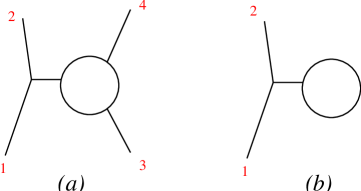
FIG. 4.: $(a)$ A 1-particle reducible graph. $(b)$ A graph with a tadpole subgraph.

A graph has tadpoles if it contains a subgraph from which stems a single line. It follows that all graphs with 1-point vertices have tadpoles. Obviously, when the single line of the tadpole is internal, the graph is 1-particle reducible (cf. figure 4$b$). An important particular case is that of actions for which $\langle\phi^{i}\rangle$ vanishes. This ensures that the effective current vanishes, i.e. $\overline{g}_{i}=0$ and thus all tree graphs of the theory “$\Gamma_{Q}+\Gamma_{I}$” are free of tadpoles (since tadpole subgraphs without 1-point vertices require at least one loop). Given any action, $\langle\phi^{i}\rangle=0$ can be achieved by a redefinition of the field $\phi^{i}$ by a constant shift, or else by a readjustment of the original current $g_{i}$, so this is usually a convenient choice. A further simplification can be achieved if $\Gamma_{Q}[\phi]$ is chosen as the full quadratic part of the effective action, so that $\overline{g}_{ij}$ vanishes. Under these two choices, each Green’s function requires only a finite number of tree graphs of the theory “$\Gamma_{Q}+\Gamma_{I}$”. Also, $\overline{s}^{ij}$ coincides with the full connected propagator, $G_{c}^{ij}$, since a single effective line is the only possible diagram for it. Up to 4-point functions, it is found

$$G_{c}^{i} = 0\,,$$ (13)

$$G_{c}^{ij} = \overline{s}^{ij}\,,$$ (14)

$$G_{c}^{ijk} = \overline{s}^{ia}\overline{s}^{jb}\overline{s}^{kc}\overline{g}_{abc}\,,$$ (15)

$$G_{c}^{ijk\ell} = \overline{s}^{ia}\overline{s}^{jb}\overline{s}^{kc}\overline{s}^{\ell d}\overline{g}_{abcd}$$ (17)

$$+\overline{s}^{ia}\overline{s}^{jb}\overline{g}_{abc}\overline{s}^{cd}\overline{g}_{def}\overline{s}^{ek}\overline{s}^{f\ell}+\overline{s}^{ia}\overline{s}^{kb}\overline{g}_{abc}\overline{s}^{cd}\overline{g}_{def}\overline{s}^{ej}\overline{s}^{f\ell}+\overline{s}^{ia}\overline{s}^{\ell b}\overline{g}_{abc}\overline{s}^{cd}\overline{g}_{def}\overline{s}^{ek}\overline{s}^{fj}\,.$$

The corresponding diagrams are depicted in figure 5. Previous considerations imply that in the absence of tadpoles, $G_{c}^{ij}=-((m+\Sigma)^{-1})^{ij}$.

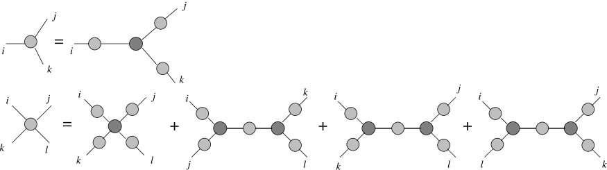
FIG. 5.: Feynman diagrams for the 3- and 4-point connected Green’s functions in terms of the proper functions (cf. eq. (14)). The lighter blobs represent the connected functions, the darker blobs represent the irreducible functions.

III Perturbation theory on non quadratic actions

A Statement of the problem and main result

All the previous statements are well known in the literature. Consider now the action $S[\phi]+\delta S[\phi]$, where

$$\delta S[\phi]=\sum_{n\geq 0}\frac{1}{n!}\delta g_{i_{1}\dots i_{n}}\phi^{i_{1}}\cdots\phi^{i_{n}}\,,$$ (18)

defines the perturbative vertices, $\delta g_{i_{1}\dots i_{n}}$. The above defined standard expansion to compute the full Green’s functions corresponds to the Feynman rules associated to the theory “$S_{Q}+(S_{I}+\delta S)$”, i.e., with $g_{i_{1}\cdots i_{n}}+\delta g_{i_{1}\cdots i_{n}}$ as new vertices. Equivalently, one can use an obvious generalization of the Feynman rules, using one kind of line, $s^{ij}$, and two kinds of vertices, $g_{i_{1}\dots i_{n}}$ and $\delta g_{i_{1}\dots i_{n}}$, which should be considered as distinguishable. As an alternative, we seek instead a diagrammatic calculation in terms of $\Gamma[\phi]$ and $\delta S[\phi]$, that is, using $\overline{s}^{ij}$ as line and $\overline{g}_{i_{1}\dots i_{n}}$ and $\delta g_{i_{1}\dots i_{n}}$ as vertices. The question of which new Feynman rules are to be used with these building blocks is answered by the following

Theorem. The Green’s functions associated to $S[\phi]+\delta S[\phi]$ follow from applying the Feynman rules of the theory “$\Gamma_{Q}+(\Gamma_{I}+\delta S)$” plus the further prescription of removing the graphs that contain “unperturbed loops”, i.e., loops constructed entirely from effective elements without any perturbative vertex $\delta g_{i_{1}\dots i_{n}}$.

This constitutes the basic result of this paper. The same statement holds in the presence of fermions. The proof is given below. We remark that the previous result does not depend on particular choices, such as $\overline{g}_{i}=\overline{g}_{ij}=0$. As a consistency check of the rules, we note that when $\delta S$ vanishes only tree level graphs of the theory “$\Gamma_{Q}+\Gamma_{I}$” remain, which is indeed the correct result. On the other hand, when $S[\phi]$ is quadratic, it coincides with its effective action (up to an irrelevant constant) and therefore there are no unperturbed loops to begin with. Thus, in this case our rules reduce to the ordinary ones. In this sense, the new rules given here are the general ones whereas the usual rules correspond only to the particular case of perturbing an action that is quadratic.

B Illustration of the new Feynman rules

To illustrate our rules, let us compute the corrections to the effective current and the self-energy, $\delta\overline{g}_{i}$ and $\delta\Sigma_{ij}$, induced by a perturbation at most quadratic in the fields, that is,

$$\delta S[\phi]=\delta g_{i}\phi^{i}+\frac{1}{2}\delta g_{ij}\phi^{i}\phi^{j}\,,$$ (19)

and at first order in the perturbation. To simplify the result, we will choose a vanishing $\overline{g}_{ij}$. On the other hand, $S_{Q}[\phi]$ will be kept fixed and $\delta S[\phi]$ will be included in the interacting part of the action, so $\delta\Sigma_{ij}=\delta\overline{m}_{ij}$.

Applying our rules, it follows that $\delta\overline{g}_{i}$ is given by the sum of 1-point diagrams of the theory “$\Gamma_{Q}+(\Gamma_{I}+\delta S)$” with either one $\delta g_{i}$ or one $\delta g_{ij}$ vertex and which are connected, amputated, 1-particle irreducible and contain no unperturbed loops. Likewise, $\delta\Sigma_{ij}$ is given by 2-point such diagrams. It is immediate that $\delta g_{i}$ can only appear in 0-loop graphs and $\delta g_{ij}$ can only appear in 0- or 1-loop graphs, since further loops would necessarily be unperturbed. The following result is thus found

$$\delta\overline{g}_{i} = \delta g_{i}+\frac{1}{2}\delta g_{ab}\overline{s}^{aj}\overline{s}^{bk}\overline{g}_{jki}\,,$$ (20)

$$\delta\Sigma_{ij} = \delta g_{ij}+\delta g_{ab}\overline{s}^{ak}\overline{s}^{b\ell}\overline{g}_{kni}\overline{g}_{\ell rj}\overline{s}^{nr}+\frac{1}{2}\delta g_{ab}\overline{s}^{ak}\overline{s}^{b\ell}\overline{g}_{k\ell ij}\,.$$ (21)

The graphs corresponding to the r.h.s. are shown in figure 6. There, the small full dots represent the perturbative vertices, the lines with lighter blobs represent the effective line and the vertices with darker blobs are the effective vertices. The meaning of this equation is, as usual, that upon expansion of the skeleton graphs in the r.h.s., every ordinary Feynman graph (i.e. those of the theory “$S_{Q}+(S_{I}+\delta S)$”) appears once and only once, and with the correct weight. In other words, the new graphs are a resummation of the old ones.

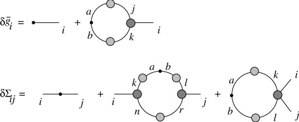
FIG. 6.: Diagrammatic representation of eqs. (21). The small full dot represents perturbation vertices. All graphs are amputated.

Let us take advantage of the above example to make several remarks. First, in order to use our rules, all $n$-point effective vertices have to be considered, in principle. In the example of figure 6, only the 3-point proper vertex is needed for the first order perturbation of the effective current and only the 3- and 4-point proper vertices are needed for the self-energy. Second, after the choice $\overline{g}_{ij}=0$, the corrections to any proper vertex requires only a finite number of diagrams, for any given order in each of the perturbation vertices $\delta g_{i_{1}\dots i_{n}}$. Finally, skeleton graphs with unperturbed loops should not be included. Consider, e.g. the graph in figure 7$a$. This graph contains an unperturbed loop. If its unperturbed loop is contracted to a single blob, this graph becomes the third 2-point graph in figure 6, therefore it is intuitively clear that it is redundant. In fact, the ordinary graphs obtained by expanding the blobs in figure 7$a$ in terms of “$S_{Q}+S_{I}$” are already be accounted for by the expansion of the third 2-point graph in figure 6.

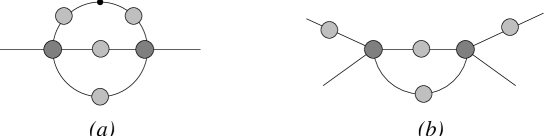
FIG. 7.: $(a)$ A redundant graph. Meaning of lines and vertices as in figures 5 and  6. $(b)$ The associated unperturbed graph to $(a)$.

For a complicated diagram of the theory “$\Gamma_{Q}+(\Gamma_{I}+\delta S)$”, the cleanest way to check for unperturbed loops is to construct its associated unperturbed graph. This is the graph of the theory “$\Gamma_{Q}+\Gamma_{I}$” which is obtained after deleting all perturbation vertices, so that the ends previously attached to such vertices become external legs in the new graph. Algebraically this means to remove the $\delta g_{i_{1}\dots i_{n}}$ factors so that the involved indices become external (uncontracted) indices. The number of unperturbed loops of the old (perturbed) graph coincides the number of loops of the associated unperturbed graph. The associated graph to that in figure 7$a$ is depicted in figure 7$b$.

IV Some applications

Of course, the success of the standard Feynman diagrammatic technique is based on the fact that quadratic actions, unlike non quadratic ones, can be easily and fully solved. Nevertheless, even when the theory $S[\phi]$ is not fully solved, our expansion can be useful. First, it helps in organizing the calculation. Indeed, in the standard expansion the same 1-, 2-,…, $n$-point unperturbed Green’s functions are computed over and over, as subgraphs, instead of only once. Second, and related, because the perturbative expansion in $S_{I}[\phi]$ must be truncated, in the standard expansion one is in general using different approximations for the same Green’s functions of $S[\phi]$ in different subgraphs. As a consequence, some known exact properties (such as symmetries, experimental values of masses or coupling constants, etc) of the Green’s functions of $S[\phi]$ can be violated by the standard calculation. On the contrary, in the expansion proposed here, the Green’s functions of $S[\phi]$ are taken as an input and hence one can make approximations to them (not necessarily perturbative) to enforce their known exact properties. As an example consider the Casimir effect. The physical effect of the conductors is to change the photon boundary conditions. This in turn corresponds to modify the free photon propagator [7], i.e., to add a quadratic perturbation to the Lagrangian of quantum electrodynamics (QED). Therefore our expansion applies. The advantage of using it is that one can first write down rigorous relations (perturbative in $\delta S$ but non perturbative from the point of view of QED) and, in a second step, the required QED propagators and vertex functions can be approximated (either perturbatively or by some other approach) in a way that is consistent with the experimentally known mass, charge and magnetic moment of the electron, for instance. Another example would be chiral perturbation theory: given some approximation to massless Quantum Chromodynamics (QCD), the corrections induced by the finite current quark masses can be incorporated using our scheme as a quadratic perturbation. Other examples would be the corrections induced by a non vanishing temperature or density, both modifying the propagator.

A Derivation of diagrammatic identities

Another type of applications comes in the derivation of diagrammatic identities. We can illustrate this point with some Schwinger-Dyson equations [1, 2, 3]. Let $\epsilon^{i}$ be field independent. Then, noting that the action $S[\phi+\epsilon]$ has $\Gamma[\phi+\epsilon]$ as its effective action, and for infinitesimal $\epsilon^{i}$, it follows that the perturbation $\delta S[\phi]=\epsilon^{i}\partial_{i}S[\phi]$ yields a corresponding correction $\delta\Gamma[\phi]=\epsilon^{i}\partial_{i}\Gamma[\phi]$ in the effective action. Therefore for this variation we can write:

$$\delta\overline{g}_{i} = \delta\partial_{i}\Gamma[0]=\epsilon^{j}\partial_{i}\partial_{j}\Gamma[0]=\epsilon^{j}(m+\Sigma)_{ij}\,,$$ (22)

$$\delta\Sigma_{ij} = \delta\partial_{i}\partial_{j}\Gamma[0]=\epsilon^{k}\partial_{i}\partial_{j}\partial_{k}\Gamma[0]=\epsilon^{k}\overline{g}_{ijk}\,.$$ (23)

Let us particularize to a theory with a 3-point bare vertex, then $\delta S[\phi]$ is at most a quadratic perturbation with vertices $\delta g_{j}=\epsilon^{i}(m_{ij}+g_{ij})$ and $\delta g_{jk}=\epsilon^{i}g_{ijk}$. Now we can immediately apply eqs. (21) to obtain the well known Schwinger-Dyson equations

$$\Sigma_{ij} = g_{ij}+\frac{1}{2}g_{iab}\bar{s}^{a\ell}\bar{s}^{br}\bar{g}_{\ell rj}\,,$$ (24)

$$\overline{g}_{cij} = g_{cij}+g_{cab}\overline{s}^{ak}\overline{s}^{b\ell}\overline{g}_{kni}\overline{g}_{\ell rj}\overline{s}^{nr}+\frac{1}{2}g_{cab}\overline{s}^{ak}\overline{s}^{b\ell}\overline{g}_{k\ell ij}\,.$$ (25)

The corresponding diagrams are depicted in figure 8.

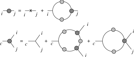
FIG. 8.: Two Schwinger-Dyson equations for a cubic action.

B Effective Lagrangians and the double-counting problem

There are instances in which we do not have (or is not practical to use) the underlying unperturbed action and we are provided directly, through the experiment, with the Green’s functions. In these cases it is necessary to know which Feynman rules to use with the exact Green’s functions of $S$. Consider for instance the propagation of particles in nuclear matter. This is usually described by means of so called effective Lagrangians involving the nucleon field and other relevant degrees of freedom (mesons, resonances, photons, etc). These Lagrangians are adjusted to reproduce at tree level the experimental masses and coupling constants. (Of course, they have to be supplemented with form factors for the vertices, widths for the resonances, etc, to give a realistic description, see e.g. [8].) Thus they are a phenomenological approximation to the effective action rather than to the underlying bare action $S$. So to say, Nature has solved the unperturbed theory (in this case the vacuum theory) for us and one can make experimental statements on the exact (non perturbative) Green’s functions. The effect of the nuclear medium is accounted for by means of a Pauli blocking correction to the nucleon propagator in the vacuum, namely,

$$G(p) = (p^{0}-\epsilon(\vec{p})+i\eta)^{-1}+2i\pi n(\vec{p})\delta(p^{0}-\epsilon(\vec{p}))=G_{0}(p)+\delta G(p)\,,$$ (26)

where $G_{0}(p)$ and $G(p)$ stand for the nucleon propagator at vacuum and at finite density, respectively, $n(\vec{p})$ is the Fermi sea occupation number and $\epsilon(\vec{p})$ is the nucleon kinetic energy. In the present case, the vacuum theory is the unperturbed one whereas the Pauli blocking correction is a 2-point perturbation to the action and our expansion takes the form of a density expansion.

The use of an effective Lagrangian, instead of a more fundamental one, allows to perform calculations in terms of physical quantities and this makes the phenomenological interpretation more direct. However, the use of the standard Feynman rules is not really justified since they apply to the action and not to the effective action, to which the effective Lagrangian is an approximation. A manifestation of this problem comes in the form of double-counting of vacuum contributions, which has to be carefully avoided. This is obvious already in the simplest cases. Consider, for instance, the nucleon self-energy coming from exchange of virtual pions, with corresponding Feynman graph depicted in figure 9$a$. This graph gives a non vanishing contribution even at zero density. Such vacuum contribution is spurious since it is already accounted for in the physical mass of the nucleon. The standard procedure in this simple case is to subtract the same graph at zero density in order to keep the true self-energy. This is equivalent to drop $G_{0}(p)$ in the internal nucleon propagator and keep only the Pauli blocking correction $\delta G(p)$. In more complicated cases simple overall subtraction does not suffice, as it is well known from renormalization theory; there can be similar spurious contributions in subgraphs even if the graph vanishes at zero density. An example is shown in the photon self-energy graph of figure 9$b$. The vertex correction subgraphs contain a purely vacuum contribution that is already accounted for in the effective $\gamma NN$ vertex. Although such contributions vanish if the exchanged pion is static, they do not in general. As is clear from our theorem, the spurious contributions are avoided by not allowing vacuum loops in the graphs. That is, for each standard graph consider all the graphs obtained by substituting each $G(p)$ by either $G_{0}(p)$ or $\delta G(p)$ and drop all graphs with any purely vacuum loop. We emphasize that strictly speaking the full propagator and the full proper vertices of the vacuum theory have to be used to construct the diagrams. In each particular application it is to be decided whether a certain effective Lagrangian (plus form factors, widths, etc) is a sufficiently good approximation to the effective action.

FIG. 9.: Nucleon (a) and photon (b) self-energy diagrams.

C Derivation of low density theorems

A related application of our rules comes from deriving low density theorems. For instance, consider the propagation of pions in nuclear matter and in particular the pionic self-energy at lowest order in an expansion on the nuclear density. To this end one can use the first order correction to the self-energy as given in eq. (21), when the labels $i,j$ refer to pions and the 2-point perturbation is the Pauli blocking correction for the nucleons. Thus, the labels $a,b,k,\ell$ (cf. second line of figure 6) necessarily refer to nucleons whereas $n,r$ can be arbitrary baryons ($B$). In this case, the first 2-point diagram in figure 6 vanishes since $i,j$ are pionic labels which do not have Pauli blocking. On the other hand, as the nuclear density goes to zero, higher order diagrams (i.e. with more than one full dot, not present in figure 6) are suppressed and the second and third 2-point diagrams are the leading contributions to the pion self energy. The $\pi NB$ and $\pi\pi NN$ proper vertices in these two graphs combine to yield the $\pi N$ $T$-matrix, as is clear by cutting the corresponding graphs by the full dots. (Note that the Dirac delta in the Pauli blocking term places the nucleons on mass shell.) We thus arrive at the following low density theorem [9]: at lowest order in a density expansion in nuclear matter, the pion optical potential is given by the nuclear density times the $\pi N$ forward scattering amplitude. This result holds independently of the detailed pion-nucleon interaction and regardless of the existence of other kind of particles as well since they are accounted for by the $T$-matrix.

D Applications to non perturbative renormalization in Quantum Field Theory

Let us consider a further application, this time to the problem of renormalization in Quantum Field Theory (QFT). To be specific we consider the problem of ultraviolet divergences. To first order in $\delta S$, our rules can be written as

$$\delta\Gamma[\phi]=\langle\delta S\rangle^{\phi}\,,$$ (27)

where $\langle A\rangle^{\phi}$ means the expectation value of $A[\phi]$ in the presence of an external current $J$ tuned to yield $\phi$ as the expectation value of the field. This formula is most simply derived directly from the definitions give above. (In passing, let us note that this formula defines a group of transformations in the space of actions, i.e., unlike standard perturbation theory, it preserves its form at any point in that space.) We can consider a family of actions, taking the generalized coupling constants as parameters, and integrate the above first order evolution equation taking e.g. a quadratic action as starting point. Perturbation theory corresponds to a Taylor expansion solution of this equation.

To use this idea in QFT, note that our rules directly apply to any pair of regularized bare actions $S$ and $S+\delta S$. Bare means that $S$ and $S+\delta S$ are the true actions that yield the expectation values in the most naive sense and regularized means that the cut off is in place so that everything is finite and well defined. As it is well known, a parametric family of actions is said to be renormalizable if the parameters can be given a suitable dependence on the cut off so that all expectation values remain finite in the limit of large cut off (and the final action is non trivial, i.e., non quadratic). In this case the effective action has also a finite limit. Since there is no reason to use the same cut off for $S$ and $\delta S$, we can effectively take the infinite cut off limit in $\Gamma$ keeping finite that of $\delta S$. (For instance, we can regularize the actions by introducing some non locality in the vertices and taking the local limit at different rates for both actions.) So when using eq. (27), we will find diagrams with renormalized effective lines and vertices from $\Gamma$ and bare regularized vertices from $\delta S$. Because $\delta\Gamma$ is also finite as the cut off is removed, it follows that the divergences introduced by $\delta S$ should cancel with those introduced by the loops. This allows to restate the renormalizability of a family of actions as the problem of showing that 1) assuming a given asymptotic behaviour for $\Gamma$ at large momenta, the parameters in $\delta S$ can be given a suitable dependence on the cut off so that $\delta\Gamma$ remains finite, 2) the assumed asymptotic behaviour is consistent with the initial condition (e.g. a free theory) and 3) this asymptotic behaviour is preserved by the evolution equation. This would be an alternative to the usual forest formula analysis which would not depend on perturbation theory. If the above program were successfully carried out (the guessing of the correct asymptotic behaviour being the most difficult part) it would allow to write a renormalized version of the evolution equation (27) and no further renormalizations would be needed. (Related ideas regarding evolution equations exist in the context of low momenta expansion, see e.g. [10] or to study finite temperature QFT [11].)

To give an (extremely simplified) illustration of these ideas, let us consider the family of theories with Euclidean action

$$S[\phi,\psi]=\int d^{4}x\left(\frac{1}{2}(\partial\phi)^{2}+\frac{1}{2}m^{2}\phi^{2}+\frac{1}{2}(\partial\psi)^{2}+\frac{1}{2}M^{2}\psi^{2}+\frac{1}{2}g\phi\psi^{2}+h\phi+c\right).$$ (28)

Here $\phi(x)$ and $\psi(x)$ are bosonic fields in four dimensions. Further, we will consider only the approximation of no $\phi$-propagators inside of loops. This approximation, which treats the field $\phi$ at a quasi-classical level, is often made in the literature. It As it turns out, the corresponding evolution equation is consistent, that is, the right-hand side of eq. (27) is still an exact differential after truncation. In order to evolve the theory we will consider variations in $g$, and also in $c$, $h$ and $m^{2}$, since these latter parameters require a ($g$-dependent) renormalization. (There are no field, $\psi$-mass or coupling constant renormalization in this approximation.) That is

$$\delta S[\phi,\psi]=\int d^{4}x\left(\frac{1}{2}\delta m^{2}\phi^{2}+\frac{1}{2}\delta g\phi\psi^{2}+\delta h\phi+\delta c\right)\,.$$ (29)

The graphs with zero and one $\phi$-leg are divergent and clearly they are renormalized by $\delta c$ and $\delta h$, so we concentrate on the remaining divergent graph, namely, that with two $\phi$-legs. Noting that in this quasi-classical approximation $g$ coincides with the full effective coupling constant and $S_{\psi}(q)=(q^{2}+M^{2})^{-1}$ coincides with the the full propagator of $\psi$, an application of the rules gives (cf. figure 10)

$$\delta\Sigma_{\phi}(k)=\delta m^{2}-\delta gg\int\frac{d^{4}q}{(2\pi)^{4}}\theta(\Lambda^{2}-q^{2})S_{\psi}(q)S_{\psi}(k-q)\,,$$ (30)

where $\Lambda$ is a sharp ultraviolet cut off.

FIG. 10.: Diagrammatic representation of eq. (30).

Let us denote the cut off integral by $I(k^{2},\Lambda^{2})$. This integral diverges as $\frac{1}{(4\pi)^{2}}\log(\Lambda^{2})$ for large $\Lambda$ and fixed $k$. Hence $\delta\Sigma_{\phi}$ is guaranteed to remain finite if, for large $\Lambda$, $\delta m^{2}$ is taken in the form

$$\delta m^{2}=\delta m_{R}^{2}+\delta gg\frac{1}{(4\pi)^{2}}\log(\Lambda^{2}/\mu^{2})$$ (31)

where $\mu$ is an arbitrary scale (cut off independent), and $\delta m_{R}^{2}$ is an arbitrary variation. Thus, the evolution equation for large cut off can be written in finite form, that is, as a renormalized evolution equation, as follows

$$\delta\Sigma_{\phi}(k)=\delta m_{R}^{2}-\delta ggI_{R}(k^{2},\mu^{2})\,,$$ (32)

where

$$I_{R}(k^{2},\mu^{2})=\lim_{\Lambda\to\infty}\left(I(k^{2},\Lambda^{2})-\frac{1}{(4\pi)^{2}}\log(\Lambda^{2}/\mu^{2})\right)\,.$$ (33)

Here $\delta g$ and $\delta m_{R}^{2}$ are independent and arbitrary ultraviolet finite variations. The physics remains constant if a different choice of $\mu$ is compensated by a corresponding change in $\delta m_{R}^{2}$ so that $\delta m^{2}$, and hence the bare regularized action, is unchanged. The essential point has been that $\delta m^{2}$ could be chosen $\Lambda$ dependent but $k^{2}$ independent. As mentioned, this example is too simple since it hardly differs from standard perturbation theory. The study of the general case (beyond quasi-classical approximations) with this or other actions seems very interesting from the point of view of renormalization theory.

V Proof of the theorem

In order to prove the theorem it will be convenient to change the notation: we will denote the unperturbed action by $S_{0}[\phi]$ and its effective action by $\Gamma_{0}[\phi]$. The generating function of the full perturbed system is

$$Z[J]=\int\exp\left(S_{0}[\phi]+\delta S[\phi]+J\phi\right)\,d\phi\,.$$ (34)

By definition of the effective action, the connected generating function of the unperturbed theory is

$$W_{0}[J]=\max_{\phi}\left(\Gamma_{0}[\phi]+J\phi\right)\,,$$ (35)

thus, up to a constant ($J$-independent) factor, we can write

$$\exp\left(W_{0}[J]\right) = \lim_{\hbar\to 0}\left[\int\exp\left(\hbar^{-1}\left(\Gamma_{0}[\phi]+J\phi\right)\right)\,d\phi\right]^{\textstyle\hbar}\,.$$ (36)

$\hbar$ is merely a bookkeeping parameter here which is often used to organize the loop expansion [12, 5]. The $\hbar$-th power above can be produced by means of the replica method [5]. To this end we introduce a number $\hbar$ of replicas of the original field, which will be distinguished by a new label $k$. Thus, the previous equation can be rewritten as

$$\exp\left(W_{0}[J]\right)=\lim_{\hbar\to 0}\int\exp\left(\hbar^{-1}\sum_{k}\left(\Gamma_{0}[\phi_{k}]+J\phi_{k}\right)\right)\prod_{k}d\phi_{k}\,.$$ (37)

On the other hand, the identity (up to a constant) $\int\exp\left(J\phi\right)\,d\phi=\delta[J]$, where $\delta[J]$ stands for a Dirac delta, allows to write the reciprocal relation of eq. (8), namely

$$\exp\left(S_{0}[\phi]\right)=\int\exp\left(W_{0}[J_{0}]-J_{0}\phi\right)\,dJ_{0}\,.$$ (38)

If we now use eq. (37) for $\exp W_{0}$ in eq. (38) and the result is substituted in eq. (34), we obtain

$$Z[J]=\lim_{\hbar\to 0}\int\exp\left(\hbar^{-1}\sum_{k}\left(\Gamma_{0}[\phi_{k}]+J_{0}\phi_{k}\right)+\delta S[\phi]+\left(J-J_{0}\right)\phi\right)\,dJ_{0}\,d\phi\prod_{k}d\phi_{k}\,.$$ (39)

The integration over $J_{0}$ is immediate and yields a Dirac delta for the variable $\phi$, which allows to carry out also this integration. Finally the following formula is obtained:

$$Z[J]=\lim_{\hbar\to 0}\int\exp\left(\hbar^{-1}\sum_{k}\left(\Gamma_{0}[\phi_{k}]+J\phi_{k}\right)+\delta S\big{[}\hbar^{-1}\sum_{k}\phi_{k}\big{]}\right)\prod_{k}d\phi_{k}\,.$$ (40)

which expresses $Z[J]$ in terms of $\Gamma_{0}$ and $\delta S$. Except for the presence of replicas and explicit $\hbar$ factors, this formula has the same form as that in eq. (34) and hence it yields the same standard Feynman rules but with effective lines and vertices.

Consider any diagram of the theory “$\Gamma_{Q}+(\Gamma_{I}+\delta S)$”, as described by eq. (40) before taking the limit $\hbar\to 0$. Let us now show that such diagram carries precisely a factor $\hbar^{L_{0}}$, where $L_{0}$ is the number of unperturbed loops in the graph. Let $P$ be the total number of lines (both internal and external), $E$ the number of legs, $L$ the number of loops and $C$ the number of connected components of the graph. Furthermore, let $V^{0}_{n}$ and $\delta V_{n}$ denote the number of $n$-point vertices of the types $\Gamma_{0}$ and $\delta S$ respectively. After these definitions, let us first count the number of $\hbar$ factors coming from the explicit $\hbar^{-1}$ in eq. (40). The arguments are standard [12, 3, 5]: from the Feynman rules it is clear that each $\Gamma_{0}$ vertex carries a factor $\hbar^{-1}$, each effective propagator carries a factor $\hbar$ (since it is the inverse of the quadratic part of the action), each $n$-point $\delta S$ vertex carries a factor $\hbar^{-n}$ and each leg a $\hbar^{-1}$ factor (since they are associated to the external current $J$). That is, this number is

$$N_{0}=P-\sum_{n\geq 0}V^{0}_{n}-E-\sum_{n\geq 0}n\delta V_{n}\,.$$ (41)

Recall now the definition given above of the associated unperturbed diagram, obtained after deleting all perturbation vertices, and let $P_{0}$, $E_{0}$, $L_{0}$ and $C_{0}$ denote the corresponding quantities for such unperturbed graph. Note that the two definitions given for the quantity $L_{0}$ coincide. Due to its definition, $P_{0}=P$ and also $E_{0}=E+\sum_{n\geq 0}n\delta V_{n}$, this allows to rewrite $N_{0}$ as

$$N_{0}=P_{0}-\sum_{n\geq 0}V^{0}_{n}-E_{0}\,.$$ (42)

Since all quantities now refer a to the unperturbed graph, use can be made of the well known diagrammatic identity $N_{0}=L_{0}-C_{0}$. Thus from the explicit $\hbar$, the graph picks up a factor $\hbar^{L_{0}-C_{0}}$. Let us now turn to the implicit $\hbar$ dependence coming from the number of replicas. The replica method idea applies here directly: because all the replicas are identical, summation over each different free replica label in the diagram yields precisely one $\hbar$ factor. From the Feynman rules corresponding to the theory of eq. (40) it is clear that all lines connected through $\Gamma_{0}$ vertices are constrained to have the same replica label, whereas the coupling through $\delta S$ vertices does not impose any conservation law of the replica label. Thus, the number of different replica labels in the graph coincides with $C_{0}$. In this argument is is essential to note that the external current $J_{i}$ has not been replicated; it couples equally to all the replicas. Combining this result with that previously obtained, we find that the total $\hbar$ dependence of a graph goes as $\hbar^{L_{0}}$. As a consequence, all graphs with unperturbed loops are removed after taking the limit $\hbar\to 0$. This establishes the theorem.

Some remarks can be made at this point. First, it may be noted that some of the manipulations carried out in the derivation of eq. (40) were merely formal (beginning by the very definition of the effective action, since there could be more than one extremum in the Legendre transformation), however they are completely sufficient at the perturbative level. Indeed, order by order in perturbation theory, the unperturbed action $S_{0}[\phi]$ can be expressed in terms of its effective action $\Gamma_{0}[\phi]$, hence the Green’s functions of the full theory can be expressed perturbatively within the diagrams of the theory “$\Gamma_{Q}+(\Gamma_{I}+\delta S)$”. It only remains to determine the weighting factor of each graph which by construction (i.e. the order by order inversion) will be just a rational number. Second, it is clear that the manipulations that lead to eq. (40) can be carried out in the presence of fermions as well, and the same conclusion applies. Third, note that in passing, it has been proven also the statement that the effective action yields at tree level the same Green’s functions as the bare action at all orders in the loop expansion, since this merely corresponds to set $\delta S[\phi]$ to zero. Finally, eq. (40) does not depend on any particular choice, such as fixing $\langle\phi^{i}\rangle=0$ to remove tadpole subgraphs.

REFERENCES

- [1] Dyson F J 1949 Phys. Rev. 75 1736.
- [2] Schwinger J 1951 Proc. Natl. Acad. Sci. U.S.A. 35 452.
- [3] Itzykson C and Zuber J B 1980 Quantum Field Theory (New York: McGraw-Hill.)
- [4] Iliopoulos J, Itzykson C and Martin A 1975 Rev. Mod. Phys. 47 165.
- [5] Negele J W and Orland H 1988 Quantum many-particle systems (Redwood City, Calif.: Addison-Wesley Pub. Co.)
- [6] Cornwall J M, Jackiw R and Tomboulis E 1974 Phys. Rev. D10 2428.
- [7] Bordag M, Robaschik D and Wieczorek E 1985 Ann. Phys. (N.Y.) 165 192.
- [8] Ericson T E O and Weise W 1988 Pions and nuclei (Oxford: Clarendon Press, New York: Oxford University Press)
- [9] Hüfner J 1975 Phys. Reports 21 1.
- [10] Morris T R 1996 Nucl.Phys. B458 477.
- [11] D’Attanasio M D and Pietroni M 1996, Nucl.Phys. B472 711.
- [12] Coleman S and Weinberg E 1973 Phys. Rev. D7 1888.