Quantum Chrono-Topology of Nuclear and Sub-Nuclear Reactions

Abstract

A quantum time topological space is developed and applied to solve some problems about quantum theory. It is disconnected and satifies the separation axioms of ${\cal T}_{4}$. The degree of disconnectedness of the time-space is a decreasing function of the number of simultaneous or almost simultaneous fundamental interactions. The disconnectedness of the $\kappa\times\lambda_{\kappa}$-fold time-space, ${\cal T}_{4}^{\kappa\lambda_{\kappa}}$, imparts a quantization to $\kappa\times\lambda_{\kappa}$-fold space-time, $\bar{M}^{4}_{\kappa\lambda_{\kappa}}$, and induces it’s topology. In this topology the ${\bf U}+{\bf R}$ Penrose dynamics is implemented by means of a time evolution operator, ${\cal U}$, in QFT. $\cal U$ is unitary or non-unitary, depending on the type of quantization of the field action-integral. ${\cal U}$ allows to find the Boltzmann factor in QFT in the above space-time. From an elementary solution of the Liouville equation the quantization of the time follows and the Planck constant has been calculated. Compatibility between time-reversal and irreversibility is spontaneously obtained. The renormalization of the field action-integral follows from quantization. The solution of the measurement problem and the wave function reduction have been deduced in the framework of the Schroedinger theory. The Schroedinger cat’s paradoxon and the paradoxon of the wave paket decay have been resolved.

1 Introduction

Indications that systems of atomic, nuclear and sub-nuclear particles cannot have the topology of the Newtonian time ($\mathchoice{\displaystyle{I\mkern-6.0muR}}{\textstyle{I\mkern-6.0muR}}{\scriptstyle{I\mkern-6.0muR}}{\scriptscriptstyle{I\mkern-6.0muR}}^{1}$) were available as early as in 1974 [1]. It became clear that quanta need not take notice of any observers except interactions with other quanta or particles. What is time for the quanta? What is its nature? Why should quanta take notice of the time defined by observers of their behavior? If at all, should not particles have their own times? The question about the time is a very old one. Nevertheless, a definitive answer has not been obtained sofar.

The increasing number of paradoxes in theoretical physics generally and in nuclear and sub-nuclear theory in particular, while the experimental quantum techniques become more and more sophisticated and of higher accuracy, imposes increasingly the view that something about the fundamental physical concepts should be revised.

A systematic examination showed that most uncertainty in physics is associated with the time concept. This variable, being interwoven with the space through relativity, imposes its topology to the space-time, and it determines, in this way, the evolution in the nuclear and sub-nuclear interactions among others.

We propose a new space-time topology, the Chrono-topology. It is based on the concept of the Interaction Proper-time Neighbourhood, $\tau$, (IPN). The space-time topology on the quantum level is determined by the number of the interacting particles in every particular system. For small numbers of interacting particles the new time-space is a ${\cal T}_{4}$ topological space.

The new space-times, $\bar{M^{4}_{\kappa\lambda}}$ being in general $\kappa\times\lambda$-fold in time, are defined as the Cartesian products, $\mathchoice{\displaystyle{I\mkern-6.0muR}}{\textstyle{I\mkern-6.0muR}}{\scriptstyle{I\mkern-6.0muR}}{\scriptscriptstyle{I\mkern-6.0muR}}^{3}\times{\cal T}^{\kappa\lambda}_{4}$, of ${\cal T}^{\kappa\lambda}_{4}$. The latter is a $\kappa\times\lambda$-fold, disconnected topological space satisfying the separation axioms of a ${\cal T}_{4}$ space whose elements are the interaction proper-time neighbourhoods, $\{\tau_{\lambda}|\forall\lambda\mathrel{\mathchoice{\raise 0.86108pt\hbox{$\scriptstyle\in$}}{\raise 0.86108pt\hbox{$\scriptstyle\in$}}{\raise 0.86108pt\hbox{$\scriptscriptstyle\in$}}{\raise 0.86108pt\hbox{$\scriptscriptstyle\in$}}}\mathchoice{{\sevenrm Z}\mkern-9.2mu{\sevenrm Z}}{{\sevenrm Z}\mkern-9.2mu{\sevenrm Z}}{{\sevenrm Z}\mkern-9.2mu{\sevenrm Z}}{{\sevenrm Z}\mkern-9.2mu{\sevenrm Z}}^{+}\}$.

Our $\bar{M^{4}}$ is not related to Hawking’s space-time foam [24] neither as to the cell magnitude nor as to its creation process. While Hawking explains, as does Wheeler [14] the space-time foam creation by means of the field fluctuations in Planck time scale, our $\bar{M^{4}}$ is due to changes of physical observables caused by fundamental interactions and mapped into a definite IPN in each one case.

Although we do not discuss General Relativity in this work, we feel, knowing the results of our chrono-topology, that General Relativity, being based on the Newtonian time topology, is per construction a non-quantizable theory, and that a reformulation of the field equations in the framework of chrono-topology may lead to a quantum theory of space-time whose average will give for macroscopic space-time neighorhoods the Einstein field equations of gravity.

1.1 Hunting the trace of the time

Many famous authors have been occupied with the answering the question about the nature of time as: Aristotle [2], Newton [3], Kant [4], Bergson [5], and many others. The searching for the meaning of the time by the above Researchers and Philosophers was rather of a knowledge theoretical character, such that no direct physical judgement - except a logical one - of the practical applicability to modern problems in physics was possible. Also, Eddington [6], Whitehead [7], Einstein [8], Dirac [9], and particularly Prigogine [10], Wheeler [14] and others have shown a deep concern in the elucidation of the nature and properties of time. Their search for the meaning of time was of such a character that the results obtained on the basis of its structure were accessible to a certain extent to a kind of physical verification.

It is extremely interesting to verify, after a debate of long decades, Einstein’s terrifically strong insight: Now we know that, in fact, ”Gott wuerfelt nicht” - God does not play dice in matters of quantum theory.

It will be shown that quantum mechanics is, in fact, per se not a statistical theory inside an IPN. The statistical character is imposed on the wave function by the topology of the space-time $\bar{M^{4}_{\kappa\lambda_{\kappa}}}$, not by the Minkowski space-time, $M^{4}$.

Meanwhile, new problems appeared mainly in theoretical physics which are not solvable in the frame of the current understanding of time’s nature. Bell [11], Hawking [12], Penrose [15], Unruh [16], Stamp [17], Legget [18], Douglas [19] have published important works on this area. Nevertheless, the time issue remained still open.

The beautiful researches of all above and many other authors [20]-[31] are only a very small sample of the world literature on time’s nature. However, there still exist very seriously resisting problems in particular in quantum theory which make this issue central to the atomic, to the nuclear and to the elementary particles theoretical physics [32]- [41].

1.2 Annoying questions

Spectacularly successful results have been achieved in these areas of physics during our century, and a high degree of maturity both in experiment and in theory. Nevertheless, the nature of time was still unclear and very important questions remained open:

1. Can we understand the wave packet’s decay in absence of interactions.

2. Can we understand the reduction of the wave function in the framework of the Schroedinger equation?

3. Can we derive rigorously quantum statistical mechanics (QSM), in particular, the Boltzmann factor from quantum field theory (QFT)?

4. Can we explain the microscopic and the macroscopic irreversibility of many phenomena starting from QFT?

5. Why is there a tunnel effect?

6. Why is there an ergodicity?

7. Why is there a Poincare returning.

8. Why quarks are not directly observable?

9. Have the non-locality, related to the Bell theory [42], and the interpretation of the Aspect et al. experiment [43] to do with the topology of the time?, etc, etc, $\ldots$.

After the discovery of Einstein’s relativity it became clear by the Lorentz transformation that time and space are interwoven in the Minkowski space-time, $M^{4}$. Another important recognition provided by relativity was that each 3-space point is associated with its own time (event), the proper-time.

Accordingly, one would expect that these facts should, normally, impose the replacement in modern physics of the universal Newtonian time by the new Einsteinian time. This would make justice to Dirac’s early proposal [9] that every particle in the many-particle Schroedinger equation should have its own time variable. Dirac’s proposal, being related to the topology of the space-time has not yet found the place in physics which it deserves.

To shed some light on a few aspects of the above problems of paramount importance for the future physics is the hope and the purpose of the present work.

1.3 The mighty Newton

It is important to note that, whichever is the topology adopted for the time, a transformation like

$$\{x^{\prime}=L_{x}(x,t),t^{\prime}=L_{t}(x,t)\},\>x\mathrel{\mathchoice{\raise 0.86108pt\hbox{$\scriptstyle\in$}}{\raise 0.86108pt\hbox{$\scriptstyle\in$}}{\raise 0.86108pt\hbox{$\scriptscriptstyle\in$}}{\raise 0.86108pt\hbox{$\scriptscriptstyle\in$}}}X\subset\mathchoice{\displaystyle{I\mkern-6.0muR}}{\textstyle{I\mkern-6.0muR}}{\scriptstyle{I\mkern-6.0muR}}{\scriptscriptstyle{I\mkern-6.0muR}}^{1}$$ (1.1)

induces on the Minkowski space, the Cartesian product space $M^{4}=i\mathchoice{\displaystyle{I\mkern-6.0muR}}{\textstyle{I\mkern-6.0muR}}{\scriptstyle{I\mkern-6.0muR}}{\scriptscriptstyle{I\mkern-6.0muR}}^{1}\times\mathchoice{\displaystyle{I\mkern-6.0muR}}{\textstyle{I\mkern-6.0muR}}{\scriptstyle{I\mkern-6.0muR}}{\scriptscriptstyle{I\mkern-6.0muR}}^{3}$, the topology of that time.

In the same way the Lorentz transformation $(x,t)\to(x^{\prime},t^{\prime})$ induces the topology of the Newtonian time, $t$, on each space point, $x^{\prime}$, in the neighbourhood associated with that time, $t$, and space point, $x$.

Space-time topologies resulting from solutions of the Einstein field equations will be mentioned here only occasionally. However, we cannot tacitly bypass the fact that in general relativity the proper-time is a function of the Newtonian time. For example, in the Schwartzschild metric

$$ds^{2}=c^{2}(1-\frac{r_{g}}{r})dt^{2}-r^{2}(\sin\theta d\phi+d\theta^{2})-\frac{dr^{2}}{1-\frac{r_{g}}{r}},$$ (1.2)

the time variable takes values as $t\mathrel{\mathchoice{\raise 0.86108pt\hbox{$\scriptstyle\in$}}{\raise 0.86108pt\hbox{$\scriptstyle\in$}}{\raise 0.86108pt\hbox{$\scriptscriptstyle\in$}}{\raise 0.86108pt\hbox{$\scriptscriptstyle\in$}}}T=\mathchoice{\displaystyle{I\mkern-6.0muR}}{\textstyle{I\mkern-6.0muR}}{\scriptstyle{I\mkern-6.0muR}}{\scriptscriptstyle{I\mkern-6.0muR}}^{1}$ [45].

Also in the general relativity, for example [46], one reads: ”Any monotonic parameter, increasing from the past to the future (i.e. $t\mathrel{\mathchoice{\raise 0.86108pt\hbox{$\scriptstyle\in$}}{\raise 0.86108pt\hbox{$\scriptstyle\in$}}{\raise 0.86108pt\hbox{$\scriptscriptstyle\in$}}{\raise 0.86108pt\hbox{$\scriptscriptstyle\in$}}}[-\infty,+\infty]$) might be used to measure time on the world line of a material particle”. This is clearly correct for a macroscopic theory. Is it correct for the discontinuous quantum phenomena?

Nevertheless, this attitude reflects the view of some researchers according to which time had nothing to do with the fundamental interactions and with the changes induced by them in the different neighbourhoods of the universe.

This attitude is rejected in the present work.

1.4 Quanta and their self-determination - The interaction proper-time neighbourhood (IPN)

In view of these facts one may speculate, if not reasonably conjecture, that the well-known paradoxes in relativity and quantum theory, as well as the possibility for their appearance in physical theories are due to the space-time topology imposed by the Newtonian time.

Despite the obvious necessity to replace the Newtonian time and its topology by IPNs to be defined precisely below for each event, the Newtonian time remaines until today generally dominant in classical and in quantum theory.

The present paper is dealing with the derivation of some consequences of a new type of time topology discovered earlier [1] and taken as the basis in this work. The new topology derives from the fundamental observation teaching us that no time would be definable, if nothing changed in the universe [48].

Since the universe for a non-interacting, structureless particle is the particle itself, no time exists for it. Moreover, since the nuclear and sub-nuclear interactions factually are, each one, of finite duration, i.e., they are related to finite changes of the observables involved in the interaction, it is clear that IPN cannot be identified with the Newtonian time. Because the latter is homeomorphic to the whole $\mathchoice{\displaystyle{I\mkern-6.0muR}}{\textstyle{I\mkern-6.0muR}}{\scriptstyle{I\mkern-6.0muR}}{\scriptscriptstyle{I\mkern-6.0muR}}^{1}$, while IPN $\mathrel{\mathchoice{\raise 0.86108pt\hbox{$\scriptstyle\in$}}{\raise 0.86108pt\hbox{$\scriptstyle\in$}}{\raise 0.86108pt\hbox{$\scriptscriptstyle\in$}}{\raise 0.86108pt\hbox{$\scriptscriptstyle\in$}}}T\subset\mathchoice{\displaystyle{I\mkern-6.0muR}}{\textstyle{I\mkern-6.0muR}}{\scriptstyle{I\mkern-6.0muR}}{\scriptscriptstyle{I\mkern-6.0muR}}^{1}$, and $T_{4}$ is disconnected.

It is also important to observe, that the time for, e.g., a nucleon is related to its corresponding interaction, and it does change as long as the interaction lasts. Just this time is used in our work, in the equations of Schroedinger, of Dirac and of QFT in connection with problems of nuclear and sub-nuclear interactions. This time can flow within the corresponding IPN as long as the interaction is going on in the rest reference frame of the interacting particle.

On the contrary, for an observer the reaction time ($t^{\prime}$) may, but must not, flow further, depending, according to Lorentz transformation above, on whether he changes its position ($x^{\prime}$) or not with respect to the rest frame of the particle. This stresses the importance of the interaction for the changes in any system.

The nucleon reaction time, for example, cannot be identified with the universal time which consists, according to our chrono-topology of the union of the maps of all individual interactions occuring in the entire observable universe.

On the other hand, the free-field quantum equations of physics, mathematically so instructive, are relevant physically only as approximations to real phenomena. Time-dependent quantum equations without interactions do not supply us with any information concerning physical changes.

We must stress, however, that macroscopic motion, and in particular inertial motions, are correctly expressed either in terms of the Newtonian time or in terms of unions of large numbers of IPNs ($\bigcup_{\kappa,\lambda\mathrel{\mathchoice{\raise 0.60275pt\hbox{$\scriptstyle\in$}}{\raise 0.60275pt\hbox{$\scriptstyle\in$}}{\raise 0.60275pt\hbox{$\scriptscriptstyle\in$}}{\raise 0.60275pt\hbox{$\scriptscriptstyle\in$}}}\mathchoice{{\sevenrm Z}\mkern-9.2mu{\sevenrm Z}}{{\sevenrm Z}\mkern-9.2mu{\sevenrm Z}}{{\sevenrm Z}\mkern-9.2mu{\sevenrm Z}}{{\sevenrm Z}\mkern-9.2mu{\sevenrm Z}}^{+}}\tau_{\kappa\lambda}$), deriving from interactions in the observable neighbourhood of the universe.

It seems that the way to pave for general relativity towards quantization is to redefine the space-time topology by taking into account the topology of the IPNs and to reformulate the field equations in the topology of $t\mathrel{\mathchoice{\raise 0.86108pt\hbox{$\scriptstyle\in$}}{\raise 0.86108pt\hbox{$\scriptstyle\in$}}{\raise 0.86108pt\hbox{$\scriptscriptstyle\in$}}{\raise 0.86108pt\hbox{$\scriptscriptstyle\in$}}}{\cal T}_{4}$. In such a case the quantization of the theory can most easily be carried out by means the field action-integral quantization. Before going into the detailed presentation of our chrono-topology, we want to review some important time topologies used in the past or proposed recently to describe the phenomena or to explain the interpretational problems in quantum theory.

To make precise the description and to facilitate the understanding, it is expedient to give first some notation and some definitions from general topology which are required for the presentation of the results.

It should by no means be understood as a substitute for a reading of a book on general topology which is recommended to the more interested reader.

1.5 Time-space topology in physics

Let a set $\cal T$, called the space, be given together with a family $\{\tau\}$ of subsets $\tau\subseteq{\cal T}$ and together with the empty set $\emptyset$. The elements of $\cal T$ are called points of the space and the elements are called open sets.

Definition 1.1

A pair $({\cal T},\tau)$ of $\cal T$ and $\tau$ represents a topological space, if the following conditions are satisfied [47]:

• $\emptyset\mathrel{\mathchoice{\raise 0.86108pt\hbox{$\scriptstyle\in$}}{\raise 0.86108pt\hbox{$\scriptstyle\in$}}{\raise 0.86108pt\hbox{$\scriptscriptstyle\in$}}{\raise 0.86108pt\hbox{$\scriptscriptstyle\in$}}}\tau$ and $\cal T$ $\mathrel{\mathchoice{\raise 0.86108pt\hbox{$\scriptstyle\in$}}{\raise 0.86108pt\hbox{$\scriptstyle\in$}}{\raise 0.86108pt\hbox{$\scriptscriptstyle\in$}}{\raise 0.86108pt\hbox{$\scriptscriptstyle\in$}}}\tau$.

• If $U_{1}\mathrel{\mathchoice{\raise 0.86108pt\hbox{$\scriptstyle\in$}}{\raise 0.86108pt\hbox{$\scriptstyle\in$}}{\raise 0.86108pt\hbox{$\scriptscriptstyle\in$}}{\raise 0.86108pt\hbox{$\scriptscriptstyle\in$}}}\tau$ and $U_{2}\mathrel{\mathchoice{\raise 0.86108pt\hbox{$\scriptstyle\in$}}{\raise 0.86108pt\hbox{$\scriptstyle\in$}}{\raise 0.86108pt\hbox{$\scriptscriptstyle\in$}}{\raise 0.86108pt\hbox{$\scriptscriptstyle\in$}}}\tau$, then $U_{1}\cap U_{2}\mathrel{\mathchoice{\raise 0.86108pt\hbox{$\scriptstyle\in$}}{\raise 0.86108pt\hbox{$\scriptstyle\in$}}{\raise 0.86108pt\hbox{$\scriptscriptstyle\in$}}{\raise 0.86108pt\hbox{$\scriptscriptstyle\in$}}}\tau$.

• If ${\cal A}=\{A_{1},A_{2},\ldots\}$ is a family of elements of $\tau$ and $I$ is a subset of the index set $\mathchoice{{\sevenrm Z}\mkern-9.2mu{\sevenrm Z}}{{\sevenrm Z}\mkern-9.2mu{\sevenrm Z}}{{\sevenrm Z}\mkern-9.2mu{\sevenrm Z}}{{\sevenrm Z}\mkern-9.2mu{\sevenrm Z}}^{+}$ such that $A_{i}\mathrel{\mathchoice{\raise 0.86108pt\hbox{$\scriptstyle\in$}}{\raise 0.86108pt\hbox{$\scriptstyle\in$}}{\raise 0.86108pt\hbox{$\scriptscriptstyle\in$}}{\raise 0.86108pt\hbox{$\scriptscriptstyle\in$}}}\tau,\forall i\mathrel{\mathchoice{\raise 0.86108pt\hbox{$\scriptstyle\in$}}{\raise 0.86108pt\hbox{$\scriptstyle\in$}}{\raise 0.86108pt\hbox{$\scriptscriptstyle\in$}}{\raise 0.86108pt\hbox{$\scriptscriptstyle\in$}}}I,$ then $\cup_{i\mathrel{\mathchoice{\raise 0.60275pt\hbox{$\scriptstyle\in$}}{\raise 0.60275pt\hbox{$\scriptstyle\in$}}{\raise 0.60275pt\hbox{$\scriptscriptstyle\in$}}{\raise 0.60275pt\hbox{$\scriptscriptstyle\in$}}}I}A_{i}\mathrel{\mathchoice{\raise 0.86108pt\hbox{$\scriptstyle\in$}}{\raise 0.86108pt\hbox{$\scriptstyle\in$}}{\raise 0.86108pt\hbox{$\scriptscriptstyle\in$}}{\raise 0.86108pt\hbox{$\scriptscriptstyle\in$}}}\tau$.

It is clear that the intersection $\cap_{i}A_{i}$ of a finite subset $\{A_{i}i\mathrel{\mathchoice{\raise 0.86108pt\hbox{$\scriptstyle\in$}}{\raise 0.86108pt\hbox{$\scriptstyle\in$}}{\raise 0.86108pt\hbox{$\scriptscriptstyle\in$}}{\raise 0.86108pt\hbox{$\scriptscriptstyle\in$}}}I\subseteq\mathchoice{{\sevenrm Z}\mkern-9.2mu{\sevenrm Z}}{{\sevenrm Z}\mkern-9.2mu{\sevenrm Z}}{{\sevenrm Z}\mkern-9.2mu{\sevenrm Z}}{{\sevenrm Z}\mkern-9.2mu{\sevenrm Z}}^{+}\}$ of open subsets is open.

Definition 1.2

A space, $\cal T$, is called regular if and only if for every $x\mathrel{\mathchoice{\raise 0.86108pt\hbox{$\scriptstyle\in$}}{\raise 0.86108pt\hbox{$\scriptstyle\in$}}{\raise 0.86108pt\hbox{$\scriptscriptstyle\in$}}{\raise 0.86108pt\hbox{$\scriptscriptstyle\in$}}}{\cal T}$ and every neighbourhood $\cal V$ of $x$ in a fixed subbase $\cal P$ there exists a neighbourhood $U$ of $x$ such that ${\cal U}\subset{\cal V}$, where $\ calU$ is the closure of $U$.

The topological spaces may be ordered in a hierarchy according to the restrictions which are imposed on them. These restrictions are called axioms of separation. Here are the axioms of separation concerning the fundamental interactions in physics:

Definition 1.3

1. A topological space, $\cal T$, is called a ${\cal T}_{0}$-space, if for every pair of distinct points $t_{1}$, $t_{2}\mathrel{\mathchoice{\raise 0.86108pt\hbox{$\scriptstyle\in$}}{\raise 0.86108pt\hbox{$\scriptstyle\in$}}{\raise 0.86108pt\hbox{$\scriptscriptstyle\in$}}{\raise 0.86108pt\hbox{$\scriptscriptstyle\in$}}}{\cal T}$ there exists an open $\tau^{\prime}$ containing exactly one of these points.

2. A topological space, $\cal T$, is called a ${\cal T}_{1}$-space, if for every pair of distinct points $t_{1},t_{2}\mathrel{\mathchoice{\raise 0.86108pt\hbox{$\scriptstyle\in$}}{\raise 0.86108pt\hbox{$\scriptstyle\in$}}{\raise 0.86108pt\hbox{$\scriptscriptstyle\in$}}{\raise 0.86108pt\hbox{$\scriptscriptstyle\in$}}}{\cal T}$ there exists an open $\tau^{\prime}\subset{\cal T}$ such that either $t_{1}\mathrel{\mathchoice{\raise 0.86108pt\hbox{$\scriptstyle\in$}}{\raise 0.86108pt\hbox{$\scriptstyle\in$}}{\raise 0.86108pt\hbox{$\scriptscriptstyle\in$}}{\raise 0.86108pt\hbox{$\scriptscriptstyle\in$}}}\tau^{\prime},t_{2}\not\mathrel{\mathchoice{\raise 0.86108pt\hbox{$\scriptstyle\in$}}{\raise 0.86108pt\hbox{$\scriptstyle\in$}}{\raise 0.86108pt\hbox{$\scriptscriptstyle\in$}}{\raise 0.86108pt\hbox{$\scriptscriptstyle\in$}}}\tau^{\prime}$ or $t_{1}\not\mathrel{\mathchoice{\raise 0.86108pt\hbox{$\scriptstyle\in$}}{\raise 0.86108pt\hbox{$\scriptstyle\in$}}{\raise 0.86108pt\hbox{$\scriptscriptstyle\in$}}{\raise 0.86108pt\hbox{$\scriptscriptstyle\in$}}}\tau^{\prime},t_{2}\mathrel{\mathchoice{\raise 0.86108pt\hbox{$\scriptstyle\in$}}{\raise 0.86108pt\hbox{$\scriptstyle\in$}}{\raise 0.86108pt\hbox{$\scriptscriptstyle\in$}}{\raise 0.86108pt\hbox{$\scriptscriptstyle\in$}}}\tau^{\prime}$.

3. A topological space, $\cal T$, is called a ${\cal T}_{2}$-space, or a Hausdorff space, if for every pair of distinct points $t_{1},t_{2}\mathrel{\mathchoice{\raise 0.86108pt\hbox{$\scriptstyle\in$}}{\raise 0.86108pt\hbox{$\scriptstyle\in$}}{\raise 0.86108pt\hbox{$\scriptscriptstyle\in$}}{\raise 0.86108pt\hbox{$\scriptscriptstyle\in$}}}{\cal T}$ there exist open sets $\tau_{1},\tau_{2}\subset{\cal T}$ such that $t_{1}\mathrel{\mathchoice{\raise 0.86108pt\hbox{$\scriptstyle\in$}}{\raise 0.86108pt\hbox{$\scriptstyle\in$}}{\raise 0.86108pt\hbox{$\scriptscriptstyle\in$}}{\raise 0.86108pt\hbox{$\scriptscriptstyle\in$}}}\tau,t_{2}\mathrel{\mathchoice{\raise 0.86108pt\hbox{$\scriptstyle\in$}}{\raise 0.86108pt\hbox{$\scriptstyle\in$}}{\raise 0.86108pt\hbox{$\scriptscriptstyle\in$}}{\raise 0.86108pt\hbox{$\scriptscriptstyle\in$}}}\tau_{2}$ and $\tau_{1}\cap\tau_{2}=\emptyset$.

4. A topological space, $\cal T$, is called a ${\cal T}_{3}$-space or a regular space, if it is a ${\cal T}_{1}$-space and for every $t\mathrel{\mathchoice{\raise 0.86108pt\hbox{$\scriptstyle\in$}}{\raise 0.86108pt\hbox{$\scriptstyle\in$}}{\raise 0.86108pt\hbox{$\scriptscriptstyle\in$}}{\raise 0.86108pt\hbox{$\scriptscriptstyle\in$}}}\tau$ and for every closed set ${\cal F}\mathrel{\mathchoice{\raise 0.86108pt\hbox{$\scriptstyle\in$}}{\raise 0.86108pt\hbox{$\scriptstyle\in$}}{\raise 0.86108pt\hbox{$\scriptscriptstyle\in$}}{\raise 0.86108pt\hbox{$\scriptscriptstyle\in$}}}{\cal T}$ such that $t\not\mathrel{\mathchoice{\raise 0.86108pt\hbox{$\scriptstyle\in$}}{\raise 0.86108pt\hbox{$\scriptstyle\in$}}{\raise 0.86108pt\hbox{$\scriptscriptstyle\in$}}{\raise 0.86108pt\hbox{$\scriptscriptstyle\in$}}}\cal F$ there exist open sets $\tau_{1},\tau_{2}$ such that $t\mathrel{\mathchoice{\raise 0.86108pt\hbox{$\scriptstyle\in$}}{\raise 0.86108pt\hbox{$\scriptstyle\in$}}{\raise 0.86108pt\hbox{$\scriptscriptstyle\in$}}{\raise 0.86108pt\hbox{$\scriptscriptstyle\in$}}}\tau_{2},{\cal F}\mathrel{\mathchoice{\raise 0.86108pt\hbox{$\scriptstyle\in$}}{\raise 0.86108pt\hbox{$\scriptstyle\in$}}{\raise 0.86108pt\hbox{$\scriptscriptstyle\in$}}{\raise 0.86108pt\hbox{$\scriptscriptstyle\in$}}}\tau_{2}$ and $\tau_{2}\cap\tau_{2}=\emptyset$.

5. A topological space, $\cal T$, is called a ${\cal T}_{4}$-space or a normal space, if ${\cal T}$ is a ${\cal T}_{1}$-space and for every pair of disjoint closed subsets $\tau_{1}\subset U,\tau_{2}\mathrel{\mathchoice{\raise 0.86108pt\hbox{$\scriptstyle\in$}}{\raise 0.86108pt\hbox{$\scriptstyle\in$}}{\raise 0.86108pt\hbox{$\scriptscriptstyle\in$}}{\raise 0.86108pt\hbox{$\scriptscriptstyle\in$}}}V$ and $U\cap V=\emptyset$. Clearly, a ${\cal T}_{4}$-space is a ${\cal T}_{3}$-space so that the hierarchy holds:

   $${\cal T}_{0}\Rightarrow{\cal T}_{1}\Rightarrow{\cal T}_{2}\Rightarrow{\cal T}_{3}\Rightarrow{\cal T}_{4}.$$

1.6 Nature’s choice

There are still the axioms of separation for the spaces ${\cal T}_{3\>1/2},{\cal T}_{5},{\cal T}_{6}$ whose definitions are not given here. The topology of the time considered in this paper is just that of ${\cal T}_{4}$ Fig. (3.1). This is the time topology generated by distinct, finite interactions.

This paper is divided in 12 sections. In Sec. 2 a few time topologies are presented and discussed from the point of view of their relevance to the physics of nuclear and sub-nuclear particle systems.

In Sec. 3 some aspects are briefly presented of the relation of the time to the energy changes. Although this relation looks rather trivial it is, nevertheless, the basis for the chrono-topology developed and whose main definitions are given in this section. The chrono-topology allows to solve some of the paradoxes of the quantum theory. For example, the puzzle of the flowing time. In our chrono-topology an answer to the question is possible, why time is felt as flowing. The feeling of the flowing time is generated by the disconnectedness as an application of Zermolo’s theorem on well-ordering, and by the limited discrimination power of the human neural sensors. If time were continuous, then a succession of discrete sensations would not exist and, consequently, an ordering, generating the feeling of flowing, on the biological level,would be impossible.

In Sec. 4 we continue with the further presentation of the structure properties of the present time topology. We define there the microscopic and the macroscopic system-times. They are important in integrations of the S-matrix and of the time evolution operator.

An extremely surprising fact is that the reality and the additivity conditions of some elementary solutions of the classical Liouville equation imply quantization of the time. Although the conditions of the derivation (constant forces) of these elementary solutions are rather special, we cannot overlook that the result is typical. This is presented in Sec. 5. An interesting novum is the calculation of Planck’s constant, $\hbar\approx 1\cdot 10^{-34}Js$ from the expression for the time quantization.

It is a clear experimental fact that physical interactions imply finite changes in observables. The time as a map of these changes must also be created in finite amounts. It is surprising that this fact has for long times escaped our attentions. If the observer moves with respect to the interacting elementary particles, while they interact, the time and the space coordinates appear to him as quantized. Examples are shown in Sec. 6.

Sec. 7 makes exploitation of the chrono-topology. A fundamental proposition is demonstrated therein.

The main results obtained with the help of this section are as follows:

1. A time evolution operator is obtained which, in Penrose’s terminology, exhibits ${\bf U}+{\bf R}$ properties. It is unitary or non unitary, depending on the kind of quantization of the field action-integral.

2. The Boltzmann factor, $\exp[-E\delta(\tau)/\hbar]$ is derived directly from QFT. This is tantamount to the derivation of QSM from QFT in Minkowski’s space, $\bar{M}^{4}_{1}\subset M^{4}$.

3. The quantization of the field action-integral spontaneously renormalizes the time integration of the interaction Hamiltonian.

4. The renormalization of the action yields the possibility (Sec. 8) for a natural explanation of the wave function reduction in the framework of the Schroedinger equation. The existence of microscopic and of macroscopic irreversibility in the framework of QFT has been demonstrated.

5. The famous Schroedinger’s cat is, finally, dead. Not because of the poison and the radioactivity, but simply because he always was alive before he died. This is the result of Sec. 9.

6. The wave packet, as anything else, cannot evolve in absence of an interaction (Sec. 10). It can decay only inside the IPN, and this is of finite duration.

As a byproduct, Einstein’s spectacular insight and insistence along his life-time, according to which quantum theory per se is not a statistical theory, follows spontaneously. We find that the statistical character (Born’s hypothesis about the wave function) comes about only in the framework of the chrono-topology of the fundamental interactions.

Finally, in Sec. 11 the results are discussed an the perspectives for further developments are sketched.

2 Classical definitions of time and their topological structures

If the entire universe consisted of one single, structurless particle, e.g., an electron, then the idea of time would be for a ’foreign’ observer neither definable nor useful. Motion would be, on the basis of our familiar physical criteria, unobservable and meaningless. The particle would be describable by its intrinsic characteristics, mass, spin, charge, etc., and no change whatsoever would be possible. In particular no change of the particle energy would be possible.

If the entire universe consisted of non-interacting structureless particles, then the idea of time would again be undefinable and the motion, if any, would be unobservable by an observer in the frame of reference of any particle (due to the absence of quanta created and emitted by means of any interactions).

If the particles do interact, then messages between them conveying physical characteristics exist, and a new parameter is required for the description of their changes. By mapping the changes in particular subsets of $\mathchoice{\displaystyle{I\mkern-6.0muR}}{\textstyle{I\mkern-6.0muR}}{\scriptstyle{I\mkern-6.0muR}}{\scriptscriptstyle{I\mkern-6.0muR}}^{1}$ we get a particular parameter for each IPN, $\tau$. However, interaction means change of values of the physical observables and exchange of parts of them between the interacting particles. Even in the simplest form of interaction, in the elastic scattering, a change does occur in the linear momentum. Moreover, transfer of physical characteristics implies in any case energy changes inside the universe of the particles. Consequently, it appears that associated with any energy change is a time laps. This association has not the character of a causal relationship.This becomes clear from the fact that, if no description of the phenomenon is desired, then there is no need for a time variable to be defined. Conversely, it is empirically clear that no time laps is observed, if no energy change - and more generally - no physical change takes place.

2.1 The Aristotelian time

Historically, the first and most extensive (15 pages) scientific discussion on the nature of time is published by Aristotle in his book $\Phi\upsilon\sigma\iota\kappa\alpha$ [2]. Aristotle considered the time as a set of ’$\nu\upsilon\nu$’ (now).This set of ’$\nu\upsilon\nu$’ may be defined by anybody, anywhere, anyhow and at any time relative to other people’s ’$\nu\upsilon\nu$’ . Consequently, between two ’$\nu\upsilon\nu$’ there may exist any number of other peoples’ $\nu\upsilon\nu$’ . The union of ’$\nu\upsilon\nu$’ is dense in a subset of $\mathchoice{\displaystyle{I\mkern-6.0muR}}{\textstyle{I\mkern-6.0muR}}{\scriptstyle{I\mkern-6.0muR}}{\scriptscriptstyle{I\mkern-6.0muR}}^{1}$ . Each ’$\nu\upsilon\nu$’ as a feeling or as a product of thinking is an open interval, $\tau$.

More precisely, let $\mathchoice{\displaystyle{I\mkern-6.0muR}}{\textstyle{I\mkern-6.0muR}}{\scriptstyle{I\mkern-6.0muR}}{\scriptscriptstyle{I\mkern-6.0muR}}^{1}$ be the time axis and $\cal O$ the family of all sets $\tau\mathrel{\mathchoice{\raise 0.86108pt\hbox{$\scriptstyle\in$}}{\raise 0.86108pt\hbox{$\scriptstyle\in$}}{\raise 0.86108pt\hbox{$\scriptscriptstyle\in$}}{\raise 0.86108pt\hbox{$\scriptscriptstyle\in$}}}\mathchoice{\displaystyle{I\mkern-6.0muR}}{\textstyle{I\mkern-6.0muR}}{\scriptstyle{I\mkern-6.0muR}}{\scriptscriptstyle{I\mkern-6.0muR}}^{1}$ with the property that for every $t\mathrel{\mathchoice{\raise 0.86108pt\hbox{$\scriptstyle\in$}}{\raise 0.86108pt\hbox{$\scriptstyle\in$}}{\raise 0.86108pt\hbox{$\scriptscriptstyle\in$}}{\raise 0.86108pt\hbox{$\scriptscriptstyle\in$}}}\tau$ there exists an $\epsilon>0$, such that $(t-\epsilon,t+\epsilon)\mathrel{\mathchoice{\raise 0.86108pt\hbox{$\scriptstyle\in$}}{\raise 0.86108pt\hbox{$\scriptstyle\in$}}{\raise 0.86108pt\hbox{$\scriptscriptstyle\in$}}{\raise 0.86108pt\hbox{$\scriptscriptstyle\in$}}}\tau$. The family, $\cal O$, of sets has the properties:

• $\emptyset\mathrel{\mathchoice{\raise 0.86108pt\hbox{$\scriptstyle\in$}}{\raise 0.86108pt\hbox{$\scriptstyle\in$}}{\raise 0.86108pt\hbox{$\scriptscriptstyle\in$}}{\raise 0.86108pt\hbox{$\scriptscriptstyle\in$}}}\tau$ and $\mathchoice{\displaystyle{I\mkern-6.0muR}}{\textstyle{I\mkern-6.0muR}}{\scriptstyle{I\mkern-6.0muR}}{\scriptscriptstyle{I\mkern-6.0muR}}^{1}\mathrel{\mathchoice{\raise 0.86108pt\hbox{$\scriptstyle\in$}}{\raise 0.86108pt\hbox{$\scriptstyle\in$}}{\raise 0.86108pt\hbox{$\scriptscriptstyle\in$}}{\raise 0.86108pt\hbox{$\scriptscriptstyle\in$}}}{\cal O}$.

• If $\tau_{1}\mathrel{\mathchoice{\raise 0.86108pt\hbox{$\scriptstyle\in$}}{\raise 0.86108pt\hbox{$\scriptstyle\in$}}{\raise 0.86108pt\hbox{$\scriptscriptstyle\in$}}{\raise 0.86108pt\hbox{$\scriptscriptstyle\in$}}}{\cal O}$ and $\tau_{2}\mathrel{\mathchoice{\raise 0.86108pt\hbox{$\scriptstyle\in$}}{\raise 0.86108pt\hbox{$\scriptstyle\in$}}{\raise 0.86108pt\hbox{$\scriptscriptstyle\in$}}{\raise 0.86108pt\hbox{$\scriptscriptstyle\in$}}}{\cal O}$ then $\tau_{1}\cap\tau_{2}\mathrel{\mathchoice{\raise 0.86108pt\hbox{$\scriptstyle\in$}}{\raise 0.86108pt\hbox{$\scriptstyle\in$}}{\raise 0.86108pt\hbox{$\scriptscriptstyle\in$}}{\raise 0.86108pt\hbox{$\scriptscriptstyle\in$}}}{\cal O}$.

• If $A\mathrel{\mathchoice{\raise 0.86108pt\hbox{$\scriptstyle\in$}}{\raise 0.86108pt\hbox{$\scriptstyle\in$}}{\raise 0.86108pt\hbox{$\scriptscriptstyle\in$}}{\raise 0.86108pt\hbox{$\scriptscriptstyle\in$}}}{\cal O}$ then $\cup A\mathrel{\mathchoice{\raise 0.86108pt\hbox{$\scriptstyle\in$}}{\raise 0.86108pt\hbox{$\scriptstyle\in$}}{\raise 0.86108pt\hbox{$\scriptscriptstyle\in$}}{\raise 0.86108pt\hbox{$\scriptscriptstyle\in$}}}{\cal O}$.

This makes clear that Aristotle conceived time as a set of open intervals, because in $\tau$, as in $\mathchoice{\displaystyle{I\mkern-6.0muR}}{\textstyle{I\mkern-6.0muR}}{\scriptstyle{I\mkern-6.0muR}}{\scriptscriptstyle{I\mkern-6.0muR}}^{1}$, between any two points there exist infinitely many points ( Hausdorff). The topology of the Aristotelian time is the natural topology of $\mathchoice{\displaystyle{I\mkern-6.0muR}}{\textstyle{I\mkern-6.0muR}}{\scriptstyle{I\mkern-6.0muR}}{\scriptscriptstyle{I\mkern-6.0muR}}^{1}$ .

The similarity of this time topology to the topology of the Newtonian time is obvious. It is remarkable that the Aristotelian time does not have the dynamics of a flowing, because the ’$\nu\upsilon\nu$’ is static.

2.2 The Newtonian time

The best known time in physics is the Newtonian universal time. It finds still today use generally in science and in particular in relativity and in quantum theory.

The topological propeties of this time structure may be summarized in that $t$ is (as in the Aristotelian time topology) a continuous function with the topology of $\mathchoice{\displaystyle{I\mkern-6.0muR}}{\textstyle{I\mkern-6.0muR}}{\scriptstyle{I\mkern-6.0muR}}{\scriptscriptstyle{I\mkern-6.0muR}}^{1},\>t\mathrel{\mathchoice{\raise 0.86108pt\hbox{$\scriptstyle\in$}}{\raise 0.86108pt\hbox{$\scriptstyle\in$}}{\raise 0.86108pt\hbox{$\scriptscriptstyle\in$}}{\raise 0.86108pt\hbox{$\scriptscriptstyle\in$}}}[-\infty,+\infty]$ . Although the topology of the Newtonian time is that of $\mathchoice{\displaystyle{I\mkern-6.0muR}}{\textstyle{I\mkern-6.0muR}}{\scriptstyle{I\mkern-6.0muR}}{\scriptscriptstyle{I\mkern-6.0muR}}^{1}$, one assignes to it an additional characteristic property. It consists in that time incorporates the germ of dynamics in the most general sense: It is considered in physics as continuously flowing [49].

However, there is no indication experimental or theoretical, that this flowing is real like, for example, that of a fluid. On the contrary, there exist indications that the flowing of time is a property subject to the anthropic principle. The time is, according to relativity, not more and not less flowing than space itself.

The admission to quantum theory of the never demonstrated continuous flowing of time having the properties of the topology of $\mathchoice{\displaystyle{I\mkern-6.0muR}}{\textstyle{I\mkern-6.0muR}}{\scriptstyle{I\mkern-6.0muR}}{\scriptscriptstyle{I\mkern-6.0muR}}^{1}$, is the source of a number of paradoxes and interpretational problems in quantum physics. One most prominent paradoxe is the decay of the wave packet in time, which in the absence of interactions cannot be explained. Another puzzle for contemporary physics is the time reversal invariance of the fundamental equations of physics and the simultaneous irreversibility of almost all phenomena in the macrocosmos.

Having in mind our ${\cal T}_{4}$-topology of the time for quantum systems it is easy to contemplate the way the Newtonian time is generated: Let us consider two point sets $P_{1}$ and $P_{2}$ such that $P_{1},P_{2}\mathrel{\mathchoice{\raise 0.86108pt\hbox{$\scriptstyle\in$}}{\raise 0.86108pt\hbox{$\scriptstyle\in$}}{\raise 0.86108pt\hbox{$\scriptscriptstyle\in$}}{\raise 0.86108pt\hbox{$\scriptscriptstyle\in$}}}\mathchoice{\displaystyle{I\mkern-6.0muR}}{\textstyle{I\mkern-6.0muR}}{\scriptstyle{I\mkern-6.0muR}}{\scriptscriptstyle{I\mkern-6.0muR}}$ and $P_{1}\cap P_{2}=\emptyset$. These two sets are for the human senses distinct. Consider next large numbers of sets $\{P_{j}\mid j\mathrel{\mathchoice{\raise 0.86108pt\hbox{$\scriptstyle\in$}}{\raise 0.86108pt\hbox{$\scriptstyle\in$}}{\raise 0.86108pt\hbox{$\scriptscriptstyle\in$}}{\raise 0.86108pt\hbox{$\scriptscriptstyle\in$}}}I^{\prime}\mathrel{\mathchoice{\raise 0.86108pt\hbox{$\scriptstyle\in$}}{\raise 0.86108pt\hbox{$\scriptstyle\in$}}{\raise 0.86108pt\hbox{$\scriptscriptstyle\in$}}{\raise 0.86108pt\hbox{$\scriptscriptstyle\in$}}}\mathchoice{{\sevenrm Z}\mkern-9.2mu{\sevenrm Z}}{{\sevenrm Z}\mkern-9.2mu{\sevenrm Z}}{{\sevenrm Z}\mkern-9.2mu{\sevenrm Z}}{{\sevenrm Z}\mkern-9.2mu{\sevenrm Z}}^{+}\}$, so that for many pairs of sets we observe $P_{j}\cap P_{j+1}\not=\emptyset$, but there are still some for which $P_{i}\cap P_{i+1}=\emptyset$. In this case the human senses still see some gaps in the union $\cup_{j\mathrel{\mathchoice{\raise 0.60275pt\hbox{$\scriptstyle\in$}}{\raise 0.60275pt\hbox{$\scriptstyle\in$}}{\raise 0.60275pt\hbox{$\scriptscriptstyle\in$}}{\raise 0.60275pt\hbox{$\scriptscriptstyle\in$}}}I^{\prime}}P_{j}$.

If we take a still larger number $I$ of sets $\{P_{j}\mid j\mathrel{\mathchoice{\raise 0.86108pt\hbox{$\scriptstyle\in$}}{\raise 0.86108pt\hbox{$\scriptstyle\in$}}{\raise 0.86108pt\hbox{$\scriptscriptstyle\in$}}{\raise 0.86108pt\hbox{$\scriptscriptstyle\in$}}}I\supset I^{\prime}\}$ such that there exists no partition $\{P_{i}^{\prime}\mid P_{i}^{\prime}\cap P_{j}^{\prime}=\emptyset,\forall i\mathrel{\mathchoice{\raise 0.86108pt\hbox{$\scriptstyle\in$}}{\raise 0.86108pt\hbox{$\scriptstyle\in$}}{\raise 0.86108pt\hbox{$\scriptscriptstyle\in$}}{\raise 0.86108pt\hbox{$\scriptscriptstyle\in$}}}I\}$ of $\cup_{j\mathrel{\mathchoice{\raise 0.60275pt\hbox{$\scriptstyle\in$}}{\raise 0.60275pt\hbox{$\scriptstyle\in$}}{\raise 0.60275pt\hbox{$\scriptscriptstyle\in$}}{\raise 0.60275pt\hbox{$\scriptscriptstyle\in$}}}I}P_{j}$, then $P_{i}\cap P_{i+1}\not=\emptyset,\forall i\mathrel{\mathchoice{\raise 0.86108pt\hbox{$\scriptstyle\in$}}{\raise 0.86108pt\hbox{$\scriptstyle\in$}}{\raise 0.86108pt\hbox{$\scriptscriptstyle\in$}}{\raise 0.86108pt\hbox{$\scriptscriptstyle\in$}}}I$.

If we now identify the collection of the maps of the changes of all physical observables with the union $\cup_{j\mathrel{\mathchoice{\raise 0.60275pt\hbox{$\scriptstyle\in$}}{\raise 0.60275pt\hbox{$\scriptstyle\in$}}{\raise 0.60275pt\hbox{$\scriptscriptstyle\in$}}{\raise 0.60275pt\hbox{$\scriptscriptstyle\in$}}}I}P_{j}$, then this union can be densely embedded in $\mathchoice{\displaystyle{I\mkern-6.0muR}}{\textstyle{I\mkern-6.0muR}}{\scriptstyle{I\mkern-6.0muR}}{\scriptscriptstyle{I\mkern-6.0muR}}^{1}$ and the continuity of the Newtonian time emerges.

Definition 2.1

We call Newtonian or universal time, $N_{t}$, the union

$$N_{t}=\bigcup_{j\mathrel{\mathchoice{\raise 0.60275pt\hbox{$\scriptstyle\in$}}{\raise 0.60275pt\hbox{$\scriptstyle\in$}}{\raise 0.60275pt\hbox{$\scriptscriptstyle\in$}}{\raise 0.60275pt\hbox{$\scriptscriptstyle\in$}}}I}P_{j}\;\mbox{with}\;P_{i}\bigcap P_{i+1}\not=\emptyset\;\mbox{and}\;P_{i}\setminus P_{i+1}\not=\emptyset\forall i\mathrel{\mathchoice{\raise 0.86108pt\hbox{$\scriptstyle\in$}}{\raise 0.86108pt\hbox{$\scriptstyle\in$}}{\raise 0.86108pt\hbox{$\scriptscriptstyle\in$}}{\raise 0.86108pt\hbox{$\scriptscriptstyle\in$}}}\mathchoice{{\sevenrm Z}\mkern-9.2mu{\sevenrm Z}}{{\sevenrm Z}\mkern-9.2mu{\sevenrm Z}}{{\sevenrm Z}\mkern-9.2mu{\sevenrm Z}}{{\sevenrm Z}\mkern-9.2mu{\sevenrm Z}}^{+}.$$

Remark 2.1

If $N_{t}=[-\infty,+\infty]$ then we write $N_{t}\subseteq\mathchoice{\displaystyle{I\mkern-6.0muR}}{\textstyle{I\mkern-6.0muR}}{\scriptstyle{I\mkern-6.0muR}}{\scriptscriptstyle{I\mkern-6.0muR}}^{1}$.

Historically, the idea of the continuous time emerged from the biological structure of the human senses and from the empirical laws of mechanics of the macrocosmos. By this it is meant that the observers have the ability to a certain extent to distinguish adjacent but distinct changes of physical observables. This ability, however, has definite limits valid for all human observers and the subjective continuity of the time becomes conscious.

Remark 2.2

It is a very typical feature of our chrono-topology the fact that time is felt as flowing. This is due to the disconnectedness, to the Zermelo theorem on well-ordering and to the discrimination by the neural sensors. If time were continuous, then a succession of discrete sensations would not exist and, consequently, an order generating the feeling of flowing, on the biological level, would be impossible.

2.3 The Einsteinian time

The Einsteinian time is essentially identical to the Newtonian time. The usual view is that every space-time point (event) is assigned its own proper-time. This is strictly speaking not true for the proper-time,

$$d\tau=\sqrt{c^{2}dt^{2}-dx^{2}-dy^{2}-dz^{2}}$$

or

$$\tau-\tau_{0}=\sqrt{c^{2}(t-t_{0})^{2}-(x-x_{0})^{2}-(y-y_{0})^{2}-(z-z_{0})^{2}},$$

where $t\mathrel{\mathchoice{\raise 0.86108pt\hbox{$\scriptstyle\in$}}{\raise 0.86108pt\hbox{$\scriptstyle\in$}}{\raise 0.86108pt\hbox{$\scriptscriptstyle\in$}}{\raise 0.86108pt\hbox{$\scriptscriptstyle\in$}}}\mathchoice{\displaystyle{I\mkern-6.0muR}}{\textstyle{I\mkern-6.0muR}}{\scriptstyle{I\mkern-6.0muR}}{\scriptscriptstyle{I\mkern-6.0muR}}^{1}$ is the Newtonian universal time.

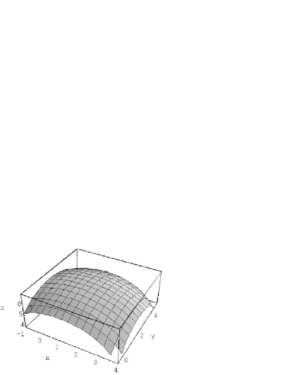
Figure 2.1: A sector of a 2-dimensional manifold embedded in Minkowski’s space-time. All points of the surface have the same proper-time $\tau=4,\tau_{0}=3,t=5,t_{0}=1,x_{0}/c=1,y_{0}/c=2$ and $z_{0}/c=3$. Obviously all events on the surface correspond to the same Newtonian time.

It is seen from this very expression for the proper-time that the same proper-time $\tau$ corresponds to all space-time points $(t,x,y,z)$ of the manifold (Figs. 2.1, 2.2), defined by

$$\tau=\sqrt{(t-t_{0})^{2}-((x-x_{0})^{2}-(y-y_{0})^{2}-(z-z_{0})^{2})/2}=\mbox{const}.$$

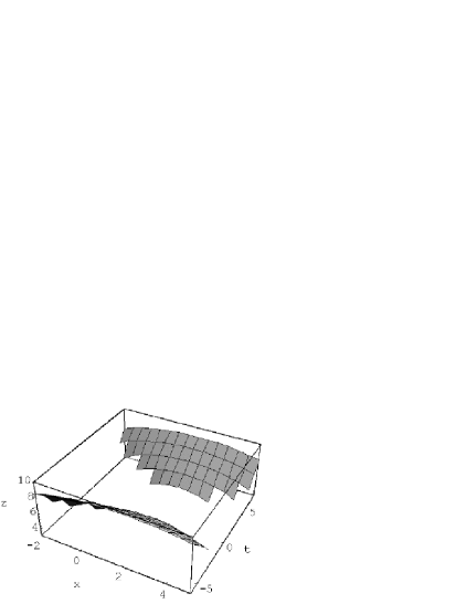
Figure 2.2: Two sectors of a 2-dimensional manifold embedded in Minkowski’s space-time having the same proper-time $\tau=4$. Here the variables are $x,z,t\cdot y=2$, while the constants are $\tau_{0}=3,t_{0}=1,x_{0}/c=2,y_{0}/c=1,z_{0}/c=3$. All events of the two sectors correspond to the same proper time, $\tau$, and $y$ values.

The source of the Einsteinian time in special relativity is the classical equation of uniform motion [45]

$$s=vt\quad\mbox{or}\quad c^{2}t^{2}-x^{2}-y^{2}-z^{2}=0,\;(m_{0}^{2}=0),$$ (2.1)

where $c$ is the velocity of light. Einstein in writing down the above equation giving the propagation distance, $s$, of a light wave front has nothing stated about the magnitude of $s$, or the length of the time interval, $[0,t]$.

The minimum operationally measurable time in connection with the light wave propagation is the time corresponding to the distance of one wave length, $\lambda$. This time, $\tau$, is related to the wave length by $\tau=\lambda/c=1/f$, where $f$ is the wave frequency. The time $\tau$ stands in a simple relation with the interaction duration causing the energy change, $\Delta E$, and with the emission of a corresponding photon. More generally, the de Broglie wave length of an emitted particle, e.g., of an electron in $\beta$-decay is related to the energy released during the emission interaction.

For the $\beta$-particle of rest mass, $m_{0}$ , which, of course, does not move on the light cone, there holds

$$c^{2}t^{2}-x^{2}-y^{2}-z^{2}=s^{\prime 2}>0\;\mbox{or}\;c^{2}-v^{2}=s>0,\;s=s^{\prime}/t.$$ (2.2)

Multiplying both sides by $c^{2}\gamma^{2}m_{0}^{2}$, where $v$ is the velocity of a quantum, one gets

$$c^{4}\gamma^{2}m_{0}^{2}=\gamma^{2}v^{2}c^{2}m_{0}^{2}+c^{2}\gamma^{2}s^{2}m_{0}^{2}.$$ (2.3)

The term on the lhs represents the total energy of the particle, whilst the first term on the rhs is equal to $c^{2}p^{2}$ . By introducing the definitions of $\gamma=(1-\beta^{2})^{-1/2},\beta=v/c$ and of $s$ the energy-momentum relation emerges,

$$E^{2}=c^{2}p^{2}+c^{4}m_{0}^{2}.$$ (2.4)

This may be considered as a clear indication that a quntization of the general rela- tivity might be obtained by formulating the field equations inside an IPN, $\tau$ , [48].

Also, it is important to notice thereby that $\tau\mathrel{\mathchoice{\raise 0.86108pt\hbox{$\scriptstyle\in$}}{\raise 0.86108pt\hbox{$\scriptstyle\in$}}{\raise 0.86108pt\hbox{$\scriptscriptstyle\in$}}{\raise 0.86108pt\hbox{$\scriptscriptstyle\in$}}}T\subset\mathchoice{\displaystyle{I\mkern-6.0muR}}{\textstyle{I\mkern-6.0muR}}{\scriptstyle{I\mkern-6.0muR}}{\scriptscriptstyle{I\mkern-6.0muR}}^{1}$. In other words the relativity time, $t$, in Minkowski space (as the Cartesian product, $M^{4}=i\mathchoice{\displaystyle{I\mkern-6.0muR}}{\textstyle{I\mkern-6.0muR}}{\scriptstyle{I\mkern-6.0muR}}{\scriptscriptstyle{I\mkern-6.0muR}}^{1}\times\mathchoice{\displaystyle{I\mkern-6.0muR}}{\textstyle{I\mkern-6.0muR}}{\scriptstyle{I\mkern-6.0muR}}{\scriptscriptstyle{I\mkern-6.0muR}}^{3}$ of the Euclidean space, $\mathchoice{\displaystyle{I\mkern-6.0muR}}{\textstyle{I\mkern-6.0muR}}{\scriptstyle{I\mkern-6.0muR}}{\scriptscriptstyle{I\mkern-6.0muR}}^{1}$ and $i\mathchoice{\displaystyle{I\mkern-6.0muR}}{\textstyle{I\mkern-6.0muR}}{\scriptstyle{I\mkern-6.0muR}}{\scriptscriptstyle{I\mkern-6.0muR}}^{3}$ ) is homeomorphic to the Newtonian time ($t\mathrel{\mathchoice{\raise 0.86108pt\hbox{$\scriptstyle\in$}}{\raise 0.86108pt\hbox{$\scriptstyle\in$}}{\raise 0.86108pt\hbox{$\scriptscriptstyle\in$}}{\raise 0.86108pt\hbox{$\scriptscriptstyle\in$}}}\mathchoice{\displaystyle{I\mkern-6.0muR}}{\textstyle{I\mkern-6.0muR}}{\scriptstyle{I\mkern-6.0muR}}{\scriptscriptstyle{I\mkern-6.0muR}}^{1}$ ).

We shall abandon the view that time, $t$, in relativity during every fundamental interaction takes values from the whole $\mathchoice{\displaystyle{I\mkern-6.0muR}}{\textstyle{I\mkern-6.0muR}}{\scriptstyle{I\mkern-6.0muR}}{\scriptscriptstyle{I\mkern-6.0muR}}^{1}$. Instead, it will be assumed throughout that $t\mathrel{\mathchoice{\raise 0.86108pt\hbox{$\scriptstyle\in$}}{\raise 0.86108pt\hbox{$\scriptstyle\in$}}{\raise 0.86108pt\hbox{$\scriptscriptstyle\in$}}{\raise 0.86108pt\hbox{$\scriptscriptstyle\in$}}}\tau$.

2.4 The Wheeler’s foam space-time topology

An interesting space-time topolology was proposed by Wheeler [14] in the framework of the geometrodynamics, a name coined by Einstein. Wheeler followed Einstein’s vision according to which all quantum phenomena - waves and particles - should be traced back to geometrical properties of a superspace-time. This superspace-time is multiply connected and its topology varies as a consequence of geometrical dynamical quantum fluctuations. The space-time structure envisaged by Wheeler very much resemles the topology of our superspace-time, but there are many substantial differences. These differences originate from both, the way of generating the superspace-time and the constants characterizing its structure.

Since Wheeler does not give a formal characterization of the topology in terms of its topological properties, we give in Table 2.1 the main properties extracted from [14] in comparison with the corresponding properties of our superspace-time.

Table 2.1: Properties of two superspace-times.

n	Property	Wheeler superspace-time	Present work
1	Origin	Quantum	Fundamental
		fluctuations	interactions
2	Symbolic	–	$({\cal T}^{\kappa 1}_{4}\oplus{\cal T}^{\kappa 2}_{4}\oplus\ldots{\cal T}^{\kappa\Lambda}_{4})\times R^{3}$
	definition
3	Geometry	Neither unique nor	Every sub-sheet is
		classical. It fluctuates	is a sub-manifold of
		everywhere with	Minkowski’s or of
		amplitudes comparable	Riemann’s space-
		to Planck’s length between	time. It is a mul-
		configurations of various	tiply disconnected
		sub-microscopic	geometry.
		curvatures and different	$\tau_{\kappa\lambda}\times R^{3}\subset\bar{M}^{4}_{\kappa\lambda}$.
		topologies.
4	Topological	The geometries which	Multiply disconnected,
		appear with high pro-	locally Hausdorff.
		babilities are multi-
		ply connected Haus-
		dorff geometries
		(foam structure).
5	Dimensions	$\quad\quad\infty^{\infty^{3}}$	$\infty^{3K}\;\forall K\mathrel{\mathchoice{\raise 0.86108pt\hbox{$\scriptstyle\in$}}{\raise 0.86108pt\hbox{$\scriptstyle\in$}}{\raise 0.86108pt\hbox{$\scriptscriptstyle\in$}}{\raise 0.86108pt\hbox{$\scriptscriptstyle\in$}}}\mathchoice{{\sevenrm Z}\mkern-9.2mu{\sevenrm Z}}{{\sevenrm Z}\mkern-9.2mu{\sevenrm Z}}{{\sevenrm Z}\mkern-9.2mu{\sevenrm Z}}{{\sevenrm Z}\mkern-9.2mu{\sevenrm Z}}^{+}$
6	Time topology	Newtonian	$\quad\quad{\cal T}_{4}$

2.5 The stochastically branching space-time model

Interesting from the point of view of the present work is the model of the stochastically branching space-time discussed by Douglas [19]. This model of space-time is inspired by the Many-World interpretation of quantum mechanics [50].

The main features of this time topological space $({\cal Y},t)\subset\mathchoice{\displaystyle{I\mkern-6.0muR}}{\textstyle{I\mkern-6.0muR}}{\scriptstyle{I\mkern-6.0muR}}{\scriptscriptstyle{I\mkern-6.0muR}}^{2}$ are: The space-time is constructed as the Cartesian product of certain open or semi-open time intervals $W_{i}(\alpha,\beta),\;i=1,2,\ldots,5$, where $(\alpha,\beta)$ are real,and $\mathchoice{\displaystyle{I\mkern-6.0muR}}{\textstyle{I\mkern-6.0muR}}{\scriptstyle{I\mkern-6.0muR}}{\scriptscriptstyle{I\mkern-6.0muR}}^{3}$ is the Euclidean space. The sets $W_{i}$ are defined by:

$$W_{1}(\alpha,\beta) = \{(t,0)\mid\alpha<t<\beta\leq 0\}$$

$$W_{2}(\alpha,\beta) = \{(t,1)\mid 0\leq\alpha<t<\beta\}$$

$$W_{3}(\alpha,\beta) = \{(,0)\mid\alpha<t<0\}\cup\{(t,1)\mid 0\leq t<<\beta\}$$

$$W_{4}(\alpha,\beta) = \{(t,-1)\mid 0\leq\alpha<t<\beta\}$$

$$W_{5}(\alpha,\beta) = \{(t,0)\mid\alpha<t<0\}\cup\{(t,-1)\mid 0\leq t<\beta\}$$

The main properties of this space-time are:

• It is locally Euclidean.

• It is not Hausdorff.

• It associates probabilistic properties with the topology of the space-time.

• It is based on the Many-World interpretation of quantum mechanics.

• The time topology cannot accommodate in general physical interactions, because they take place in the present $t=0$ of the rest frame of reference. This point in the model is not uniquely defined.

The above given sets have topological cuts at $t=0$. more precisely: $W_{1}(\alpha,\beta)$ represents the lower section of the time (past) and it has no largest element. $W_{2}(\alpha,\beta)$ and $W_{4}(\alpha,\beta)$ represent the upper sections (futures) and they have no smallest elements. $W_{3}(\alpha,\beta)$ and $W_{5}(\alpha,\beta)$ consist of two lower sections and two upper sections. The lower sections have no largest and the upper sections have smallest elements.

This time topological space $({\cal Y},\tau)$ has the structure in the simplest case

$${\cal Y}=\{(t,0)\mid t<0\}\cup\{(t,1)\mid t\geq 0\}\cup\{(t,-1)\mid t\geq 0\}\subset\mathchoice{\displaystyle{I\mkern-6.0muR}}{\textstyle{I\mkern-6.0muR}}{\scriptstyle{I\mkern-6.0muR}}{\scriptscriptstyle{I\mkern-6.0muR}}^{2}.$$ (2.5)

It is seen from the above that the ’present’, which is the only directly observable part of the time consists, of a cut in $\mathchoice{\displaystyle{I\mkern-6.0muR}}{\textstyle{I\mkern-6.0muR}}{\scriptstyle{I\mkern-6.0muR}}{\scriptscriptstyle{I\mkern-6.0muR}}^{1}$, because the past of the model has no largest element, and the future has a least element $(t=0)$. This topological structure of the ’present’ makes ambiguous the solution of the fundamental time-dependent differential equations of physics at $t=0$ describing transitions from $t<0$ to $t>0$ (Fig. 2.3 ).

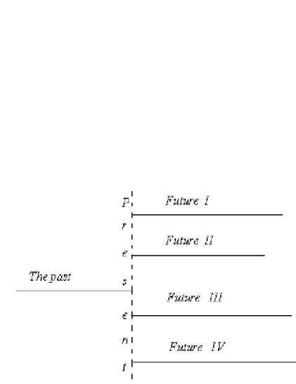
Figure 2.3: The simplest case of Douglas’ time-topological space. The fundamental time-dependent differential equations of physics (Schroedinger, Dirac, quantum field theories) are not unique at the ’present, $t=0$. The time line has a cut at $t=0$, and is for $t=0+\epsilon$ multivalued.

It should be pointed out that all experimental physical measuring processes take place at the ’present’ of any time topology. Just this point is not uniquely defined in Douglas time topology. On the other hand, of course, measurements in the past time or in future states of a given quantum system are, in general, impossible.

The existence of the cut implies that between any particular open set $\{(0,t)\mid t\leq-0\}$ and the present, $t=0$, of the open sets $\{(t,n)\mid t\geq 0,n=\pm 1,\pm 2,\ldots\}$ there must exist neighbourhoods of time points which do not contain the ’present’ $t=0$ for particles coming from the past.

Also, the transition from the ’past’ to the ’present’, at which a future state is generated, happens during a time interval of measure equal to zero. This is not in agreement with the experimental evidence according to which interactions are associated with a finite duration.

3 Chrono-topology and space-time of the fundamental quantum interactions

We mentioned in various occasions in the foregoing sections the reasons for which the Newtonian universal time must be replaced by the appropriate time-space topology. We are going to discuss in this section more in depth the time problem and its consequences for the quantum processes resulting from the $\mathchoice{\displaystyle{I\mkern-6.0muR}}{\textstyle{I\mkern-6.0muR}}{\scriptstyle{I\mkern-6.0muR}}{\scriptscriptstyle{I\mkern-6.0muR}}^{1}$ topology assumes in the past.

3.1 Operational meaning of the commutation relations

The idea that time is related to energy changes is not new. Already Schroedinger and Pauli considered the relation of the time with the energy as a direct consequence of the commutation relations

$$[x,p]=i\hbar I\delta_{\mu\nu}\>\mu,\nu=1,2,3.$$ (3.1)

However, the position coordinate, $x$, and the conjugate momentum, $p_{x}$, are related, despite their independence in the sense of the mathematical analysis of the phase space mechanics, not just by the commutation relations. There is still an other reciprocal physical relationship: The change, $\Delta x$, of the position variable, $x$, of a particle generates its momentum, $p_{x}$. The converse is also true. The change of the momentum, $p_{x}$, (or even its mere existence) of a particle necessarily implies change, $\Delta x$, of its position, $x$. This mutual relationship has not been sufficiently emphasized although its existence is quite evident. This relationship will prove very instructive in the following considerations about the generation of time.

The commutation relation between the energy operator $H$ and the time operator $t$ is [51]-[52]

$$[t,H]=i\hbar I.$$ (3.2)

The ”generating” relationship between energy change and time change is apparent here, as it was in (3.1), for the pair $(x,p_{x})$.

In quite a similar way, the change, $\Delta E$, of the energy of a particle generates the time laps, $\Delta t$, which is appropriate for the description of this particular event [1].

A further analogy between (3.1) and (3.2) of great importance for the understanding of the nature of the time is the following: The result of applying (3.1) on a wave function is to describe the creation of a quantum pertaining to the particle having the momentum, $p_{x}$.

Similarly, the application of (3.2) on a wave function creates a quantum pertaining to the particle having the energy $E$.

It is appropriate to emphasize that every time neighbourhood pertains to the particle in its rest frame subject to the corresponding interaction. It would not be in agreement with relativity, if the same time neighbourhood would be used universally to describe the evolution of other interactions at different points of the space.

3.2 Change and time

By ”mixing” the time and the space variables, as it happens in the Lorentz transformation, we do not yet fully eliminate the classical, absolute character of the time. Such should be achieved better by attaching to every one act of elementary energy changing interaction its own time neighbourhood. It takes values exactly as long as the interaction is going on.

Considering that in a many particle system each particle’s history is described by its own set of time neighbourhoods - each one starting and ending with the starting and the ending of the corresponding interaction (causing associated changes in observables of the respective particle) - it is not obvious at first sight, which one of the many ”pieces” of time (which, by the way, clearly may overlap partially or entirely, in the sense of the relativistic simultaneity) would be appropriate to descricribe the set of particles as a physical system. This difficulty is avoided by introducing the notion of the IPN. In conformity with the above ideas we shall prove the following

Proposition 3.1

The changes $(\Delta x^{\prime},\Delta t^{\prime})$ of the coordinates $(x^{\prime},t^{\prime})$ in observer’s moving reference system of an event $(x,t)$ in its rest system of reference are linear functions of the changes $(\Delta x,\Delta t)$.

Proof

Consider the Lorentz transformations:

$$x^{\prime}=\gamma(x-vt)$$ (3.3)

and

$$t^{\prime}=\gamma(t-(\beta/c)x).$$ (3.4)

where $\gamma=1/\sqrt{(1-\beta^{2})},\beta=v/c.$

Let $x=0$ in (3.3). Any change $\Delta t$, of the time $t$, is a linear function of the change $\Delta x$ of $x$. The converse is also true: It follows from (3.4) that the change $\Delta t^{\prime}$, of the time $t^{\prime}$, for $t=0$ is a linear function of the change, $\Delta x$, of the space variable, $x$, and vice versa.

Therefore:

$$\Delta x^{\prime}=-\gamma v\Delta t,$$ (3.5)

$$\Delta t^{\prime}=-\gamma(\beta/c)x$$ (3.6)

and the proof is complete.

Remark 3.1

This obvious and rather trivial result is known to many people since almost one century. However, its special meaning seems to have escaped hitherto our attention: If we convene to consider the coordinate $x$ as an observable, then (3.6) is a regular, continuous map of the change of an observable to a linear set, the IPN.

Table 3.1: Orders of magnitude of the IPNs for QED and QCD following from (3.5), (3.6) and the magnitudes of atoms and nuclei.

Theory	$\beta$	approx. radius $[m]$	IPN diameter $\delta(\tau)\>[s]$
QED	.1	$10^{-10}$	$10^{-19}$
QCD	.1	$10^{-15}$	$10^{-24}$

In addition, $\Delta x$ represents in physics the displacement of, e.g., a particle. By generalizing this to any observable change one obtains a map of the changes onto the time-space. This is a generalization of Proposition 3.1.

3.3 The construction of the time-space topology

The following Definition 3.1 and Definition 3.2 are considered as the two axioms of the present new chrono-topology developed in this work.

Axiom I.

All time definitions, classical or quantal, are based on some process implementing a change, natural or technical and generates time neighbourhoods. The generated IPN’s are regular, into-maps of just these changes.

Axiom II.

Every fundamental interaction is associated with (different among them, but) finite changes of the involved physical observables. The changes of the observables have intrinsic the random character, as to their embedment in the Newtonian time. They start at irregular Newtonian times and have, within limits, stochastically distributed durations. They may be thought of as embedded in the Newtonian universal time, $\mathchoice{\displaystyle{I\mkern-6.0muR}}{\textstyle{I\mkern-6.0muR}}{\scriptstyle{I\mkern-6.0muR}}{\scriptscriptstyle{I\mkern-6.0muR}}^{1}$, but their union has not the topology $\mathchoice{\displaystyle{I\mkern-6.0muR}}{\textstyle{I\mkern-6.0muR}}{\scriptstyle{I\mkern-6.0muR}}{\scriptscriptstyle{I\mkern-6.0muR}}^{1}$.

Axiom III.

The elements of an empty set, $\emptyset$, of a class of observable sets $\{O_{\lambda}|\lambda\mathrel{\mathchoice{\raise 0.86108pt\hbox{$\scriptstyle\in$}}{\raise 0.86108pt\hbox{$\scriptstyle\in$}}{\raise 0.86108pt\hbox{$\scriptscriptstyle\in$}}{\raise 0.86108pt\hbox{$\scriptscriptstyle\in$}}}Z^{+}\}$ are not observable, and their values are identically equal to zero.

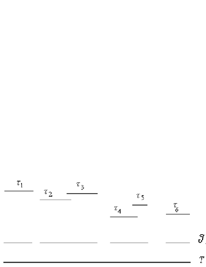
Figure 3.1: Representation of six IPNs $\{\tau_{i}|i=1,2,\ldots 6\}$, the union, ${\cal T}_{4}$, of their projections, and a subset, $T\subset\mathchoice{\displaystyle{I\mkern-6.0muR}}{\textstyle{I\mkern-6.0muR}}{\scriptstyle{I\mkern-6.0muR}}{\scriptscriptstyle{I\mkern-6.0muR}}^{1}$, of the Newtonian universal time, $\mathchoice{\displaystyle{I\mkern-6.0muR}}{\textstyle{I\mkern-6.0muR}}{\scriptstyle{I\mkern-6.0muR}}{\scriptscriptstyle{I\mkern-6.0muR}}^{1}$, in which ${\cal T}_{4}$ may be considered as embedded.

Here is the principal definition of the interaction proper-time neighbourhood, the IPN:

Definition 3.1

Let $O$ be an observable characterizing one or both of a given pair of interacting quanta. Let $\Delta O$ be the corresponding change due to a fundamental interaction. We define the IPN (interaction proper-time neighbourhood) as the regular and continuous map:

$$\tau_{\lambda}=IPN=f:\Delta O\rightarrow\tau_{\lambda}=f(\Delta O)\mathrel{\mathchoice{\raise 0.86108pt\hbox{$\scriptstyle\in$}}{\raise 0.86108pt\hbox{$\scriptstyle\in$}}{\raise 0.86108pt\hbox{$\scriptscriptstyle\in$}}{\raise 0.86108pt\hbox{$\scriptscriptstyle\in$}}}{\cal T}_{4}.$$ (3.7)

IPN is the time ”quantum” of the process corresponding to the fundamental interaction under consideration, characteristic of and proper to that interaction and only to that.

3.4 The many-folded super space-time

Definition 3.2

1. Let $K\times\Lambda_{K}$ pairs of quanta interact.

2. Let $\{T_{K}|\>\kappa\mathrel{\mathchoice{\raise 0.86108pt\hbox{$\scriptstyle\in$}}{\raise 0.86108pt\hbox{$\scriptstyle\in$}}{\raise 0.86108pt\hbox{$\scriptscriptstyle\in$}}{\raise 0.86108pt\hbox{$\scriptscriptstyle\in$}}}[1,K]\equiv I_{K}\subset\mathchoice{{\sevenrm Z}\mkern-9.2mu{\sevenrm Z}}{{\sevenrm Z}\mkern-9.2mu{\sevenrm Z}}{{\sevenrm Z}\mkern-9.2mu{\sevenrm Z}}{{\sevenrm Z}\mkern-9.2mu{\sevenrm Z}}^{+}\}$ be a family of subsets $T_{K}\subset\mathchoice{\displaystyle{I\mkern-6.0muR}}{\textstyle{I\mkern-6.0muR}}{\scriptstyle{I\mkern-6.0muR}}{\scriptscriptstyle{I\mkern-6.0muR}}^{1}$ such that $\{T_{K}\cap T_{K^{\prime}}=\emptyset\>|\>\forall(\kappa,\kappa^{\prime}]\mathrel{\mathchoice{\raise 0.86108pt\hbox{$\scriptstyle\in$}}{\raise 0.86108pt\hbox{$\scriptstyle\in$}}{\raise 0.86108pt\hbox{$\scriptscriptstyle\in$}}{\raise 0.86108pt\hbox{$\scriptscriptstyle\in$}}}I_{K}\subset\mathchoice{{\sevenrm Z}\mkern-9.2mu{\sevenrm Z}}{{\sevenrm Z}\mkern-9.2mu{\sevenrm Z}}{{\sevenrm Z}\mkern-9.2mu{\sevenrm Z}}{{\sevenrm Z}\mkern-9.2mu{\sevenrm Z}}^{+}\}.$

3. Let $\{\tau_{\kappa\lambda_{\kappa}}\mathrel{\mathchoice{\raise 0.86108pt\hbox{$\scriptstyle\in$}}{\raise 0.86108pt\hbox{$\scriptstyle\in$}}{\raise 0.86108pt\hbox{$\scriptscriptstyle\in$}}{\raise 0.86108pt\hbox{$\scriptscriptstyle\in$}}}T_{K},\>\forall\lambda_{\kappa}\mathrel{\mathchoice{\raise 0.86108pt\hbox{$\scriptstyle\in$}}{\raise 0.86108pt\hbox{$\scriptstyle\in$}}{\raise 0.86108pt\hbox{$\scriptscriptstyle\in$}}{\raise 0.86108pt\hbox{$\scriptscriptstyle\in$}}}[1,\Lambda_{K}]\equiv I_{\Lambda_{K}}\}$ be a family of IPNs such that

   $$\{\tau_{\kappa\lambda_{\kappa}}\cap\tau_{\kappa\lambda_{\kappa}^{\prime}}=\emptyset\mbox{ for}\>\lambda_{\kappa}\neq\lambda_{\kappa}^{\prime}\}.$$

We define:

1. The $\Lambda_{\kappa}$-fold, disconnected time-space by

   $${\cal T}^{(\Lambda\kappa)}_{4}=\tau_{\kappa 1}\oplus\tau_{\kappa 2}\oplus\ldots\oplus\tau_{\kappa\Lambda_{\kappa}}.$$ (3.8)

   $\{\delta(\tau_{\kappa\lambda_{\kappa}})\}$ may be thought as the random absolute values of vectors orthogonal at every point of Riemann space-like super-surfaces.

2. The $\Lambda_{\kappa}$-fold, disconnected super-space-time in the sense of $\lambda_{\kappa}$-fold Riemann super-space-time by

   $$\bar{M}^{4}_{\Lambda_{\kappa}}=i\left(\tau_{1}\oplus\tau_{2}\oplus\ldots\oplus\tau_{\Lambda_{\kappa}}\right)\times\mathchoice{\displaystyle{I\mkern-6.0muR}}{\textstyle{I\mkern-6.0muR}}{\scriptstyle{I\mkern-6.0muR}}{\scriptscriptstyle{I\mkern-6.0muR}}^{3},$$ (3.9)

   where $\mathchoice{\displaystyle{I\mkern-6.0muR}}{\textstyle{I\mkern-6.0muR}}{\scriptstyle{I\mkern-6.0muR}}{\scriptscriptstyle{I\mkern-6.0muR}}^{3}$ is a 3-dimensional Riemann space.

The formulation of a physical theory in terms of generalized random and infinitely divisible fields requires space-time structures of the above form.

To make this clear, let us consider one single IPN, $\tau_{1}$, and the corresponding space-time, $\bar{M}^{4}_{\kappa 1}$. The lower index signifies that $\bar{M}^{4}_{\kappa 1}=i\tau_{\kappa 1}\times\mathchoice{\displaystyle{I\mkern-6.0muR}}{\textstyle{I\mkern-6.0muR}}{\scriptstyle{I\mkern-6.0muR}}{\scriptscriptstyle{I\mkern-6.0muR}}^{3}$, and this space-time is simple in time, i.e., a subset of a Riemann space. If $\mathchoice{\displaystyle{I\mkern-6.0muR}}{\textstyle{I\mkern-6.0muR}}{\scriptstyle{I\mkern-6.0muR}}{\scriptscriptstyle{I\mkern-6.0muR}}^{3}$ is flat, then $\bar{M}^{4}_{\kappa 1}$ becomes a subset of the Minkowski space.

If there are two different IPNs, ${(\tau_{\kappa 1},\tau_{\kappa 2})}$ such that on the one hand $\tau_{\kappa 1}\cap\tau_{\kappa 2}=\emptyset$ and on the other hand their projections $\pi_{1},\pi_{2}$ into $T_{\kappa}$ satisfy $\pi_{1}\subseteq\pi_{2}$, then the corresponding space-time is $\bar{M}^{4}_{2}=i(\tau_{\kappa 1}\oplus\tau_{\kappa 2})\times\mathchoice{\displaystyle{I\mkern-6.0muR}}{\textstyle{I\mkern-6.0muR}}{\scriptstyle{I\mkern-6.0muR}}{\scriptscriptstyle{I\mkern-6.0muR}}^{3}$. This space-time is two-fold in time. In case $\mathchoice{\displaystyle{I\mkern-6.0muR}}{\textstyle{I\mkern-6.0muR}}{\scriptstyle{I\mkern-6.0muR}}{\scriptscriptstyle{I\mkern-6.0muR}}^{3}=E^{3}$, the Euklidian $3$-space, $\bar{M}^{4}_{2}$ is not a subset of Minkowski’s space anymore.

It is said in terms of relativistic simultaneity fully or partly simultaneous according to the relations

$$(\pi_{1}\subseteq\pi_{2})\wedge(\pi_{1}\supseteq\pi_{2})\quad\mbox{or}\quad(\pi_{1}\subseteq\pi_{2})\vee\pi_{2}\subseteq\pi_{1})$$

respectively.

More generally, if $\lambda_{\kappa}$ IPNs satisfy

$$\tau_{\kappa\lambda_{\kappa}}\cap\tau_{\kappa\lambda_{\kappa}^{\prime}}=\emptyset,\quad\forall(\lambda_{\kappa},\lambda_{\kappa}^{\prime})\mathrel{\mathchoice{\raise 0.86108pt\hbox{$\scriptstyle\in$}}{\raise 0.86108pt\hbox{$\scriptstyle\in$}}{\raise 0.86108pt\hbox{$\scriptscriptstyle\in$}}{\raise 0.86108pt\hbox{$\scriptscriptstyle\in$}}}I_{\kappa}$$

and their projections into $T_{\kappa}$

$$(\pi_{\lambda_{\kappa}}\subseteq\pi_{\lambda_{\kappa}^{\prime}})\wedge(\pi_{\lambda_{\kappa}}\supseteq\pi_{\lambda_{\kappa}^{\prime}})\quad\mbox{or}\quad(\pi_{\lambda_{\kappa}}\subseteq\pi_{\lambda_{\kappa}^{\prime}})\vee(\pi_{\lambda_{\kappa}^{\prime}}\subseteq\pi_{\lambda_{\kappa}}),\quad\forall(\lambda_{\kappa},\lambda_{\kappa}^{\prime})\mathrel{\mathchoice{\raise 0.86108pt\hbox{$\scriptstyle\in$}}{\raise 0.86108pt\hbox{$\scriptstyle\in$}}{\raise 0.86108pt\hbox{$\scriptscriptstyle\in$}}{\raise 0.86108pt\hbox{$\scriptscriptstyle\in$}}}I_{\kappa},$$

then the strucure of $\bar{M}^{4}_{\kappa\lambda_{\kappa}}$ is even higher.

In a $\lambda_{\kappa}$-fold in time space-time the decomposition of a divisible field $\cal L$ in up to ${\lambda_{\kappa}}$ terms is possible without interfering neither with the definition of the function notion nor with the conservation laws of physics cases in which $f(x)\neq 2f(x)$. An illustration of our time-space $K=4,(\Lambda_{1}=1,\Lambda_{2}=2,\Lambda_{3}=2,\Lambda_{4}=1)$, is given in Fig 3.1, while the case $K=3,(\Lambda_{1}=2,\Lambda_{2}=3,\Lambda_{3}=\kappa)$ time-space is shown in Fig. 3.2 .

Figure 3.2: Three types of many-folded time topological time-spaces, two-fold, ${\cal T}^{2}_{4}$, three-fold, ${\cal T}^{3}_{4}$ and $\kappa$-fold, ${\cal T}^{\kappa}_{4}$. These time-spaces give rise to the creation of the space-times, $\bar{M}^{4}_{12},\bar{M}^{4}_{23},\bar{M}^{4}_{3\kappa}$.

It is important that the time in, e.g., the rest frame of a particle is related to its corresponding interaction. If to all IPNs were given the properties of one single IPN, the time-space would lose its randomness.

We put just this time in the equations of Schroedinger, of Dirac and of QFT in connection with problems of nuclear and sub-nuclear intereactions. The time change within an IPN cannot generate the impression of flowing: i) it escapes the discrimination power of the human sensors, and ii) There is one single IPN and no ordering is feasible.

On the contrary, for a moving observer the reaction time may flow or not flow further depending, according to (3.4) above, on whether the particle changes either its position, $x$, or its time, $t$, or both, or any other of its observables. Hence, it is clear that the particle reaction time cannot be identified with the universal time which is the union of the maps of all observable changes, occurring in the entire observable universe.

Remark 3.2

The factor ${\cal T}_{4}$ determines the structure of the new space-time $\bar{M}^{4}_{\kappa}$.

The space-time, $\bar{M}^{4}_{\kappa\lambda_{\kappa}}$, $\lambda_{\kappa}$-fold in time is the natural space-time for the application of the theory of the generalized and inifinitely divisible fields.

Remark 3.3

Time-dependent quantum equations not including interactions do not supply us with any physical information regarding the evolution of the particle system. For example, an electron moving in vacuum without interaction is described by free-field quantum time-dependent equations, but it does not exist, it is not observable.

However, the situation is still more complex: The kind of time topology Nature chooses in every individual case of interacting particle systems, depends on the number of the interacting particle pairs and on whether the interactions are partially or totally simultaneous in the sense of relativity. One easily realizes based on our definition of the time that the topological space, ${\cal T}_{4}$, tends to the space with the natural topolgy of $\mathchoice{\displaystyle{I\mkern-6.0muR}}{\textstyle{I\mkern-6.0muR}}{\scriptstyle{I\mkern-6.0muR}}{\scriptscriptstyle{I\mkern-6.0muR}}^{1}$, if the number of the interacting particles becomes very large and the intersections of the adjacent IPNs are not empty anymore [48]. More precisely:

$$\{({\cal T}_{4}=\mbox{\it natural topology of }T_{\Lambda}\rightarrow\mathchoice{\displaystyle{I\mkern-6.0muR}}{\textstyle{I\mkern-6.0muR}}{\scriptstyle{I\mkern-6.0muR}}{\scriptscriptstyle{I\mkern-6.0muR}}^{1})\wedge(\bar{M}^{4}_{\Lambda}\rightarrow M^{4})\mbox{ for }\Lambda\rightarrow\mathchoice{{\sevenrm Z}\mkern-9.2mu{\sevenrm Z}}{{\sevenrm Z}\mkern-9.2mu{\sevenrm Z}}{{\sevenrm Z}\mkern-9.2mu{\sevenrm Z}}{{\sevenrm Z}\mkern-9.2mu{\sevenrm Z}}^{+}\}$$ (3.10)

$\bar{M}^{4}_{\Lambda}$ is the physical space-time created by the dynamics and yields the scenery for the evolution of the dynamical particle systems.

$M^{4}$, Minkowki’s space-time, is a mathematical object representing the limit of $\bar{M}^{4}_{\Lambda}$ for an infinity of interacting particles, such that $\{\tau_{\lambda}|\>\forall\lambda\mathrel{\mathchoice{\raise 0.86108pt\hbox{$\scriptstyle\in$}}{\raise 0.86108pt\hbox{$\scriptstyle\in$}}{\raise 0.86108pt\hbox{$\scriptscriptstyle\in$}}{\raise 0.86108pt\hbox{$\scriptscriptstyle\in$}}}\Lambda\rightarrow\mathchoice{{\sevenrm Z}\mkern-9.2mu{\sevenrm Z}}{{\sevenrm Z}\mkern-9.2mu{\sevenrm Z}}{{\sevenrm Z}\mkern-9.2mu{\sevenrm Z}}{{\sevenrm Z}\mkern-9.2mu{\sevenrm Z}}^{+}\}$ is a covering basis of $\mathchoice{\displaystyle{I\mkern-6.0muR}}{\textstyle{I\mkern-6.0muR}}{\scriptstyle{I\mkern-6.0muR}}{\scriptscriptstyle{I\mkern-6.0muR}}^{1}$.

3.5 Randomness and covariance

The randomness of the IPNs in a set of interacting particles is a direct consequence of the randomness of the interaction durations. Also the randomness of the physical fields as well as the resolution of some paradoxes in quantum theory can be understood on the basis of the topology of ${\cal T}_{4}$ in the rest frame of the interacting particles.

1. The topology of the time-space in the reference frame of a moving observer is determined through Lorentz transforming the time-space ${\cal T}_{4}$ to the time of moving observers with respect to interacting particles.

2. All functions $f(x)$ of the space-time coordinates $(x^{0},x^{1},x^{2},x^{3})\mathrel{\mathchoice{\raise 0.86108pt\hbox{$\scriptstyle\in$}}{\raise 0.86108pt\hbox{$\scriptstyle\in$}}{\raise 0.86108pt\hbox{$\scriptscriptstyle\in$}}{\raise 0.86108pt\hbox{$\scriptscriptstyle\in$}}}\bar{M}^{4}_{\kappa}$ bear the random character of the time topology of ${\cal T}_{4}$.

3. In the topology of space-times resulting from ${\cal T}_{4}$ the time and the space do not flow. The domain of the coordinates $\{x^{\mu}|\mu=0,1,2,3\}$ is compact in the subsets of the disconnected space-time $\bar{M}^{4}_{\kappa}$.

The above observations give rise to the question as to the covariance of the fundamental equations of QFT in the super space-time. It is not difficult to see that this aspect of the theory does not suffer any important change.

Since every single physical process takes place inside its respective IPN, it is sufficient to verify that the equations of quantum mechanics and of QFT remain covariant for the Poincare transformation group within the space-time for $\bar{M}^{4}_{\kappa}$ for $\kappa=1$. The Noether theorem is valid in every IPN and the proof is identical to the usual proof in the Minkowski space-time and it is omitted.

3.6 Chrono-topology and irreversibility considerations

The chrono-topology opens new possibilities for the investigation of the $\bf U$ and $\bf R$ kinds of time evolution. We continue here the the examination of these aspects.

• The fundamental equations of physics - including interactions - as well as the phenomena described by them are time-reversal invariant on every single IPN, $\tau$. The conservation laws are valid for $\bf U$ processes. All phenomena are time reversible inside one and the same IPN, $\tau$, during $\bf U$ time evolution.

• But (attention!) the event that the time-reversed interaction action-integral equals the action-integral of the (factual) reverse interaction has a zero probability measure.

The probability measures for these processes have the following properties:

• The measure, $\mu_{Direct}$, for the direct process is associated with a mathematically realizable and physically possible process.

• The measure, $\mu_{Time-reversed}$, for the time-reversed process is associated with a mathematically realizable process wich is physically impossible.

• The measure, $\mu_{Reverse\>interaction}$, for the reverse interaction corresponds to a process both mathematically and physically possible. It is important to realize that a time reversed and a factually reverse reaction do not take place in the same $\tau$.

  The combinations of the measures have the properties:

$$\mu_{Direct},\mu_{Time-reversed},\mu_{Reverse\>interaction} > 0,$$

$$\mbox{\it Probability measure}\{\mu_{Direct}=\mu_{Reverse\>interaction}\} = 0,$$

$$\mbox{\it Probability measure}\{\mu_{Direct}=\mu_{Time-reversed}\} = 1.$$

These relations can become more clear with the help of three, generally, different well-ordered IPNs IPNs $\{\tau_{1}\succ\tau_{2}\succ\tau_{3}\}$. Suppose that the direct and the time reversed reactions take place for $t\mathrel{\mathchoice{\raise 0.86108pt\hbox{$\scriptstyle\in$}}{\raise 0.86108pt\hbox{$\scriptstyle\in$}}{\raise 0.86108pt\hbox{$\scriptscriptstyle\in$}}{\raise 0.86108pt\hbox{$\scriptscriptstyle\in$}}}\tau_{2}$. Since the factually reverse reaction cannot proceed simultaneously with the direct reaction, it will take place either in $\tau_{1}\succ\tau_{2}$ or in $\tau_{3}\prec\tau_{2}$.

$$\{\mbox{\it TIME-REVERSED action}\quad\int dtH(t),\quad t\mathrel{\mathchoice{\raise 0.86108pt\hbox{$\scriptstyle\in$}}{\raise 0.86108pt\hbox{$\scriptstyle\in$}}{\raise 0.86108pt\hbox{$\scriptscriptstyle\in$}}{\raise 0.86108pt\hbox{$\scriptscriptstyle\in$}}}\tau_{2}\}\neq$$

$$\{\mbox{\it action }\quad\int dtH(t)\quad\mbox{\it of the REVERSE interaction }\quad(t\mathrel{\mathchoice{\raise 0.86108pt\hbox{$\scriptstyle\in$}}{\raise 0.86108pt\hbox{$\scriptstyle\in$}}{\raise 0.86108pt\hbox{$\scriptscriptstyle\in$}}{\raise 0.86108pt\hbox{$\scriptscriptstyle\in$}}}\tau_{1}\succ\tau_{2})\vee(t\mathrel{\mathchoice{\raise 0.86108pt\hbox{$\scriptstyle\in$}}{\raise 0.86108pt\hbox{$\scriptstyle\in$}}{\raise 0.86108pt\hbox{$\scriptscriptstyle\in$}}{\raise 0.86108pt\hbox{$\scriptscriptstyle\in$}}}\tau_{3}\prec\tau_{2})\}.$$

The above relation (i.e., ”time-reversed process action” is different from the ”action of the factually reverse process”) holds true, because the IPNs

$$\{\tau_{1},\tau_{2},\tau_{3}\}$$

may be different in two respects:

1. As sets.

2. As set diameters, $\{\delta(\tau_{\lambda}),\lambda=1,2,3\}.$

On the other hand, the ranges of any functions in $\{\tau_{1},\tau_{2},\tau_{3}\}$ are, with high probability, different at least for two reasons:

• $\delta(\tau_{\lambda}),\lambda=1,2,3$, as numbers: Probability measure $\{\delta(\tau_{i})=\delta(\tau_{j}),j\neq i\}=0$, and

• $\tau_{\lambda},\lambda=\>1,2,3$ as point sets: Probability measure $\left\{\{\tau_{i}\}\cap\{\tau_{j}\}=\emptyset\right\}=1,j\neq i.$

3.7 Planck time and chrono-topology

Despite the differences between our space-time topology in conception and in construction method and the space-time foam of S. Hawking [24] there is, nevertheless, a certain resemblance at the limit $\delta(\tau_{\lambda})\rightarrow\mbox{\it Planck time }\>\forall\lambda\mathrel{\mathchoice{\raise 0.86108pt\hbox{$\scriptstyle\in$}}{\raise 0.86108pt\hbox{$\scriptstyle\in$}}{\raise 0.86108pt\hbox{$\scriptscriptstyle\in$}}{\raise 0.86108pt\hbox{$\scriptscriptstyle\in$}}}\mathchoice{{\sevenrm Z}\mkern-9.2mu{\sevenrm Z}}{{\sevenrm Z}\mkern-9.2mu{\sevenrm Z}}{{\sevenrm Z}\mkern-9.2mu{\sevenrm Z}}{{\sevenrm Z}\mkern-9.2mu{\sevenrm Z}}^{+}$, when the interactions become very fast.

If the ”foam” time intervals had all the Planck time magnitude they would loose the random character.

If the observers lived in $\tau$, it would be impossible to compare $\tau_{j}$ with $\tau_{i}$ for $i\neq j$, because each $\tau$ is its own unit in the rest frame. However, such a comparison is for the human observers perfectly possible, because our senses are exposed to quanta coming from many different, but, more or less, overlapping interactions in $T\subset\mathchoice{\displaystyle{I\mkern-6.0muR}}{\textstyle{I\mkern-6.0muR}}{\scriptstyle{I\mkern-6.0muR}}{\scriptscriptstyle{I\mkern-6.0muR}}^{1}$, due to our ability to observe (almost) simultaneously more than one physical changes.

The time-space topology ${\cal T}_{4}$ introduced above bears intrinsically the random character of the IPNs. It is this property that imposes randomness to every function of the time. An important observation is that the randomness can be perceived by the observers, because they are living in the background of the Newtonian time which has the topology of $\mathchoice{\displaystyle{I\mkern-6.0muR}}{\textstyle{I\mkern-6.0muR}}{\scriptstyle{I\mkern-6.0muR}}{\scriptscriptstyle{I\mkern-6.0muR}}^{1}$.

Some examples of functions defined in $\tau$ becoming random are:

• The space-time coordinates for the moving observer of a particle system. The observers are almost in all cases moving with respect to the interacting elementary particles, so that observation is mediated by Lorenz transformations.

• All observables expressed as functions of the space-time coordinates in the rest frame of reference of the observer.

• The components of the quantum fields which become generalized random fields.

• The Hamiltonian and the Lagrangian densities become generalized random and infinitely divisible fields, thus admitting the representation

  $$F(\phi(x),\partial\phi(x))=F(\phi(x_{1}),\partial\phi(x_{1}))+F(\phi(x_{2}),\partial\phi(x_{2}))+\ldots+F(\phi(x_{\lambda}),\partial\phi(x_{\lambda})),$$

  $$\kappa=2,3,\ldots\mbox{ for }x\mathrel{\mathchoice{\raise 0.86108pt\hbox{$\scriptstyle\in$}}{\raise 0.86108pt\hbox{$\scriptstyle\in$}}{\raise 0.86108pt\hbox{$\scriptscriptstyle\in$}}{\raise 0.86108pt\hbox{$\scriptscriptstyle\in$}}}\bar{M}_{\kappa}^{4}.$$

  for $\kappa\mathrel{\mathchoice{\raise 0.86108pt\hbox{$\scriptstyle\in$}}{\raise 0.86108pt\hbox{$\scriptstyle\in$}}{\raise 0.86108pt\hbox{$\scriptscriptstyle\in$}}{\raise 0.86108pt\hbox{$\scriptscriptstyle\in$}}}\mathchoice{{\sevenrm Z}\mkern-9.2mu{\sevenrm Z}}{{\sevenrm Z}\mkern-9.2mu{\sevenrm Z}}{{\sevenrm Z}\mkern-9.2mu{\sevenrm Z}}{{\sevenrm Z}\mkern-9.2mu{\sevenrm Z}}^{+}$ and with probability distributions independent of $\kappa$.

• The metric tensor $g_{\mu\nu}$ of the space-time in general relativity.

  The IPNs, as maps of finite observables’ changes through interactions, they are each one compact in $T\subset\mathchoice{\displaystyle{I\mkern-6.0muR}}{\textstyle{I\mkern-6.0muR}}{\scriptstyle{I\mkern-6.0muR}}{\scriptscriptstyle{I\mkern-6.0muR}}^{1}$, and their set diameters are empirically inversely proportional to the strength of the interaction.

4 Microscopic and macroscopic system-time

The considerations of the foregoing sections make clear that any time variable defined to describe a microscopic system will be conceived as the union of IPNs $\{\tau\}$ generated during the numerous interactions of atomic, nuclear or sub-nuclear constituents of the system under observation. It becomes, therefore, clear that every sytem of particles has its own macroscopic time given by the union in question. If two different particle system S and S’ have equal numbers N=N’ of identical particles, interacting via identical forces, they may or may not have identical microscopic IPNs.Because the changes of the observables and, consequently, their maps, the interaction proper-time neighbourhoods, are random.

If the numbers of the interactions $i,i^{\prime}\mathrel{\mathchoice{\raise 0.86108pt\hbox{$\scriptstyle\in$}}{\raise 0.86108pt\hbox{$\scriptstyle\in$}}{\raise 0.86108pt\hbox{$\scriptscriptstyle\in$}}{\raise 0.86108pt\hbox{$\scriptscriptstyle\in$}}}I\subset\mathchoice{{\sevenrm Z}\mkern-9.2mu{\sevenrm Z}}{{\sevenrm Z}\mkern-9.2mu{\sevenrm Z}}{{\sevenrm Z}\mkern-9.2mu{\sevenrm Z}}{{\sevenrm Z}\mkern-9.2mu{\sevenrm Z}}^{+}$ in the two systems become very large, then the microscopic system time variables $t$ and $t^{\prime}$ of the respective systems of particles will be with high probability the congruent time neighbourhoods $\tau$ and $\tau^{\prime}$. They take values in the union of the IPNs $\{\tau\mathrel{\mathchoice{\raise 0.86108pt\hbox{$\scriptstyle\in$}}{\raise 0.86108pt\hbox{$\scriptstyle\in$}}{\raise 0.86108pt\hbox{$\scriptscriptstyle\in$}}{\raise 0.86108pt\hbox{$\scriptscriptstyle\in$}}}\bigcup_{i\mathrel{\mathchoice{\raise 0.60275pt\hbox{$\scriptstyle\in$}}{\raise 0.60275pt\hbox{$\scriptstyle\in$}}{\raise 0.60275pt\hbox{$\scriptscriptstyle\in$}}{\raise 0.60275pt\hbox{$\scriptscriptstyle\in$}}}I}\tau_{i}$ and $\tau^{\prime}\mathrel{\mathchoice{\raise 0.86108pt\hbox{$\scriptstyle\in$}}{\raise 0.86108pt\hbox{$\scriptstyle\in$}}{\raise 0.86108pt\hbox{$\scriptscriptstyle\in$}}{\raise 0.86108pt\hbox{$\scriptscriptstyle\in$}}}\bigcup_{i^{\prime}\mathrel{\mathchoice{\raise 0.60275pt\hbox{$\scriptstyle\in$}}{\raise 0.60275pt\hbox{$\scriptstyle\in$}}{\raise 0.60275pt\hbox{$\scriptscriptstyle\in$}}{\raise 0.60275pt\hbox{$\scriptscriptstyle\in$}}}I^{\prime}}\tau^{\prime}_{i^{\prime}}$ pertaining to the set $A$ of interactions between the set $B$ of particles in the systems (${\cal T}_{4}$ in 3.1):

4.1 The microscopic system-time

$A=\{\alpha\}$ is the set of the numbers of interactions taking place in one single particle system with IPN projections in $\mathchoice{\displaystyle{I\mkern-6.0muR}}{\textstyle{I\mkern-6.0muR}}{\scriptstyle{I\mkern-6.0muR}}{\scriptscriptstyle{I\mkern-6.0muR}}^{1}$ partially or totally overlapping. $B=\{\beta\}$ is the set of the numbers of interacting particle pairs with disjunct IPN projections in $\mathchoice{\displaystyle{I\mkern-6.0muR}}{\textstyle{I\mkern-6.0muR}}{\scriptstyle{I\mkern-6.0muR}}{\scriptscriptstyle{I\mkern-6.0muR}}^{1}$.

Definition 4.1

Every closed microscopic system of interacting particles has its own microscopic system time given by:

Microscopic system time :=

$$\tau\mathrel{\mathchoice{\raise 0.86108pt\hbox{$\scriptstyle\in$}}{\raise 0.86108pt\hbox{$\scriptstyle\in$}}{\raise 0.86108pt\hbox{$\scriptscriptstyle\in$}}{\raise 0.86108pt\hbox{$\scriptscriptstyle\in$}}}\bigcup_{\alpha\mathrel{\mathchoice{\raise 0.60275pt\hbox{$\scriptstyle\in$}}{\raise 0.60275pt\hbox{$\scriptstyle\in$}}{\raise 0.60275pt\hbox{$\scriptscriptstyle\in$}}{\raise 0.60275pt\hbox{$\scriptscriptstyle\in$}}}A}\bigcup_{\beta\mathrel{\mathchoice{\raise 0.60275pt\hbox{$\scriptstyle\in$}}{\raise 0.60275pt\hbox{$\scriptstyle\in$}}{\raise 0.60275pt\hbox{$\scriptscriptstyle\in$}}{\raise 0.60275pt\hbox{$\scriptscriptstyle\in$}}}B}\tau^{(\alpha,\beta)}$$ (4.1)

= Union of all factual IPNs for a small number of elements in the index sets $A=\{\alpha\}$ and $B=\{\beta\}$.

There are possible topological cuts and gaps in the set of individual IPNs, if the system consists of a small number of particles.

4.2 Macroscopic system-time

If $\{A\}$ and $\{B\}$ are families of sets as defined in 4.1, then we give

Definition 4.2

Every closed system of interacting quantum systems of particles has its own macroscopic system-time given by

Macroscopic system-time =

$$T:=\bigcup_{A\mathrel{\mathchoice{\raise 0.60275pt\hbox{$\scriptstyle\in$}}{\raise 0.60275pt\hbox{$\scriptstyle\in$}}{\raise 0.60275pt\hbox{$\scriptscriptstyle\in$}}{\raise 0.60275pt\hbox{$\scriptscriptstyle\in$}}}\{A\}}\bigcup_{B\mathrel{\mathchoice{\raise 0.60275pt\hbox{$\scriptstyle\in$}}{\raise 0.60275pt\hbox{$\scriptstyle\in$}}{\raise 0.60275pt\hbox{$\scriptscriptstyle\in$}}{\raise 0.60275pt\hbox{$\scriptscriptstyle\in$}}}\{B\}}\left\{\bigcup_{\alpha\mathrel{\mathchoice{\raise 0.60275pt\hbox{$\scriptstyle\in$}}{\raise 0.60275pt\hbox{$\scriptstyle\in$}}{\raise 0.60275pt\hbox{$\scriptscriptstyle\in$}}{\raise 0.60275pt\hbox{$\scriptscriptstyle\in$}}}A}\bigcup_{\beta\mathrel{\mathchoice{\raise 0.60275pt\hbox{$\scriptstyle\in$}}{\raise 0.60275pt\hbox{$\scriptstyle\in$}}{\raise 0.60275pt\hbox{$\scriptscriptstyle\in$}}{\raise 0.60275pt\hbox{$\scriptscriptstyle\in$}}}B}\tau^{(\alpha,\beta)}\right\}$$ (4.2)

= Union of all factual IPNs with large number of elements in the index sets $\{A\}$ and $\{B\}$.

Remark 4.1

The facility with which a moving observer describes the macrocosmos by means of a continuous time variable is based in its embedment in the universe at large. The collection of all observable interactions in the universe generates the Newtonian universal time despite the countability of the sets A and B. An important part plays here the limited time discrimination power of the observer for sucsessive IPNs (4.1).

Figure 4.1: The macroscopic system-time $T\subset\mathchoice{\displaystyle{I\mkern-6.0muR}}{\textstyle{I\mkern-6.0muR}}{\scriptstyle{I\mkern-6.0muR}}{\scriptscriptstyle{I\mkern-6.0muR}}^{1}$ is a subset dense in $\mathchoice{\displaystyle{I\mkern-6.0muR}}{\textstyle{I\mkern-6.0muR}}{\scriptstyle{I\mkern-6.0muR}}{\scriptscriptstyle{I\mkern-6.0muR}}^{1}$ with a high probability measure.

4.3 The relationship of our chrono-topology with the Newtonian time

On the basis of the above defined universal time and of the relativity theory it is possible to decide about the priority, the simultaneity and the posteriority of a number of events. We consider an observer observing simultaneously an interacting particle together with the interacting particles of all observable (by him) systems in the universe.

If the number of the interacting particles in other particle systems perceived simultaneously by the observer, or interacting with the particle under consideration and if the corresponding number of IPNs is very large, the previously disconnected time-space acquires the topology of the universal time, i.e., the union becomes homeomorphic to an interval of $T_{4}\subseteq\mathchoice{\displaystyle{I\mkern-6.0muR}}{\textstyle{I\mkern-6.0muR}}{\scriptstyle{I\mkern-6.0muR}}{\scriptscriptstyle{I\mkern-6.0muR}}^{1}$. Hence, in case ’$N$ is very large’, $T$ consits entirely of partially overlapping IPNs, and a continuous macroscopic time variable emerges, $t\mathrel{\mathchoice{\raise 0.86108pt\hbox{$\scriptstyle\in$}}{\raise 0.86108pt\hbox{$\scriptstyle\in$}}{\raise 0.86108pt\hbox{$\scriptscriptstyle\in$}}{\raise 0.86108pt\hbox{$\scriptscriptstyle\in$}}}T\subseteq\mathchoice{\displaystyle{I\mkern-6.0muR}}{\textstyle{I\mkern-6.0muR}}{\scriptstyle{I\mkern-6.0muR}}{\scriptscriptstyle{I\mkern-6.0muR}}^{1}$. This is identical with a subset of macroscopic or universal Newtonian time.

Next, suppose there is a neighbourhood in the universe from which not all physical events of the universe are observable from observer’s rest frame of reference. The physical changes of observales in observer’s neighbourhood allows to him to define his macroscopic time by means of (4.2).

If the distinct physical observable changes in the neighbourhoods, not observable from his rest frame, do not proceed in the same way (different distributions of energies or temperatures) as in his own neighbourhood, then the time topologies in these different neighbourhoods of the universe may be quite different and the times may ’flow’ in different ways.

Hence, the macroscopic times defined in two different space-time neighbourhoods of the universe may, in principle, differ from one another. This opens the question about the possibility to define one single time for the entire universe in cosmology.

It seems to us that one cannot cunstructively define one single macroscopic time in all neighbourhoods of the universe. If this is so, the time definition in cosmology might be questionable.

5 Planck’s constant from Liouville’s time quantization

Empirically, all fundamental interactions are of finite durations. Consequently the interaction proper-time neighbourhoods, being defined as regular injective maps of the changes of the observables implied by the respective interactions, have in every particular case a finite diameter. Also, considered from the point of view of the number of the exchanged quanta, the interaction time is factually finite.

From these facts it becomes clear that the time variable for atomic and sub-atomic reactions can be only a sectionally continuous function of the changes of the observables.

5.1 Liouville reality and form invariance of the distribution function with respect to the number of particles

It is interesting to show that this intuitive truth can be demonstrated also in a formal way in the framework of the classical theory of the Liouville equation. The fact that the Planck constant is determined from the solution of Liouville’s equation in the present section it may be considered as an indirect verification of the above ideas. For this purpose we shall prove first the following

Proposition 5.1

1. Let $PS=P\times Q$ be the phase space.

2. Let $\{p^{(n)}\mathrel{\mathchoice{\raise 0.86108pt\hbox{$\scriptstyle\in$}}{\raise 0.86108pt\hbox{$\scriptstyle\in$}}{\raise 0.86108pt\hbox{$\scriptscriptstyle\in$}}{\raise 0.86108pt\hbox{$\scriptscriptstyle\in$}}}P,q^{(n)}\mathrel{\mathchoice{\raise 0.86108pt\hbox{$\scriptstyle\in$}}{\raise 0.86108pt\hbox{$\scriptstyle\in$}}{\raise 0.86108pt\hbox{$\scriptscriptstyle\in$}}{\raise 0.86108pt\hbox{$\scriptscriptstyle\in$}}}Q,n=1,2,\ldots N\}$ be the phase space coordinates of an $N$-particle system interacting via given constant forces $\{F^{(n)}|n=1,2,\ldots N\subset\mathchoice{{\sevenrm Z}\mkern-9.2mu{\sevenrm Z}}{{\sevenrm Z}\mkern-9.2mu{\sevenrm Z}}{{\sevenrm Z}\mkern-9.2mu{\sevenrm Z}}{{\sevenrm Z}\mkern-9.2mu{\sevenrm Z}}^{+}\}$.

3. Let, further:

   $$g(q,p,t)=\sum_{n=1}^{N}\left[i\lambda\epsilon_{n}t-\mu_{n}{\cal F}^{(n)}\cdot q^{(n)}+\mu_{n}\left(\frac{p^{(n)}}{\sqrt{m_{n}}}-\nu_{n}{\cal F}^{(n)}\right)^{2}\right],$$ (5.1)

   $${\cal L}=\partial_{t}+\sum_{n=1}^{N}(\frac{p^{(n)}}{m_{n}}\cdot\nabla^{q^{(n)}}+{\cal F}^{(n)}\cdot\nabla^{p^{(n)}}),$$ (5.2)

   $$p^{(n)}\cdot{\cal F}^{(n)}-{\cal F}^{(n)}\cdot p^{(n)} = 0,$$ (5.3)

   $$\sum_{n=1}^{N}\frac{\mu_{n}\nu_{n}}{\sqrt{m_{n}}}(p^{(n)}F^{(n)}+F^{(n)}p^{(n)}) = 0,$$ (5.4)

   $$Im\{f(g)\} = 0,\mbox{ reality},$$ (5.5)

   $$f(g_{1})\cdot f(g_{2}) = f(g_{1}+g_{2})\mbox{ additivity},$$ (5.6)

   $$\epsilon_{n} = \frac{1}{i\lambda}\mu_{n}\nu_{n}({\cal F}^{(n)})^{2}/\sqrt{m_{n}}.$$ (5.7)

   Then,

   1. $g(q,p,t)$ and $f(g)$ satisfy

      $${\cal L}g(q,p,t)=0,$$ (5.8)

      $${\cal L}f(g)=0.$$ (5.9)

   2. The time variable $t$ takes values in ${\cal T}_{4}$ which are given for $\lambda=\hbar^{-1}$ by

      $$\epsilon_{n}t=2\hbar\pi k_{n},n\mathrel{\mathchoice{\raise 0.86108pt\hbox{$\scriptstyle\in$}}{\raise 0.86108pt\hbox{$\scriptstyle\in$}}{\raise 0.86108pt\hbox{$\scriptscriptstyle\in$}}{\raise 0.86108pt\hbox{$\scriptscriptstyle\in$}}}\mathchoice{{\sevenrm Z}\mkern-9.2mu{\sevenrm Z}}{{\sevenrm Z}\mkern-9.2mu{\sevenrm Z}}{{\sevenrm Z}\mkern-9.2mu{\sevenrm Z}}{{\sevenrm Z}\mkern-9.2mu{\sevenrm Z}}^{+}\>\mbox{and}\>k_{n}\mathrel{\mathchoice{\raise 0.86108pt\hbox{$\scriptstyle\in$}}{\raise 0.86108pt\hbox{$\scriptstyle\in$}}{\raise 0.86108pt\hbox{$\scriptscriptstyle\in$}}{\raise 0.86108pt\hbox{$\scriptscriptstyle\in$}}}Z,n=1,2,\ldots N.$$ (5.10)

Proof

Application of ${\cal L}$ on $g(q,p,t)$ gives

$$\sum_{n=1}^{N}\langle i\lambda\epsilon_{n}-\mu_{n}\frac{{\cal F}^{(n)}}{\sqrt{m_{n}}}\cdot p^{(n)}+\frac{1}{2}\mu_{n}\bigg{[}\frac{{\cal F}^{(n)}}{\sqrt{m_{n}}}\cdot(\frac{p^{(n)}}{\sqrt{m_{n}}}-\nu_{n}{\cal F}^{(n)})+(\frac{p^{(n)}}{\sqrt{m_{n}}}-\nu_{n}{\cal F}^{(n)})\cdot\frac{{\cal F}^{(n)}}{\sqrt{m_{n}}}\bigg{]}\rangle.$$ (5.11)

From 5.1(c) and from 5.12 we infer (5.1g). This shows that

$${\cal L}g(q,p,t)=0.$$ (5.12)

From 5.1(d) we conclude that $f(g)$ satisfies 5.9.

5.2 The Liouville time quantization

Next, we put

$$f(g)=C\exp\{g(q,p,t)\},$$ (5.13)

where $C\mathrel{\mathchoice{\raise 0.86108pt\hbox{$\scriptstyle\in$}}{\raise 0.86108pt\hbox{$\scriptstyle\in$}}{\raise 0.86108pt\hbox{$\scriptscriptstyle\in$}}{\raise 0.86108pt\hbox{$\scriptscriptstyle\in$}}}\mathchoice{\displaystyle{I\mkern-6.0muR}}{\textstyle{I\mkern-6.0muR}}{\scriptstyle{I\mkern-6.0muR}}{\scriptscriptstyle{I\mkern-6.0muR}}$ and from (5.1e, f) it follows that

$$t_{n}=2\pi\hbar k_{n}/\epsilon_{n},\quad n\mathrel{\mathchoice{\raise 0.86108pt\hbox{$\scriptstyle\in$}}{\raise 0.86108pt\hbox{$\scriptstyle\in$}}{\raise 0.86108pt\hbox{$\scriptscriptstyle\in$}}{\raise 0.86108pt\hbox{$\scriptscriptstyle\in$}}}\mathchoice{{\sevenrm Z}\mkern-9.2mu{\sevenrm Z}}{{\sevenrm Z}\mkern-9.2mu{\sevenrm Z}}{{\sevenrm Z}\mkern-9.2mu{\sevenrm Z}}{{\sevenrm Z}\mkern-9.2mu{\sevenrm Z}}^{+}\quad\mbox{and}\quad k_{n}\mathrel{\mathchoice{\raise 0.86108pt\hbox{$\scriptstyle\in$}}{\raise 0.86108pt\hbox{$\scriptstyle\in$}}{\raise 0.86108pt\hbox{$\scriptscriptstyle\in$}}{\raise 0.86108pt\hbox{$\scriptscriptstyle\in$}}}\mathchoice{{\sevenrm Z}\mkern-9.2mu{\sevenrm Z}}{{\sevenrm Z}\mkern-9.2mu{\sevenrm Z}}{{\sevenrm Z}\mkern-9.2mu{\sevenrm Z}}{{\sevenrm Z}\mkern-9.2mu{\sevenrm Z}}.$$ (5.14)

Since $\lambda$ is an arbitrary constant and it has the physical dimension of an inverse action, we have put $\lambda=\hbar^{-1}$, and (5.10) is a quantization condition for the time. It will shown in 5.3 on the basis of experimental data that equation (5.10) can be used to determine the value of the constant $\lambda$ of (5.1) and to find that it equals the Planck constant. This is very exciting, because Liouville’s equation is a classical equation.

Equation (5.14) can be used to obtain the system-time. If we sum both sides of it over $n$, we find

$$E_{N}t_{N}=2\pi\hbar K_{N},\quad K_{N}\mathrel{\mathchoice{\raise 0.86108pt\hbox{$\scriptstyle\in$}}{\raise 0.86108pt\hbox{$\scriptstyle\in$}}{\raise 0.86108pt\hbox{$\scriptscriptstyle\in$}}{\raise 0.86108pt\hbox{$\scriptscriptstyle\in$}}}\mathchoice{{\sevenrm Z}\mkern-9.2mu{\sevenrm Z}}{{\sevenrm Z}\mkern-9.2mu{\sevenrm Z}}{{\sevenrm Z}\mkern-9.2mu{\sevenrm Z}}{{\sevenrm Z}\mkern-9.2mu{\sevenrm Z}}^{+},$$ (5.15)

where we defined:

$$E_{N}t=\sum_{n}^{N}\epsilon_{n}t_{n}/t_{N},$$ (5.16)

$$t_{N}=\sum_{n}^{N}t_{n}$$ (5.17)

and

$$K_{N}\leq\sum_{n=1}^{N}|k_{n}|.$$ (5.18)

We may take the total action in the system either as positive or as negative (see below (7.14)), but we must assume that the total energy, $E_{N}$, is conserved. Equation (5.15) shows that the total energy being conserved, the time $t_{N}$ can change in steps according to $K_{N}$. This completes the proof of Proposition 5.1

Corollary 5.1

Classical particle systems under constant forces are subject to quantized action.

Corollary 5.2

Time cannot flow continuously. If $E_{N}$ is conserved, and $K_{N}$ is kept constant, then time is generated as neighbourhoods $\{\tau_{\lambda}\}$ and it does not flow.

Corollary 5.3

Time can flow for constant $E_{N}$, only if various partitions $\{k_{n}\}$ occur with the same $K_{N}$ in accordance with (5.12).

Corollary 5.4

If time changes, it does so in steps, $\Delta t$, (Liouvillian time) at least as large as

$$\Delta t\leq 2\pi\hbar\Delta K_{N}/E_{N}.$$ (5.19)

Corollary 5.5

Quantum processes are the faster (short $\delta t$) the higher their energies $E_{N}$ are.

Corollary 5.6

$g(q,p,t)$ is form invariant with respect to the number, $N$, of particles changes.

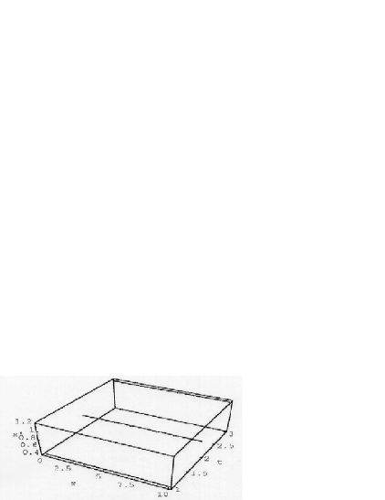
Figure 5.1: $x^{\prime}$-coordinate $(x^{\prime}=\gamma(x-vt))$ of a space-time sector with three values of the Liouville quantized time as seen by a moving observer with velocity $v=2.75\times 10^{8}m/s$, The three space lines are reminiscent of a space having the form of strings. The length of the string is proportional to $x$, the rest frame coordinate of the interacting particle. The width of the string depends on the energy, $\epsilon_{n}$-fluctuations, if any.

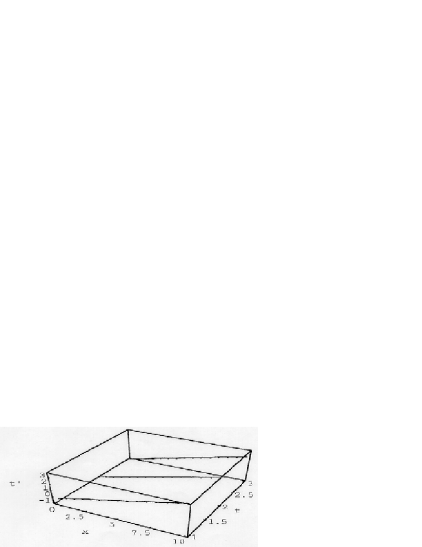
Figure 5.2: The three lines, $t^{\prime}$, $(t^{\prime}=\gamma(t-\beta/c\cdot v))$ give the time for a moving observer in a space-time sector resulting from a Liouville point time-spectrum. The velocity of the observer frame of reference is $v=2.75\times 10^{8}m/s$. The three lines remind us of a space having the form of strings or fibers.

The initial question ’why time changes by steps’ is, thus, answered in the above classical non-relativistic theory of the Liouville equation. The reason for this unexpected fact is that this theory describes observable phenomena only, if two conditions are satisfied:

• The energy distribution function of the particle system is real

• This distribution function is form-invariant with respect to the number of the described particles.

The second condition (5.6) is equivalent to: The action integral of the sum of two particle systems interactiong by means of constant forces is equal to the sum of the action integrals of the separate particle systems, whose particles interact also by means of constant forces.

These two conditions (5.5, 5.6) imposed on the distribution function entail the quantization of the time which then changes by steps. These conclusions, if taken at face value, modify our picture of the time even in a classical theory of atomic systems. They indicate that quantization is a fundamental property of the elements of matter as well as of radiation (Planck black-body radiation).

Figure 5.3: The time spectrum resulting from the additivity and from the reality conditions for the elementary Liouvilian distribution functions. Constant interaction forces and conserved total energy, $E_{N}$, are assumed. If the particle energies, ${\epsilon}_{n}$ fluctuate, then, obviously, the discrete point time-values change to time neighbourhoods of fluctuating measure.

5.3 Determination of Planck’s constant as a verification of chrono-topology

There are several methods for the determination of the value of Planck’s constant. It is natural to expect - as it really is - that this constant which is the ”trade mark” par excellence of quantum physics, should be the result of calculation based typically on some genuine quantum phenomena and on data following from them.

It is just because of this fact that we consider it as extemely surprising that the value of Planck’s constant follows from a classical theory. This theory is Liouville’s equation supplemented with the reality condition and the form invariance requirement of the particle distribution function.

We consider this fact not as an accident and we believe that it entitles us to think about it as an experimental verification of our chrono-topology. We use for the calculation of the $(\lambda=)\hbar$-value expression (5.14)

$$\hbar=\frac{\epsilon_{1}\bar{\tau_{1}}}{2\pi k_{1}}$$ (5.20)

We also consider that the energy $\epsilon_{1}$ is the thermal (translational) energy of the gas molecules

$$\epsilon_{1}=\frac{3}{2}k_{B}T,$$ (5.21)

where $k_{B}=1.38\times 10^{-23}J/K$ is the Boltzmann constant. We take as temperature of the gas $T=300K$. We have still to find $\bar{\tau_{1}}$ and to spcify the quantum number $k_{n}$. We consider first the atomic hydrogen gas, put $k_{n}=1$ and take for the atoms’ average interaction range $R_{\mbox{Atomic}}\approx 1.45\times 10^{-10}m$. The average interaction time, $\bar{\tau_{1}}$, is given by

$$\bar{\tau_{1}}=\frac{2R_{\mbox{Atom.}}}{\sqrt{2}\epsilon_{1}/M_{\mbox{Atom.}}},$$ (5.22)

where the denominator is the average thermal velocity of the atoms with the mass (chemical atomic mass unit $=1.007593$)

$$M_{\mbox{Atom.}} = (1.007593\times 1.65969\times 10^{-27}+9.1083\times 10^{-31})kg$$ (5.23)

$$= 1.6732\times 10^{-27}kg.$$

The above parameters lead for the atomic hydrogen gas to the value

$$\hbar = \frac{\frac{3}{2}k_{B}300\frac{3\times 10^{-10}}{\sqrt{2\frac{3}{2}k_{B}300/(1.6732\times 10^{-27})}}}{2\pi k_{1}}=1.0525\times 10^{-34}Js,$$ (5.24)

$$\hbar = 1.0525\times 10^{-34}Js\mbox{\bf from atomic hydrogen}$$

which is not far from the experimental value.

If we consider molecular hydrogen gas, $M_{\mbox{Molec.}}=2M_{\mbox{Atom.}},R_{\mbox{Molec.}}=2.05\times 10^{-10}m,K_{2}=2,$ then we find

$$\hbar 1.0522\times 10^{-34}Js\mbox{\bf from diatomic hydrogen.}$$ (5.25)

6 Examples of quantum space-time $\bar{M}_{1}^{4}$ -Implications of the chrono-topology

In the preceding section conditions have been given under which time cannot change continuously for a system of particles of given constant total energy interacting via external forces. This formal proof is supporting the experimental evidence that time is a map of changes in observables involved in the fundamental interactions.

6.1 About the time flow in nature

It follows, therefore, that at least under the above restrictive conditions time is quantized. Using the Lorentz transformation it is easy to show that for a moving observer space is also quantized in the form of $\bar{M}_{1}^{4}$.

To see this let us suppose the time is indeed generally quantized and observe the motion of a particle. As long as a time quantum is ’flowing’ we see the particle moving, i.e., changing its position in space. At the end of the time quantum flow, and before the beginning of the next time quantum flow, no position change is observable. Because, if motion were observable, it would be used to define an other time quantum flow which is contrary to the assumption according to which the next time quantum flow has not yet started.

But if a space position change can be observed only during the time quantum flow which can be due only to some fundamental interaction, then, clearly, space is observable as quantized. This can be made clear more formally. We can calculate exactly the structure of a subset of the space, $\bar{M}^{4}_{1}$, provided a set of IPNs is given.

We consider the Lorentz transformation

$$x^{\prime}=\gamma(x-vt)$$ (6.1)

$$t^{\prime}=(t-\beta/cx)$$ (6.2)

in which $(x,t)$ are particle coordinates in the rest frame of reference and $(x^{\prime},t^{\prime})\mathrel{\mathchoice{\raise 0.86108pt\hbox{$\scriptstyle\in$}}{\raise 0.86108pt\hbox{$\scriptstyle\in$}}{\raise 0.86108pt\hbox{$\scriptscriptstyle\in$}}{\raise 0.86108pt\hbox{$\scriptscriptstyle\in$}}}\bar{M}_{1}^{4}$ are the coordinates observed by a moving observer. This transformation is necessary in view of the fact that almost all interacting particles move with respect to the observer.

An example, of how a coordinate $x^{\prime}\mathrel{\mathchoice{\raise 0.86108pt\hbox{$\scriptstyle\in$}}{\raise 0.86108pt\hbox{$\scriptstyle\in$}}{\raise 0.86108pt\hbox{$\scriptscriptstyle\in$}}{\raise 0.86108pt\hbox{$\scriptscriptstyle\in$}}}\bar{M}^{4}_{1}$ appears for fixed $x$ in the rest frame to a moving observer, is given in Fig. 6.1. In this example arbitrary scale factors are used.

It is seen, therefore, that the quantization of the time implies also the quantization of the space by means of the Lorentz transformation. This, however, is not the only consequence for the observer. The discontinuity of the time and the fact that time is embedable in $R^{1}$ produces psychologically for the observer an application of Zermolo’s well-ordering theorem on the generated time quanta, i.e.,

$$\{\tau_{\lambda}\succ\tau_{\lambda+1},\forall\lambda Z^{+}\}$$ (6.3)

This runs as follows: Every new $\tau_{\lambda^{\prime\prime}}\prec\\ tau_{\lambda^{\prime}}$ observed is added (psychologically) to the set $\{\tau_{\lambda},\lambda<\lambda^{\prime}\}$, and this creates the impression of a flow.

Such a flow is not physical, does not exist outside the observer’s mind, and time does not flow in full agreement with Relativity.

6.2 The diameter of the IPNs

In actual experiments we have to put the interaction times whose orders are estimated from experience in Table 6.1 independent of Table 3.1 :

Table 6.1: Orders of magnitude of the in the fundamental interactions according to evidence

Measure of IPN in QED	$10^{-18}s$ to $10^{-14}s$.
Measure of IPN in QCD	$10^{-44}s$ to $10^{-18}s$.

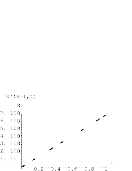
Figure 6.1: The coordinate $x^{\prime}$ according to (6.1a, b) in the space-time topology created by a set of 7 disconnected IPNs $\{\tau_{\lambda}|\lambda=1,2,\ldots 7\}$ due to 7 fundamental interaction events in rest at $x=1$. The $\{\tau_{\lambda}\}$ - and the $x^{\prime}$-neighbourhoods obtainable as orthogonal projections on the corresponding axes are represented in the graph as embedded in the $T$- and in the $\mathchoice{\displaystyle{I\mkern-6.0muR}}{\textstyle{I\mkern-6.0muR}}{\scriptstyle{I\mkern-6.0muR}}{\scriptscriptstyle{I\mkern-6.0muR}}^{1}$-axes for $t$ and $x^{\prime}$ respectively. The measures of and the gaps between the $t$ - and the $x^{\prime}$-neighbourhoods are random. Seen by a moving observer and generated by Lorentz transformation with $v/c=0.916667$. Arbitrary scale factors are used.

6.3 Interactions and observability

Hence, the subset of the Minkowski space ($x=\mbox{const}$) $\bar{M}^{4}_{1}$ for moving observers is quantized with respect to the rest frame of the interacting particles. In view of the above, we prove the following

Proposition 6.1

An non-interacting particle at x=0 in its rest frame of reference is unobservable by all moving observers.

Proof

From (6.1) and from $x=0$, it follows that $x^{\prime}=-\gamma vt$. On the other hand, if $C$ is a constant, the map of the empty set

$$\emptyset\rightarrow C\emptyset=\emptyset,\quad\forall C\mathrel{\mathchoice{\raise 0.86108pt\hbox{$\scriptstyle\in$}}{\raise 0.86108pt\hbox{$\scriptstyle\in$}}{\raise 0.86108pt\hbox{$\scriptscriptstyle\in$}}{\raise 0.86108pt\hbox{$\scriptscriptstyle\in$}}}Rset^{1}$$ (6.4)

is a regular, continuous map of the empty set onto itself. Since $t\mathrel{\mathchoice{\raise 0.86108pt\hbox{$\scriptstyle\in$}}{\raise 0.86108pt\hbox{$\scriptstyle\in$}}{\raise 0.86108pt\hbox{$\scriptscriptstyle\in$}}{\raise 0.86108pt\hbox{$\scriptscriptstyle\in$}}}\tau_{\lambda}=\emptyset$ it follows that $x^{\prime}\mathrel{\mathchoice{\raise 0.86108pt\hbox{$\scriptstyle\in$}}{\raise 0.86108pt\hbox{$\scriptstyle\in$}}{\raise 0.86108pt\hbox{$\scriptscriptstyle\in$}}{\raise 0.86108pt\hbox{$\scriptscriptstyle\in$}}}\emptyset$. The set of the particle coordinates for the moving observer is empty and no particle coordinate is observable. Since the constant $C$ may be any number, we may put $C=\gamma$, and the proof is complete.

Corollary 6.1

No space-time neighbourhood is observable, if there are no interacting particles in it. An application of this corollary is the non-observability of the quarks in the asymptotic freedom state.

6.4 Sheets of space-time

For non-fixed x-coordinates of a particle in a frame of reference, with respect to which the observer moves, a projection of the space $\bar{M}^{4}_{1}$ appears as two distinct sets of world sheets with widths of the orders given in Table 6.1 and random values. The two sets of world sheets lie in two planes forming the angle $\theta=\tan^{-1}(1/\gamma)$.

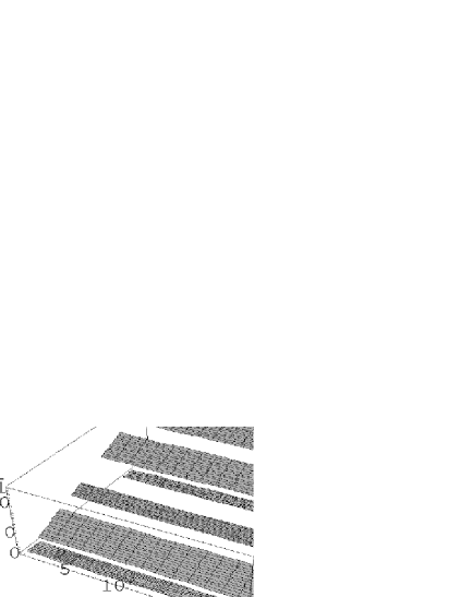
Figure 6.2: World-sheet topology of $\bar{M}^{4}_{1}$ created by four fundamental interaction events in the rest frame of the particle system as observed (after Lorentz transformation) by a moving observer.The widths of the sheets equal to their respective IPNs.The widths of the lower set of sheets equal to the gaps between successive interactions. The IPNs are randomly embedded in the Newtonian $t$-axis and in the Euclidean $x$- and $x^{\prime}$-axes. In this graph the ratio of the velocities is $v/c=0.996667$ and the scale factors are arbitrary.

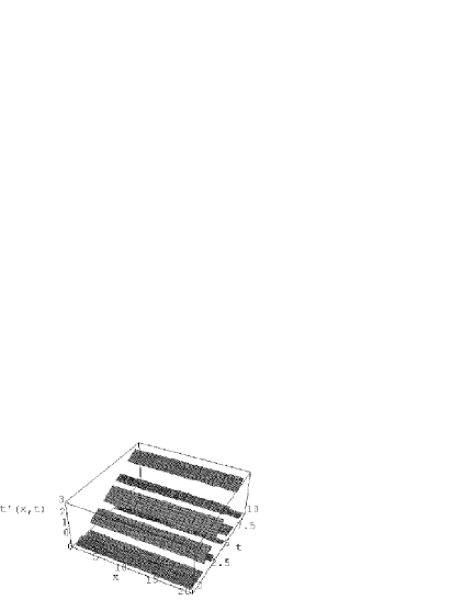
Figure 6.3: $\bar{M}^{4}_{1}$ space-time sheet topology due to five fundamental interaction events in the rest frame generated through Lorentz transformation and seen by a moving observer (Data as in Fig. 6.2). It is evident, how strongly the topology depends on observer’s motion on the number of the interactions taking place in the neighbourhood of the observed system in its rest frame of reference.

Figure 6.4: Three world sheets giving the time for a moving observer with three different velocity ratios, $\beta=v/c$, with respect to the interacting pair of particles due to one single IPN. Arbitrary $x$ and $t$ scale factors. The $t^{\prime}$ scale factor follows from the Lorentz transformation.

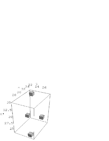
Figure 6.5: Space-time neighbourhoods $\{S_{i}^{\prime}\mathrel{\mathchoice{\raise 0.86108pt\hbox{$\scriptstyle\in$}}{\raise 0.86108pt\hbox{$\scriptstyle\in$}}{\raise 0.86108pt\hbox{$\scriptscriptstyle\in$}}{\raise 0.86108pt\hbox{$\scriptscriptstyle\in$}}}\bar{M}^{4}_{1}|i=1,2,3,4\}$ created by four random IPNs in the rest frame of reference at the fixed point $(y,z)$ and in the time neighbourhoods $\{\tau_{i}|i=1,2,3,4\}$ (arbitrary scale factors).

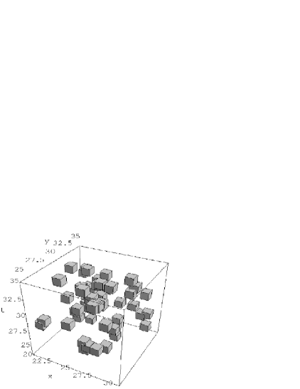
Figure 6.6: Fifty $\bar{M}^{4}_{1}$ space-time neighbourhoods created by an equal number of fundamental interactions in the rest frame of the interacting particles. The continuity is generated through overlapping of adjacent neighbourhoods. For small numbers of partially simultaneous interactions $\bar{M}^{4}_{1}$ is disconnected.

7 Chrono-topology, QFT and irreversibility

Roger Penrose in his celebrated books ”Emperor’s New Mind” and ”Shadows of the Mind” has analyzed virtually all problems of contemporary Physics. A particularly important position takes among them the problem of the reduction of the wave function. He - as now we may see - very clearly states that ”something new must be discovered to solve these problems”. We believe that this is the new time topology, the chrono-topology. Let us start it in a slightly different way: There are two simple, since long puzzling, fundamental facts in physics:

7.1 Boltzmann versus Schroedinger

• The one fact is that Quantum Statistical Mechanics (QSM) is based on essentially, the expression ”$\exp[-E/kT]$ ” or its various formal expressions.

• The second fact is that quantum field theories (QFT) produced hitherto, instead, the factor ”$\exp[-iEt/\hbar]$”.

The deeper reason for the difference of these two kinds of theories resides in the spacetime topology [1]. QFT sits in Minkowski’s topology, $(ict,x,y,z)\mathrel{\mathchoice{\raise 0.86108pt\hbox{$\scriptstyle\in$}}{\raise 0.86108pt\hbox{$\scriptstyle\in$}}{\raise 0.86108pt\hbox{$\scriptscriptstyle\in$}}{\raise 0.86108pt\hbox{$\scriptscriptstyle\in$}}}M^{4}$, QSM is based in the Euclidean topology, $(t,x,y,z)\mathrel{\mathchoice{\raise 0.86108pt\hbox{$\scriptstyle\in$}}{\raise 0.86108pt\hbox{$\scriptstyle\in$}}{\raise 0.86108pt\hbox{$\scriptscriptstyle\in$}}{\raise 0.86108pt\hbox{$\scriptscriptstyle\in$}}}R^{4}$ [53].

Many prominent authors have constructed highly sophisticated theories aiming at paving the way for QSM to move from $R^{4}$ to $M^{4}$. However, a simple problem remains still unsolved: The derivation of the statistical, or the Boltzmann factor, $\exp[-E/kT]$, from QFT in Minkowski’s topology.

1. N. N. Bogolubov introduces in his books [55] the factor in question in a directly ad hoc way.

2. On the other hand, J. Glimm and A. Jaffe [54] obtain the factor $\exp[-E/kT]$ from the Gibbs ensemble, i.e., from an extraneous theory.

3. Similarly, Itzykson and Zuber [53] consider the expression $\exp[-\beta(H-\mu N)]$ in their book on QFT as a priori given, where $\beta=1/kT$ and $\mu$ is the chemical potential.

7.2 Time and temperature - The Wick rotation problem

Other authors apply the Wick rotation, $t\rightarrow t^{\prime}=-it$, on the evolution operator, with a view of coming closer to the desired exponent, $-E/kT$. This means, of course, among other things, that:

• Time becomes complex, i.e., foreign to the physical reality.

• The imaginary part of the universal Newtonian time, is put $Im\{t\}=\beta=1/kT$. It can hardly be physically related with a temperature (which is not as universal as the Newtonian time is) and with the Boltzmann constant of gases ( In fact, the temperature is not related to $(Im\{t\})^{-1}$, but to $\langle\delta(\tau)\rangle^{-1}$, where $\langle\delta(\tau)\rangle$ is the average interaction time in the system of the particles under consideration, [58]). And,

• the Wick rotation, $\{t\rightarrow t^{\prime}=-it|\sqrt{1-(v/c)^{2}}\rightarrow\sqrt{1+(v/c)^{2}}\}$, implies, if $c$ is a reference-frame-independent universal constant, detrimental consequences for special relativity, because it makes $\gamma$ smaller than $1$.

  For general relativity a complex time variable leads to metrics not deriving from gravitational fields [45].

  Despite this fact, Hawking bases his discussion of the black holes on the transformation $t\rightarrow i\tau$ [63]. If the analytic continuation were valid in this particular case from the point of view of physics, then the Minkowski space, and more generally the hyperbolicity would not be necessary for relativity. Relativity, however, cannot be formulated in spaces with posotive definite metrics.

This fact rules out the Wick rotation as a means for deriving the statistical factor $\exp[-E/kT]$ in QFT.

There are also many other, more elaborated approaches [56], to the problem of bringing together QFT and QSM in the same space-time.

In order to give our main application of the chrono-topology we need some definitions. The chrono - topology (helps to eliminate some of the paradoxes and) is based on a very simple and obvious observation that a time not associated with physical changes is neither needed nor definable. It leads to the question: How does change the Hamiltonian for $t\mathrel{\mathchoice{\raise 0.86108pt\hbox{$\scriptstyle\in$}}{\raise 0.86108pt\hbox{$\scriptstyle\in$}}{\raise 0.86108pt\hbox{$\scriptscriptstyle\in$}}{\raise 0.86108pt\hbox{$\scriptscriptstyle\in$}}}\tau$?

7.3 Time and observability

It is interesting to note an unexpected consequence of the chrono-topology: It concerns the variation of the Hamiltonian and the Lagrangian densities for $t\mathrel{\mathchoice{\raise 0.86108pt\hbox{$\scriptstyle\in$}}{\raise 0.86108pt\hbox{$\scriptstyle\in$}}{\raise 0.86108pt\hbox{$\scriptscriptstyle\in$}}{\raise 0.86108pt\hbox{$\scriptscriptstyle\in$}}}\tau$. To clarify the situation we give

Definition 7.1

An IPN, $\tau_{\lambda}$, is an injective map of the $\lambda$-th change, $\Delta O^{j}_{\lambda}$, of the $j$-th observable, $O^{j}$, in $\mathchoice{\displaystyle{I\mkern-6.0muR}}{\textstyle{I\mkern-6.0muR}}{\scriptstyle{I\mkern-6.0muR}}{\scriptscriptstyle{I\mkern-6.0muR}}^{1}$ caused by a fundamental interaction:

$$\Delta O^{j}_{\lambda}\rightarrow f(\Delta O^{j}_{\lambda})=\tau_{\lambda}\mathrel{\mathchoice{\raise 0.86108pt\hbox{$\scriptstyle\in$}}{\raise 0.86108pt\hbox{$\scriptstyle\in$}}{\raise 0.86108pt\hbox{$\scriptscriptstyle\in$}}{\raise 0.86108pt\hbox{$\scriptscriptstyle\in$}}}{\cal T}_{\Lambda}\subset\mathchoice{\displaystyle{I\mkern-6.0muR}}{\textstyle{I\mkern-6.0muR}}{\scriptstyle{I\mkern-6.0muR}}{\scriptscriptstyle{I\mkern-6.0muR}}^{1}.$$ (7.1)

Remark 7.1

The index ”j” in $\Delta O^{j}_{\lambda}$ has been omitted in ${\cal T}_{\Lambda}=\bigcup_{\lambda=1}^{\Lambda}\tau_{\lambda}$, because the knowlegde is not generally desired, from which interaction comes a particular observable change.

However, it is very important to observe that a physical change is not observable inside an IPN, $\tau_{\lambda}$. Because otherwise, a $\tau^{\prime}_{\lambda}\subset\tau_{\lambda}$ would be definable, contrary to the assumption that no $\tau_{\lambda}$ is divisible. This is necessary, since there is no experimental evidence for the possibility to stop a started fundamental interaction.

Consequently, every change, $\Delta O_{\lambda}$, of a physical observable covers the entire IPN, $\tau_{\lambda}$, which is the map of $\Delta O_{\lambda}$ and it can be observed at the end of its creation. This state of affairs gives seemingly rise to a contradiction:

• For $t\mathrel{\mathchoice{\raise 0.86108pt\hbox{$\scriptstyle\in$}}{\raise 0.86108pt\hbox{$\scriptstyle\in$}}{\raise 0.86108pt\hbox{$\scriptscriptstyle\in$}}{\raise 0.86108pt\hbox{$\scriptscriptstyle\in$}}}\tau_{\lambda}H(t),L(t)=\mbox{Constant.}$

• For $t\not\mathrel{\mathchoice{\raise 0.86108pt\hbox{$\scriptstyle\in$}}{\raise 0.86108pt\hbox{$\scriptstyle\in$}}{\raise 0.86108pt\hbox{$\scriptscriptstyle\in$}}{\raise 0.86108pt\hbox{$\scriptscriptstyle\in$}}}\tau_{\lambda}H(t),L(t)=\mbox{Zero.}$

The way out from this dilemma is that $\tau_{\lambda}$ is open and $\bar{\tau_{\lambda}}$ is its closure. Then $H(t)$ and $L(t)$ change for $t\mathrel{\mathchoice{\raise 0.86108pt\hbox{$\scriptstyle\in$}}{\raise 0.86108pt\hbox{$\scriptstyle\in$}}{\raise 0.86108pt\hbox{$\scriptscriptstyle\in$}}{\raise 0.86108pt\hbox{$\scriptscriptstyle\in$}}}\bar{\tau_{\lambda}}\setminus Int\tau_{\lambda}$.

Remark 7.2

$$\mbox{\it Measure of}\quad[\bar{\tau_{\lambda}}\setminus Int\>\tau]=0.$$ (7.2)

This result is of importance to the integration of time-ordered products of non-commuting operators in QFT. Because of (7.1) the operators are time-independent in the interval of integration, [58].

Remark 7.3

Remark 7.1 and Proposition 6.1 offer a possibility to understand, that quarks are not directly observable due to their asymptotic freedom. Particles, in general, are observable only during or after interaction. They are not observable, if they do not interact.

7.4 Randomness in QFT

Definition 7.2

A field ${\cal L}={\cal L}(\phi(x,t),\partial\phi(x,t))\mathrel{\mathchoice{\raise 0.86108pt\hbox{$\scriptstyle\in$}}{\raise 0.86108pt\hbox{$\scriptstyle\in$}}{\raise 0.86108pt\hbox{$\scriptscriptstyle\in$}}{\raise 0.86108pt\hbox{$\scriptscriptstyle\in$}}}\mathchoice{\displaystyle{I\mkern-6.0muR}}{\textstyle{I\mkern-6.0muR}}{\scriptstyle{I\mkern-6.0muR}}{\scriptscriptstyle{I\mkern-6.0muR}}^{1}$ is called a generalized random field, if for ${\cal L}<\xi\mathrel{\mathchoice{\raise 0.86108pt\hbox{$\scriptstyle\in$}}{\raise 0.86108pt\hbox{$\scriptstyle\in$}}{\raise 0.86108pt\hbox{$\scriptscriptstyle\in$}}{\raise 0.86108pt\hbox{$\scriptscriptstyle\in$}}}\mathchoice{\displaystyle{I\mkern-6.0muR}}{\textstyle{I\mkern-6.0muR}}{\scriptstyle{I\mkern-6.0muR}}{\scriptscriptstyle{I\mkern-6.0muR}}^{1}$ a probability $P(\xi)$ is given such that the conditions are fulfilled:

• $P(\xi_{1})=P(\xi_{2})$, if $\xi_{1}=\xi_{2}$,

• $\lim_{\xi\to-\infty}P(\xi)=0$ and $\lim_{\xi\to\infty}P(\xi)=1$,

• $\lim_{\xi\to a-0}P(\xi)=P(a).$

.

Remark 7.4

The limits $(-\infty,\infty)$ in Definition 7.2 above must in our case be replaced by some finite numbers $(a,b)$, because the field, ${\cal L}$, does not become infinite.

Definition 7.3

A generalized random field, $\cal L$, is called infinitely divisible, if for every $\Lambda\mathrel{\mathchoice{\raise 0.86108pt\hbox{$\scriptstyle\in$}}{\raise 0.86108pt\hbox{$\scriptstyle\in$}}{\raise 0.86108pt\hbox{$\scriptscriptstyle\in$}}{\raise 0.86108pt\hbox{$\scriptscriptstyle\in$}}}\mathchoice{{\sevenrm Z}\mkern-9.2mu{\sevenrm Z}}{{\sevenrm Z}\mkern-9.2mu{\sevenrm Z}}{{\sevenrm Z}\mkern-9.2mu{\sevenrm Z}}{{\sevenrm Z}\mkern-9.2mu{\sevenrm Z}}^{+}$the decomposition is possible [57]

$${\cal L}={\cal L}_{1}+{\cal L}_{2}+\ldots+{\cal L}_{\Lambda\kappa},\quad\forall\kappa\mathrel{\mathchoice{\raise 0.86108pt\hbox{$\scriptstyle\in$}}{\raise 0.86108pt\hbox{$\scriptstyle\in$}}{\raise 0.86108pt\hbox{$\scriptscriptstyle\in$}}{\raise 0.86108pt\hbox{$\scriptscriptstyle\in$}}}\mathchoice{{\sevenrm Z}\mkern-9.2mu{\sevenrm Z}}{{\sevenrm Z}\mkern-9.2mu{\sevenrm Z}}{{\sevenrm Z}\mkern-9.2mu{\sevenrm Z}}{{\sevenrm Z}\mkern-9.2mu{\sevenrm Z}}^{+}\mbox{and}x\mathrel{\mathchoice{\raise 0.86108pt\hbox{$\scriptstyle\in$}}{\raise 0.86108pt\hbox{$\scriptstyle\in$}}{\raise 0.86108pt\hbox{$\scriptscriptstyle\in$}}{\raise 0.86108pt\hbox{$\scriptscriptstyle\in$}}}\bar{M}^{4}_{\Lambda_{\kappa}}$$ (7.3)

in which the $\{{\cal L}_{\lambda}(\phi(x,t),\partial\phi(x,t))\}$ are mutually independent, have identical probability distributions, $\{P(\xi_{\lambda})\}$ and are different from zero only in their corresponding IPNs $\tau_{\lambda}\mathrel{\mathchoice{\raise 0.86108pt\hbox{$\scriptstyle\in$}}{\raise 0.86108pt\hbox{$\scriptstyle\in$}}{\raise 0.86108pt\hbox{$\scriptscriptstyle\in$}}{\raise 0.86108pt\hbox{$\scriptscriptstyle\in$}}}{\cal T}_{4}$.

Remark 7.5

According to [58] the decomposition of the field Lagrangian density into an arbitrary number of identical terms with identical probability measures at any point of the space-time is mathematically perfect in the framework of the theory of the generalized and infinitly divisible fields.

However, from the physical point of view such a decomposition would violate all conservation laws in the Minkowski or in the Euclidean space-time. That impossibility disappears in the framework of our many-folded space-time $\bar{M}^{4}_{\kappa}$ for every $\kappa\mathrel{\mathchoice{\raise 0.86108pt\hbox{$\scriptstyle\in$}}{\raise 0.86108pt\hbox{$\scriptstyle\in$}}{\raise 0.86108pt\hbox{$\scriptscriptstyle\in$}}{\raise 0.86108pt\hbox{$\scriptscriptstyle\in$}}}\mathchoice{{\sevenrm Z}\mkern-9.2mu{\sevenrm Z}}{{\sevenrm Z}\mkern-9.2mu{\sevenrm Z}}{{\sevenrm Z}\mkern-9.2mu{\sevenrm Z}}{{\sevenrm Z}\mkern-9.2mu{\sevenrm Z}}^{+}$, since in every IPN the conservation laws hold separately.

$$\mbox{1) }{\cal L}= {\cal L}_{1}+{\cal L}_{2}\quad\quad\quad\quad \mbox{in}\>\bar{M}_{\kappa 2}^{4}$$ (7.4)

$$\mbox{2) }{\cal L}= {\cal L}_{1}+{\cal L}_{2}+{\cal L}_{3}\quad\quad \mbox{in}\>\bar{M}_{\kappa 3}^{4}$$ (7.5)

$$\mbox{3) }{\cal L}= \>\>{\cal L}_{1}+{\cal L}_{2}+\ldots+{\cal L}_{\Lambda_{\kappa}}\> \mbox{in}\>\bar{M}_{\kappa\Lambda_{\kappa}}^{4}.$$

$$\ldots$$

Remark 7.6

The range of $\{{\cal L}_{\lambda}\}$ is determined by the domains both of $x$ and $t$. The domain of $x$ does not depend only on the problem at hand but also on the velocity of the motion of the observer with respect to the rest frame of the interacting particle, since the space topology depends on the topology of the time. The domain of $t$ depends on the nature of the interaction.

Hence, in the defining condition (7.2) above of the generalized random field the limit value $\bar{\xi}$ of $\xi_{\lambda}$, for which the conditions

• $${\cal L}_{\lambda}(\phi(x,t),\partial\phi(x,t)]>\xi_{\lambda}\quad\mbox{for}\quad t\mathrel{\mathchoice{\raise 0.86108pt\hbox{$\scriptstyle\in$}}{\raise 0.86108pt\hbox{$\scriptstyle\in$}}{\raise 0.86108pt\hbox{$\scriptscriptstyle\in$}}{\raise 0.86108pt\hbox{$\scriptscriptstyle\in$}}}\tau_{\lambda}$$ (7.8)

  and

• $$\lim_{\xi\to\bar{\xi}}P(\xi)=1$$

are fulfilled, is not infinite.

The chrono-topology induced by the injective maps in the Definition 3.1 of time consists of IPNs that are structured as follows:

• For systems with few IPNs is time given by the union

  $${\cal T}_{Disconnected}=\bigcup_{\lambda}\tau_{\lambda},\quad\lambda\mathrel{\mathchoice{\raise 0.86108pt\hbox{$\scriptstyle\in$}}{\raise 0.86108pt\hbox{$\scriptstyle\in$}}{\raise 0.86108pt\hbox{$\scriptscriptstyle\in$}}{\raise 0.86108pt\hbox{$\scriptscriptstyle\in$}}}\Lambda.$$ (7.9)

  $\Lambda$ is not very large and are disconnectedly and randomly embedded in the Newtonian time, $\mathchoice{\displaystyle{I\mkern-6.0muR}}{\textstyle{I\mkern-6.0muR}}{\scriptstyle{I\mkern-6.0muR}}{\scriptscriptstyle{I\mkern-6.0muR}}^{1}$. All observers live in $T\subset\mathchoice{\displaystyle{I\mkern-6.0muR}}{\textstyle{I\mkern-6.0muR}}{\scriptstyle{I\mkern-6.0muR}}{\scriptscriptstyle{I\mkern-6.0muR}}^{1}$, but not the atomic, the nuclear and the sub-nuclear particles; they ”live” in ${\cal T}_{Disconnected}$ as defined in their rest frame of reference.

  In order to observe them, a Lorentz transformation is required. The time-space for atomic, nuclear and sub-nuclear particles is the chrono-topological space satisfying the separation axioms of ${\cal T}_{4}$ described in the introduction.

• For systems with $\Lambda$ very large the system-time topology may change radically in the rest frame of reference of the interacting particles.

The union

$${\cal T}_{\Lambda}=\bigcup_{\lambda}\tau_{\lambda},\quad\lambda\mathrel{\mathchoice{\raise 0.86108pt\hbox{$\scriptstyle\in$}}{\raise 0.86108pt\hbox{$\scriptstyle\in$}}{\raise 0.86108pt\hbox{$\scriptscriptstyle\in$}}{\raise 0.86108pt\hbox{$\scriptscriptstyle\in$}}}\Lambda$$ (7.10)

may become equal to the sum of some disconnected spaces ${\cal T}_{Disconnected}$ and of some partitions $\{{\cal P}_{\Lambda_{\kappa}}\mathrel{\mathchoice{\raise 0.86108pt\hbox{$\scriptstyle\in$}}{\raise 0.86108pt\hbox{$\scriptstyle\in$}}{\raise 0.86108pt\hbox{$\scriptscriptstyle\in$}}{\raise 0.86108pt\hbox{$\scriptscriptstyle\in$}}}\mathchoice{\displaystyle{I\mkern-6.0muR}}{\textstyle{I\mkern-6.0muR}}{\scriptstyle{I\mkern-6.0muR}}{\scriptscriptstyle{I\mkern-6.0muR}}^{1}\}$ dense in disconnected subsets, $T$, of $\mathchoice{\displaystyle{I\mkern-6.0muR}}{\textstyle{I\mkern-6.0muR}}{\scriptstyle{I\mkern-6.0muR}}{\scriptscriptstyle{I\mkern-6.0muR}}^{1}$. If the cardinality of $\Lambda$ approaches $\aleph_{0}$, then ${\cal T}_{\Lambda}$ may with high probability, but not certainly, be densely embedded in ${\cal P}_{\Lambda}\mathrel{\mathchoice{\raise 0.86108pt\hbox{$\scriptstyle\in$}}{\raise 0.86108pt\hbox{$\scriptstyle\in$}}{\raise 0.86108pt\hbox{$\scriptscriptstyle\in$}}{\raise 0.86108pt\hbox{$\scriptscriptstyle\in$}}}\mathchoice{\displaystyle{I\mkern-6.0muR}}{\textstyle{I\mkern-6.0muR}}{\scriptstyle{I\mkern-6.0muR}}{\scriptscriptstyle{I\mkern-6.0muR}}^{1}$, and

Cardinality $({\cal T}_{\Lambda})\to{\bf c}$.

7.5 A fundamental quantum proposition

After the above clarifications we shall prove the following Proposition 7.1

• Let ${\cal T}_{\kappa}={\cal T}_{Disconnected}$ be a set of IPNs due to the interaction Hamiltonian density ${\cal H}(\phi(x,t),\partial\phi(x,t))\neq 0$ on the elements of a partition ${\cal P}_{\kappa}\subset{\cal T}_{\kappa}$ of ${\cal T}_{\kappa}$, and

  $${\cal H}(\phi(x,t),\partial\phi(x,t))\equiv 0\quad\mbox{for}\quad t\neq{\cal P}_{\kappa}$$ (7.11)

• Let the Lagrangian have the form

  $${\cal L}(\phi(x,t),\partial\phi(x,t))=\pi(x,t)\partial_{0}\phi(x,t)-{\cal H}(\phi(x,t),\partial\phi(x,t))$$ (7.12)

  for $\tau_{\lambda}\mathrel{\mathchoice{\raise 0.86108pt\hbox{$\scriptstyle\in$}}{\raise 0.86108pt\hbox{$\scriptstyle\in$}}{\raise 0.86108pt\hbox{$\scriptscriptstyle\in$}}{\raise 0.86108pt\hbox{$\scriptscriptstyle\in$}}}{\cal P}_{\kappa}\subset{\cal T}_{\kappa}$ and ${\cal L}(\phi(x,t),\partial\phi(x,t))\equiv 0$ for $t\not\mathrel{\mathchoice{\raise 0.86108pt\hbox{$\scriptstyle\in$}}{\raise 0.86108pt\hbox{$\scriptstyle\in$}}{\raise 0.86108pt\hbox{$\scriptscriptstyle\in$}}{\raise 0.86108pt\hbox{$\scriptscriptstyle\in$}}}{\cal P}_{\kappa}$ with

  $$\pi(x,t)=\frac{\partial}{\partial\partial\phi(x,t)}{\cal L}(\phi(x,t),\partial_{0}(x,t)).$$

• Let $\partial_{0}\phi(x,t)dt=[\phi(x,t+d\tau_{\lambda})-\phi(x,t)]:=d\phi(x,s)$ be the path variation for some $s\mathrel{\mathchoice{\raise 0.86108pt\hbox{$\scriptstyle\in$}}{\raise 0.86108pt\hbox{$\scriptstyle\in$}}{\raise 0.86108pt\hbox{$\scriptscriptstyle\in$}}{\raise 0.86108pt\hbox{$\scriptscriptstyle\in$}}}{\cal P}_{\kappa}$ and every $x\mathrel{\mathchoice{\raise 0.86108pt\hbox{$\scriptstyle\in$}}{\raise 0.86108pt\hbox{$\scriptstyle\in$}}{\raise 0.86108pt\hbox{$\scriptscriptstyle\in$}}{\raise 0.86108pt\hbox{$\scriptscriptstyle\in$}}}\bar{M}_{\kappa}^{4}$.

• Let ${\cal L}(\phi(x,t),\partial\phi(x,t))$ be a generalized, random and infinitely divisible field,

  $${\cal L}={\cal L}_{1}+{\cal L}_{2}+\ldots+{\cal L}_{\kappa}.$$ (7.13)

• Let the field action-integral, $A_{\Lambda}(S_{\kappa})$, be quantized [48] by

  $$A_{\Lambda}(S_{\kappa})=\int_{S_{\kappa}}{\cal L}(\phi(x,t),\partial\phi(x,t))d^{4}x=\pm\hbar\Lambda(j,\sigma),$$ (7.14)

  where

  $$\Lambda(n,\sigma)=\pi\left\{\begin{array}[]{c}n+1/2,\sigma=1\\ n,\sigma=2\end{array}\right\}.$$ (7.15)

  with $n=0,1,2,\ldots$ and $S_{\kappa}\subset\bar{M}_{\kappa}^{4}$.

Then the time evolution operator of the system is

$${\cal U}({\cal T}_{\kappa}) = \exp\langle[(i\hbar)^{-1}\int_{S_{\kappa}}d^{4}x{\cal H}(\phi(x,t),\partial\phi(x,t))\pm i\Lambda(j,\sigma)]$$

$$\quad\times[cos[\Lambda(j,\sigma)]\mp isin[\Lambda(j,\sigma)]]\rangle,$$

and brakes down into two parts:

• non measure preserving (nmp),

  $${\cal U}_{nmp}({\cal T}_{\kappa})=\exp[\frac{(-1)^{n}}{\hbar}\int H(s)ds+\Lambda(n,1)],$$ (7.17)

  or

• unitary (u).

  $${\cal U}_{u}({\cal T}_{\kappa})=\exp[+(i\hbar)^{-1}\int H(s)ds\pm i\Lambda(n,2)],\quad s\mathrel{\mathchoice{\raise 0.86108pt\hbox{$\scriptstyle\in$}}{\raise 0.86108pt\hbox{$\scriptstyle\in$}}{\raise 0.86108pt\hbox{$\scriptscriptstyle\in$}}{\raise 0.86108pt\hbox{$\scriptscriptstyle\in$}}}{\cal P}_{\kappa}$$ (7.18)

Remark 7.7

The proof of the Fundamental Proposition 7.1 will be given on the basis of the solution of the equation governing our time evolution of the state vector $\Psi$ [58] in the time space ${\cal T}_{\kappa}$, a disconnected subset of $\mathchoice{\displaystyle{I\mkern-6.0muR}}{\textstyle{I\mkern-6.0muR}}{\scriptstyle{I\mkern-6.0muR}}{\scriptscriptstyle{I\mkern-6.0muR}}^{1}$.

$$i\hbar\frac{\partial\Psi}{\partial t}=H(t)\Psi(t),\quad t\mathrel{\mathchoice{\raise 0.86108pt\hbox{$\scriptstyle\in$}}{\raise 0.86108pt\hbox{$\scriptstyle\in$}}{\raise 0.86108pt\hbox{$\scriptscriptstyle\in$}}{\raise 0.86108pt\hbox{$\scriptscriptstyle\in$}}}{\cal T}_{\kappa}.$$ (7.19)

The difference between the time evolution equation (7.19) in chrono-topology and in the conventional [53] evolution in time proceeding in the topology of the Newtonian time, $\mathchoice{\displaystyle{I\mkern-6.0muR}}{\textstyle{I\mkern-6.0muR}}{\scriptstyle{I\mkern-6.0muR}}{\scriptscriptstyle{I\mkern-6.0muR}}^{1}$, is that our topology implies (in Penrose’s notation) the process ${\bf U}+{\bf R}$. The Newtonian time topology cannot physically accommodate infinitely divisible fields, because it induces the violation of the conservation laws as a consequence of the infinite divisibility of the Lagrangian and the Hamiltonian densities of the field. Hence, the Newtonian time topology leads only to $\bf U$ evolution according to

$$i\hbar\frac{\partial\Psi}{\partial t}=H(t)\Psi(t),t\mathrel{\mathchoice{\raise 0.86108pt\hbox{$\scriptstyle\in$}}{\raise 0.86108pt\hbox{$\scriptstyle\in$}}{\raise 0.86108pt\hbox{$\scriptscriptstyle\in$}}{\raise 0.86108pt\hbox{$\scriptscriptstyle\in$}}}\mathchoice{\displaystyle{I\mkern-6.0muR}}{\textstyle{I\mkern-6.0muR}}{\scriptstyle{I\mkern-6.0muR}}{\scriptscriptstyle{I\mkern-6.0muR}}^{1}.$$ (7.20)

Proof of the fundamental proposition 7.1

We start the proof by giving the solution of (7.19)

$${\cal U}({\cal T}_{\kappa}) = \{\exp[-i\hbar^{-1}\int{\cal H}(\phi(x^{\prime}),\partial\phi(x^{\prime})){dx^{\prime}}^{4}]\},\quad x^{\prime}\mathrel{\mathchoice{\raise 0.86108pt\hbox{$\scriptstyle\in$}}{\raise 0.86108pt\hbox{$\scriptstyle\in$}}{\raise 0.86108pt\hbox{$\scriptscriptstyle\in$}}{\raise 0.86108pt\hbox{$\scriptscriptstyle\in$}}}{\bar{M}^{4}}_{\kappa}$$ (7.21)

$$= \{\exp[-i\hbar^{-1}\int H(s)ds]\},\quad s\mathrel{\mathchoice{\raise 0.86108pt\hbox{$\scriptstyle\in$}}{\raise 0.86108pt\hbox{$\scriptstyle\in$}}{\raise 0.86108pt\hbox{$\scriptscriptstyle\in$}}{\raise 0.86108pt\hbox{$\scriptscriptstyle\in$}}}{\cal P}_{\kappa}$$ (7.22)

We:

• Combine the above integral with premise 2.

• Write the exponential of the sum of the terms as a product of exponentials of the terms of the sum and

• Develop the factor $\exp[-i\hbar^{-1}\int dx^{4}\partial_{0}\phi(x)\pi(x)]$ in a power series.

$${\cal U}({\cal T}_{\kappa}) = \left\{1+\sum_{\Lambda_{\kappa}=1}^{\infty}\frac{(i\hbar)^{-\Lambda_{\kappa}}}{\Lambda_{\kappa}!}\prod_{\lambda_{\kappa}=1}^{\Lambda}\int_{\bar{M}^{4}_{1}}{\cal L}(\phi(x^{\prime}_{\lambda_{\kappa}}),\partial\phi(x^{\prime}_{\lambda_{\kappa}}))dx^{\prime}_{\lambda_{\kappa}}\right\}$$

$$\times\exp[(-i\hbar)^{-1}\int_{x^{\prime}\mathrel{\mathchoice{\raise 0.60275pt\hbox{$\scriptstyle\in$}}{\raise 0.60275pt\hbox{$\scriptstyle\in$}}{\raise 0.60275pt\hbox{$\scriptscriptstyle\in$}}{\raise 0.60275pt\hbox{$\scriptscriptstyle\in$}}}\bar{M}^{4}_{1}}{\cal L}(\phi(x^{\prime}),\partial\phi(x^{\prime}))d^{4}x^{\prime}]$$

Next, we use premise 3. in the form $\partial_{0}\phi(x^{\prime})d^{4}x^{\prime}=d\phi(q,t^{\prime})d^{3}q$, insert it into (7.5) together with premise 4. and put $\Lambda_{\kappa}=n$ in the $n$-th term of the partition ${\cal P}_{\Lambda_{\kappa}=n}\forall n\mathrel{\mathchoice{\raise 0.86108pt\hbox{$\scriptstyle\in$}}{\raise 0.86108pt\hbox{$\scriptstyle\in$}}{\raise 0.86108pt\hbox{$\scriptscriptstyle\in$}}{\raise 0.86108pt\hbox{$\scriptscriptstyle\in$}}}\mathchoice{{\sevenrm Z}\mkern-9.2mu{\sevenrm Z}}{{\sevenrm Z}\mkern-9.2mu{\sevenrm Z}}{{\sevenrm Z}\mkern-9.2mu{\sevenrm Z}}{{\sevenrm Z}\mkern-9.2mu{\sevenrm Z}}^{+}$.

The $\lambda_{\kappa}$-th integration in (7.5) is carried out on the $\lambda_{\kappa}$-th sector of the $\lambda_{\kappa}$-folded-in-time of the space-time super surface. The result is:

$${\cal U}({\cal T}_{\Lambda_{\kappa}}) = \left\{1+\sum_{\lambda_{\kappa}=1}^{\infty}\frac{(i\hbar)^{-\lambda_{\kappa}}}{\lambda_{\kappa}!}\prod_{\eta=1}^{\kappa}\langle\int_{Q^{3}}d^{3}q^{\prime}\int_{\phi(\underline{q},0)}^{\phi(\overline{q}\delta(\tau_{\eta}))}d\phi(q^{\prime},s^{\prime}_{\eta})\pi(q^{\prime},s^{\prime}_{\eta})\right.$$

$$\left.\times\exp[(-i\hbar)^{-1}\int_{\bar{M}^{4}_{\kappa}}{\cal L}(\phi(x^{\prime}_{\lambda_{\kappa}}),\partial\phi(x^{\prime}_{\lambda_{\kappa}}))d^{4}x^{\prime}_{\lambda_{\kappa}}]\rangle\right\},\quad s^{\prime}_{\eta}\mathrel{\mathchoice{\raise 0.86108pt\hbox{$\scriptstyle\in$}}{\raise 0.86108pt\hbox{$\scriptstyle\in$}}{\raise 0.86108pt\hbox{$\scriptscriptstyle\in$}}{\raise 0.86108pt\hbox{$\scriptscriptstyle\in$}}}\tau_{\eta}.$$

According to the (7.3) of the infinitely divisible fields $\{{\cal L}_{\lambda_{\kappa}}\}$ have all $\lambda_{\kappa}$-independent probability distributions. Using this property and omitting, therefore, the index $\kappa$, in $\lambda_{\kappa}$ under the product sign in (7.5) we can sum-up the series.

Using again the relation

$$\pi(x,t)\partial_{0}\phi(x,t)={\cal L}(\phi(x,t),\partial\phi(x,t))+{\cal H}(\phi(x,t),\partial\phi(x,t))$$ (7.25)

the result after sumation is

$${\cal U}({\cal T}_{\Lambda_{\kappa}}) = \exp[(i\hbar)^{-1}\int_{Q^{3}}d^{3}q^{\prime}d^{3}q\int_{\phi(\underline{q},0)}^{(\overline{q},\delta(\tau))}d\phi(q^{\prime},s^{\prime}_{\eta})\pi(q^{\prime},s^{\prime}_{\eta})]$$ (7.28)

$$\times\exp[(-i\hbar)^{-1}\int_{\bar{M}^{4}_{\kappa}}{\cal L}(\phi(x^{\prime\prime}),\partial\phi(x^{\prime\prime}))d^{4}x^{\prime\prime})]$$

$$= \exp\langle(i\hbar)^{-1}\int_{\bar{M}^{4}_{\kappa}}d^{4}x^{\prime\prime}[{\cal L}(\phi(x,t),\partial\phi(x,t))+{\cal H}(\phi(x,t),\partial\phi(x,t))]$$

$$\times\exp[(-i\hbar)^{-1}\int_{\bar{M}^{4}_{\kappa}}{\cal L}(\phi(x^{\prime}),\partial\phi(x^{\prime}))d^{4}x^{\prime}\rangle$$

$$= \exp\langle(i\hbar)^{-1}\int_{\bar{M}^{4}_{\kappa}}[{\cal L}(\phi(x,t),\partial\phi(x,t))+{\cal H}(\phi(x),\partial\phi(x))d^{4}x]$$

$$\times\{\cos[\hbar^{-1}\int_{\bar{M}^{4}_{\kappa}}{\cal L}(\phi(x^{\prime}),\partial\phi(x^{\prime}))d^{4}x^{\prime}]$$

$$-i\sin[\hbar^{-1}\int_{\bar{M}^{4}_{\kappa}}{\cal L}(\phi(x^{\prime}),\partial\phi(x^{\prime}))d^{4}x^{\prime})]\}\rangle$$

Or, after separation of the real from the imaginary part in the exponent, we get the fundamental formula for the time evolution operator which is a realization of both quantum dynamical processes ${\bf U}$ and ${\bf R}$.

$${\cal U}({\cal T}_{\Lambda_{\kappa})} = \exp\langle\{(i\hbar)^{-1}\int_{\bar{M}^{4}_{\kappa}}d^{4}x[{\cal L}(\phi(x,t),\partial\phi(x,t))+{\cal H}(\phi(x,t),\partial\phi(x,t))]$$ (7.29)

$$\times\cos[\hbar^{-1}\int_{\bar{M}^{4}_{\kappa}}{\cal L}(\phi(x^{\prime}),\partial\phi(x^{\prime}))d^{4}x^{\prime}]$$

$$+ \{(-\hbar)^{-1}\int_{\bar{M}^{4}_{\kappa}}d^{4}x[{\cal L}(\phi(x,t),\partial\phi(x,t))+{\cal H}(\phi(x,t),\partial\phi(x,t))]$$

$$\times\{\mp\sin[\hbar^{-1}\int_{\bar{M}^{4}_{\kappa}}{\cal L}(\phi(x^{\prime}),\partial\phi(x^{\prime}))d^{4}x^{\prime}]\}\}\rangle.$$

7.6 Unitary ${\bf U}$ and Reduction ${\bf R}$ operators

Next, we apply the quantization condition (7.14) on the action integral in the ”cos” and ”sin” expressions of (7.29). The result is

$${\cal U}({\cal T}_{\Lambda_{\kappa}}) = \exp\langle(i\hbar)^{-1}\int_{\bar{M}^{4}_{\kappa}}d^{4}x[{\cal H}(\phi(x,t),\partial\phi(x,t))\pm i\Lambda(j,\sigma)]$$ (7.30)

$$\times\{\cos[\Lambda(j,\sigma)]\mp i\sin[\Lambda(j,\sigma)]\}\rangle.$$

Remembering (7.14) we see that (7.30) can be written as the product of two exponential factors [15], [63]:

• The ${\bf U}$ factor represents the unitary part of the evolution, ${\cal U}_{u}({\cal T}_{{\kappa}})$

• The ${\bf R}$ factor representing the incoherent evolution, ${\cal U}_{nmp}({\cal T}_{{\kappa}})$

This completes the proof of the Fundamental Proposition 7.1.

Remark 7.8

This is the result contemplated by Prigogine and Penrose in their publications. The most interesting feature of (7.30) is that it exhibits simultaneously ${\bf U}+{\bf R}$ properties, just like those postulated by Penrose and required for the implementation of the wave function reduction.

Remark 7.9

A new feature of the evolution operator (7.30) is the spontaneous $\Lambda(n,\sigma)$ renormalization of the action integral in the exponent by means of the term $\Lambda(n,\sigma)$, see also (7.34) and (7.36) below.

7.7 Random fields and functional integral approach

Remark 7.10

Each integral in the series (7.5) is finite, because $\phi$ is a solution of the Euler-Lagrange differential equation satisfying the appropriate boundary conditions. The series converges, because each term is the power of a definite integral. The proof follows by majorization.

Remark 7.11

The continuous parameter $s_{k}^{\prime}$ characterizes the integration path $\mathop{\rm d\vphantom{lg}}\nolimits\phi(q,s)$ in which are the space $[\phi(t),\phi(t+\tau)]$ for the initial and the final values of $\phi(t)$ for $s_{k}^{\prime}=t$, and for $s_{k}^{\prime}=\delta(\tau)$ respectively, while $\phi$ coincides at these values of $s$ with the lower and the upper limits of the $\phi$-path integration.

Corollary 7.1

The contribution ${\cal U}_{\lambda_{\kappa}}({\cal T}_{\kappa})$, to the evolution operator of the path integral in the expansion (7.5) vanishes in the limit $\lambda_{\kappa}\to\infty$.

Proof

The $\lambda_{\kappa}$-th term in equation (7.5) is

$${\cal U}_{{\kappa}}({\cal T}_{\kappa}) = \frac{(i\hbar)^{-\lambda_{\kappa}}}{\lambda_{\kappa}!}\prod_{\eta=1}^{\lambda_{\kappa}}\int_{Q^{3}}d^{3}q\int_{\phi(\underline{q},0)}^{\phi(\overline{q},\delta(\tau_{\eta}))}d\phi(q,s_{\eta})\pi(q,s_{\eta})$$ (7.31)

$$\times \exp[(-i\hbar)^{-1}\int_{\bar{M}^{4}_{\kappa}}{\cal L}(\phi(\phi(x^{\prime}),\partial\phi(x^{\prime}))d^{4}x^{\prime}]$$

The integral over $d\phi$ sums values along all paths and the integral over $dq^{3}$ sums the function $\phi(q,s)$-values along every selected individual paths between the two fixed limit function values $\phi(\underline{q},0)$ and $\phi(\overline{q},\delta(\tau))$ .

The measures in the integrals of the product are well-defined and they exist on the compact supports:

• $\left[\phi(0),\phi(\delta(\tau_{\lambda_{\kappa}}))\right]$, and

• $Q^{3}\subset R^{3}$.

Since the factors $\{f_{\eta}\}$ of the product

$$\prod_{\eta=1}^{\lambda_{\kappa}}\int_{Q^{3}}d^{3}q\int_{\phi(\underline{q},0)}^{\phi(\overline{q},\delta(\tau_{\eta}))}d\phi(q,s_{\eta})\pi(q,s_{\eta})$$

are independent of $\eta$, we have $\prod_{\eta=1}^{\lambda_{\kappa}}f^{\eta}=f^{\lambda_{\kappa}}$, and since the factor $(\lambda_{\kappa}!)^{-1}$ decreases faster than the power, $f^{\lambda_{\kappa}}$, for $\lambda_{\kappa}\to\infty$, there holds true: $\lim_{\lambda_{\kappa}\to\infty}f^{\lambda_{\kappa}}/\lambda_{\kappa}!=0$, and the functional integral does not contribute to the evolution operator. This completes the proof of Corollary 7.1.

Remark 7.12

The ”phase” factor in (7.31) is identical to the one in the Feynman path integral. Differences appear in the functions to be integrated over $d^{3}q$ and over $d\phi(q,s)$. The following correspondances with the Feynman path integral are intringuing:

Remark 7.13

In the limit, $\lim_{\lambda_{\kappa}\to\infty}$, the integrals become functional integrals with the measures

$$Dq \Rightarrow \prod_{\lambda_{\kappa}=1}^{\infty}dq_{\lambda_{\kappa}},\quad q_{\lambda_{\kappa}}\mathrel{\mathchoice{\raise 0.86108pt\hbox{$\scriptstyle\in$}}{\raise 0.86108pt\hbox{$\scriptstyle\in$}}{\raise 0.86108pt\hbox{$\scriptscriptstyle\in$}}{\raise 0.86108pt\hbox{$\scriptscriptstyle\in$}}}Q^{3}\subset R^{3}$$ (7.32)

and

$$Dp \Rightarrow \prod_{\eta}^{\infty}\pi(\phi(q,s_{\eta}),\partial\phi(q_{\eta},s))d\phi(q,s_{\eta})$$ (7.33)

for $\phi(q,s_{\eta}),\pi(\phi(q,s),s_{\eta}),\partial\phi(q,s_{\eta})\mathrel{\mathchoice{\raise 0.86108pt\hbox{$\scriptstyle\in$}}{\raise 0.86108pt\hbox{$\scriptstyle\in$}}{\raise 0.86108pt\hbox{$\scriptscriptstyle\in$}}{\raise 0.86108pt\hbox{$\scriptscriptstyle\in$}}}L^{2}$.

7.8 Functional approach and uncertainty principle

In any way the contributions of these integrals, similar to the Feynman path integrals, are zero because of the normalization factor, $\lambda_{\kappa}!$ in the limit $\lambda_{\kappa}\to\infty$ (Corollary 7.1).

The functional integral features in (7.5) appear similar or in a slightly more general form, and the theory yields in case $\lambda_{\kappa}=n,\forall n\mathrel{\mathchoice{\raise 0.86108pt\hbox{$\scriptstyle\in$}}{\raise 0.86108pt\hbox{$\scriptstyle\in$}}{\raise 0.86108pt\hbox{$\scriptscriptstyle\in$}}{\raise 0.86108pt\hbox{$\scriptscriptstyle\in$}}}\mathchoice{{\sevenrm Z}\mkern-9.2mu{\sevenrm Z}}{{\sevenrm Z}\mkern-9.2mu{\sevenrm Z}}{{\sevenrm Z}\mkern-9.2mu{\sevenrm Z}}{{\sevenrm Z}\mkern-9.2mu{\sevenrm Z}}^{+}$ the exponential form of the Hamiltonian well-known from QFT. The similarities and the differences between the present theory and the Feynman path integral are shown in 7.1.

Table 7.1: Comparison of the Feynman path integral properties with those of the present theory and some statistical and quantum properties.

	Feynman		Present work
Spatial measure:	$Dq=\prod_{k=1}^{\infty}dq_{k}$	$\Leftrightarrow$	$\prod_{k=1}^{\infty}d^{3}q_{k}$
Functional measure:	$Dp=\prod_{k=1}^{\infty}dp_{k}$	$\Leftrightarrow$	$\prod_{k=1}^{\infty}\pi(\phi(q_{k},s),\partial\phi(q_{k},s))d\phi(q_{k},s)$
Normalization:	?	$\Leftrightarrow$	$1/k!$
Uncertainty Principle:	no		yes
Gibbs ensemble:	no		yes

In the case $j=(2n+1)/2$ in (7.30) the exponential becomes real and has a form reducible to the form known from QSM.

We, thus, have two evolution operators: One preserving the norm and one changing it.

The canonical momentum, $\pi(q,s)$, enters as a weight factor - not as differential under integration. This makes the integration measures compatible with Heisenberg’s Uncertainty Principle in case of quantization of the field action.

7.9 Statistical ensembles and temperature in QFT

The measure preserving evolution is implemented through

$${\cal U}_{u}(\delta(\tau),0)=\exp[(i\hbar)^{-1}\int_{\bar{M}^{4}_{\kappa}}d^{4}x{\cal H}(\phi(x),\partial\phi(x))\mp i\pi n],n=0,1,2,\ldots.$$ (7.34)

If the evolution does not preserve the norm of the state vector, then it is given by

$${\cal U}_{nmp}(\delta(\tau),0) = \exp[\langle\frac{(-1)^{n}}{\hbar}\int_{S_{\lambda}}{\cal H}(\phi(x),\partial\phi(x))\mp\pi(n+1/2)\rangle],$$ (7.36)

$$n=0,1,2,3,\ldots.$$

If the state vector, $\Psi$, is expanded in a series of eigenstates of the Hamiltonian, and ${\cal U}_{u}(\delta(\tau),0)$ or ${\cal U}_{nmp}(\delta(\tau),0)$ acts on $\Psi$, then (7.34) and (7.36) become respectively:

$$\exp[-i\sum_{\lambda=1}^{\Lambda}E_{\lambda}\cdot\delta(\tau_{\lambda})/\hbar\mp i\pi n],$$ (7.37)

and

$$\exp[(-1)^{n}\sum_{\lambda=1}^{\Lambda}E_{\lambda}\cdot\delta(\tau_{\lambda})/\hbar\mp\pi(n+1/2)].$$ (7.38)

Corollary 7.2

The temperature of a system of particles interacting via a fundamental interaction is inversely proportional to the average diameter of the interaction proper-time neighbourhoods $\langle\delta(\tau)\rangle_{\kappa}$ defined by

$$\langle\delta(\tau)\rangle_{\kappa}=\Lambda^{-1}_{\kappa}\sum_{\lambda=1}^{\Lambda}\delta(\tau_{\lambda_{\kappa}})$$ (7.39)

Proof

We divide and multiply the sum in the exponent of

$$\exp[(-1)^{n}\sum_{\lambda_{\kappa}=1}^{\Lambda_{\kappa}}E_{\lambda}\cdot\delta(\tau_{\lambda_{\kappa}})/\hbar+\pi(n+1/2)]$$

by $\sum_{\lambda_{\kappa}=1}^{\Lambda_{\kappa}}\delta(\tau_{\lambda_{\kappa}})$ and we write for the time averaged energy per particle the expression

$$\langle\delta(\tau_{\lambda_{\kappa}})\rangle_{\kappa}\cdot\langle E\rangle_{\kappa}\cdot\Lambda_{\kappa}=\left(\frac{\sum_{\lambda_{\kappa}=1}^{\Lambda_{\kappa}}E_{\lambda_{\kappa}}\cdot\delta(\tau_{\lambda_{\kappa}})}{\sum_{\lambda_{\kappa}=1}^{\Lambda_{\kappa}}\delta(\tau_{\lambda_{\kappa}})/\Lambda_{\kappa}}\right)\cdot\sum_{\lambda_{\kappa}=1}^{\Lambda_{\kappa}}\delta(\tau_{\lambda_{\kappa}})/\Lambda_{\kappa}.$$

The factors (7.37, 7.38) entering the state vector after the action of ${\cal U}_{nmp}(\delta(\tau),0)$ are essentially the Boltzmann statistical factors [48], if the system temperature is defined by

$$T_{\kappa}=\frac{\hbar}{\langle\delta(\tau)\rangle_{\kappa}k_{B}},$$

where $k_{B}$ is the Boltzmann constant.

The average frequency of the collisions, $f_{coll}$, is given by

$$f_{coll}=\langle\delta(\tau)\rangle_{\kappa}^{-1}$$

and it allows to give a definition of the temperature in the framework of quantum field theory.

This completes the proof of Corollary 7.2.

Remark 7.13

The main features of the present temperature definition are:

• Relativity is respected by avoiding the Wick rotation.

• The canonical ensemble follows from the QFT.

• The temperature is related to the collision frequency [58] in the framework of QFT.

Remark 7.14

It is remarkable that the averaging of the energy is by the structure of the theory over the time these energies are possessed by the particles, but not over the number of the particles. This is quite natural, because, if an energy value is possessed during zero time by a particle, it contributes zero to the average energy of the system.

7.10 Einstein – Bohr. Both were right

Some authors believe that Bohr was right and Einstein wrong or vice versa ( e.g. [11], [63] ) in their disput about the statistical character of quantum mechanics.

It has been proved in the framework of chrono-topology, that both were right. The reason for this fact was, that Einstein’s statement, according to which God does not play dice, regarded the quantum equations of motion (Schroedinger, Dirac, etc.) per se , i.e., inside a single IPN, and in this case God does not play dice inside $\tau$. Indeed, the quantum equations are per construction not statistical. However, the description of the quantum phenomena cannot be done fot $t\mathrel{\mathchoice{\raise 0.86108pt\hbox{$\scriptstyle\in$}}{\raise 0.86108pt\hbox{$\scriptstyle\in$}}{\raise 0.86108pt\hbox{$\scriptscriptstyle\in$}}{\raise 0.86108pt\hbox{$\scriptscriptstyle\in$}}}\tau$. The ewason is that observation is conventionally done in ${\cal T}_{\kappa}$. But for $t\mathrel{\mathchoice{\raise 0.86108pt\hbox{$\scriptstyle\in$}}{\raise 0.86108pt\hbox{$\scriptstyle\in$}}{\raise 0.86108pt\hbox{$\scriptscriptstyle\in$}}{\raise 0.86108pt\hbox{$\scriptscriptstyle\in$}}}{\cal T}_{\kappa}$ the interpretation of the solutions of the quantum equations becomes necessarily statistical [48].

Bohr’s statement, on the other hand, regarded quantum physics results as a whole, because quantum physic’s arena is not $\tau$ itself. The physical ”playground” is rather ${\cal T}_{\kappa}=\bigcup\tau_{\lambda}$, and the space-time, $\bar{M}^{4}_{\kappa\lambda_{k}appa}$, resulting from it according to Einstein’s relativity.

Moreover since $\{\delta(\tau_{\lambda})\}$ are within limits random numbers, an averaging process takes place to give any measured value. This is the way in which the statistical character of quantum mechanics emerges. So much, as far as time is concerned. Regarding the space coordinates, a similar explanation is true: Since in every interaction the impact parameter is a random length, a random component is introduced in each space coordinate. This, again, makes necessary an averaging process on the deterministic solution of the wave equation.

It becomes, thus, clear [48] that both Bohr and Einstein were right in their respective statements. Their difference was in their premises, which can be discerned only in the framework of chrono-topology.

8 Solving the measument problem - The reduction of the state vector

In what consists the reduction of the wave function? According to Einstein ’Gott wuerfelt nicht’. We, of course, are allowed to ’wuerfeln’ and we shall do it for a while.

However, before doing that we shall pay tribute of due honor to all great scientists, who came infinitesimally close, in their publications, to our solution of the problem of the present section. They made observations and remarks extremely approximating the solution we provide in this work and they showed to us the way for obtaining the solutions of several puzzles in quantum theory. Of all those scientists we shall make particular reference to two whose contributions seems of the greatest importance from our point of view:

The great forerunners of this work are Ilya Prigogine and Roger Penrose.

8.1 The irreversibility question

Prigogine made the following remarkably lucid statements in his by now famous book “From being to becoming” [10] : ’It is difficult to believe that the observed irreversible processes such as viscosity, decay of unstable particles and so forth, are simply illusions caused by lack of knowledge or by incomplete observation … . Therefore, irreversibility must have some basic connection with the dynamical nature of the system’.

Sofar we fully agree with Prigogine’s philosophy. The continuation of his syllogism goes as follows: ’… because for simple types of dynamical systems the predictions of classical and quantum mechanics have been remarkably well verified’.

Despite the remarkable verification of quantum mechanics our remarks are two:

• The time structure is ill understood in general dynamics.The reason is that always the interaction time, $\tau_{\lambda}$, has been identified in quantum dynamics with the Newtonian time having the topology of $\mathchoice{\displaystyle{I\mkern-6.0muR}}{\textstyle{I\mkern-6.0muR}}{\scriptstyle{I\mkern-6.0muR}}{\scriptscriptstyle{I\mkern-6.0muR}}^{1}$ . We abandon the topology of $\mathchoice{\displaystyle{I\mkern-6.0muR}}{\textstyle{I\mkern-6.0muR}}{\scriptstyle{I\mkern-6.0muR}}{\scriptscriptstyle{I\mkern-6.0muR}}^{1}$ and introduce instead the notion of chrono-topology consisting of unions of IPNs.

• The predictions are in fact remarkably well verified, except for the description of the measurement process and the irreversibility.

Continuing, Prigogine concludes-and this was of great help to us: ’ The problems of unity of science and of time are so intimately connected that we cannot treat the one without the other’.

8.2 The reduction question

Let us now see Penrose’s most clear guidance in the matter of our problem [15]: ’The quantum measurement problem is to understand, how the procedure ${\bf R}$ can arise-or effectively arise - as a property of a large-scale behavior in ${\bf U}$-evolving quantum systems. The problem is not solved merely by indicating a possible way in which an ${\bf R}$-like behavior might conceivably be accommodated. One must have a theory providing some understanding of the circumstances under which (the illusion ?) ${\bf R}$ comes about’.

This is exactely the way we followed in constructing our theory which simultaneously describes the ${\bf U}$-and the ${\bf R}$-processes in quantum field theory with exactly the same accuracy. Here is, however, an additional aspect: In our approach ${\bf R}$ comes about not only for large-scale systems, but also for single quantum particles, thus enabling us to solve the Schroedinger cat’s puzzle too.

The first and basic idea came to us from [1] and a first derivation has been given in [48, 58]. In Sec. 7 of the present paper the full derivation is given. Penrose continues: ’It appears that people often think of the precision of quantum theory as lying in its dynamical equations, namely ${\bf U}$. But ${\bf R}$ itself is also very precise in its prediction of probabilities, and unless it can be understood, how it comes about, one does not have a satisfactory theory’.

In the second statement by Penrose it seems to us that the freedom is contained that ${\bf R}$ be or not be a consequence of the same dynamics. We show that our theory gives both ${\bf U}$ and ${\bf R}$ with exactly the same precision and we demonstrate that ${\bf U}$ and ${\bf R}$ come about by means of quantizing the field action-integral.

8.3 Experience and expectation

After the above due clarifications we are ready to ’play dice’ and answer the questions entailed by the problem posed at the beginning of this section: In studying the game, we may do a small calculation and figure out what we have to expect after throwing a dice.

The probability is $1/6$ for getting any number from $1$ to $6$:

Calculated final state of the dice $=$

$$F=1/6\times(\mbox{get 1})+1/6\times(\mbox{get 2})+\cdots+1/6\times(\mbox{get 6}).$$ (8.1)

This is, of course, the result of a calculation of what is foreseen. There is no relationship whatsoever - causal or acausal - with the future decision for doing or not doing the experiment. It is an empirical statistical fact independent of whether we play or not play dice in future. The result of the calculation (8.1) will not change after throwing the dice. The equation remains unaffected, if the dice shows, e.g., $5$ or anything else. After having played dice we know the fact, e.g., and we may represent it by,

$$\mbox{Exp(erimental)Res(ults)}=F_{\mbox{exp.}}=1\times\>\mbox{(got 5)},\>\mbox{and}\>0\times\>\mbox{(got all others)},$$ (8.2)

but our equation (8.1) remains, of course, unaltered. ’Calculation’ and ’fact’ are related only in our brains. $F$ in (8.1 is a theory-devised construct for predictions based on empirical data, representing the possibilities for many different (in this case $6$) outcomes of dicing. Equation (8.2) is of a different character. It is constructed to represent a posteriori one single fact: The outcome of one single experiment and there can be no question about any reduction.

Next, we may make more perfect our theory of playing dice and we construct an operator, ${\cal D}$, describing our dice playing. We want it to describe the dice-throwing. This will be done by appllying ${\cal D}$ on $F$. The result of this application will, if our theory is a good one, be equal to $F_{exp}$ . It will induce the reduction on the paper, not in Nature.

If $F$ and ${\cal D}$ represent exactly the system and our action on it respectively, then

$${\cal D}F=1\times\mbox{(got 5)},\quad\mbox{and}\quad 0\times\mbox{( got all others)}\>=F_{exp},$$ (8.3)

${\cal D}$ describes exactly our way of taking and throwing (the dynamics) the dice in the particular experiment above. It has nothing to do with a statistical theory (Einstein).

Let us see a little more precisely what this means in the particular experiment: It means:

• A definite motion of the hand of the particular experimentalist, implemented through a definite preparation and function of his hand-muscle system.

• A definite motion of his arm, implemented through a definite preparation and function of the arm-muscle system.

• A definite electrical conductance or polarization and function of the neural synapses system etc. leading from the brain to the fingers of his hand.

• A certain preparation and function of his brain, conscious to a certain degree of the programme to be carried out. This degree of consciousness may differ from one experimentalist to an other, and to an experimentalist in different experiments.

• A certain interaction between his ’will’ and his brain in order that the latter prepares itself and acts.

These five steps of preparation are subject to large uncertainties, both macroscopic and quantum mechanical.The magnitudes of the uncertainties increase with increasing index in the above enumeration scheme from i) to v).

Moreover, what is virtually fully undefined is the description in physical terms of the interaction between the ’will’ and the brain. Hence, the construction of the operator ${\cal D}$ for experiments of the above type is not an easy task for today’s Science and Technology. The difficulty is localized in the lack of knowledge in the quantum description of the individual human functions. However, in most physics experiments participation of human body s functions at the realization of experiment’s crucial parts is to a well-defined degree excluded. Also, the human brain is involved only in the preparation of the experiment, in the analysis and in the interpretation of the ExpRes. Hence, the construction of the operator ${\cal D}$ in quantum mechanical experiments is in general easier and feasible.

Similar is the situation in quantum theory. Long experience and deep insight by Euler and Lagrange and by many others have shown two series of facts:

• If we construct a certain function, $\cal L$, appropriate to the problem at hand and we apply a variational principle, we derive an equation (Schroedinger) containing some operators $\{{\cal D}\}$ which corresponds to our problem.

• The actions of $\{{\cal D}\}$ on a certain function $F=f(\Psi)$ ($\Psi$ is a wave function) describe satisfactorily the ExpRes, and the construction of our function, $\cal L$, is correct.

Hence, if our theory is correct, then we must have:

$${\cal D}f(\Psi)=ExpRes.$$

Some authors believe that the construction of $\cal D$ is impossible in the framework of the theory of Schroedinger’s equation in such a way that the above equation is not true in the sense of (8.3) and R must come from extraneous agents. We shall try to examine the actual situation in the framework of our present chrono-topology. We shall try first to clarify the situation through the following definitions.

8.4 Nature is not divisible in classical and quantal

Definition 8.1

Every experiment in systems ranging from atomic to sub-nuclear is divided into two parts:

• The experiment proper which involves one fundamental physical interaction, relies on the laws of quantum physics and characterizes ${\cal D}$ (${\cal D}$-process).

• The process of making a quantum interaction visible may rely either on quantum laws or on laws of classical physics or on both and is not characteristic of $\cal D$ (non-$\cal D$-process).

• There are many ways, $X\mathrel{\mathchoice{\raise 0.86108pt\hbox{$\scriptstyle\in$}}{\raise 0.86108pt\hbox{$\scriptstyle\in$}}{\raise 0.86108pt\hbox{$\scriptscriptstyle\in$}}{\raise 0.86108pt\hbox{$\scriptscriptstyle\in$}}}\{W_{i},P_{i}\mid i=1,2,\ldots\}$, for implementing an ExpRes appropriate either to wave properties, $W_{i}$, or to particle properties, $P_{i}$. but not simultaneously to both .

• Part ii) can be implemented in any one of the possible ways, $X\mathrel{\mathchoice{\raise 0.86108pt\hbox{$\scriptstyle\in$}}{\raise 0.86108pt\hbox{$\scriptstyle\in$}}{\raise 0.86108pt\hbox{$\scriptscriptstyle\in$}}{\raise 0.86108pt\hbox{$\scriptscriptstyle\in$}}}\{W_{i},P_{i}\mid i=1,2,\ldots\}$, and, hence, $X$ is not an uniquely chacteristic part of the experiment proper.

• The elements of the set $\{ExpRes(X)\},\forall X\mathrel{\mathchoice{\raise 0.86108pt\hbox{$\scriptstyle\in$}}{\raise 0.86108pt\hbox{$\scriptstyle\in$}}{\raise 0.86108pt\hbox{$\scriptscriptstyle\in$}}{\raise 0.86108pt\hbox{$\scriptscriptstyle\in$}}}\{W_{i},P_{i}\mid i=1,2,\ldots\}$, are equivalent:

  $$ExpRes(X)\Leftrightarrow ExpRes(Y),\forall(X,Y)\mathrel{\mathchoice{\raise 0.86108pt\hbox{$\scriptstyle\in$}}{\raise 0.86108pt\hbox{$\scriptstyle\in$}}{\raise 0.86108pt\hbox{$\scriptscriptstyle\in$}}{\raise 0.86108pt\hbox{$\scriptscriptstyle\in$}}}\{W_{i},P_{i}\mid i=1,2,\ldots\}.$$ (8.4)

Remark 8.1

According to Definition 8.1 an experiment in quantum physics consists of a fundamental interaction between two given quantum entities, on the one hand a structured or an elementary particle, and on the other hand, a measuring apparatus, whose specifically active part may be another structured, elementary particle or field.

Remark 8.2

The process of making the ExpRes macroscopically visible is a separate step, exterior to the quantum measurement.

Remark 8.3

The view that in every quantum physics experiment we have the interaction of a quantum system with a classical apparatus (black box approach) does not correspond to the facts according to the present work. Because the method used for the indication of the result of a fundamental interaction is not essential to the interaction itself. As a rule, the ExpRes is obtained by means of: photomultipliers, scintillators, Wilson chambers, Geiger-Mueller detectors, recoil detectors, spark detectors and other well-known elementary particle detectors.

The way to magnify a quantum interaction does not play an essential part in the interpretation per se and to the construction of the operator $\cal D$, as (8.4) makes clear.

Having the above clarifications in mind we can see that in constructing our operator, $\cal D$, implementing the measuring process in a quantum experiment, we do not need any input extraneous to the interacting quantum system. One thing, which, however, is not extraneous to the quantum interacting system, is the preparation of the experiment. We must, further, specify, what we understand under ’preparation of the experiment’.

Definition 8.2

The preparation of a quantum experiment consists of two processes:

• The preparation of the states of the elementary or structured particle systems determined to interact with one another and subsequently to interact with the active part of the measuring apparatus.

• Preparation of the active part of the measuring apparatus and of its state to measure either a particle property, $P_{i}$ ,or a wave property, $W_{i}$.

Definition 8.3

• A quantum measurement is the experimental determination of one or more quantum transitions in the prepared system. The transition may consist in the change(s) of some observable(s)during a fundamental interaction in the prepared quantum system and the active part proper of the measuring apparatus.

• The preparation of an experiment influences the system to be measured in such away that it increases the probabilities for one or a few of the possible outcomes, constituting the ExpRes to be determined relative to all other possible outcomes.

Remark 8.4

Accordingly, we understand that the critical part of a quantum experiment is an interaction between two particles, or between a particle and a field, or between two fields causing the evolution of the system whose an observable is to be determined within its corresponding IPN either in the interacting system rest frame of reference or in observer’s system of reference .

8.5 Schroedinger’s equation produces ${\bf R}$

Proposition 8.1

The reduction of the state vector describing a quantum measurement is effected by the evolution operator ${\cal D}(\tau)$ with the interaction Hamiltonian, $H(t)$, appropriate to the preparation of the experiment for $t\mathrel{\mathchoice{\raise 0.86108pt\hbox{$\scriptstyle\in$}}{\raise 0.86108pt\hbox{$\scriptstyle\in$}}{\raise 0.86108pt\hbox{$\scriptscriptstyle\in$}}{\raise 0.86108pt\hbox{$\scriptscriptstyle\in$}}}\tau$. ${\cal D}(\delta(\tau))$ reduces the probability amplitudes $\{C_{n}(0)\}$ of all components of the initial state vector

$$\Psi(x)=\sum_{n}C_{n}(0)u_{n}(x)$$

representing the system under measurement, except the ones $\{C_{\alpha}(0)\mid\alpha=1,2,\ldots,K<\infty\}$ corresponding to the observables $\{O_{\alpha}\mid\alpha=1,2,\ldots,K<\infty\}$ to be obtained in the ExpRes.

Proof

The operator ${\cal D}(\delta(\tau))$ can be taken equal either to evolution operator ${\cal U}_{nmp}(\delta(\tau))$ or to ${\cal U}_{u}(\delta(\tau))$ depending on the case. In the present case we identify ${\cal D}(\delta(\tau))={\cal U}_{nmp}(\delta(\tau))$.

$${\cal U}_{nmp}(\delta(\tau)) = \exp\langle(i\hbar)^{-1}\int_{M_{\kappa}^{4}}d^{4}x{\cal H}(\varphi(x,t),\partial\varphi(x,t)\pm i\Lambda(j,\sigma))$$ (8.5)

$$\times(\cos(\Lambda(j,\sigma))\pm i\sin(\Lambda(j,\sigma)))\rangle)$$

before quantization.

The expression for the preparation of the experiment preparation comes about through the selection of the appropriate quantum numbers in $\Lambda(j(n),\sigma)$ following the quantization of the field action-integral (8.5). The kind of quantization to be applied becomes clear from the expectation to have a non-measure-preserving evolution or a unitary evolution, i.e., we expect to measure substantial changes in the relative probability measures of the components characterizing the system before and after the measurement with respect to the remaining components.

Carrying out the multiplication of the quantities in the brakets of the exponent in (8.5) we see that the above requirement is fulfilled according to (7.14), if one puts

$$\Lambda(n,\sigma)=\pi(n+1/2),\sigma=1.$$ (8.6)

From (8.6) it follows after application of (8.5) on the state vector that

$${\cal U}_{nmp}(\delta(\tau))\Psi(x)$$

$$= \exp\langle\left[\frac{(-1)^{n}}{\hbar}\int_{M_{\lambda}^{4}}d^{4}x{\cal H}(\varphi(x,t),\partial\varphi(x,t)\mp\Lambda(j(n),\sigma))\right]\rangle\Psi(x)$$

$$= \sum_{n=1}^{\infty}\exp\langle\left[\frac{(-1)^{n}}{\hbar}\int_{M_{\lambda}^{4}}d^{4}x{\cal H}(\varphi(x,t),\partial\varphi(x,t))\mp\Lambda(j(n),\sigma)\right]\rangle C_{n}(0)u_{n}(x)$$

$$= \sum_{n=1}^{m}\exp\langle\left[(-\hbar)^{-1}\int_{M_{\lambda}^{4}}d^{4}x{\cal H}(\varphi(x,t),\partial\varphi(x,t))-(j(n)+1/2)\right]\rangle C_{n}(0)u_{n}(x)$$

$$+ \sum_{\alpha=1+m}^{m+K}\exp\langle\left[(+\hbar)^{-1}\int_{M_{\lambda}^{4}}d^{4}x{\cal H}(\varphi(x,t),\partial\varphi(x,t))+(\alpha(n)+1/2)\right]\rangle C_{\alpha}(0)u_{\alpha}(x)$$

$$+ \sum_{n=1+m+K}^{\infty}\exp\langle\left[(-\hbar)^{-1}\int_{M_{\lambda}^{4}}d^{4}x{\cal H}(\varphi(x,t),\partial\varphi(x,t))-(j(n)+1/2)\right]\rangle C_{n}(0)u_{n}(x).$$

By appropriately choosing the respective action-integral values, i.e., $\{j(n)\}$ in each class of states in the sum, we obtain that only the intermediate sum survives. The corresponding exponents are the sums of two positive numbers. The first and the third sums above become as small as we please by taking the differnces in the respective exponents sufficiently small in comparison with the smallest term in the sum, as implies the preparation of the experiment $\alpha\mathrel{\mathchoice{\raise 0.86108pt\hbox{$\scriptstyle\in$}}{\raise 0.86108pt\hbox{$\scriptstyle\in$}}{\raise 0.86108pt\hbox{$\scriptscriptstyle\in$}}{\raise 0.86108pt\hbox{$\scriptscriptstyle\in$}}}[1+m,n+K]$.

$${\cal U}_{nmp}(\delta(\tau))\Psi(x) \approx \sum_{\alpha=1+m}^{K}exp\left[(+\hbar)^{-1}\int_{M_{\lambda}^{4}}d^{4}x{\cal H}(\varphi(x,t),\partial\varphi(x,t)+(\alpha(n)+1/2))\right]$$ (8.7)

$$\quad\times C_{\alpha}(0)u_{\alpha}(x)$$

If the set of the orthonormal functions $\{u_{n}(x)\}$ are eigefunctions of the energy operator, then (8.7) can be simplified in the form

$${\cal U}_{nmp}(\delta(\tau))\Psi(x) = \sum_{\alpha=1+m}^{K}\exp\left(\hbar^{-1}E_{\alpha}\delta(\tau)+(\alpha(n)+1/2))\right)C_{\alpha}(0)u_{\alpha}(x)$$

$$= \sum_{\alpha=1+m}^{K}C_{\alpha}(\delta(\tau))u_{\alpha}(x),$$

where

$$C_{\alpha}(\delta(\tau))=\exp\left(\hbar^{-1}E_{\alpha}\delta(\tau)+(\alpha(n)+1/2))\right)C_{\alpha}(0).$$

Obviously, the probability coefficients for the surviving states are much larger than the rest of them

$$\mid C_{\alpha}(\delta(\tau))\mid^{2}\gg\mid C_{n}(\delta(\tau))\mid^{2}\forall\alpha\mathrel{\mathchoice{\raise 0.86108pt\hbox{$\scriptstyle\in$}}{\raise 0.86108pt\hbox{$\scriptstyle\in$}}{\raise 0.86108pt\hbox{$\scriptscriptstyle\in$}}{\raise 0.86108pt\hbox{$\scriptscriptstyle\in$}}}[1,K],\forall n\mathrel{\mathchoice{\raise 0.86108pt\hbox{$\scriptstyle\in$}}{\raise 0.86108pt\hbox{$\scriptstyle\in$}}{\raise 0.86108pt\hbox{$\scriptscriptstyle\in$}}{\raise 0.86108pt\hbox{$\scriptscriptstyle\in$}}}\mathchoice{{\sevenrm Z}\mkern-9.2mu{\sevenrm Z}}{{\sevenrm Z}\mkern-9.2mu{\sevenrm Z}}{{\sevenrm Z}\mkern-9.2mu{\sevenrm Z}}{{\sevenrm Z}\mkern-9.2mu{\sevenrm Z}}^{+}\setminus[1,K].$$ (8.8)

and the proof Proposition 8.1 is complete.

Remark 8.5

This is the expected result corresponding to the preparation of the experiment and implying the reduction, ${\bf R}$, of the wave function after the experiment. It is seen that ${\bf R}$ is an integral part of quantum dynamics and it does not need the presence of any extraneous agents. The numbers $\alpha(n),j(n)$ and $K$ depend on the preparation and the kind of interaction in the experiment. $\{\alpha(n)$ may be large, $\{j(n)\}$ are correspondingly of the orders of $\{E_{n}\}$. $K$ is in most experiments equal to $1$.

Remark 8.6

The novum in the above proof is:

• It is seen that ${\bf R}$ does not imply necessarily reduction to one single sate, but to any finite number, $K$, of final states.

• The reduced states are not fully extinguished! They simply become of very small relative probability.

• The result ii) stresses the statistical appearence of quantum theory which is traced back to the chrono-topology.

9 Schroedinger’s cat is only alive before he dies and only dead after he lived

9.1 Cats in physics

There is a considerable literature about cats in physics. To us are known at least two famous cats: The first was Lewis Carroll’s cat in the Wonderland of Alice’s Adventures. The other one, equally important for quantum theory, is Schroedinger’s cat.

Are they really so important for physics? We do not know for sure. In any way, they have been both important for some people for some time.

The importance of Alice’s cat consisted in that he was able to leave his charmed smile in the air as his signature - alike the quarks in the QCD of the jets.

Schroedinger’s cat did not smile. Some important people wanted him for some decades dead and alive at the same time. We will examine here, if his sentence was just, and, if not, we shall try to revise it.

Let us see what this means for quantum theory and let us briefly recall the story: There is a hermitically closed room and a glass bottle of an extremely strong poison in it. A hammer hangs above the bottle and can be activated for its purpose by means of the decay of one nucleus from a quantity of a radioactive isotope put in the mechanism [50].

The life of the cat has exactly the same chances with the life of the (first) nucleus to decay, and the state vector of the nucleus consists of two components. The one component stands for an unstable nucleus (before decay) and corresponds to alive cat.

The other component of the state vector represents a stable nucleus (after decay) and is a proof for the dead cat.

The linear superposition of the components is meant to represent a natural state of affairs as far as the nucleus is concerned. But it is considered as a paradoxical business in cat’s case.

Nevertheless, it is considered as thoroughly plausible that, in principle, the same state vector represents both the state of the nucleus and cat’s state. It is thereby clear that the nucleus may consist of a few (for the Tritium 4) particles, whilest the cat is made of some $10^{25}$ particles.

Besides, it has not been possible to demonstrate until today, that the state vector of about $10^{25}$ particles does not acquire additional (collective) unknown properties beyond those of the state vector of the Tritium. These properties might profoudly change the character of the wave function by shifting the values of its importance parameters.

9.2 The action quantization saves the cat

Questions like the above will be left aside and we shall apply the theory developed in the previous sections to demostrate that the cat can be only alive before he dies, because of the poison in the bottle and he can be only dead after he definitely has finished his life for any reason whatsoever.

We do that by means a two-component state vector. The component number $n=1$ represents the unstable nucleus before radioactive decay. The component number $n=2$ represents the nucleus after the emission of a quantum.

Further assumptions, e.g., about the wave function of the cat will not be done. Also no assumptions are necessary about the wave functions of the hammer, of the bottle, of the poison and the mechanical parts of a device interacting with our quantum system, because they are not a part of the quantum system whose solution is sought.

The quantum mechanically crucial phase of the experiment beyond the radioactive decay of one of the unstable nuclei is not the engineering mechanism, but rather the interaction of the radiation quantum with one or more nuclei of the detector which will produce the electric pulse, required for the macroscopic activation of the mechanism.

We trust that, if one nucleus decays, the hammer will move, and the rest will be in accordance with the engineering design. Our decision about the ”sentence” of the cat will result from the proof of the following

Proposition 9.1

Let

$$\Psi(x,0)=\sum_{n=1}^{2}C_{n}(0)u_{n}(x,0)$$ (9.1)

be the two-state vector at time $t=0$ of a nucleus with two possible bound states of its Hamiltonian, $H(t)$, with binding energies $E_{1},E_{2}<0$ :

• State $n=1$ represents the initial unstable nucleus before the radioactive decay ($t=0$) and is associated with a very large probability with respect to the state $n=2$.

• State $n=2$ represents the stable nucleus after the radioactive decay ($t=\delta(\tau)$) and is associated with a very large probability with respect to the state $n=1$.

$$\left|C_{1}(t=0)\right|>>\left|C_{2}(t=0)\right|.$$ (9.2)

Then, the transition from state $n=1$ to state $n=2$ is effected by means of the non-measure preserving time evolution operator with ” $\pm$” in the front of the integral in the exponent:

$${\cal U}_{nmp}(\delta(\tau))=\exp\langle[\pm\hbar^{-1}\int_{\bar{M}^{4}_{\lambda}}d^{4}x{\cal H}(\phi(x,t),\partial\phi(x,t))+\Lambda(j,\sigma)]\rangle,\quad\sigma=1$$ (9.3)

with the interaction Hamiltonian

$$H=\int_{\bar{M}^{4}_{\lambda}}d^{4}x{\cal H}(\phi(x,t),\partial\phi(x,t))$$ (9.4)

within the IPN, $\tau_{\lambda}$. The probability for the state $n=1$ at $t=\delta(\tau)$, i.e., at the end of the nuclear emission process is very small, while that for the state $n=2$ is very large after the transition:

$$\left|C_{2}(t=\delta(\tau))\right|>>\left|C_{1}(t=\delta(\tau))\right|.$$ (9.5)

Remark 9.1

Relations (9.2) express the fact that the cat is alive with very high, virtually $1$, probability and dead with very small, virtually zero, probability. Relations (9.5) express the converse case, namely that the cat is dead with very high, virtually $1$, probability and alive with very small, virtually zero, probability. The seeming small uncertainty about ”alive” and about ”dead” does not need to confuse us, because this is the natural state of affaires in quantum mechanics.

For example, according to statistical mechanics, and, also, to the Poincare recurrence theorem, there exists a vanishingly small probability that the set of atoms, of which consisted Einstein short before his death, recombine to give the living Einstein. This probability is virtually zero.

Proof

The interaction (9.4) (fixed by its structure) inducing the transition of the unstable nucleus from the state characterized by (9.2) to the state characterized by (9.5) constitutes the ”preparation” of the experiment according to Definitions 8.1 and 8.3 and gives the appropriate value to the field action integral, $+\Lambda(j,1)$. The sign ”$+$” with large $\Lambda(j,1)$ corresponds to the ”present” state of the system, because it gives to the action integral the maximum value and maximum probability to the state. The sign ”$-$” determines the state which is the ”absent” state, because its action, $-\Lambda(j,1)$, gives a very small, virtually zero, probability.

If we act with the operator 9.3 on the state vector 9.1 we get

$$\sum_{n=1}^{2} \exp\langle[\frac{(-1)^{n}}{\hbar}\int_{\bar{M}^{4}_{\lambda}}d^{4}x{\cal H}(\phi(x,t),\partial\phi(x,t))\mp\Lambda(j(n),\sigma)]\rangle C_{n}(0)u_{n}(x,0)$$

$$= \exp\langle\frac{(-1)^{n}}{\hbar}\int_{\bar{M}^{4}_{\lambda}}{\cal H}(\phi(x,t),\partial\phi(x,t))-\Lambda(j(1),\sigma)]\rangle C_{1}(0)u_{1}(x,0)$$ (9.6)

$$\quad+\exp\langle+\hbar^{-1}\int_{\bar{M}^{4}_{\lambda}}{\cal H}(\phi(x,t),\partial\phi(x,t))+\Lambda(j(2),\sigma)]\rangle C_{2}(0)u_{2}(x,0)$$

$$= \exp\rangle[-\hbar^{-1}|E_{1}|\delta(\tau)-\Lambda(j(1),\sigma)]\rangle C_{1}(0)u_{1}(x,\delta(\tau))\quad\quad\quad$$ (a)

$$\quad+\exp\rangle[+\hbar^{-1}|E_{2}|\delta(\tau)+\Lambda(j(2),\sigma)]\rangle C_{2}(0)u_{2}(x,\delta(\tau))\quad\quad\quad$$ (b)

$$= C_{1}\delta(\tau)u_{1}(x,\delta(\tau))+C_{2}\delta(\tau)u_{2}(x,\delta(\tau))\;\quad\quad\quad\quad\quad$$ (c)

$$\approx C_{2}\delta(\tau)u_{2}(x,\delta(\tau))\;\quad\quad\quad\quad\quad$$ (d) (9.7)

From 9.7 we conclude by taking appropriate values for $j(1)$ and $j(2)$ that

$$|C_{2}\delta(\tau)u_{2}(x,\delta(\tau))|^{2} = |C_{2}(0)u_{2}(x,0))|^{2}\exp[+2/\hbar|E_{2}|\delta(\tau)+2j(2)+1]$$ (9.8)

$$\gg |C_{1}(0)u_{1}(x,0))|^{2}\exp[-2/\hbar|E_{1}|\delta(\tau)-2j(1)+1]$$

From 9.8 it follows that

$$|C_{2}(\delta(\tau))u_{2}(x,\delta(\tau))|^{2}>>|C_{1}(\delta(\tau))u_{1}(x,\delta(\tau))|^{2}$$ (9.9)

and this completes the proof of Proposition 9.1.

Remark 9.2

The values of $\pm\Lambda(j(n))$ which determine the probabilities of the corresponding components of the state vector are determined by the interaction 9.4 effecting the transition of the nucleus. In case it is very large, it describes a ”clear cut” state of the system.

Remark 9.3

Equations 9.7 prove that that the state vector does not evolve any more after the transition, because $\delta(\tau),E_{1},E_{2}$ are constants.

Remark 9.4

If the probability, $p_{2l}$, of the state for the living Schroedinger cat after the decay of the unstable nucleus is vanishingly small in comparison with the probability, $p_{2d}\gg p_{2l}$, for the dead cat, it is experimentally impossible to observe the alive cat after he died with very high probability.

Hence, there is no Schroedinger’s cat paradox in the framework of the theory of the Schroedinger equation.

Remark 9.5

The solution given in the present section opens new aspects for all problems concerning quantum systems with two or few levels possible. This is a novel aspect of R and it is in full agreement with the statistical nature of the wave function.

10 The non-decay of the wave packet

Our basic principle in chrono-topology is that interactions are the causes of all changes in the universe. No change whatsoever is possible without an interaction. Accordingly, fluctuations also should be due to some sort of interaction. The fluctuations in the density of a gas are due to particular ’constellations’ of a number of interacting pairs of atoms with particular values of the scattering angles. We propose to consider the wave packet decay from this point of view.

10.1 Attempts at avoiding decay

There exist rather ambitious mathematical theories making various attempts to reconcile the non-decay of the particle with the decay of the wave packet representing it. The problem consists in that the wave packet does decay in the absence of interactions in the Newtonian time topology, while the particle does not decay.

One of the theories endeavoring to eliminate the decay of the wave packet in the Newtonian time topology proposes some gravitational agents [59]. These agents result to the restauration of the decaying wave packet implied by quantum theory. However, there is no indication about a relation of the agents with any physical action directing them exclusively towards decaying wave packets and preventing them of acting on non-decaying waves too. Another theory postulates for the same purpose the spontaneous multiplication of the wave packet (function) by a strongly picked Gaussian function in definite time intervals to cancel the calculated decay of the wave packet [60].

These theories refrain from giving in any way neither the locations of the large number of the required computers to implement the multiplication of all travelling wave packets in the universe, corresponding to the particles of the cosmic radiation and to the beam particles in the accelarator laboratories or in the nuclear reactors. Also they give no indication, if, for example, instead of a mathematical multiplication of the wave packet, there occurs a physical amplification, e.g., like the amplification of an electrical pulse in an electronic device. These are questions which in our view should also be answered, if these theories claim the qualification of completeness.

It is, finally, interesting to note that E. P. Wigner proceeded to accepting the existence of an influence on the unconscious matter by any living matter in such a way as to change the U action of the time evolution operator to an R action [61].

All three explanations of the factual non-decay of the particle corresponding to a decaying wave packet, make appeal to effects which physically are difficult to explain in the framework of the valid laws. This entitles us to look for other, simpler explanations.

10.2 The flowing Newtonian time at the root of the confusion

The solution of the above problem in the framework of our chrono-topology appears in comparison with the above mentioned very sophisticated theories as a rather trivial excercise. In this context it would appear surprising, if the wave packet did really decay in the absence of any interactions.

As in the problem of the measurement in quantum mechanics, it will be, here too, assumed that the decay of the wave packet, whenever it occurs, is described exclusively by the evolution operator. To see this we consider an orthonormal and complete set of eigenfunctions $\{u_{n}\left|n=1,2,\ldots\right.\}$ of the Hamiltonian $H(t)$ and we write for the state vector the expression for $t=0$

$$\Psi(x,0)=\sum_{n=1}^{\infty}C_{n}u_{n}(x),$$ (10.1)

where $x\mathrel{\mathchoice{\raise 0.86108pt\hbox{$\scriptstyle\in$}}{\raise 0.86108pt\hbox{$\scriptstyle\in$}}{\raise 0.86108pt\hbox{$\scriptscriptstyle\in$}}{\raise 0.86108pt\hbox{$\scriptscriptstyle\in$}}}\bar{M}^{4}_{1}$ is the particle coordinate in its rest frame of reference, $S$.

10.3 Let us see, what happens

The details of the wave packet construction are described in books on quantum mechanics and they are not repeated here. We shall, instead, prove only the following

Proposition 10.1

• Let $\Psi(x,0)$ be the wave packet representing a particle in the point $x$ at the time $t=0$ in its rest-frame of reference.

• Let $\{u_{n}(x),E_{n},\left|n=1,2,\ldots\right.\}$ represent an orthonormal, complete system of eigenfunctions of the Hamiltonian ${\cal H}(\phi(x),\partial\phi(x))$ and the corresponding energy eigenvalues.

• Let ${\cal U}_{u}({\cal T}_{\Lambda})$ be the unitary time evolution operator implementing the changes on $\Psi(x,0)$ implied by ${\cal H}(\phi(x),\partial\phi(x))$.

• The rest-frame of reference of the particle is a macroscopic material body with which a moving observer’s detector may interact via any quanta exchange and in this way determine the position of the particle without in any way disturbing it or its wave packet.

Then,

• The wave packet remains unchanged in its rest-frame of reference without interactions.

• The wave packet does not decay for an observer moving with respect to the rest-frame of reference of the particle without interactions.

• The wave packet changes form under an U and - a fortiori - under an ${\bf R}$ interaction.

Proof

• We act on $\Psi(x,0)$ with our unitary time evolution operator, ${\cal U}_{u}({\cal T}_{\Lambda})$:

  $${\cal U}_{u}({\cal T}_{\Lambda})\Psi(x,0)$$

  $$= \sum_{n=1}^{\infty}\exp\langle[(i\hbar)^{-1}\int_{\bar{M}^{4}_{\lambda}}d^{4}x{\cal H}(\phi(x,t),\partial\phi(x,t))\pm\Lambda(n,\sigma)]\rangle C_{n}u_{n}(x)$$

  $$= \sum_{n=1}^{\infty}\exp\langle[(i\hbar)^{-1}E_{n}\delta(\tau)\pm i\Lambda(n,\sigma)]\rangle C_{n}u_{n}(x)$$

  where the time integration is taken inside a single IPN, $t\mathrel{\mathchoice{\raise 0.86108pt\hbox{$\scriptstyle\in$}}{\raise 0.86108pt\hbox{$\scriptstyle\in$}}{\raise 0.86108pt\hbox{$\scriptscriptstyle\in$}}{\raise 0.86108pt\hbox{$\scriptscriptstyle\in$}}}\tau$. We take for convenience the unitary time evolution operator, because of the periodic bounrary conditions imposed on the orthonormal set $\{u_{n}\left|n\mathrel{\mathchoice{\raise 0.86108pt\hbox{$\scriptstyle\in$}}{\raise 0.86108pt\hbox{$\scriptstyle\in$}}{\raise 0.86108pt\hbox{$\scriptscriptstyle\in$}}{\raise 0.86108pt\hbox{$\scriptscriptstyle\in$}}}\mathchoice{{\sevenrm Z}\mkern-9.2mu{\sevenrm Z}}{{\sevenrm Z}\mkern-9.2mu{\sevenrm Z}}{{\sevenrm Z}\mkern-9.2mu{\sevenrm Z}}{{\sevenrm Z}\mkern-9.2mu{\sevenrm Z}}^{+}\right.\}$ used in (a)).

  Considering $\{u_{n}\left|n\mathrel{\mathchoice{\raise 0.86108pt\hbox{$\scriptstyle\in$}}{\raise 0.86108pt\hbox{$\scriptstyle\in$}}{\raise 0.86108pt\hbox{$\scriptscriptstyle\in$}}{\raise 0.86108pt\hbox{$\scriptscriptstyle\in$}}}\mathchoice{{\sevenrm Z}\mkern-9.2mu{\sevenrm Z}}{{\sevenrm Z}\mkern-9.2mu{\sevenrm Z}}{{\sevenrm Z}\mkern-9.2mu{\sevenrm Z}}{{\sevenrm Z}\mkern-9.2mu{\sevenrm Z}}^{+}\right.\}$ and replacing the sum $\sum_{n}$ by the integral $\int dn$ we find, for

  $$\Lambda(n,\sigma),\sigma=2,$$

  and

  $$E_{n}=\frac{\hbar^{2}n^{2}}{2m},n\mathrel{\mathchoice{\raise 0.86108pt\hbox{$\scriptstyle\in$}}{\raise 0.86108pt\hbox{$\scriptstyle\in$}}{\raise 0.86108pt\hbox{$\scriptscriptstyle\in$}}{\raise 0.86108pt\hbox{$\scriptscriptstyle\in$}}}\mathchoice{{\sevenrm Z}\mkern-9.2mu{\sevenrm Z}}{{\sevenrm Z}\mkern-9.2mu{\sevenrm Z}}{{\sevenrm Z}\mkern-9.2mu{\sevenrm Z}}{{\sevenrm Z}\mkern-9.2mu{\sevenrm Z}}^{+},$$

  by the usual procedure [62] the wave packet form

  $$\Psi_{\pm}(x,\delta(\tau))=(2\pi)_{x}^{-1}(\Delta x+\frac{i\hbar\delta(\tau)}{2m\Delta x})^{-1/2}\exp[-\frac{(x\pm 1)^{2}}{(\Delta x)^{2}+2i\hbar\delta(\tau)/m}].$$ (10.3)

  Expression (10.3) proves that the wave packet cannot decay in time in its rest frame of reference, since, according to Axiom III the IPN, $\tau$, without interaction represents simply the epmpty set, and $\delta(\tau)=0$.

  This proves assertion a).

  

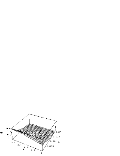
  Figure 10.1: A minimal wave packet decaying in Minkowski’s $S$ space-time (lines in the plane t,wp). In chrono-topology there is no time-flow in absence of interactions, and, consequently, the wave packet conserves its initial form (any constant curve in the plane x,wp). Arbitrary scale factors.

• We consider the Lorentz transformation with the velocity, $v$, of the observer along the positive $x$-direction. Then, we have the expressions:

  $$x = \gamma(x^{\prime}-vt),t=\gamma(t^{\prime}-(\beta/c)x^{\prime}),\mbox{(a)}$$

  $$x^{\prime} = \gamma(x+vt),t^{\prime}=\gamma(t+(\beta/c)x),\mbox{(b)}$$ (10.4)

  and we get the transformed wave packet

  $$\Psi_{\pm}(x,\delta(\tau)) \rightarrow \Psi^{\prime}_{\pm}(x^{\prime},\delta(\tau^{\prime}))$$ (10.5)

  $$= (2\pi)_{x}^{-1/2}(\Delta x+\frac{i\hbar\gamma(t^{\prime}+(\beta/c)x^{\prime})}{2m\Delta x})^{-1/2}$$

  $$\quad\times\exp[-\frac{\gamma(x^{\prime}+vt^{\prime})\pm 1)^{2}}{(\Delta x)^{2}+2i\hbar\gamma(t^{\prime}+(\beta/c)x^{\prime})/m}].$$

  Let us now see what are the domains of variation of $x^{\prime}$ and $t^{\prime}$: In absence of an interaction in S the particle conserves: $x=\rho=$ Constant, and $t=0$. For an observer in $S^{\prime}$ there follows from (b)):

  $$x^{\prime}=\gamma\rho=\mbox{ {\it Constant}, and}\quad t^{\prime}=\beta\cdot\rho\;c=\mbox{ {\it Constant}.}$$

  Hence, the wave packet appears to the moving observer as having a different form, but it does not change, it does not decay, if not subject to an interaction.

  This proves b).

• Let $\rho$ be the constant position of the particle in $S$. Since the particle is subject to an interaction its proper time $t$ takes values in $\tau,t\mathrel{\mathchoice{\raise 0.86108pt\hbox{$\scriptstyle\in$}}{\raise 0.86108pt\hbox{$\scriptstyle\in$}}{\raise 0.86108pt\hbox{$\scriptscriptstyle\in$}}{\raise 0.86108pt\hbox{$\scriptscriptstyle\in$}}}\tau$.

We know, in addition, that the diameter of the IPN, $\tau$, is finite, $\delta(\tau)=\delta<\infty$.

From (b)) we find

$$x=\rho,\mbox{and}\;\tau\equiv(0,\delta).$$

Consequently, for constant $B_{i},i=1,2,3,4$

$$-\infty<B_{1}=\gamma\rho\leq x^{\prime}\leq\gamma(\rho+(\beta/c)\delta)=B_{2}<+\infty\;\quad\mbox{(a)}$$ (10.6)

and

$$-\infty<B_{3}=\gamma\rho\leq t^{\prime}\leq\gamma(\delta+(\beta/c)\rho)=B_{4}<+\infty\;\quad\mbox{(b)}$$

Since the independent variables $x^{\prime}$ and $t^{\prime}$ in (10.5) change by finite amounts, the wave packet changes by a finite amount its form, but it does not decay any more in $S^{\prime}$, given that its interaction is of finite duration.

This proves assertion c) , and the proof of Proposition 10.1 is complete.

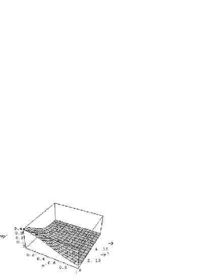
Figure 10.2: The minimal wave packet of Figure 10.1 seen from a moving frame of reference $S^{\prime}$ in Minkowki’s space-time. If an interaction is present with, say $\delta(\tau)=10^{-15}$ seconds, one can see the wave packet deformation in a plane ( $t^{\prime},wp^{\prime}$). To appreciate the amount of the wave packet change in two parallel planes ($x^{\prime},wp^{\prime}$) compare $\delta(\tau)$ with the length, $6\cdot 10^{-9}$ seconds, of the $t^{\prime}$- axis segment.

Remark 10.1

The double sign in (10.3) represents a degree of freedom and it stems from the double sign in the quantization of the action integral, $\pm\Lambda$. The shift of the wave packet center comes from the non-vanishing action-integral.

Remark 10.2

Since the proof does not depend on the form of the wave packet (10.1), it follows that all wave packets do not decay, if not subject to an interaction. This is the situation in the case of soliton waves.

Remark 10.3

If the interaction Hamiltonian is of such a structure, that it changes the nature of the particle described by the wave packet under discussion, this will follow from (a)) under the action of non-measure preserving evolution operator , ${\cal U}_{nmp}({\cal T}_{\lambda})$. In this case also we shall have one or more wave packets behaving according to Proposition 10.1.

11 Conclusions and discussion

There have been numerous investigations into the nature and the structure of time in the history of physics and philosophy. Already in ancient times, Plato, Aristotle, St. Augustine have written essays trying to understand, what is that, we call the time.

The references given are only a tiny sample of the world literature on time. There have been reported very important and less important ideas on the time issue, to all of whom we cannot do due justice with an appropriate reference.

Until recent times of our ending millenium, however, the discussion about the nature of time was mainly of a philosophical character and, hence, it could not have any important repercussions on the advances and on the results of physics and technology.

With the advent of relativity as well as of quantum theory a vast literature on the time has been, and is still today being, produced in the framework of theoretical and of mathematical physics.

In the cases, of these two disciplines of physics, however, the ideas about the time are not so harmless as they were in the case of philosophy: As a consequence, a considerable number of paradoxes and awkward situations arised due, on the one hand, to the fundamental character of these important disciplines, and, on the other hand, due to the assumed structure of time - as we now believe to be able to see. To be specific, some of the most impressive paradoxes in physics are:

• The measurement problem in quantum physics.

• The long-standing impasse ’Time reversal invariance of QFT-Irreversibility in macroscopic Nature’.

• The decay of the wave packet in absence of interactions.

• The catastrophies in QFT.

• The Schroedinger cat.

• The twin paradox in relativity.

• The time machines, etc.

After an examination of the fundamental concepts of physics, we believe that all these and many other paradoxes are due to the character and the topological structure of the time assumed in physics. The topological properties of the time, tacitly introduced both in relativity and in quantum theory, are those of the Newtonian universal time. One should remember here the requirement of relativity according to which every space point has its own time. Also, Dirac’s proposal that each particle should have its own time variable has not helped to abondon the natural topology of the line as the topology of the time in atomic and sub-atomic physics.

The trouble is not limited on the topology of time. Beyond that, the human physiology and in particular the neural structure of the human body and of the brain contributed considerably to the confusion of the time mystery.It lead to the assignment to the time of a phantastic property: The flowing.

Let us be a little more precise and explain, how the feeling of the time flowing comes about in the framework of our chrono-topology: According to our theory of the time structure (Sec. 3) is directly related to the changes occuring in nature and recorded in any way by the nervous system of the observer. Every elementary change generates a time neighbourhood $\tau_{\lambda}$. The next interaction proper-time neighbourhood, $\tau_{\lambda+1}$, necessarily starts before or after the ending of the preceding one and ends later, if it is to be distinguished from the first. The successively observed non-overlapping changes create the sense of ordering. Zermelo’s well-ordering theorem finds here a practical application in the production of the feeling of the flowing time.

The excitations by the successive changes of, both the external and the internal world, act in succession on the neural system of the observer, and give to him the impression of something running, the apparent time property of flowing.

On the other hand, the feeling of the time continuity is created by the finite ability of the observer to discriminate closely adjacent $\{\tau_{\lambda}\mid\forall\lambda\mathrel{\mathchoice{\raise 0.86108pt\hbox{$\scriptstyle\in$}}{\raise 0.86108pt\hbox{$\scriptstyle\in$}}{\raise 0.86108pt\hbox{$\scriptscriptstyle\in$}}{\raise 0.86108pt\hbox{$\scriptscriptstyle\in$}}}I\subset\mathchoice{{\sevenrm Z}\mkern-9.2mu{\sevenrm Z}}{{\sevenrm Z}\mkern-9.2mu{\sevenrm Z}}{{\sevenrm Z}\mkern-9.2mu{\sevenrm Z}}{{\sevenrm Z}\mkern-9.2mu{\sevenrm Z}}^{+}\}$ of a large number (some Avogadro-number-interaction-proper-time) of successive neighbourhoods, created in observer’s brain by his observable environment (external and internal), when the gaps between $\tau_{\lambda}$ and $\tau_{\lambda+1}$ forall $\lambda\mathrel{\mathchoice{\raise 0.86108pt\hbox{$\scriptstyle\in$}}{\raise 0.86108pt\hbox{$\scriptstyle\in$}}{\raise 0.86108pt\hbox{$\scriptscriptstyle\in$}}{\raise 0.86108pt\hbox{$\scriptscriptstyle\in$}}}\mathchoice{{\sevenrm Z}\mkern-9.2mu{\sevenrm Z}}{{\sevenrm Z}\mkern-9.2mu{\sevenrm Z}}{{\sevenrm Z}\mkern-9.2mu{\sevenrm Z}}{{\sevenrm Z}\mkern-9.2mu{\sevenrm Z}}^{+}$ are large enough.

Since time, alike the space, does not flow, the view that a wave-packet should decay in absence of interactions, appears in our chrono-topology as a paradox, seen that time changes only as long as the interaction is going on.

As far as phenomena are concerned, whose durations are larger than the interaction proper time neighbourhood diameter of the intervening fundamental interaction, the physical results are perfectly described in physics, and experiment and theory are in very good agreement.

However, as soon as the distances between successive single elementary phenomena approach the limit of the IPNs perception proper-time, then troubles set in.

Many, extremely subtle affaires concern the use of relativity: Whenever one writes an equation containing a time-dependent fundamental interaction, $H(t)$, and one solves the equation, one does not identify himself with the interacting particles and one should always discuss the results in terms of observer’s coordinates $(x^{\prime},t^{\prime})$.

As we have seen in Sec. 6, there are considerable differences between the topologies of the spaces in the rest frame of reference of the interacting particle system, $S$, and the space of the observer’s moving system of reference, $S^{\prime}$. For example, the time variable, $t$, for a particle in $S$ is $t\mathrel{\mathchoice{\raise 0.86108pt\hbox{$\scriptstyle\in$}}{\raise 0.86108pt\hbox{$\scriptstyle\in$}}{\raise 0.86108pt\hbox{$\scriptscriptstyle\in$}}{\raise 0.86108pt\hbox{$\scriptscriptstyle\in$}}}\tau\mathrel{\mathchoice{\raise 0.86108pt\hbox{$\scriptstyle\in$}}{\raise 0.86108pt\hbox{$\scriptstyle\in$}}{\raise 0.86108pt\hbox{$\scriptscriptstyle\in$}}{\raise 0.86108pt\hbox{$\scriptscriptstyle\in$}}}T\mathrel{\mathchoice{\raise 0.86108pt\hbox{$\scriptstyle\in$}}{\raise 0.86108pt\hbox{$\scriptstyle\in$}}{\raise 0.86108pt\hbox{$\scriptscriptstyle\in$}}{\raise 0.86108pt\hbox{$\scriptscriptstyle\in$}}}\mathchoice{\displaystyle{I\mkern-6.0muR}}{\textstyle{I\mkern-6.0muR}}{\scriptstyle{I\mkern-6.0muR}}{\scriptscriptstyle{I\mkern-6.0muR}}$, while for the observer in $S^{\prime}$ the time variable, $t^{\prime}=\gamma(t-b/cx)\mathrel{\mathchoice{\raise 0.86108pt\hbox{$\scriptstyle\in$}}{\raise 0.86108pt\hbox{$\scriptstyle\in$}}{\raise 0.86108pt\hbox{$\scriptscriptstyle\in$}}{\raise 0.86108pt\hbox{$\scriptscriptstyle\in$}}}T\times\mathchoice{\displaystyle{I\mkern-6.0muR}}{\textstyle{I\mkern-6.0muR}}{\scriptstyle{I\mkern-6.0muR}}{\scriptscriptstyle{I\mkern-6.0muR}}\subset\mathchoice{\displaystyle{I\mkern-6.0muR}}{\textstyle{I\mkern-6.0muR}}{\scriptstyle{I\mkern-6.0muR}}{\scriptscriptstyle{I\mkern-6.0muR}}^{2}$. The topology of the time determines to an important extent the topology of the space-time. We find that the space-time topology of the quantum world by no means is identical to the topology of the relativity space-time, i.e., the topology of the Minkowski space-time, $M^{4}$. The reasons are quite obvious from the point of view of our chrono-topology:

• The Minkowski space-time, $M^{4}=i\mathchoice{\displaystyle{I\mkern-6.0muR}}{\textstyle{I\mkern-6.0muR}}{\scriptstyle{I\mkern-6.0muR}}{\scriptscriptstyle{I\mkern-6.0muR}}\times\mathchoice{\displaystyle{I\mkern-6.0muR}}{\textstyle{I\mkern-6.0muR}}{\scriptstyle{I\mkern-6.0muR}}{\scriptscriptstyle{I\mkern-6.0muR}}^{3}$, is a four-dimensional continuum, including infinity. It has been conceived as the host space of physical bodies wich may last and travel ad infinitum, ignoring fundamental interactions and their discrete time structure.

• The quantum phenomena, on the contrary, cannot be continuous in time per definition. Fundamental quantum interactions, being mediated by quanta exchange between the interacting particles, cannot run continuously in time generated by themselves. The quantum world space-time, ${\bar{M}}_{1}^{4}=i{\cal T}_{4}\times\mathchoice{\displaystyle{I\mkern-6.0muR}}{\textstyle{I\mkern-6.0muR}}{\scriptstyle{I\mkern-6.0muR}}{\scriptscriptstyle{I\mkern-6.0muR}}^{3}\subset M^{4}$, is a disconnected space-time with randomly variable diameters, $\{\delta(\tau_{\lambda}\}$, of the interaction proper-time neighbourhods and degree of disconnectedness.

• With the understanding that our chrono-topology is the natural topology for quantum physics, we conclude that general relativity is a non-quantizable theory, because it is a theory based on the Newtonian universal time topology, $N_{t}$.

The characteristic property of the random and infinitely divisible fields is related to the decomposition

$${\cal L}={\cal L}_{1}+{\cal L}_{2}+\ldots+{\cal L}_{n},\forall n\mathrel{\mathchoice{\raise 0.86108pt\hbox{$\scriptstyle\in$}}{\raise 0.86108pt\hbox{$\scriptstyle\in$}}{\raise 0.86108pt\hbox{$\scriptscriptstyle\in$}}{\raise 0.86108pt\hbox{$\scriptscriptstyle\in$}}}\mathchoice{{\sevenrm Z}\mkern-9.2mu{\sevenrm Z}}{{\sevenrm Z}\mkern-9.2mu{\sevenrm Z}}{{\sevenrm Z}\mkern-9.2mu{\sevenrm Z}}{{\sevenrm Z}\mkern-9.2mu{\sevenrm Z}}^{+}.$$ (11.1)

This equation, being a definition of the infinitely divisible fields in the framework of the generalized random field theory, is mathematically fully clear. But from the physical point of view it is at least difficult to understand. It is physically unacceptable that a scalar field at a point of the Euclidean or of the Minkowski space-time be equal to the sum of any number of identical fields of the same strength and probability distribution. On the contrary, this equation becomes self-evident in the framework of our chrono-topology of the many-folded time-space, in every part of which the conservation laws of physics are valid.

To make this clear let us consider one single IPN, $\tau_{\lambda}$, and the corresponding space-time, ${\bar{M}}_{1}^{4}$. The lower index signifies that ${\bar{M}}_{1}^{4}=\tau_{1}\times\mathchoice{\displaystyle{I\mkern-6.0muR}}{\textstyle{I\mkern-6.0muR}}{\scriptstyle{I\mkern-6.0muR}}{\scriptscriptstyle{I\mkern-6.0muR}}^{3}$, and this space-time is simple in time. If there are two different IPNs, such that, on the one hand, $\tau_{1}\cap\tau_{2}=\emptyset$ and, on the other hand, their projections $\pi_{1},\pi_{2}$ into ${\cal T}_{\kappa}$ satisfy $\pi_{1}\subset\pi_{2}$, then the corresponding space-time is ${\bar{M}}^{4}=(\tau_{1}\oplus\tau_{2})\times\mathchoice{\displaystyle{I\mkern-6.0muR}}{\textstyle{I\mkern-6.0muR}}{\scriptstyle{I\mkern-6.0muR}}{\scriptscriptstyle{I\mkern-6.0muR}}^{3}$ . This space-time is two-fold in time. It is said, in terms of the relativistic simultaneity, fully or partly simultaneous according to the relations satisfied by the projections $\{\pi_{\lambda}\}$ of the IPNs $\{\tau_{\lambda}\}$ into ${\cal T}_{\kappa}$

$$(\pi_{1}\subseteq\pi_{2})\wedge(\pi_{1}\supseteq\pi_{2})\;\mbox{or}\;(\pi_{1}\subseteq\pi_{2})\vee(\pi_{1}\supseteq\pi_{2})$$

respectively. More generally, if $\lambda_{\kappa}$ IPNs satisfy

$$\tau_{\lambda}\cap\tau_{\lambda^{\prime}}=\emptyset\;\forall(\lambda_{\kappa},\lambda^{\prime}_{\kappa})\mathrel{\mathchoice{\raise 0.86108pt\hbox{$\scriptstyle\in$}}{\raise 0.86108pt\hbox{$\scriptstyle\in$}}{\raise 0.86108pt\hbox{$\scriptscriptstyle\in$}}{\raise 0.86108pt\hbox{$\scriptscriptstyle\in$}}}I_{\kappa},$$

and their projections into $T_{\kappa}$

$$(\pi_{\lambda_{\kappa}}\subseteq\pi_{\lambda^{\prime}_{\kappa}})\wedge(\pi_{\lambda_{\kappa}}\supseteq\pi_{\lambda^{\prime}_{\kappa}})\;\mbox{or}\;(\pi_{\lambda_{\kappa}}\subseteq\pi_{\lambda^{\prime}_{\kappa}})\vee(\pi_{\lambda_{\kappa}}\supseteq\pi_{\lambda^{\prime}_{\kappa}})\;\forall(\lambda_{\kappa},\lambda_{\kappa}^{\prime})\mathrel{\mathchoice{\raise 0.86108pt\hbox{$\scriptstyle\in$}}{\raise 0.86108pt\hbox{$\scriptstyle\in$}}{\raise 0.86108pt\hbox{$\scriptscriptstyle\in$}}{\raise 0.86108pt\hbox{$\scriptscriptstyle\in$}}}I_{\kappa}$$

then the space-time,

$$\overline{M_{\lambda_{\kappa}}^{4}}=i(\tau_{1}\oplus\cdots\oplus\tau_{\lambda_{\kappa}})\times\mathchoice{\displaystyle{I\mkern-6.0muR}}{\textstyle{I\mkern-6.0muR}}{\scriptstyle{I\mkern-6.0muR}}{\scriptscriptstyle{I\mkern-6.0muR}}^{3},$$ (11.2)

is $\lambda_{\kappa}$-fold in time.

In view if the above definition the physical meaning of (11.1) becomes perfectly clear: In a $\lambda_{\kappa}$-fold in time space-time the decomposition of an infinitely divisible field $\cal L$ in up to $\lambda_{\kappa}$ terms is possible without interfering neither with the definition of the notion function nor with the conservation laws of physics which remain valid in each one IPN.

The chrono-topology allowed to us to demonstrate the existence of a time evolution operator which is appropriate for implementing the long time sought reduction of the wave packet as well as to help explain other paradoxes of quantum theory presented inSec. 9 and 10.

However, the most important result for us is the insight that Eistein’s life-long conviction, according to which the structure of quantum theory per se does not justify the characterization as a statistical theory. In fact, a proof of the statistical character of the wave function inside the chrono-topology was posible [58]. In the topology of the Newtonian universal time such a proof is impossible.

The full meaning of this fact becomes clear, only if it is born in mind that the fundamental interactions act in every case during a finite time duration. On the contrary, if the durations of the fundamental interactions were infinite, no proof of Born’s hypothesis about the wave function would exist. Because in that case the group represented by the evolution operators, both ${\cal U}_{u}$ and ${\cal U}_{nmp}$ , would be continuous both in $\tau_{\lambda}$ and in $\mathchoice{\displaystyle{I\mkern-6.0muR}}{\textstyle{I\mkern-6.0muR}}{\scriptstyle{I\mkern-6.0muR}}{\scriptscriptstyle{I\mkern-6.0muR}}$. Of significant importance we consider the fact that Planck’s constant has been calculated in the framework of chrono-topology.

The chrono-topology is appropriate - as we believe - to accommodate the solution of still more other problems in quantum theory. As the most prominent problem we consider the elimination of the divergent integrals in the perturbation theory of QFT.In this event renormalization of the field theories would become unnecesary. This view is corroborated by the spontaneous $\Lambda$-renormalization appearing in our theory.

In view of the topological structure of the space-time ${\bar{M}}_{\lambda_{\kappa}}^{4}$ in comparison with the space-times encountered in general relativity based on the Newtonian universal time, it seems to us very likely that general relativity as it stands is conceived as a non-quantizable theory.

One way to quantize general relativity is, possibly, to consider it ab initio in the chrono-topology. In this case the field becomes a generalized and infinitely divisible field, and the quantity to quantize will be the the field action-integral of gravity. This would lead to an extension ( not revision) of the validity domain of general relativity. Since the time integral of the interaction Hamiltonian is spontaneously $\Lambda$-renormalized through subtraction of $\hbar\Lambda(n,\sigma)$ from the action integral, it is expected that the divergent integrals of the covariant perturbation expansion in QFT might be eliminated by taking them for $t\mathrel{\mathchoice{\raise 0.86108pt\hbox{$\scriptstyle\in$}}{\raise 0.86108pt\hbox{$\scriptstyle\in$}}{\raise 0.86108pt\hbox{$\scriptscriptstyle\in$}}{\raise 0.86108pt\hbox{$\scriptscriptstyle\in$}}}T_{\kappa}$, as it must in our chrono-topology instead of taking $t\mathrel{\mathchoice{\raise 0.86108pt\hbox{$\scriptstyle\in$}}{\raise 0.86108pt\hbox{$\scriptstyle\in$}}{\raise 0.86108pt\hbox{$\scriptscriptstyle\in$}}{\raise 0.86108pt\hbox{$\scriptscriptstyle\in$}}}\mathchoice{\displaystyle{I\mkern-6.0muR}}{\textstyle{I\mkern-6.0muR}}{\scriptstyle{I\mkern-6.0muR}}{\scriptscriptstyle{I\mkern-6.0muR}}^{1}$. It is obvious that all theories’ action-integrals are quantizable and $\Lambda$-renormalizable.

Finally, an interesting research topic is the following: Since the time axis in each $\tau_{\lambda}$ must be orthogonal to $\mathchoice{\displaystyle{I\mkern-6.0muR}}{\textstyle{I\mkern-6.0muR}}{\scriptstyle{I\mkern-6.0muR}}{\scriptscriptstyle{I\mkern-6.0muR}}^{3}$ it follows that there are $3^{\infty}$ orientation possibilities of the light cone of each $\tau_{\lambda}$ at every point $x\mathrel{\mathchoice{\raise 0.86108pt\hbox{$\scriptstyle\in$}}{\raise 0.86108pt\hbox{$\scriptstyle\in$}}{\raise 0.86108pt\hbox{$\scriptscriptstyle\in$}}{\raise 0.86108pt\hbox{$\scriptscriptstyle\in$}}}\mathchoice{\displaystyle{I\mkern-6.0muR}}{\textstyle{I\mkern-6.0muR}}{\scriptstyle{I\mkern-6.0muR}}{\scriptscriptstyle{I\mkern-6.0muR}}^{3}$. This opens the question as to the extent in which we are allowed to consider the future cone in analysing the quantum behavior of the black holes. This question does not arise only in the Minkowski space but also in Riemann spaces of general relativity. It seems, therefore, that Penrose’s reasoning [63] is the correct one also from the point of view of our chrono-topology.

Another important problem is Euclidization of Minkowski’s spacetime. In view of the radical change of the space-time topology, clearly ${\bar{M}}^{4}_{\lambda_{\kappa}}$ is not euclidizable. Also it is very exciting to see whether chronotopology will allow the existence of singularities in view of the apparent fact that there is neither one beginning nor one end of the time but instead countable sets of them both. The essential difference is that in the conventional understanding of the time $t\mathrel{\mathchoice{\raise 0.86108pt\hbox{$\scriptstyle\in$}}{\raise 0.86108pt\hbox{$\scriptstyle\in$}}{\raise 0.86108pt\hbox{$\scriptscriptstyle\in$}}{\raise 0.86108pt\hbox{$\scriptscriptstyle\in$}}}\mathchoice{\displaystyle{I\mkern-6.0muR}}{\textstyle{I\mkern-6.0muR}}{\scriptstyle{I\mkern-6.0muR}}{\scriptscriptstyle{I\mkern-6.0muR}}^{1}$ while in the understanding of chrono-topology $t\mathrel{\mathchoice{\raise 0.86108pt\hbox{$\scriptstyle\in$}}{\raise 0.86108pt\hbox{$\scriptstyle\in$}}{\raise 0.86108pt\hbox{$\scriptscriptstyle\in$}}{\raise 0.86108pt\hbox{$\scriptscriptstyle\in$}}}\tau_{\lambda}$ with $\delta(\tau_{\lambda})<\infty$.

References

- [1] C. Syros Lettere al Nuovo Cim. Vol. 10, N. 16 (1974) p. 718-723.
- [2] Aristotle , , A.E. (1975) p.184-214.
- [3] Isaac Newton Principia mathematica philosophiae naturalis. 1686.
- [4] Immanuel Kant Kritik der reinen Vernunft. 1787.
- [5] Henri Bergson L’evolution creatrice. PUF 1970.
- [6] A.Eddington The nature of the physical world. Cambridge University Press 1928.
- [7] A. Whitehead Process and reality: An Essay in Cosmology. D.R. Griffin and D.W. Sherburn (eds.), Free Press N.Y. 1979.
- [8] A.Einstein The meaning of relativity. 1955.
- [9] P.A.M.Dirac Proc.Roy.Soc. London 136 (1932) p. 453.
- [10] I. Prigogine From being to becoming. W.H.Freeman, San Francisco 1980.
- [11] J.S.Bell Speakable and unspeakable in quantum mechanics. Cambridge University Press 1987.
- [12] S.W.Hawking A brief history of time. N.Y., Bantam 1988.
- [13] S.Weinberg The first three minutes. Basic Books N.Y. 1977.
- [14] J.A. Wheeler Einstein’s Vision. Springer, 1968, p. 51.
- [15] R.Penrose Shadows of the mind. Oxford University Press, 1994.
- [16] W.Unruh Time gravity and quantum mechanics. In: Time’s arrows today, S.F.Savitt (ed), Cambridge University Press 1995.
- [17] Ph. Stamp Time decoherence and reversible masurements. In: Time’s arrows today, S.F.Savitt (ed), Cambridge University Press 1995.
- [18] A. Legget Times arrow and quantum measurement problem. In: Time’s arrows today, S.F.Savitt (ed), Cambridge University Press 1995.
- [19] R. Douglas Stochastically brancing space-time topology. In: Time’s arrows today, S. F. Savitt (ed), Cambridge University Press 1995.
- [20] A. P. Balachadran and L. Chandar Discrete Time from Quantum Physics. SU-4240-579, May 1994.
- [21] A. Anderson The Global Problem of Time. McGill 92-15, hep-th/9205112, 29 May 1992.
- [22] R.Gambini and P.Mra Intrinsic Time and Evolving Hilbert Spaces in Relational Dynamical Systems and Quantum Gravity. hep-th/ 9404169 11 May 1994 .
- [23] B.Baumgartner Postulates for Time-Evolution in Quantum Mechanics. UWThPh- 1992-56.
- [24] S.W.Hawking, D.Page and C.Pope Nucl.Phys. B 170 (1980) p. 283.
- [25] A.Aspect and R.Grangier Experiments on EPR-type correlations with pairs of visible photons. In: Quantum Concepts in Space and Time, R.Penrose and C.J.Isham (eds), Oxford University Press (1986).
- [26] P.Landsberg ime in statistical physics and special relativity. Studium Generale, 23 (1970) p. 1108-58. The Enigma of Time. Bristol, Adam Hilger Ltd. 1982.
- [27] Y. Neeman CP and CPT violations, entropy and the expanding universe. International Journal of theoretical Physics 3 (1970) p. 1-5.
- [28] J.Lebowitz and E.Montroll (eds) Non-Equilibrium Phenomena I: The Boltzmann Equation. Amsterdam, North-Holland (1983).
- [29] F.Pohl The World at the End of the Time. N.Y., Ballentine 1990.
- [30] H.Price A point on the arrow of time. Nature 340 (1989) p. 181-2.
- [31] P.Yourgrau The disapearence of Time. Cambridge University Press 1991.
- [32] I. Prigogine and C. George New quantization rules for dissipative systems. Int.J. Quant. Chem. 12 (Suppl. 1) (1977) p. 177-184.
- [33] H.Araki Von Neumann algebras of local observables for free scalar field. J.Math.Phys. 5 (1964) 1-13.
- [34] G.Baker Self-interacting Boson quantum field theory and the thermodynamic limit in d dimensions. J.Math. Phys. 16 (1975) 1324-1346.
- [35] N.N.Bogoliubov and O.S.Parasiuk Ueber die Multiplikation der Kausalfunktionen in der Quantentheorie der Felder. Acta Math. 97 (1957) 227- 266.
- [36] J.Feldman A relativistic Feynman-Kac formula. Nucl.Physics B 52 (1973) 608-614.
- [37] J.Froelich Classical and quantum statistical mechanics in one and two dimensions: Two component Yukawa and Coulomb systems. Comm. Math.Phys. 47 (1976) 233-268.
- [38] J.Froelich and K.Osterwalder Is there a Eucledian field theory for femions? Helv.Phys.Acta 47 (1974) 781-705.
- [39] G.Gallavotti and A. Martin-Loef Comm.Math.Phys. 25 (1972) 87-126.
- [40] R.Haag and B.Schroer Postulates of quantum field theory. J.Math.Phys. 3 (1962) 248-256.
- [41] J.Lebowitz and O. Penrose Analytic and clustering properties of thermodynamic functions and distribution functions for classical lattice and continuoum systems. Comm.Math. Phys. 11 (1968) 99-124.
- [42] J.S.Bell On the Einstein Podolski Rosen paradox. Physics, Vol. I, No 3 (1964) 195-200.
- [43] C.Aspect, Ph. Grangier and G. Roger Experimental realization of the Einstein-Podolski-Rosen-Bohm Gedankenexperiment : A new violation of Bell’s inequalities. Phys. Rev. Lett. Vol. 49, No. 2 (1982) p. 91-94.
- [44] P.Pearle Combining stochastic dynamical state-vector with spontaneous localization. Phys.Rev. A39 (1989)857-868.
- [45] L.Landau and E.Lifchitz Theorie des champs. Editions MIR, Moscou, 1970.
- [46] J.L.Synge Relativity-The general Theory. North-Holland Publ. Co. Amsterdam, (1966) p. 105.
- [47] R.Engelking General Topology. Sigma Series in Pure Mathematics, Haldermann Verlag Berlin (1989) p. 36.
- [48] C. Syros The time concept in atomic and sub-atomic systems-Reconciliation of the time-reversal-invariance and the macroscopic arrow of time. In: Advances in Nuclear Physics, C.Syros and C.Ronchi (eds), European Commission, Luxemburg, (1995) p. 242-287.
- [49] F.S.Savitt Times Arrows Today. Cambridge University Press 1995.
- [50] B.S.de Witt and N.Graham (eds) The many Worlds Interpretation of Quantum Mechanics. Princeton University Press 1973.
- [51] E.Schroedinger Berliner Berichte, (1931) p 322.
- [52] W.Pauli Handbuch der Physik. Vol.5, Part I, Springer-Verlag, Berlin 1958.
- [53] C.Itzykson and J.-B. Zuber Quantum Field Theory. McGraw-Hill International Editions, Physics Series, 1988.
- [54] J.Glimm and A., Jaffe Quantum Physics. Springer-Verlag, N.Y. 1981. G.Parisi Statistical Field Theory Addison-Wesley Publ.Co. Redwood Calif. 1988. L.P.Kadanoff, and G.Baym Quantum Statistical Mechanics Addison-Wesley Publ. Co.Inc., The Advanced Book Programm, Redwood City, Calif. 1988.
- [55] N.N.Bogoliubov Lectures in Quantum Statistics. Vol. I, McDonald Technical and Scientific, London (1967).
- [56] R.Haag, N.M.Hugenholtz, and M.Winnink Commun.Math.Phys. 5 (1967) 215. D.Buchholz, H.Eyvind, and H.Wichmann Comm.Math.Phys. 106 (1986) 321.
- [57] I.M.Gelfand and N.Ya. Vilenkin Generalized Functions, Vol.4. Academic, N.Y. (1964) p. 238.
- [58] C.Syros Int. J. Mod. Phys. B Vol. 5 (1991) p. 2909-2934. C.Syros Die Zeitstruktur von sub-atomaren Teilchen und der Zusammenhang mit der makroskopischen Zeit. Physik der Hadronen und Kerne, Köln, 13-17 Maerz 1995, p.591. C.Syros The Space-time Topology of Nuclear and Sub-nuclear Reactions. 7-th Symposium of the Hellenic Nuclear Physics Society, Athens, 24-25 June, 1996, in press.
- [59] F.Karolyhazy Gravitation and quantum mechanics macroscopic bodies. Nuovo Cimento, A 42 (1966) 390-402.
- [60] G.C.Ghirardi, A.Rimini, and T.Weber Unified Dynamics for microscopic and macroscopic systems. Phys.Rev D34 (1986), p.470.
- [61] E.P.Wigner In: Quantum theory and measurement, (ed. J.A.Wheeler, and W.H. Zurek ), Princeton University Press, (1983).
- [62] L.I.Schiff Quantum Mechanics. McGraw-Hill Publ.Co., Ltd.London 2nd edition (1955), p.55.
- [63] S. Hawking , and R. Penrose, The nature of spacetime. Princeton University Press, Princeton New Jersey, (1996).