TIT-HEP-343

August 1996

Two–loop Prediction for Scaling Exponents in $(2+\epsilon)$-dimensional Quantum Gravity

Toshiaki Aida

and
Yoshihisa Kitazawa

Department of Physics, Tokyo Institute of Technology,

Oh-okayama, Meguro-ku, Tokyo 152, Japan

We perform the two loop level renormalization of quantum gravity in $2+\epsilon$ dimensions. We work in the background gauge whose manifest covariance enables us to use the short distance expansion of the Green’s functions. We explicitly show that the theory is renormalizable to the two loop level in our formalism. We further make a physical prediction for the scaling relation between the gravitational coupling constant and the cosmological constant which is expected to hold at the short distance fixed point of the renormalization group. It is found that the two loop level calculation is necessary to determine the scaling exponent to the leading order in $\epsilon$.

1 Introduction

We have developed the $2+\epsilon$ dimensional expansion of quantum gravity extensively based on the pioneering works[2, 3, 4, 5] and the exact solution of the two dimensional quantum gravity[6, 7, 8]. It is well known that the conformal invariance of the theory cannot be maintained in general due to the conformal anomaly. However the structure of the conformal anomaly is well understood in two dimensional quantum gravity and the conformal anomaly can be cancelled by introducing the “linear dilaton” type coupling[9, 10].

We have proposed to introduce a “linear dilaton” type coupling in our formulation which is chosen to cancel the conformal anomaly in $2+\epsilon$ dimensions[11, 12, 13]. We have formulated a systematic procedure to renormalize the theory to all orders based on this idea. We have also developed a formal proof of the renormalizability within this scheme to all orders[15, 16]. It is important to carry out an explicit calculation at the two loop level to demonstrate the validity of this scheme. Our previous work in this direction is [14] in which we have computed the two loop counter terms to the leading order in the central charge $c$. In this paper, we complete the full two loop level renormalization of the theory by determining the counter terms which render the effective action finite. We also renormalize the cosmological constant operator to the two loop level.

We have adopted the background gauge formalism in our investigations. We decompose the fields into the background fields and the quantum fields. The background fields appear as the external fields and the quantum fields appear in the loops. The background gauge has the advantage to maintain the manifest covariance with respect to the background metric. It enables us to use a manifestly covariant calculation procedure. We determine the two loop level counter terms which makes the effective action finite. The effective action is a functional of the background fields and hence manifestly covariant. In order to achieve this goal, we also need to make the two point functions of the quantum fields finite. It is because they appear as the external fields for the one loop subdiagrams of the two loop diagrams. In this paper we report the result of these calculations.

In addition to demonstrate the validity of our renormalization scheme, there is a merit of these laborious calculations. They enable us to make a physical prediction for the scaling relation which is supposed to hold at the short distance fixed point of the renormalization group. In our previous works, it is found that the anomalous dimension of the cosmological constant operator is large which almost make it to be a marginal operator at the short distance fixed point of the renormalization group[11, 13]. As it turns out that the two loop level calculation enables us to calculate the scaling dimension of the cosmological constant operator and it is found to be relevant. It is because the scaling dimension is $O(\epsilon)$ and the two loop level calculation is required to determine it. We are then able to make a physical prediction for the scaling relation between the gravitational coupling constant and the cosmological constant at the ultraviolet stable fixed point of the renormalization group. This prediction can be compared with the scaling exponent which is measured in a recent numerical simulation[17] of four dimensional quantum gravity by putting $\epsilon=2$.

The organization of this paper is follows. In section 2, we explain our calculation procedure which is manifestly covariant with respect to the background metric. We then apply the covariant calculation procedure to the $2+\epsilon$ dimensional quantum gravity. In section 3, we determine the counter terms up to the two loop level in the pure Einstein gravity theory with no cosmological constant. In section 4, we renormalize the cosmological constant operator and calculate the scaling dimensions of the relevant operators. We make a physical prediction for the scaling relation at the short distance fixed point of the renormalization group. We conclude this paper in section 5. The necessary information on the short distance singularities of the products of the Green’s functions is listed in the appendix A.

Our conventions for the geometric tensors are those of t’Hooft and Veltman[1]. The background metric is denoted by $\hat{g}_{\mu\nu}$ and the tensor indices are raised and lowered by the background metric. The covariant derivatives should be understood to be taken with respect to the background metric.

2 Covariant Calculation

In this section, we describe a covariant calculation method with respect to arbitrary backgrounds. We subsequently apply it to the two-loop renormalization in $(2+\epsilon)$-dimensional quantum gravity. The covariant method enables us to elucidate the general structure of the exact Green’s functions in arbitrary Riemannian manifolds. Especially, we can express the short distance behavior of the Green’s functions in a manifestly covariant way. This feature provides us a great help to perform multi-loop calculations.

2.1 Heat Kernel Methods

Here, we illustrate the method by which we can express the short distance behavior the of exact propagators in a manifestly covariant way. Although it is well explained in the literature [21, 22], we recapitulate it here for selfcontainedness.

We consider the elliptic differential operators defined on a $D$-dimensional Riemannian manifold of the form,

$$\Delta_{x}\ =\ I\ \nabla_{x}^{2}\ +\ P(x),\ \ \nabla^{2}\ =\ \nabla^{\mu}\nabla_{\mu},$$ (2.1)

Here $\nabla_{\mu}=\partial_{\mu}+\Gamma_{\mu}$ is the covariant derivative and $P$ denotes a generic matrix. The exact propagator $G_{\Delta}$ is defined as the Green’s function for the operator $\Delta$ in a manifestly covariant form.

$$\Delta_{x}\ G_{\Delta}(x,x^{\prime})\ =\ -I\ \delta^{D}(x,x^{\prime}),$$ (2.2)

We note that $G_{\Delta}(x,x^{\prime})$ transforms as a bi-scalar or a bi-vector,$\ldots$ according to the types of the fields on which the operator $\Delta$ acts. $\delta^{D}(x,x^{\prime})$ is the bi-scalar $\delta$-function on a $D$-dimensional curved space satisfying

$$\int d^{D}x^{\prime}\sqrt{\hat{g}^{\prime}}\ \delta^{D}(x,x^{\prime})\ f(x^{\prime})\ =\ f(x).$$ (2.3)

To describe the short distance behavior of the exact propagator in a manifestly covariant way, we adopt the heat kernel method by De Witt [19]. The heat kernel for the operator $\Delta$ is defined with the initial condition by

$$\biggl{(}{\partial\over\partial\tau}-\Delta_{x}\biggr{)}\ {\cal G}_{\Delta}(x,x^{\prime};\tau)\ =\ 0,$$

$$\lim_{\tau\rightarrow+0}\ {\cal G}_{\Delta}(x,x^{\prime};\tau)\ =\ I\ \delta^{D}(x,x^{\prime}).$$ (2.4)

We can easily write down the formal solution of the heat kernel.

$${\cal G}_{\Delta}(x,x^{\prime};\tau)\ =\ <x^{\prime}|\ e^{\tau\Delta}\ |x>\ .$$ (2.5)

It is known that the heat kernel has the following asymptotic expansion in the small $\tau$ limit.

$${\cal G}_{\Delta}(x,y;\tau)={v^{1\over 2}(x,x^{\prime})\over(4\pi\tau)^{D\over 2}}\ e^{-{\sigma(x,x^{\prime})\over 2\tau}}\ \sum_{n=0}^{\infty}a^{\Delta}_{n}(x,x^{\prime})\ \tau^{n}.$$ (2.6)

Here, $\sigma(x,x^{\prime})$ is the bi-scalar geodetic interval defined to be equal to the half of the square of the geodetic distance between $x$ and $x^{\prime}$. We shall call it the geodetic interval. We refer to a multi-component function of the two spacetime points, which transforms like the direct product of two scalars, as a bi-scalar function. In a similar way, we define bi-vector functions and bi-tensor ones. $\sigma(x,x^{\prime})$ is a single-valued function for sufficiently close points $x,x^{\prime}$. This is satisfied in our case since we only have to consider the short distance behavior to obtain ultraviolet divergences.

The bi-scalar of the geodetic interval is found to satisfy an important differential equation at an endpoint $x$.

$$\sigma(x,x^{\prime})\ =\ {1\over 2}\ \hat{g}^{\mu\nu}(x)\sigma_{\mu}\sigma_{\nu}\ \ ,\ \ \sigma_{\mu}\ =\ {\partial\over\partial x^{\mu}}\sigma(x,x^{\prime}).$$ (2.7)

$v(x,x^{\prime})$ is the bi-scalar Van Vleck-Morette determinant, defined by

$$v(x,x^{\prime}) = \hat{g}^{-{1\over 2}}(x)\ \hat{g}^{-{1\over 2}}(x^{\prime})\ det(-\sigma_{\mu\nu^{\prime}}),$$

$$\sigma_{\mu\nu^{\prime}} = {\partial^{2}\over\partial x^{\mu}\partial x^{\prime\nu^{\prime}}}\sigma(x,x^{\prime}).$$ (2.8)

Hereafter, we often indicate the covariant differentiations of $\sigma$ and $v$ at $(x^{\prime})\ x$ by using the (primed) subscripts. $v$ satisfies the following equation which can be derived from the equation (2.7).

$$v^{1\over 2}\nabla^{2}\sigma\ +\ 2\sigma^{\mu}\nabla_{\mu}v^{1\over 2}\ =\ D\ v^{1\over 2}.$$ (2.9)

We note that $\sigma$ and $v$ depend only on the background metric locally, while the Seeley coefficients $a^{\Delta}_{n}$ are determined by the structure of the operator $\Delta$.

The Seeley coefficients $a^{\Delta}_{n}(x,x^{\prime})$ are defined inductively by the following equations.

$$\sigma^{\mu}\ \nabla_{\mu}a^{\Delta}_{0} = 0\ ,\ a^{\Delta}_{0}|\ =\ I\ ,$$ (2.10)

$$n\ a^{\Delta}_{n}\ +\ \sigma^{\mu}\ \nabla_{\mu}a^{\Delta}_{n} = v^{-{1\over 2}}\ \Delta_{x}(v^{1\over 2}a^{\Delta}_{n-1}),$$ (2.11)

which are obtained by substituting the asymptotic expansion (2.6) into the equations (2.4). Here we use a vertical bar to denote the coincidence limit of the two arguments: $x^{\prime}=x$, i.e. $a_{0}|=a_{0}(x,x)$. The equation (2.10) shows that $a^{\Delta}_{0}(x,x^{\prime})$ is the two point matrix which makes the parallel displacement of the fields at $x^{\prime}$ to the ones at $x$ along the geodesic connecting them. We also note that the $a_{n}$’s depend on both the metric and the operator $\Delta$ in a local fashion.

The equations (2.7), (2.9), (2.10) and (2.11) play crucial roles when we obtain the coincidence limits of (the derivatives of) $\sigma$, $v$ and $a_{n}$. The coincidence limits of them are essential for our calculations which are based on the manifestly covariant expansions of the Green’s functions. Here, we tabulate the results of the coincidence limits of (the derivatives of) $\sigma$ and $v$ to the order relevant to our calculation.

$$\sigma| = 0\ ,$$

$$\nabla_{\mu}\sigma| = 0\ ,$$

$$\nabla_{\mu}\nabla_{\nu}\sigma| = \hat{g}_{\mu\nu}\ ,$$

$$\nabla_{\mu}\nabla_{\nu}\nabla_{\rho}\sigma| = 0\ ,$$

$$\nabla_{\mu}\nabla_{\nu}\nabla_{\rho}\nabla_{\sigma}\sigma| = -{1\over 3}(\hat{R}_{\sigma\mu\rho\nu}+\hat{R}_{\sigma\nu\rho\mu})\ .$$ (2.12)

$$v^{1\over 2}| = 1\ ,$$

$$\nabla_{\mu}v^{1\over 2}| = 0\ ,$$

$$\nabla_{\mu}\nabla_{\nu}v^{1\over 2}| = -{1\over 6}\hat{R}_{\mu\nu}\ .$$ (2.13)

Now, we can find the short distance behavior of the exact Green’s function (2.2) in a manifestly covariant form through the relation which is obtained from (2.2) and (2.5).

$$G_{\Delta}(x,x^{\prime}) = <x^{\prime}|-{I\over\Delta}|x>\ ,$$ (2.14)

$$= \int_{0}^{\infty}d\tau\ {\cal G}_{\Delta}(x,x^{\prime};\tau)\ .$$

Corresponding to the short proper time expansion of the heat kernel (2.6), we obtain the short distance behavior of the Green’s function as

$$G_{\Delta}(x,x^{\prime})\ =\ G_{0}(x,x^{\prime})\ a^{\Delta}_{0}(x,x^{\prime})\ +\ G_{1}(x,x^{\prime})\ a^{\Delta}_{1}(x,x^{\prime})\ +\ \overline{G}_{\Delta}(x,x^{\prime}),$$ (2.15)

where

$$G_{0}(x,x^{\prime}) = v^{1\over 2}(x,x^{\prime})\ \biggl{[}\ {\Gamma({\epsilon\over 2})\over 4\pi^{D\over 2}}\ \bigl{(}2\sigma(x,x^{\prime})\bigr{)}^{-{\epsilon\over 2}}-{\mu^{\epsilon}\over 2\pi\epsilon}\ \biggr{]},$$

$$G_{1}(x,x^{\prime}) = v^{1\over 2}(x,x^{\prime})\ \biggl{[}\ {\Gamma(-1+{\epsilon\over 2})\over 16\pi^{D\over 2}}\ \bigl{(}2\sigma(x,x^{\prime})\bigr{)}^{1-{\epsilon\over 2}}+{\mu^{\epsilon}\over 4\pi\epsilon}\ \sigma(x,x^{\prime})\ \biggr{]}.$$ (2.16)

Simple pole terms in $\epsilon$ are subtracted in the definitions of $G_{0}$ and $G_{1}$ so that they are finite in the limit $\epsilon\rightarrow 0$. These poles reflect the infrared singularities due to the large $\tau$ behavior of the expansion (2.6). Since we have subtracted the infrared singularities of the Green’s functions here, we can safely identify the short distance singularities of the effective action as the poles in $\epsilon$ in the following sections. We have also introduced the dimensional regularization scale $\mu$ to ensure the consistency of the dimension. We find the well-defined non-singular limits of (2.16) as $\epsilon\rightarrow 0$ to be

$$G_{0} = -{v^{1\over 2}\over 4\pi}\bigl{\{}\ \log(\mu^{2}\cdot 2\sigma)\ +\ \log\ \pi\ +\ \gamma\ \bigr{\}}\ ,$$

$$G_{1} = {v^{1\over 2}\over 16\pi}\ 2\sigma\bigl{\{}\ \log(\mu^{2}\cdot 2\sigma)\ +\ \log\ \pi\ -\ 1\ +\ \gamma\ \bigr{\}}\ .$$ (2.17)

The terms which contain logarithms cause the double-pole singularities in the two-loop calculations.

In the expansion (2.15), we have separated the potentially singular pieces in the short distance limit $\sigma\rightarrow 0$ from the non-singular ones. Only $G_{0}$ and $G_{1}$ produce the short distance singularities and they depend locally on the metric. On the other hand, the remainder $\overline{G}$ is regular for $x\sim x^{\prime}$ even though it contains two derivatives. It depends on the global aspects of the manifold in general. We note that $\overline{G}$ is also constructed to be finite in the limit $\epsilon\rightarrow 0$ as in the cases of $G_{0}$ and $G_{1}$.

Combining the definitions (2.16) with (2.9), $G_{0}$ and $G_{1}$ are found to satisfy the followings:

$$(-\nabla^{2}\ +\ v^{-{1\over 2}}\nabla^{2}v^{1\over 2})\ G_{0} = \delta^{D},$$

$$(\nabla_{\mu}\ -\ v^{-{1\over 2}}\nabla_{\mu}v^{1\over 2})\ G_{1} = -{1\over 2}\ \sigma_{\mu}G_{0},$$

$$(-\nabla^{2}\ +\ v^{-{1\over 2}}\nabla^{2}v^{1\over 2})\ G_{1} = G_{0}\ -\ {\mu^{\epsilon}\over 4\pi}\ v^{1\over 2}.$$ (2.18)

These relations are useful for us to derive the short distance singularities of the products of $G_{0}$’s and $G_{1}$’s with certain numbers of derivatives. These singular products of the functions $G_{0},G_{1}$ correspond to the short distance divergences which arise after the momentum integrations in multi-loop calculations. We perform the loop integrations in a coordinate space. These singular products form a basis of our calculation together with the coincidence limits. (For derivation, see appendix A.)

By analytic continuation in $D$ from $D<0$ and using the relations (2.18), we find that for $G_{0}$,

$$G_{0}| \sim -{\mu^{\epsilon}\over 2\pi\epsilon},$$

$$\nabla_{\mu}G_{0}| \sim 0,$$

$$\nabla_{\mu}\nabla_{\nu}G_{0}| \sim {\mu^{\epsilon}\over 12\pi\epsilon}\hat{R}_{\mu\nu},$$ (2.19)

Similarly, the continuation from $D<2$ shows that for $G_{1}$,

$$G_{1}|\ \sim\ \nabla_{\mu}G_{1}|\ \sim\ 0,$$

$$\nabla_{\mu}\nabla_{\nu}G_{1}|\ \sim\ {\mu^{\epsilon}\over 4\pi\epsilon}\hat{g}_{\mu\nu}.$$ (2.20)

Here we have used the coincidence limits of $\sigma$ and $v$ with the certain numbers of derivatives as shown in (2.12) and (2.13).

The coincidence limits (2.19), (2.20) of $G_{0}$ and $G_{1}$, together with the ones for $a_{n}$’s, easily lead to the limits of the Green’s function.

$$G_{\Delta}| \sim -{\mu^{\epsilon}\over 2\pi\epsilon}\ a^{\Delta}_{0}|\ +\ \overline{G}_{\Delta}|,$$

$$\nabla_{\mu}G_{\Delta}| \sim \nabla_{\mu}\overline{G}_{\Delta}|,$$

$$\nabla_{\mu}G_{\Delta}{\overleftarrow{\nabla}}_{\nu^{\prime}}| \sim -{\mu^{\epsilon}\over 12\pi\epsilon}\hat{R}_{\mu\nu^{\prime}}a^{\Delta}_{0}|+{\mu^{\epsilon}\over 2\pi\epsilon}\ \nabla_{\nu^{\prime}}\nabla_{\mu}a^{\Delta}_{0}|-{\mu^{\epsilon}\over 4\pi\epsilon}\ \hat{g}_{\mu\nu^{\prime}}a^{\Delta}_{1}|+\nabla_{\mu}\overline{G}_{\Delta}{\overleftarrow{\nabla}}_{\nu^{\prime}}|.$$ (2.21)

Here the coincidence limits of the Seeley coefficients which can be obtained from (2.10) and (2.11) are given by

$$a^{\Delta}_{0}| = I\ ,$$

$$\nabla_{\mu}a^{\Delta}_{0}| = 0\ ,$$

$$\nabla_{\mu}\nabla_{\nu}a^{\Delta}_{0}| = {1\over 2}{\cal R}_{\mu\nu}\ ,$$

$$a^{\Delta}_{1}| = P\ -\ {1\over 6}\hat{R}I\ .$$ (2.22)

${\cal R}_{\mu\nu}$ is defined through the commutation relation of the covariant derivatives for the fields on which the quadratic operator $\Delta_{x}$ acts:

$$[\nabla_{\mu},\nabla_{\nu}]\ =\ {\cal R}_{\mu\nu}.$$ (2.23)

As is seen from the first relation of (2.21), the coincidence limit of $\overline{G}$ appears in the finite non-local part of the one-loop effective action. It is also clear that the knowledge of the coincidence limits (2.21) of the Green’s function suffices to obtain the one-loop divergences.

In general, a multi-loop amplitude is the multiple integral of a multi-component function of some spacetime points. However the divergent part of the amplitude after the loop integrations is necessarily the one of a single-component function of a spacetime point. So the covariant Taylor expansion [20] around a resulting point is particularly useful, when we obtain the divergent part of the amplitude. This is because divergent parts depend only on the short distance behavior of the theory. The manifest covariance in the background fields greatly reduces the amount of the necessary calculations. The covariant Taylor expansion is a series which consists of the geodetic intervals and the expansion coefficients made of the background fields. The expansion coefficients are usually the field strength or the derivatives of it.

In dimensional regularizations, there remain only logarithmic divergences. In the theories near two dimensions, logarithmically divergent terms are only those of the mass dimension two, which are made of the background fields. Therefore we only need to expand the Green’s functions until the expansion coefficients have the mass dimension two to obtain the divergent parts of the amplitude. These observations motivate us to apply the covariant calculation method to the $2$-loop analysis of $(2+\epsilon)$-dimensional quantum gravity. In the remaining part of this section, we spell out necessary ingredients for such an investigation.

2.2 Applications to $(2+\epsilon)$-dimensional Quantum Gravity

Our starting point is the following action for gravitational fields, which is obtained from the pure Einstein action by reparametrizing the conformal mode $(\psi)$ so that its kinetic term becomes canonical[13]:

$$I_{\rm gravity}\ =\ {\mu^{\epsilon}\over G}\int d^{D}x\sqrt{\hat{g}}\ \biggl{\{}\tilde{R}(1\ +\ a\psi\ +\ \epsilon b\psi^{2})\ -\ {1\over 2}\tilde{g}^{\mu\nu}\partial_{\mu}\psi\partial_{\nu}\psi\biggr{\}}.$$ (2.24)

Classically parameters $a$ and $b$ take the values $a^{2}\ =\ 4\epsilon b\ =\ \epsilon/2(D-1)$ while $a^{2}$ receives the quantum correction at the one loop level. We treat the conformal mode and the rest of the degrees of freedom of the metric separately and denote the latter as $\tilde{g}_{\mu\nu}=\hat{g}_{\mu\rho}({e^{h}})^{\rho}~{}_{\nu}$ where $h_{\mu\nu}$ is a tracelss symmetric tensor. $\tilde{R}$ is the scalar curvature made out of $\tilde{g}_{\mu\nu}$. We also couple $c$ copies of matter fields in the conformally invariant way as:

$$I_{\rm matter}\ =\ {\mu^{\epsilon}\over G}\int d^{D}x\sqrt{\hat{g}}\ \biggl{\{}{1\over 2}\tilde{g}^{\mu\nu}\partial_{\mu}\varphi_{i}\partial_{\nu}\varphi_{i}\ -\ \epsilon b\varphi_{i}^{2}\tilde{R}\biggr{\}},$$ (2.25)

The subscript $i$ runs from $1$ to $c$. We note that the matter fields decouple from the conformal mode.

For the two-loop calculations, we need to expand the action up to the quartic order in quantum fields. For this purpose, we exploit the following formula in our parameterization:

$$\tilde{R}$$ (2.26)

$$= \hat{R}-\nabla_{\mu}\nabla_{\nu}h^{\mu\nu}-h^{\mu}{}_{\nu}\hat{R}^{\nu}{}_{\mu}$$

$$+ {1\over 4}\nabla_{\rho}h^{\mu}{}_{\nu}\nabla^{\rho}h^{\nu}{}_{\mu}-{1\over 2}\nabla_{\mu}h^{\mu}{}_{\rho}\nabla_{\nu}h^{\nu\rho}+{1\over 2}\hat{R}^{\sigma}{}_{\mu\nu\rho}h^{\rho}{}_{\sigma}h^{\mu\nu}+\nabla_{\mu}(h^{\mu}{}_{\nu}\nabla_{\rho}h^{\nu}{}^{\rho})$$

$$- {1\over 4}h^{\mu\nu}\nabla_{\mu}h^{\rho}{}_{\sigma}\nabla_{\nu}h^{\sigma}{}_{\rho}+{1\over 2}h^{\mu\nu}\nabla_{\mu}h^{\rho}{}_{\sigma}\nabla_{\rho}h^{\sigma}{}_{\nu}-{1\over 6}(h^{3})^{\mu}{}_{\nu}\hat{R}^{\nu}{}_{\mu}-{1\over 6}\nabla_{\mu}\nabla_{\nu}(h^{3})^{\mu\nu}$$

$$- {1\over 6}(h^{2})^{\mu\nu}\nabla_{\nu}h^{\rho}{}_{\sigma}\nabla_{\rho}h^{\sigma}{}_{\mu}+{1\over 12}\nabla_{\mu}h^{\nu}{}_{\rho}h^{\rho}{}_{\sigma}\nabla_{\nu}h^{\sigma}{}_{\kappa}h^{\kappa\mu}-{1\over 8}h^{\mu}{}_{\nu}\nabla_{\rho}h^{\nu}{}_{\sigma}\nabla_{\mu}h^{\sigma}{}_{\kappa}h^{\kappa\rho}$$

$$- {1\over 24}\nabla_{\mu}h^{\nu}{}_{\rho}(h^{2})^{\rho}{}_{\sigma}\nabla_{\nu}h^{\sigma\mu}+{1\over 24}\nabla_{\mu}h^{\nu}{}_{\rho}\nabla^{\mu}h^{\rho}{}_{\sigma}(h^{2})^{\sigma}{}_{\nu}-{1\over 24}\nabla_{\mu}h^{\nu}{}_{\rho}h^{\rho}{}_{\sigma}\nabla^{\mu}h^{\sigma}{}_{k}h^{\kappa}{}_{\nu}$$

$$+ {1\over 8}(h^{2})^{\mu\nu}\nabla_{\mu}h^{\rho}{}_{\sigma}\nabla_{\nu}h^{\sigma}{}_{\rho}+{1\over 24}(h^{4})^{\mu}{}_{\nu}\hat{R}^{\nu}{}_{\mu}+{1\over 24}\nabla_{\mu}\nabla_{\nu}(h^{4})^{\mu\nu}+\ O(h^{5}).$$

In the background field method, the gauge fixing terms are chosen to fix the quantum field gauge invariance and to be covariant with respect to the background fields. In order to cancel the $h\psi$-mixing term with derivatives, we adopt a Feynmann-like gauge:

$$I_{\rm g.f.} = {\mu^{\epsilon}\over G}\int d^{D}x\sqrt{\hat{g}}\ {1\over 2}(\nabla_{\mu}h^{\mu}{}_{\rho}-a\partial_{\rho}\psi)(\nabla_{\nu}h^{\nu\rho}-a\partial^{\rho}\psi),$$ (2.27)

$$= {\mu^{\epsilon}\over G}\int d^{D}x\sqrt{\hat{g}}\ \biggl{\{}{1\over 2}\nabla_{\mu}h^{\mu}{}_{\rho}\nabla_{\nu}h^{\nu\rho}+a\psi\nabla_{\mu}\nabla_{\nu}h^{\mu\nu}$$

$$+{1\over 2}{\epsilon\over 2(D-1)}\partial_{\mu}\psi\partial^{\mu}\psi-{1\over 2}{AG\over 2(D-1)}\partial_{\mu}\psi\partial^{\mu}\psi\biggr{\}}.$$

Here the last term is a finite one-loop term necessary to guarantee the general covariance up to the one-loop level. This follows from the result of ref.[16] where $a^{2}$ is related to the $\beta$ function of the gravitational coupling constant $G$.

$$a^{2} = {1\over 2(D-1)G}\ \mu{dG\over d\mu}\ ,$$ (2.28)

$$= {1\over 2(D-1)}(\epsilon-AG+\ldots)\ .$$

The “linear dilaton” like coupling $a$ is chosen to makes the conformal anomaly with respect to the background metric vanish. The parameter $A$ is determined to be ${25-c\over 24\pi}$ from the one-loop calculation.

Next let us consider the gauge transformation of the theory in order to obtain F.P. ghost terms. The local gauge symmetry of gravity theories is the invariance under the general coordinate transformation. The metric changes under the infinitesimal shifts of the coordinates as

$$\delta g_{\mu\nu}=\partial_{\mu}\epsilon^{\rho}g_{\rho\nu}+g_{\mu\rho}\partial_{\nu}\epsilon^{\rho}+\epsilon^{\rho}\partial_{\rho}g_{\mu\nu}\ .$$ (2.29)

This leads to the gauge transformations of $\tilde{g}_{\mu\nu}$, $\psi$ and $\varphi_{i}$ fields as:

$$\delta\tilde{g}_{\mu\nu} = \partial_{\mu}\epsilon^{\rho}\tilde{g}_{\rho\nu}+\tilde{g}_{\mu\rho}\partial_{\nu}\epsilon^{\rho}+\epsilon^{\rho}\partial_{\rho}\tilde{g}_{\mu\nu}-{2\over D}\nabla_{\rho}\epsilon^{\rho}\tilde{g}_{\mu\nu},$$

$$\delta\psi = \epsilon^{\mu}\partial_{\mu}\psi+\{(D-1)a+{\epsilon\over 4}\psi\}{2\over D}\nabla_{\mu}\epsilon^{\mu},$$

$$\delta\varphi_{i} = \epsilon^{\mu}\partial_{\mu}\varphi_{i}+({\epsilon\over 4}\varphi_{i}){2\over D}\nabla_{\mu}\epsilon^{\mu}.$$ (2.30)

So we can derive the gauge transformation of $h^{\mu}{}_{\nu}$ field from that of $\tilde{g}_{\mu\nu}$:

$$\delta h^{\mu}{}_{\nu} = \nabla^{\mu}\epsilon_{\nu}+\nabla_{\nu}\epsilon^{\mu}+\epsilon^{\rho}\nabla_{\rho}h^{\mu}{}_{\nu}-{2\over D}\delta^{\mu}{}_{\nu}\nabla_{\rho}\epsilon^{\rho}$$ (2.31)

$$+ {1\over 2}[\nabla\epsilon,h]^{\mu}{}_{\nu}\ +\ {1\over 2}[h,(\nabla\epsilon)^{t}]^{\mu}{}_{\nu}$$

$$+ {1\over 12}[h,[h,\nabla\epsilon]]^{\mu}{}_{\nu}\ +{1\over 12}[h,[h,(\nabla\epsilon)^{t}]]^{\mu}{}_{\nu}\ +\ O(h^{3}).$$

As a result, we find the Faddeev-Popov ghost action from the gauge fixing condition (2.27) and the gauge transformations (2.30), (2.31) to be

$$I_{\rm gh.} = {\mu^{\epsilon}\over G}\int d^{D}x\sqrt{\hat{g}}\ \{\bar{\eta}_{\mu}\nabla^{2}\eta^{\mu}\ -\ \bar{\eta}^{\mu}\hat{R}_{\mu\nu}\eta^{\nu}-\nabla_{\mu}\bar{\eta}^{\nu}\eta^{\rho}\nabla_{\rho}h^{\mu}{}_{\nu}$$ (2.32)

$$- {1\over 2}\nabla_{\mu}\bar{\eta}^{\nu}(\nabla^{\mu}\eta^{\rho}\ h_{\rho\nu}-h^{\mu\rho}\nabla_{\rho}\eta_{\nu})-{1\over 2}\nabla_{\mu}\bar{\eta}^{\nu}(h^{\mu}{}_{\rho}\nabla_{\nu}\eta^{\rho}-\nabla_{\rho}\eta^{\mu}\ h^{\rho}{}_{\nu})$$

$$- {1\over 12}\nabla_{\mu}\bar{\eta}^{\nu}(h^{2})^{\mu}{}_{\rho}\nabla^{\rho}\eta_{\nu}+{1\over 6}\nabla_{\mu}\bar{\eta}^{\nu}h^{\mu}{}_{\rho}\nabla^{\rho}\eta_{\sigma}h^{\sigma}{}_{\nu}-{1\over 12}\nabla_{\mu}\bar{\eta}^{\nu}\nabla^{\mu}\eta_{\rho}(h^{2})^{\rho}{}_{\nu}$$

$$- {1\over 12}\nabla_{\mu}\bar{\eta}^{\nu}(h^{2})^{\mu}{}_{\rho}\nabla_{\nu}\eta^{\rho}+{1\over 6}\nabla_{\mu}\bar{\eta}^{\nu}h^{\mu}{}_{\rho}\nabla_{\sigma}\eta^{\rho}h^{\sigma}{}_{\nu}-{1\over 12}\nabla_{\mu}\bar{\eta}^{\nu}\nabla_{\rho}\eta^{\mu}(h^{2})^{\rho}{}_{\nu}$$

$$+ a\nabla_{\mu}\bar{\eta}^{\mu}\ \eta^{\nu}\partial_{\nu}\psi+{\epsilon a\over 2D}\nabla_{\mu}\bar{\eta}^{\mu}\nabla_{\nu}\eta^{\nu}\ \psi-{AG\over D}\nabla_{\mu}\bar{\eta}^{\mu}\nabla_{\nu}\eta^{\nu}\}\ .$$

Here, we have used the expansion (2.28) of $a^{2}$ and obtained a finite one-loop term as in the gauge-fixing terms (2.27).

We also need the expansion of the kinetic terms of $\psi$ and matter fields up to the quartic order. They are easily found, from (2.24) and (2.25), to be

$${\mu^{\epsilon}\over G}\int d^{D}x\sqrt{\hat{g}}\biggl{\{}-{1\over 2}\partial_{\mu}\psi\partial^{\mu}\psi\ +\ {1\over 2}\partial_{\mu}\varphi_{i}\partial^{\mu}\varphi_{i}$$

$$\qquad\qquad\qquad+{1\over 2}h^{\mu\nu}\partial_{\mu}\psi\partial_{\nu}\psi\ -\ {1\over 2}h^{\mu\nu}\partial_{\mu}\varphi_{i}\partial_{\nu}\varphi_{i}$$

$$\qquad\qquad\qquad-{1\over 4}(h^{2})^{\mu\nu}\partial_{\mu}\psi\partial_{\nu}\psi\ +\ {1\over 4}(h^{2})^{\mu\nu}\partial_{\mu}\varphi_{i}\partial_{\nu}\varphi_{i}\biggr{\}}\ .$$ (2.33)

Finally, we show the known one-loop counter terms we have determined in [13] which consist of the gravitational coupling constant renormalization and the linear wave function renormalization of the fields.

$$I_{\rm c.t.} = -{25-c+8\over 24\pi\epsilon}\int d^{D}x\sqrt{\hat{g}}\biggl{(}{1\over 4}\nabla_{\rho}h^{\mu}{}_{\nu}\nabla^{\rho}h^{\nu}{}_{\mu}-{1\over 2}\nabla_{\mu}h^{\mu}{}_{\rho}\nabla_{\nu}h^{\nu\rho}+{1\over 2}\hat{R}^{\sigma}{}_{\mu\nu\rho}h^{\mu\nu}h^{\rho}{}_{\sigma}\biggr{)}$$ (2.34)

$$+{1\over 6\pi\epsilon}\int d^{D}x\sqrt{\hat{g}}\ a\psi(\nabla_{\mu}\nabla_{\nu}h^{\mu\nu}+h^{\mu}{}_{\nu}\hat{R}^{\nu}{}_{\mu})$$

$$-{1\over 12\pi\epsilon}\int d^{D}x\sqrt{\hat{g}}\ \bigl{(}\nabla_{\mu}\bar{\eta}_{\nu}\nabla^{\mu}\eta^{\nu}\ +\ \bar{\eta}^{\mu}\hat{R}_{\mu\nu}\eta^{\nu}\bigr{)}\ .$$

There is no renormalization of the gauge fixing term (2.27) which is as expected in generic gauge theories.

Now, based on the above expansions in quantum fields, we will apply the heat kernel method to the two-loop renormalizations in $(2+\epsilon)$-dimensional quantum gravity.

First, we collect the quadratic terms in quantum fields to define exact propagators:

$$(I_{\rm gravity}+I_{\rm matter}+I_{\rm g.f.}+I_{\rm gh.})_{2},$$ (2.35)

$$= {\mu^{\epsilon}\over G}\int d^{D}x\sqrt{\hat{g}}\ \biggl{[}-{1\over 4}h_{\mu\nu}(I^{{\mu\nu},{\rho\sigma}}\nabla^{2}+2I^{\mu\nu}{}_{,{\alpha\beta}}\hat{R}^{\alpha}{}_{\gamma}{}^{\beta}{}_{\delta}I^{{\gamma\delta},{\rho\sigma}})h_{\rho\sigma}-a\psi h_{\mu\nu}I^{\mu\nu}{}_{,{\rho\sigma}}\hat{R}^{\rho\sigma}$$

$$+{1\over 2}\psi\biggl{\{}\biggl{(}1-a^{2}\biggr{)}\nabla^{2}\ +\ 2\epsilon b\hat{R}\biggr{\}}\psi$$

$$+\bar{\eta}^{\mu}(\hat{g}_{\mu\nu}\nabla^{2}\ -\ \hat{R}_{\mu\nu})\eta^{\nu}$$

$$-{1\over 2}\varphi_{i}(\delta_{ij}\nabla^{2}\ +\ 2\epsilon b\hat{R}\delta_{ij})\varphi_{j}\biggr{]}\ ,$$

where

$$I^{\mu\nu}{}_{,{\rho\sigma}}={1\over 2}\delta^{\mu}{}_{\rho}\delta^{\nu}{}_{\sigma}+{1\over 2}\delta^{\mu}{}_{\sigma}\delta^{\nu}{}_{\rho}-{1\over D}\hat{g}^{\mu\nu}\hat{g}_{\rho\sigma}$$ (2.36)

is the identity for the traceless symmetric tensors in a $D$-dimensional curved space.

For later convenience, we rescale the fields as

$$h_{\mu\nu}\rightarrow\sqrt{2G}h_{\mu\nu}\ \ ,\ \ \psi\rightarrow i\bigl{(}1+{a^{2}\over 2}\bigr{)}\sqrt{G}\psi,$$

$$\bar{\eta}^{\mu},\eta^{\mu}\rightarrow\sqrt{G}\bar{\eta}^{\mu},\sqrt{G}\eta^{\mu}\ \ ,\ \ \varphi_{i}\rightarrow\sqrt{G}\varphi_{i}\ .$$ (2.37)

So we can define the exact propagators $G_{{\mu\nu},\rho^{\prime}\sigma^{\prime}}(x,x^{\prime}),\ G^{\rm gh}_{\mu\nu^{\prime}}(x,x^{\prime}),\ G_{\psi\psi^{\prime}}(x,x^{\prime}),\ G_{ij^{\prime}}(x,x^{\prime})$ for $h_{\mu\nu}$, ghost, $\psi$ and $\varphi_{i}$ fields respectively, up to $O(\epsilon)$, which is enough to obtain divergent contributions.

$$\Delta_{AC}G^{C}{}_{B^{\prime}}(x,x^{\prime}) = -I_{AB^{\prime}}\ \delta^{D}(x,x^{\prime})\ ,$$

$$\Delta^{\rm gh}_{\mu\rho}\ G^{{\rm gh}\ \rho}{}_{\nu^{\prime}}(x,x^{\prime}) = -\hat{g}_{\mu\nu^{\prime}}\ \delta^{D}(x,x^{\prime})\ ,$$

$$\Delta_{ik}G_{kj^{\prime}}(x,x^{\prime}) = -\delta_{ij^{\prime}}\ \delta^{D}(x,x^{\prime})\ .$$ (2.38)

Here, the quadratic operators $\Delta$ are as follows.

$$\Delta_{AB} = {\left(\begin{array}[]{cc}\Delta_{{\mu\nu},{\rho\sigma}}&\Delta_{{\mu\nu},\psi}\\ \Delta_{\psi,{\rho\sigma}}&\Delta_{\psi\psi}\end{array}\right)}\ ,$$ (2.41)

$$= {\left(\begin{array}[]{cc}I_{{\mu\nu},{\rho\sigma}}&0\\ 0&1\end{array}\right)}\nabla^{2}\ +\ {\left(\begin{array}[]{cc}2I_{{\mu\nu},{\alpha\beta}}\hat{R}^{\alpha}{}_{\gamma}{}^{\beta}{}_{\delta}I^{\gamma\delta}{}_{,{\rho\sigma}}&i\sqrt{2}\bigl{(}1+{a^{2}\over 2}\bigr{)}aI_{{\mu\nu},}{}^{\rho\sigma}\hat{R}_{\rho\sigma}\\ i\sqrt{2}\bigl{(}1+{a^{2}\over 2}\bigr{)}aI_{{\rho\sigma},}{}^{\mu\nu}\hat{R}_{\mu\nu}&2\epsilon b\hat{R}\end{array}\right)}\ ,$$

$$\equiv I_{AB}\nabla^{2}\ +\ P_{AB}(x)\ ,$$

$$G_{AB^{\prime}}(x,x^{\prime}) = \left(\begin{array}[]{cc}G_{{\mu\nu},\rho^{\prime}\sigma^{\prime}}(x,x^{\prime})&G_{{\mu\nu},\psi^{\prime}}(x,x^{\prime})\\ G_{\psi,\rho^{\prime}\sigma^{\prime}}(x,x^{\prime})&G_{\psi\psi^{\prime}}(x,x^{\prime})\end{array}\right)\ ,$$ (2.49)

$$\Delta^{\rm gh}_{\mu\nu} = \hat{g}_{\mu\nu}\nabla^{2}\ -\ \hat{R}_{\mu\nu}\ ,$$

$$\equiv \hat{g}_{\mu\nu}\nabla^{2}\ +\ P_{\mu\nu}\ ,$$

$$\Delta_{ij} = \delta_{ij}\nabla^{2}\ +\ 2\epsilon b\hat{R}\delta_{ij}\ ,$$ (2.50)

$$\equiv \delta_{ij}\nabla^{2}\ +\ P_{ij}\ .$$

We note the traceless property of the quadratic operator $\Delta_{{\mu\nu},{\rho\sigma}}$ and the exact propagator $G_{{\mu\nu},\rho^{\prime}\sigma^{\prime}}(x,x^{\prime})$ for $h_{\mu\nu}$ field.

$$\hat{g}^{\mu\nu}(x)\ \Delta_{{\mu\nu},{\rho\sigma}}\ =\ \hat{g}^{\rho\sigma}(x)\ \Delta_{{\mu\nu},{\rho\sigma}}\ =\ 0\ ,$$

$$\hat{g}^{\mu\nu}(x)\ G_{{\mu\nu},\rho^{\prime}\sigma^{\prime}}(x,x^{\prime})\ =\ \hat{g}^{\rho^{\prime}\sigma^{\prime}}(x^{\prime})\ G_{{\mu\nu},\rho^{\prime}\sigma^{\prime}}(x,x^{\prime})\ =\ 0\ .$$ (2.51)

These constraints originate from the traceless property of $h_{\mu\nu}$ field.

$$\hat{g}^{\mu\nu}(x)\ h_{\mu\nu}(x)\ =\ \hat{g}^{\rho^{\prime}\sigma^{\prime}}(x^{\prime})h_{\rho^{\prime}\sigma^{\prime}}(x^{\prime})\ =\ 0\ ,$$

$$G_{{\mu\nu},\rho^{\prime}\sigma^{\prime}}(x,x^{\prime})\ =\ <h_{\mu\nu}(x)h_{\rho^{\prime}\sigma^{\prime}}(x^{\prime})>\ .$$ (2.52)

From the expansion (2.15), we should also note the traceless property of the nonlocal part of $h_{\mu\nu}$ field propagator.

$$\hat{g}^{\mu\nu}(x)\ \overline{G}_{{\mu\nu},\rho^{\prime}\sigma^{\prime}}(x,x^{\prime})\ =\ \hat{g}^{\rho^{\prime}\sigma^{\prime}}(x^{\prime})\ \overline{G}_{{\mu\nu},\rho^{\prime}\sigma^{\prime}}(x,x^{\prime})\ =\ 0\ .$$ (2.53)

It is clear that we can obtain similar relations for $h_{\mu\nu}$-$\psi$ mixing parts.

$$\hat{g}^{\mu\nu}(x)\ \Delta_{{\mu\nu},\psi}\ =\ \hat{g}^{\rho\sigma}(x)\ \Delta_{\psi,{\rho\sigma}}\ =\ 0\ ,$$

$$\hat{g}^{\mu\nu}(x)\ G_{{\mu\nu},\psi^{\prime}}(x,x^{\prime})\ =\ \hat{g}^{\rho^{\prime}\sigma^{\prime}}(x^{\prime})\ G_{\psi,\rho^{\prime}\sigma^{\prime}}(x,x^{\prime})\ =\ 0\ ,$$

$$\hat{g}^{\mu\nu}(x)\ \overline{G}_{{\mu\nu},\psi^{\prime}}(x,x^{\prime})\ =\ \hat{g}^{\rho^{\prime}\sigma^{\prime}}(x^{\prime})\ \overline{G}_{\psi,\rho^{\prime}\sigma^{\prime}}(x,x^{\prime})\ =\ 0\ .$$ (2.54)

Next, let us consider the Seeley coefficients. As is seen in the previous section, the $0$th Seeley coefficient $a^{\Delta}_{0}$ is the geodetic parallel displacement matrix. Solving the definition (2.10), we obtain the $0$th Seeley coefficients for the fields as

$$a_{0\ {\mu\nu},\rho^{\prime}\sigma^{\prime}} = {1\over 2}\gamma_{\mu\rho^{\prime}}\gamma_{\nu\sigma^{\prime}}+{1\over 2}\gamma_{\mu\sigma^{\prime}}\gamma_{\nu\rho^{\prime}}-{1\over D}\hat{g}_{\mu\nu}(x)\hat{g}_{\rho^{\prime}\sigma^{\prime}}(x^{\prime})\ ,$$

$$a_{0\ {\mu\nu},\psi^{\prime}} = a_{0\ \psi,\rho^{\prime}\sigma^{\prime}}\ =\ 0\ ,$$

$$a_{0\ \psi\psi^{\prime}} = 1\ ,$$

$$a^{\rm gh}_{0\ \mu\nu^{\prime}} = \gamma_{\mu\nu^{\prime}}\ ,$$

$$a_{0\ ij^{\prime}} = \delta_{ij^{\prime}}\ .$$ (2.55)

Here $\hat{g}_{\mu\nu}$ is the background metric, and $\gamma_{\mu\nu^{\prime}}$ is the geodetic parallel displacement bi-vector defined by the differential equation:

$$\sigma^{\rho}\nabla_{\rho}\gamma_{\mu\nu^{\prime}} = 0\ ,$$

$$\lim_{x^{\prime}\rightarrow x}\gamma_{\mu\nu^{\prime}} = \hat{g}_{\mu\nu^{\prime}}(x)\ .$$ (2.56)

The bi-vector $\gamma_{\mu\nu^{\prime}}$ effects the parallel displacement of a contravariant vector $A^{\nu^{\prime}}$ at $x^{\prime}$ to the covariant form at $x$ along the geodesic from $x^{\prime}$ to $x$.

Again, we note that the coefficient $a_{0\ {\mu\nu},\rho^{\prime}\sigma^{\prime}}$ for $h_{\mu\nu}$ field is traceless with respect to the background metric.

$$\hat{g}^{\mu\nu}(x)\ a_{0\ {\mu\nu},\rho^{\prime}\sigma^{\prime}}(x,x^{\prime})\ =\ \hat{g}^{\rho^{\prime}\sigma^{\prime}}(x^{\prime})\ a_{0\ {\mu\nu},\rho^{\prime}\sigma^{\prime}}(x,x^{\prime})\ =\ 0\ .$$ (2.57)

Finally, we can find the coincidence limits of various Seeley coefficients from (2.50). They are the most important ingredients of our two-loop calculations, together with the limits of $\sigma,v$ and the singular products of the functions $G_{0},G_{1}$.

$h_{\mu\nu}$ field

$$a_{0\ {\alpha\beta},\gamma^{\prime}\delta^{\prime}}| = I_{{\alpha\beta},\gamma^{\prime}\delta^{\prime}}\ ,$$

$$\nabla_{\mu}\nabla_{\nu}a_{0\ {\alpha\beta},\gamma^{\prime}\delta^{\prime}}| = {1\over 2}({\cal R}_{\mu\nu})_{{\alpha\beta},\gamma^{\prime}\delta^{\prime}}\ ,$$

$$= {1\over 4}(\hat{R}_{{\mu\nu}\alpha\gamma^{\prime}}\hat{g}_{\beta\delta^{\prime}}+\hat{R}_{{\mu\nu}\alpha\delta^{\prime}}\hat{g}_{\beta\gamma^{\prime}}+\hat{R}_{{\mu\nu}\beta\gamma^{\prime}}\hat{g}_{\alpha\delta^{\prime}}+\hat{R}_{{\mu\nu}\beta\delta^{\prime}}\hat{g}_{\alpha\gamma^{\prime}})\ ,$$

$$a_{1\ {\alpha\beta},\gamma^{\prime}\delta^{\prime}}| = P_{{\alpha\beta},\gamma^{\prime}\delta^{\prime}}-{1\over 6}\hat{R}\ I_{{\alpha\beta},\gamma^{\prime}\delta^{\prime}}\ .$$ (2.58)

$h_{\mu\nu}$-$\psi$ fields

$$a_{1\ {\alpha\beta},\psi^{\prime}}|=P_{{\alpha\beta},\psi^{\prime}}\ .$$ (2.59)

$\psi$ field

$$a_{0\ \psi\psi^{\prime}}| = 1\ ,$$

$$\nabla_{\mu}\nabla_{\nu}a_{0\ \psi\psi^{\prime}}| = 0\ ,$$

$$a_{1\ \psi\psi^{\prime}}| = P_{\psi\psi^{\prime}}-{1\over 6}\hat{R}\ .$$ (2.60)

ghost field

$$a_{0\ \alpha\beta^{\prime}}| = \hat{g}_{\alpha\beta^{\prime}}\ ,$$

$$\nabla_{\mu}\nabla_{\nu}a_{0\ \alpha\beta^{\prime}}| = {1\over 2}({\cal R}_{\mu\nu})_{\alpha\beta^{\prime}}\ ,$$

$$= {1\over 2}\hat{R}_{\alpha\beta^{\prime}{\mu\nu}}\ ,$$

$$a_{1\ \alpha\beta^{\prime}}| = P_{\alpha\beta^{\prime}}-{1\over 6}\hat{R}\ \hat{g}_{\alpha\beta^{\prime}}\ .$$ (2.61)

$\varphi_{i}$ fields

$$a_{0\ ij^{\prime}}| = \delta_{ij^{\prime}}\ ,$$

$$\nabla_{\mu}\nabla_{\nu}a_{0\ ij^{\prime}}| = 0\ ,$$

$$a_{1\ ij^{\prime}}| = P_{ij^{\prime}}-{1\over 6}\hat{R}\ \delta_{ij^{\prime}}\ .$$ (2.62)

Here, we note that $\nabla_{\mu}a_{0}|=0$ for all fields. This is easily seen from the fact that no local and covariant quantity has the mass dimension one.

3 Two-loop Renormalization of Pure Einstein Gravity

In this section, we perform the two-loop renormalization of the pure Einstein gravity theory (without the cosmological constant). In order to do so, we use the heat kernel method discussed in the previous section. In the heat kernel method, the evaluations of the non-local divergences of the effective action at the two loop level are exactly the same as the ones needed for the one-loop quantum field renormalizations. The nonlocal divergences will be shown to be cancelled by introducing the counter terms we have already identified at the one loop level except the type which is proportional to the field equation. We then shaw that such a non-local divergence can be canceled by a non-linear wave function renormalization of $h_{\mu\nu}$ field.

Our results in this section hence explicitly show that the two-loop divergences of the pure Einstein gravity theory can be made to be local by the one-loop quantum field renormalizations and the renormalization of the gravitational coupling constant. The two loop level divergence of the effective action is shown to be the Einstein action form and hence can be canceled by the renormalization of the gravitational coupling constant at the two loop level.

3.1 Two-loop Diagrams with $\psi$ or Matter Fields’ Propagators

First, we evaluate the two-loop diagrams with $\psi$ or matter fields’ propagators. In fig.1, the wavy and solid lines denote the propagators of $h_{\mu\nu}$ and $\psi$ fields, while the dashed-and-dotted lines denote the propagators of the matter fields.

Figure 1: Two-loop diagrams with $\psi$ or matter fields’ propagators

In our previous work, we evaluated the diagrams of figs.1a-1d, expanding the background metric around the flat one [14]. Here we illustrate the evaluation of the amplitudes for fig.1a in the heat kernel method.

The amplitudes are given by the following three types of the multiple integrals:

$$\int dV\ dV^{\prime}\ <\partial_{\mu}\psi(x)\partial_{\mu^{\prime}}\psi(x^{\prime})><\partial_{\nu}\psi(x)\partial_{\nu^{\prime}}\psi(x^{\prime})><h_{\alpha\beta}(x)h_{\alpha^{\prime}\beta^{\prime}}(x^{\prime})>$$

$$= \int dV\ dV^{\prime}\ \partial_{\mu}G_{\psi\psi^{\prime}}{\overleftarrow{\partial}}_{\mu^{\prime}}\cdot\partial_{\nu}G_{\psi\psi^{\prime}}{\overleftarrow{\partial}}_{\nu^{\prime}}\cdot G_{\alpha\beta,\alpha^{\prime}\beta^{\prime}}\ ,$$

$$\int dV\ dV^{\prime}\ <\partial_{\mu}\psi(x)\partial_{\mu^{\prime}}\psi(x^{\prime})><\partial_{\nu}\psi(x)\psi(x^{\prime})><h_{\alpha\beta}(x)\nabla_{\nu^{\prime}}h_{\alpha^{\prime}\beta^{\prime}}(x^{\prime})>$$

$$= \int dV\ dV^{\prime}\ \partial_{\mu}G_{\psi\psi^{\prime}}{\overleftarrow{\partial}}_{\mu^{\prime}}\cdot\partial_{\nu}G_{\psi\psi^{\prime}}\cdot G_{\alpha\beta,\alpha^{\prime}\beta^{\prime}}{\overleftarrow{\nabla}}_{\nu^{\prime}}\ ,$$

$$\int dV\ dV^{\prime}\ <\partial_{\mu}\psi(x)\psi(x^{\prime})><\partial_{\nu}\psi(x)\psi(x^{\prime})><h_{\alpha\beta}(x)h_{\alpha^{\prime}\beta^{\prime}}(x^{\prime})>\hat{R}_{\rho^{\prime}\sigma^{\prime}}(x^{\prime})$$

$$= \int dV\ dV^{\prime}\ \partial_{\mu}G_{\psi\psi^{\prime}}\cdot\partial_{\nu}G_{\psi\psi^{\prime}}\cdot G_{\alpha\beta,\alpha^{\prime}\beta^{\prime}}\hat{R}_{\rho^{\prime}\sigma^{\prime}}\ ,$$ (3.3)

where $dV$ denotes an invariant volume element $d^{D}x\sqrt{\hat{g}}$.

We can evaluate the divergent parts of the above three types of amplitudes for general subscripts. We first substitute the short distance expansion (2.15) of the exact propagators into the equations (3.1)-(3.3). The expansions of them are found to consist of the products of the functions $G_{0},G_{1}$ and the Seeley coefficients and $\overline{G}$. In order to extract divergent contributions, let us look at the products of the Seeley coefficients and $\overline{G}$. We only have to keep the products of the quantities with the mass dimensions less than or equal to two, when we make the covariant Taylor expansions of them. This is seen from a simple power counting argument.

Furthermore, we have to extract the singular behavior proportional to a delta function from the products of the functions $G_{0},G_{1}$. (See appendix A.) The singular behavior with a delta function corresponds to the short distance singularity due to the loop integrations. In this way, we obtain the products of the necessary Seeley coefficients and a delta function as the short distance behavior of the integrands of the multiple integrals. The delta functions with no derivative make it possible for us to take simple coincidence limits of the Seeley coefficients and $\overline{G}$. But in the case of the delta function with the derivatives, we have to pay a little more attention to take coincidence limits. For instance, we may use an identity as

$$f\nabla^{2}\delta^{D}\ =\ \nabla^{2}(f|\cdot\delta^{D})-2\nabla^{\mu}(\nabla_{\mu}f|\cdot\delta^{D})+\nabla^{2}f|\cdot\delta^{D}\ .$$ (3.4)

In such a procedure, we can obtain the singular parts of the amplitudes (3.1)-(3.3).

As an example, we can write down the explicit form of the singular contributions of the amplitude (3.1) as follows.

$$\int d^{D}V\ d^{D}V^{\prime}\ <\partial_{\mu}\psi(x)\partial_{\mu^{\prime}}\psi(x^{\prime})><\partial_{\nu}\psi(x)\partial_{\nu^{\prime}}\psi(x^{\prime})><h_{\alpha\beta}(x)h_{\alpha^{\prime}\beta^{\prime}}(x^{\prime})>$$ (3.5)

$$\sim \int d^{D}V\ d^{D}V^{\prime}\ \biggl{[}(\delta^{D}{\rm part\ of\ }\gamma_{\rho}{}^{\rho^{\prime}}\partial_{\mu}G_{0}{\overleftarrow{\partial}}_{\rho^{\prime}}\cdot\gamma_{\sigma}{}^{\sigma^{\prime}}\partial_{\nu}G_{0}{\overleftarrow{\partial}}_{\sigma^{\prime}}\cdot G_{0})\ \hat{g}^{\rho}{}_{\mu^{\prime}}\hat{g}^{\sigma}{}_{\nu^{\prime}}I_{\alpha\beta,\alpha^{\prime}\beta^{\prime}}$$

$$+ (\delta^{D}{\rm part\ of\ }\gamma_{\rho}{}^{\rho^{\prime}}\partial_{\mu}G_{0}{\overleftarrow{\partial}}_{\rho^{\prime}}\cdot\gamma_{\sigma}{}^{\sigma^{\prime}}\partial_{\nu}G_{0}{\overleftarrow{\partial}}_{\sigma^{\prime}}\cdot G_{1})\ \hat{g}^{\rho}{}_{\mu^{\prime}}\hat{g}^{\sigma}{}_{\nu^{\prime}}P_{\alpha\beta,\alpha^{\prime}\beta^{\prime}}$$

$$+ (\delta^{D}{\rm part\ of\ }\gamma_{\rho}{}^{\rho^{\prime}}\partial_{\mu}G_{0}{\overleftarrow{\partial}}_{\rho^{\prime}}\cdot\gamma_{\sigma}{}^{\sigma^{\prime}}\partial_{\nu}G_{1}{\overleftarrow{\partial}}_{\sigma^{\prime}}\cdot G_{0})\ \hat{g}^{\rho}{}_{\mu^{\prime}}\hat{g}^{\sigma}{}_{\nu^{\prime}}P_{\psi\psi}I_{\alpha\beta,\alpha^{\prime}\beta^{\prime}}$$

$$+ (\delta^{D}{\rm part\ of\ }\gamma_{\rho}{}^{\rho^{\prime}}\partial_{\nu}G_{0}{\overleftarrow{\partial}}_{\rho^{\prime}}\cdot\gamma_{\sigma}{}^{\sigma^{\prime}}\partial_{\mu}G_{1}{\overleftarrow{\partial}}_{\sigma^{\prime}}\cdot G_{0})\ \hat{g}^{\rho}{}_{\nu^{\prime}}\hat{g}^{\sigma}{}_{\mu^{\prime}}P_{\psi\psi}I_{\alpha\beta,\alpha^{\prime}\beta^{\prime}}$$

$$+ (\nabla_{\mu}\nabla_{\nu}\delta^{D}{\rm\ part\ of\ }\gamma_{\rho}{}^{\rho^{\prime}}\partial_{\mu}G_{0}{\overleftarrow{\partial}}_{\rho^{\prime}}\cdot\gamma_{\sigma}{}^{\sigma^{\prime}}\partial_{\nu}G_{0}{\overleftarrow{\partial}}_{\sigma^{\prime}})$$

$${\rm with\ }\nabla_{\mu}\nabla_{\nu}\delta^{D}\longrightarrow\delta^{D}\cdot\hat{g}^{\rho}{}_{\mu^{\prime}}\hat{g}^{\sigma}{}_{\nu^{\prime}}(\nabla_{\mu}\nabla_{\nu}{\overline{G}}_{\alpha\beta,\alpha^{\prime}\beta^{\prime}}|+\nabla_{\nu}\nabla_{\mu}{\overline{G}}_{\alpha\beta,\alpha^{\prime}\beta^{\prime}}|)/2$$

$$+ (\delta^{D}{\rm part\ of\ }\gamma_{\rho}{}^{\rho^{\prime}}\partial_{\mu}G_{0}{\overleftarrow{\partial}}_{\rho^{\prime}}\cdot\gamma_{\sigma}{}^{\sigma^{\prime}}\partial_{\nu}G_{0}{\overleftarrow{\partial}}_{\sigma^{\prime}})\ \hat{g}^{\rho}{}_{\mu^{\prime}}\hat{g}^{\sigma}{}_{\nu^{\prime}}{\overline{G}}_{\alpha\beta,\alpha^{\prime}\beta^{\prime}}|$$

$$+ (\delta^{D}{\rm part\ of\ }\gamma_{\rho}{}^{\rho^{\prime}}\partial_{\mu}G_{0}{\overleftarrow{\partial}}_{\rho^{\prime}}\cdot\gamma_{\sigma}{}^{\sigma^{\prime}}\partial_{\nu}G_{1}{\overleftarrow{\partial}}_{\sigma^{\prime}})\ \hat{g}^{\rho}{}_{\mu^{\prime}}\hat{g}^{\sigma}{}_{\nu^{\prime}}P_{\psi\psi}{\overline{G}}_{\alpha\beta,\alpha^{\prime}\beta^{\prime}}|$$

$$+ (\delta^{D}{\rm part\ of\ }\gamma_{\rho}{}^{\rho^{\prime}}\partial_{\nu}G_{0}{\overleftarrow{\partial}}_{\rho^{\prime}}\cdot\gamma_{\sigma}{}^{\sigma^{\prime}}\partial_{\mu}G_{1}{\overleftarrow{\partial}}_{\sigma^{\prime}})\ \hat{g}^{\rho}{}_{\nu^{\prime}}\hat{g}^{\sigma}{}_{\mu^{\prime}}P_{\psi\psi}{\overline{G}}_{\alpha\beta,\alpha^{\prime}\beta^{\prime}}|$$

$$- (\delta^{D}{\rm part\ of\ }\gamma_{\rho}{}^{\rho^{\prime}}\partial_{\mu}G_{0}{\overleftarrow{\partial}}_{\rho^{\prime}}\cdot G_{0})\ \hat{g}^{\rho}{}_{\mu^{\prime}}I_{\alpha\beta,\alpha^{\prime}\beta^{\prime}}\nabla_{\nu^{\prime}}\nabla_{\nu}{\overline{G}}_{\psi\psi}|$$

$$- (\delta^{D}{\rm part\ of\ }\gamma_{\rho}{}^{\rho^{\prime}}\partial_{\nu}G_{0}{\overleftarrow{\partial}}_{\rho^{\prime}}\cdot G_{0})\ \hat{g}^{\rho}{}_{\nu^{\prime}}I_{\alpha\beta,\alpha^{\prime}\beta^{\prime}}\nabla_{\mu^{\prime}}\nabla_{\mu}{\overline{G}}_{\psi\psi}|\ \biggr{]}\ .$$

Here, the $\delta^{D}$ part denotes the singular one of the product of the functions $G_{0},G_{1}$, which is proportional to a delta function. Also, a quadratic derivative part of a delta function is meant by the $\nabla_{\mu}\nabla_{\nu}\delta^{D}$ part.

As a result, the total divergent amplitude for fig.1a is found to be

$${G\over(4\pi)^{2}}\int d^{D}x\sqrt{\hat{g}}\ {-7+96b\over 24\epsilon}\hat{R}$$ (3.6)

$$+ {G\over 4\pi}\int d^{D}x\sqrt{\hat{g}}\ \biggl{(}-{1\over 12\epsilon}\nabla^{2}\overline{G}_{{\mu\nu},}{}^{\mu\nu}|+{1\over 6\epsilon}\nabla_{\mu}\nabla_{\nu}\overline{G}{{}^{\nu}{}_{\rho,}{}^{\mu\rho}}|$$

$$\qquad\qquad\qquad\ \ -{1\over 6\epsilon}\hat{R}_{\mu\rho\nu\sigma}\overline{G}{{}^{{\mu\nu},{\rho\sigma}}}|-{1\over 6\epsilon}\hat{R}_{\mu\nu}\overline{G}{{}^{\mu}{}_{\rho,}{}^{\nu\rho}}|+{1\over 12\epsilon}\hat{R}\overline{G}_{{\mu\nu},}{}^{\mu\nu}|$$

$$\qquad\qquad\qquad\ \ +{1\over\epsilon}\nabla^{2}\overline{G}_{\psi\psi}|\biggr{)}\ .$$

Here, we note that there arise only the single-pole divergences. In general, the two-loop quantum corrections give rise to the double-pole divergences as well as the single-pole ones. However, the cancellation of the double-pole divergences is necessary to ensure the consistency of the theory, such as the finiteness of the $\beta$ functions of the renormalization group. In the remaining part of this section, we will also find each type of the diagrams to yield only the single-pole divergences.

Let us proceed to the evaluation of the amplitudes of fig.1b. They are of the form of the square of the one-loop amplitudes. Here, we also have the three types of the expectation values to consider.

$$\int d^{D}x\sqrt{\hat{g}}\ <\partial_{\mu}\psi(x)\partial_{\nu}\psi(x)><h_{\alpha\beta}(x)h_{\gamma\delta}(x)>$$

$$= \int d^{D}x\sqrt{\hat{g}}\ \partial_{\mu}G_{\psi\psi}{\overleftarrow{\partial}}_{\nu}|\cdot G_{\alpha\beta,\gamma\delta}|\ ,$$

$$\int d^{D}x\sqrt{\hat{g}}\ <\nabla_{\mu}h_{\alpha\beta}(x)\nabla_{\nu}h_{\gamma\delta}(x)><\psi(x)\psi(x)>$$

$$= \int d^{D}x\sqrt{\hat{g}}\ \nabla_{\mu}G_{\alpha\beta,\gamma\delta}{\overleftarrow{\nabla}}_{\nu}|\cdot G_{\psi\psi}|\ ,$$

$$\int d^{D}x\sqrt{\hat{g}}\ <h_{\alpha\beta}(x)h_{\gamma\delta}(x)><\psi(x)\psi(x)>\hat{R}_{{\mu\nu}{\rho\sigma}}(x)$$

$$= \int d^{D}x\sqrt{\hat{g}}\ G_{{\alpha\beta},\gamma\delta}|\cdot G_{\psi\psi}|\cdot\hat{R}_{{\mu\nu}{\rho\sigma}}\ .$$ (3.9)

The evaluation of the above is much easier than that of fig.1a. It is straightforward to perform it by using the coincidence limits (2.21) of the exact propagators.

As an example, we explicitly write down the divergent contributions of the amplitude (3.1).

$$\int d^{D}x\sqrt{\hat{g}}\ <\partial_{\mu}\psi(x)\partial_{\nu}\psi(x)><h_{\alpha\beta}(x)h_{\gamma\delta}(x)>$$ (3.10)

$$\sim \int d^{D}x\sqrt{\hat{g}}\ \biggl{[}{\mu^{2\epsilon}\over(4\pi)^{2}}{2\over 3\epsilon^{2}}(\hat{R}_{\mu\nu}+3\hat{g}_{\mu\nu}P_{\psi\psi})\ I_{{\alpha\beta},{\gamma\delta}}$$

$$\qquad\qquad\ -{\mu^{\epsilon}\over 4\pi}{1\over 3\epsilon}(\hat{R}_{\mu\nu}+3\hat{g}_{\mu\nu}P_{\psi\psi})\ {\overline{G}}_{{\alpha\beta},{\gamma\delta}}|$$

$$\qquad\qquad\ +{\mu^{\epsilon}\over 4\pi}{2\over\epsilon}\nabla_{\nu}\nabla_{\mu}{\overline{G}}_{\psi\psi}|\cdot I_{{\alpha\beta},{\gamma\delta}}\biggr{]}\ .$$

We have obtained the total divergent amplitude for fig.1b as follows.

$${G\over(4\pi)^{2}}\int d^{D}x\sqrt{\hat{g}}\ {1-24b\over 6\epsilon}\hat{R}$$ (3.11)

$$+ {G\over 4\pi}\int d^{D}x\sqrt{\hat{g}}\ \biggl{(}{1\over 6\epsilon}\hat{R}_{\mu\nu}\overline{G}{{}^{\mu}{}_{\rho,}{}^{\nu\rho}}|-{1\over 12\epsilon}\hat{R}\overline{G}_{{\mu\nu},}{}^{\mu\nu}|-{1\over\epsilon}\nabla^{2}\overline{G}_{\psi\psi}|\biggr{)}\ .$$

We are left to consider the amplitudes for figs.1c,1d. There is little difference between $\psi$ and matter fields except for the term: $a\psi\tilde{R}$. (See the actions (2.24) and (2.25).) It is irrelevant to the evaluation of these amplitudes, since this term is linear in $\psi$. As a result, we have found that the amplitudes for figs.1c,1d are given by (3.6) and (3.11), respectively, multiplied by the number of matter fields $c$ and with $\overline{G}_{\psi\psi}$ replaced by $\overline{G}_{\varphi\varphi}$.

The amplitudes for fig.1e give neither double-pole nor non-local divergence. This is because the products of the three-point vertices are proportional to $a^{2}\simeq\epsilon/2$. Although $a^{2}$ receives the quantum correction, it can be ignored here since it is at higher orders in $G$. In this way we have found the divergent amplitude of this diagram to be:

$${G\over(4\pi)^{2}}\int d^{D}x\sqrt{\hat{g}}\ \biggl{(}-{1\over 2\epsilon}\biggr{)}\hat{R}\ .$$ (3.12)

Here, we note that this result is obtained from the double-pole divergence suppressed by $a^{2}\simeq\epsilon/2$. Such underlying double-pole singularities arise only in (3.12) and (3.17).

3.2 Two-loop Diagrams with Only $h_{\mu\nu}$ Field Propagators

Secondly, we consider the two-loop diagrams made only of the propagators of $h_{\mu\nu}$ field.

Figure 2: Two-loop diagrams made only of $h_{\mu\nu}$ field propagators

In a quite similar way to the previous subsection, we can evaluate the amplitudes for fig.2a. We only have to consider three types of the expectation values. We can also evaluate the divergent parts of them for general subscripts. Using them, we have found the total divergent amplitude for fig.2a to be

$${G\over(4\pi)^{2}}\int d^{D}x\sqrt{\hat{g}}\ {15\over 2\epsilon}\hat{R}$$ (3.13)

$$+ {G\over 4\pi}\int d^{D}x\sqrt{\hat{g}}\ \biggl{(}{15\over 4\epsilon}\nabla^{2}\overline{G}_{{\mu\nu},}{}^{\mu\nu}|-{15\over 2\epsilon}\nabla_{\mu}\nabla_{\nu}\overline{G}{{}^{\nu}{}_{\rho,}{}^{\mu\rho}}|$$

$$\qquad\qquad\qquad+{6\over\epsilon}\hat{R}_{\mu\rho\nu\sigma}\overline{G}{{}^{{\mu\nu},{\rho\sigma}}}|+{49\over 12\epsilon}\hat{R}_{\mu\nu}\overline{G}{{}^{\mu}{}_{\rho,}{}^{\nu\rho}}|-{31\over 24\epsilon}\hat{R}\overline{G}_{{\mu\nu},}{}^{\mu\nu}|\biggr{)}\ .$$

As for the amplitudes of fig.2b, there are two types of the expectation values to be considered. We have obtained the total divergent amplitude for fig.2b as follows.

$${G\over(4\pi)^{2}}\int d^{D}x\sqrt{\hat{g}}\ \biggl{(}-{11\over 6\epsilon}\biggr{)}\hat{R}$$ (3.14)

$$+ {G\over 4\pi}\int d^{D}x\sqrt{\hat{g}}\ \biggl{(}-{5\over 6\epsilon}\nabla^{2}\overline{G}_{{\mu\nu},}{}^{\mu\nu}|+{5\over 3\epsilon}\nabla_{\mu}\nabla_{\nu}\overline{G}{{}^{\nu}{}_{\rho,}{}^{\mu\rho}}|$$

$$\qquad\qquad\qquad\ -{1\over 3\epsilon}\hat{R}_{\mu\rho\nu\sigma}\overline{G}{{}^{{\mu\nu},{\rho\sigma}}}|-{41\over 9\epsilon}\hat{R}_{\mu\nu}\overline{G}{{}^{\mu}{}_{\rho,}{}^{\nu\rho}}|+{29\over 18\epsilon}\hat{R}\overline{G}_{{\mu\nu},}{}^{\mu\nu}|\biggr{)}\ .$$

3.3 Two-loop Diagrams with Ghost Propagators

Thirdly, we consider the two-loop diagrams with the ghost propagators. In fig.3, the dashed lines denote the ghost propagators.

Figure 3: Two-loop diagrams with ghost propagators

We have three types of the diagrams figs.3a-3c for the ghost contribution. In a similar way, we can evaluate these amplitudes. The total divergent amplitude for fig.3a is

$${G\over(4\pi)^{2}}\int d^{D}x\sqrt{\hat{g}}\ {11\over 4\epsilon}\hat{R}$$ (3.15)

$$+ {G\over 4\pi}\int d^{D}x\sqrt{\hat{g}}\ \biggl{(}-{1\over 12\epsilon}\nabla^{2}\overline{G}_{{\mu\nu},}{}^{\mu\nu}|+{1\over 6\epsilon}\nabla_{\mu}\nabla_{\nu}\overline{G}{{}^{\nu}{}_{\rho,}{}^{\mu\rho}}|$$

$$\qquad\qquad\qquad\ +{1\over 3\epsilon}\hat{R}_{\mu\rho\nu\sigma}\overline{G}{{}^{{\mu\nu},{\rho\sigma}}}|-{1\over 3\epsilon}\hat{R}_{\mu\nu}\overline{G}{{}^{\mu}{}_{\rho,}{}^{\nu\rho}}|-{1\over 12\epsilon}\hat{R}\overline{G}_{{\mu\nu},}{}^{\mu\nu}|$$

$$\qquad\qquad\qquad\ -{1\over\epsilon}\nabla^{2}\overline{G}{{}^{\rm gh}{}_{\mu}{}^{\mu}}|+{1\over\epsilon}\hat{R}_{\mu\nu}\overline{G}{{}^{{\rm gh}\ \mu\nu}}|\biggr{)}\ .$$

For fig.3b, we have found the sum of the divergent amplitudes to be

$${G\over(4\pi)^{2}}\int d^{D}x\sqrt{\hat{g}}\ \biggl{(}-{14\over 9\epsilon}\biggr{)}\hat{R}$$ (3.16)

$$+ {G\over 4\pi}\int d^{D}x\sqrt{\hat{g}}\ \biggl{(}-{1\over 3\epsilon}\hat{R}_{\mu\rho\nu\sigma}\overline{G}{{}^{{\mu\nu},{\rho\sigma}}}|-{1\over 9\epsilon}\hat{R}_{\mu\nu}\overline{G}{{}^{\mu}{}_{\rho,}{}^{\nu\rho}}|+{2\over 9\epsilon}\hat{R}\overline{G}_{{\mu\nu},}{}^{\mu\nu}|$$

$$\qquad\qquad\qquad\ +{2\over 3\epsilon}\nabla^{2}\overline{G}{{}^{\rm gh}{}_{\mu}{}^{\mu}}|-{2\over 3\epsilon}\hat{R}_{\mu\nu}\overline{G}{{}^{{\rm gh}\ \mu\nu}}|\biggr{)}\ .$$

The amplitude for fig.3c gives only the local single-pole divergence. This is also because the product of the three-point vertices is proportional to $a^{2}\simeq{\epsilon/2}$. The result is

$${G\over(4\pi)^{2}}\int d^{D}x\sqrt{\hat{g}}\ \biggl{(}-{1\over 2\epsilon}\biggr{)}\hat{R}\ .$$ (3.17)

Again, we note that the result is obtained from the underlying double-pole singularity suppressed by $a^{2}\simeq\epsilon/2$.

3.4 Contribution from The $h_{\mu\nu}$-$\psi$ Mixing Terms

Here, we consider the diagrams with the mixings of $h_{\mu\nu}$ and $\psi$ fields’ propagators.

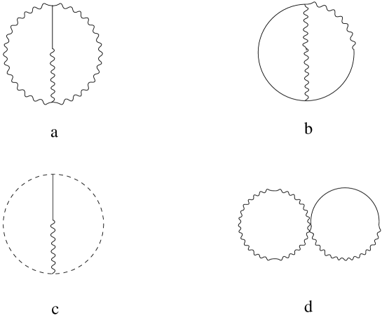
Figure 4: Two-loop diagrams with the mixings of the $h_{\mu\nu}$ and $\psi$ fields’ propagators

There are four types of the diagrams figs.4a-4d which give nontrivial contributions. Each of them has only single mixing of $h_{\mu\nu}$ and $\psi$ fields’ propagators. The diagrams with the double mixings or more are found to give no divergent contribution.

The evaluation of the diagrams with the mixings is much easier than that of the ones without the mixings, since there does not exist the parallel displacement matrix $a_{0}$ connecting $h_{\mu\nu}$ field to $\psi$ field. We have obtained only the non-local divergences for each of the diagrams. This is because the local divergences necessarily arise from the coincidence limit (2.59) of the $1$st Seeley coefficient $a_{1\ {\mu\nu},\psi^{\prime}}$ but it is a traceless matrix. As a result, we have found the sum of the amplitudes to be the following non-local divergences.

$${G\over 4\pi}\int d^{D}x\sqrt{\hat{g}}\ {2\sqrt{2}\over 3\epsilon}ai(\nabla_{\mu}\nabla_{\nu}\overline{G}{{}^{\mu\nu}{}_{,\psi}}|+\hat{R}_{\mu\nu}\overline{G}{{}^{\mu\nu}{}_{,\psi}}|)\ .$$ (3.18)

As it is expected they are just cancelled by the contribution from the counter terms (3.20).

3.5 Contributions from The One-loop Finite or One-loop Counter Terms

Finally, we evaluate the amplitudes for the diagrams with the insertion of the one-loop finite terms or the one-loop counter terms.

Figure 5: Two-loop diagrams with the insertion of one-loop finite terms

We have the only diagram fig.5 to consider for the contribution from the one-loop finite terms. The divergent part of the diagram is found from (2.32) to be

$${G\over(4\pi)^{2}}\int d^{D}x\sqrt{\hat{g}}\ {-25+c\over 6\epsilon}\hat{R}\ .$$ (3.19)

Figure 6: Two-loop diagrams with the insertion of one-loop counter terms

In a similar fashion, we can easily evaluate the diagrams with the insertion of the one-loop counter terms. We have obtained the sum of the divergent amplitudes for figs.6a and 6b from (2.21) and (2.34) as follows:

$${G\over(4\pi)^{2}}\int d^{D}x\sqrt{\hat{g}}\ {-95+3c\over 9\epsilon}\hat{R}$$ (3.20)

$$+ {G\over 4\pi}\int d^{D}x\sqrt{\hat{g}}\ \biggl{\{}-{33-c\over 12\epsilon}(\nabla^{2}\overline{G}_{{\mu\nu},}{}^{\mu\nu}|-2\nabla_{\mu}\nabla_{\nu}\overline{G}{{}^{\nu}{}_{\rho,}{}^{\mu\rho}}|+2\hat{R}_{\mu\rho\nu\sigma}\overline{G}{{}^{{\mu\nu},{\rho\sigma}}}|)$$

$$\qquad\qquad\qquad\ -{2\sqrt{2}\over 3\epsilon}ai(\nabla_{\mu}\nabla_{\nu}\overline{G}{{}^{\mu\nu}{}_{,\psi}}|+\hat{R}_{\mu\nu}\overline{G}{{}^{\mu\nu}{}_{,\psi}}|)$$

$$\qquad\qquad\qquad\ +{1\over 3\epsilon}(\nabla^{2}\overline{G}{{}^{\rm gh}{}_{\mu}{}^{\mu}}|-\hat{R}_{\mu\nu}\overline{G}{{}^{{\rm gh}\ \mu\nu}}|)\biggr{\}}\ .$$

3.6 Total Amplitude

After these calculations, the sum of the two loop divergences except those from the counter terms is evaluated by summing the contributions of (3.6), (3.11), (3.12), (3.13), (3.14), (3.15), (3.16), (3.17), (3.18) and (3.19) :

$${G\over(4\pi)^{2}}\int d^{D}x\sqrt{\hat{g}}\ {113+3c\over 72\epsilon}\hat{R}$$ (3.21)

$$+ {G\over 4\pi}\int d^{D}x\sqrt{\hat{g}}\ \biggl{\{}{33-c\over 12\epsilon}(\nabla^{2}\overline{G}_{{\mu\nu},}{}^{\mu\nu}|-2\nabla_{\mu}\nabla_{\nu}\overline{G}{{}^{\nu}{}_{\rho,}{}^{\mu\rho}}|+2\hat{R}_{\mu\rho\nu\sigma}\overline{G}{{}^{{\mu\nu},{\rho\sigma}}}|)$$

$$\qquad\qquad\qquad+{2\sqrt{2}\over 3\epsilon}ai(\nabla_{\mu}\nabla_{\nu}\overline{G}{{}^{\mu\nu}{}_{,\psi}}|+\hat{R}_{\mu\nu}\overline{G}{{}^{\mu\nu}{}_{,\psi}}|)$$

$$\qquad\qquad\qquad-{1\over 3\epsilon}(\nabla^{2}\overline{G}{{}^{\rm gh}{}_{\mu}{}^{\mu}}|-\hat{R}_{\mu\nu}\overline{G}{{}^{{\rm gh}\ \mu\nu}}|)$$

$$\qquad\qquad\qquad-{11\over 12\epsilon}(\hat{R}_{\mu\nu}-{1\over 2}\hat{g}_{\mu\nu}\hat{R})\ \overline{G}{{}^{\mu}{}_{\rho,}{}^{\nu\rho}}|\ \biggr{\}}\ .$$

Here, we note that the non-local divergences originate from the one-loop sub-divergences multiplied by the non-local parts of the propagators with possible derivatives $\overline{G},\nabla^{2}\overline{G},\nabla_{\mu}\nabla_{\nu}\overline{G}$. This is directly seen from our calculation procedure. When we evaluate a non-local divergence at the two-loop level, we replace one of the propagators of a two-loop diagram by its non-local part $\overline{G}$. A non-local divergence is just a non-local part $\overline{G}$ multiplied by a local divergence of a sub-loop which exist in the relevant diagram.

Therefore the non-local divergences at the two loop level exactly match the one-loop divergent corrections of quantum two-point functions. For example, let us consider a pair of the three-point vertices of quantum fields. We choose a pair of quantum fields from the each of the vertices as external fields. Next, we make a loop connecting the remaining two-point vertices. The one-loop divergent correction of a quantum two-point function is the two external fields multiplied by the local divergence of the loop. This is identical to a non-local divergence of a two-loop diagram, if we replace the two external fields by the non-local part of their propagator $\overline{G}$. Conversely we have the following transformation rules, which give a one-loop divergence for a quantum two-point function from a non-local divergence of a two-loop diagram. For example,

$${{\rm const.}\over\epsilon}\nabla_{\mu}\nabla_{\nu}\overline{G}{{}^{\nu}{}_{\rho,}{}^{\mu\rho}}| \longrightarrow -{{\rm const.}\over\epsilon}\nabla_{\mu}h^{\mu}{}_{\rho}\nabla_{\nu}h^{\nu\rho}\ ,$$

$${{\rm const.}\over\epsilon}\hat{R}_{\mu\rho\nu\sigma}\overline{G}{{}^{{\mu\nu},{\rho\sigma}}}| \longrightarrow {{\rm const.}\over\epsilon}\hat{R}_{\mu\rho\nu\sigma}h^{\mu\nu}h^{\rho\sigma}\ .$$ (3.22)

We can therefore determine the one-loop quantum field renormalizations which are required to cancel the nonlocal divergences of the two loop amplitudes if we evaluate the non-local parts of the two-loop corrections. The renormalizability of the theory implies that the necessary counter terms can be supplied by the renormalization of the couplings and the fields. On the other hand, we have already determined the counter terms (2.34) which consist of the one-loop renormalization of the gravitational coupling constant and the linear wave function renormalization of the quantum fields[13].

The sum of the amplitudes (3.21) and (3.20) are indeed found to be local except the term which is proportional to the field equation:

$${G\over(4\pi)^{2}}\int d^{D}x\sqrt{\hat{g}}\ {-79+3c\over 8\epsilon}\hat{R}$$ (3.23)

$$+ {G\over 4\pi}\int d^{D}x\sqrt{\hat{g}}\ \biggl{(}-{11\over 12\epsilon}\biggr{)}(\hat{R}_{\mu\nu}-{1\over 2}\hat{g}_{\mu\nu}\hat{R})\overline{G}{{}^{\mu}{}_{\rho,}{}^{\nu\rho}}|\ .$$

Since the field equations appear when we take the variation of the action by the fields, the remaining divergence can be dealt with by a nonlinear field renormalization at the one loop level. Previously we missed this counter term since we considered only the linear wave function renormalization of the fields. We remark that there is no principle to prohibit the nonlinear field renormalizations in this theory since the fields are dimensionless. Therefore, we are led to introduce the following renormalization of $h_{\mu\nu}$ field, paying attention to the traceless property.

$$h^{0}_{\mu\nu}=\biggl{(}1-{G\over 6\pi\epsilon}\biggr{)}h_{\mu\nu}\ +\ Z_{\rm n.l.}\biggl{(}h_{\mu\rho}h^{\rho}{}_{\nu}-{1\over D}\hat{g}_{\mu\nu}h_{\rho\sigma}h^{\rho\sigma}\biggr{)}\ .$$ (3.24)

From the linear terms of the expansion (2.26) we obtain additional counter terms, and find the expectation values of them to give only the non-local divergences:

$$\int d^{D}x\sqrt{\hat{g}}\ 2Z_{\rm n.l.}(\hat{R}_{\mu\nu}-{1\over 2}\hat{g}_{\mu\nu}\hat{R})\overline{G}{{}^{\mu}{}_{\rho,}{}^{\nu\rho}}|\ .$$ (3.25)

Therefore, the two-loop expectation value (3.23) can be made to be local, only if we choose the non-linear renormalization constant $Z_{\rm n.l.}$ of $h_{\mu\nu}$ field as

$$Z_{\rm n.l.}\ =\ {G\over 4\pi}{11\over 24\epsilon}\ .$$ (3.26)

Finally the total divergent contribution to the effective action at the two loop level in pure Einstein gravity is found to be of the renormalizable form.

$${G\over(4\pi)^{2}}\int d^{D}x\sqrt{\hat{g}}\ {-79+3c\over 8\epsilon}\hat{R}\ .$$ (3.27)

Here, we note that there arises only the single-pole divergence. The cancellation of the double-pole divergences is necessary for the consistency of the theory.

4 Renormalization of the Cosmological Constant Operator

In this section, we study the renormalization of the cosmological constant operator. As it will be shown, we need to introduce new counter terms to renormalize the cosmological constant operator. We also show that these new counter terms do not spoil the result of the previous section. We consider an infinitesimal perturbation of the theory by the cosmological constant operator by adding the following term to the action:

$$\Lambda\int d^{D}x\sqrt{g} = \Lambda\int d^{D}x\sqrt{\hat{g}}(1+{2\epsilon b\over a}\psi)^{2D\over\epsilon}$$ (4.1)

$$\simeq \Lambda\int d^{D}x\sqrt{\hat{g}}\exp\bigl{(}(1-{\epsilon\over 2}){1\over a}\psi-{\epsilon\over 8a^{2}}\psi^{2}+\ldots\bigr{)}\ .$$

This term is manifestly generally covariant and it is invariant under the gauge transformation (2.30). The quadratic part of the action with respect to $\psi$ field becomes:

$$\int d^{D}x\sqrt{\hat{g}}\biggl{(}-{\mu^{\epsilon}\over 2G}(1-a^{2})\partial_{\mu}\psi\partial^{\mu}\psi+\Lambda\mu^{D}(1-{5\epsilon\over 4}){1\over 2a^{2}}\psi^{2}+{1\over G}\epsilon b\hat{R}\psi^{2}\biggr{)}\ .$$ (4.2)

We regard $\Lambda$ to be infinitesimally small and evaluate the divergent part of the effective action proportional to $\Lambda$. Namely we consider the diagrams with the single insertion of the cosmological constant operator. Further insertions of the cosmological constant operator do not lead to the short distance divergences by the power counting. We utilize the same covariant calculation method which has been employed in the previous section. The relevant diagrams in this section are those which contain $\psi$ field propagators. The divergent part proportional to $\Lambda$ at the one loop level is

$$-\int d^{D}x\sqrt{\hat{g}}({G\over{4\pi}})\Lambda({1\over\epsilon a^{2}}+{1\over\epsilon})\ .$$ (4.3)

At the two loop level, we find the following divergences:

$$\int d^{D}x\sqrt{\hat{g}}\biggl{(}({G\over{4\pi}})^{2}\Lambda\bigl{(}({1\over{\epsilon a^{2}}})({-1\over 4})+{-3\over\epsilon^{2}}+({1\over\epsilon})({-35\over 8}+4\pi\bar{G}_{\mu\nu},^{\mu\nu})\bigr{)}+{G\over{4\pi\epsilon}}a^{2}\nabla^{2}\bar{G}_{\psi\psi}|\biggr{)}\ .$$ (4.4)

Here we omit the square of the one loop result (4.3). In this expression, we find two types of the nonlocal divergences.

The first type arises due to the one loop level divergence of ${G\over{4\pi\epsilon}}\Lambda\int d^{D}x\sqrt{\hat{g}}h_{\mu\nu}h^{\mu\nu}$ form. It also leads to the double pole singularity in (4.4). Such a divergence can be subtracted by the nonlinear wave function renormalization of $\psi$ field as $\psi^{0}=\psi+a({G\over{4\pi\epsilon}})(h_{\mu\nu}h^{\mu\nu}+{G\over\pi\epsilon})$. The last term at $O(G^{2})$ is added in order to cancel the leading singularity of the vacuum expectation value of $\psi$. By doing so, we can eliminate the first nonlocal divergence in (4.4) and obtain

$$\int d^{D}x\sqrt{\hat{g}}\biggl{(}({G\over{4\pi}})^{2}\Lambda\bigl{(}({1\over{\epsilon a^{2}}})({-1\over 4})+{-3\over\epsilon^{2}}+({1\over\epsilon})({-27\over 8})\bigr{)}+{G\over{4\pi\epsilon}}a^{2}\nabla^{2}\bar{G}_{\psi\psi}|\biggr{)}\ .$$ (4.5)

This procedure also gives rise to the following counter term from the Einstein action:

$$({a^{2}\over 4\pi\epsilon})\int d^{D}x\sqrt{\hat{g}}\hat{R}(h_{\mu\nu}h^{\mu\nu}+{G\over\pi\epsilon})\ .$$ (4.6)

At the one loop level, it can be regarded to be a finite counter term by expanding $a^{2}$ in terms of $G$. It leads to no new divergence of $\int d^{D}x\sqrt{\hat{g}}\hat{R}$ type at the two loop level. Therefore this new counter term is harmless to the order in the perturbation theory we are working here.

We have also found the following contribution of the $\psi$ field kinetic term type due to the one loop subloops of $h_{\mu\nu}$ and ghost fields which is responsible for the second nonlocal divergence in (4.4):

$$-({a^{2}\over 4\pi\epsilon})\int d^{D}x\sqrt{\hat{g}}\partial_{\mu}\psi\partial^{\mu}\psi\ .$$ (4.7)

This one loop contribution is another source of the double pole singularity of the cosmological constant operator at the two loop level. It is because $a^{2}$ factor in the numerator of this term can be cancelled by the inverse power of $a$ which is associated with $\psi$ field in the cosmological constant operator. We need to subtract this term from the one loop subdiagrams when we consider the diagrams with the single insertion of the cosmological constant operator. In order to do so, we have chosen to adopt the following counter term in the action:

$$({(D-1)a^{2}\over 2\pi\epsilon})\int d^{D}x\sqrt{\hat{g}}\biggl{(}\tilde{R}(1+a\psi+\epsilon b\psi^{2})-{1\over 2}\partial_{\mu}\psi\partial^{\mu}\psi\biggr{)}\ .$$ (4.8)

This action contains the desired counter term of the $\psi$ field kinetic term type. Although it contains other counter terms, they can be regarded as finite counter terms by expanding $a^{2}$ in terms of $G$. It is because $\psi$ field appears with additional factors of $a$ or $\epsilon$ as long as they are concerned. The terms which involve only $h_{\mu\nu}$ field are safe since they do not couple to $\psi$ field directory. After this procedure, the two loop level divergence proportinal to $\Lambda$ becomes:

$$\int d^{D}x\sqrt{\hat{g}}({G\over{4\pi}})^{2}\Lambda\biggl{(}({1\over{\epsilon a^{2}}})({-1\over 4})+{-1\over\epsilon^{2}}+({1\over\epsilon})({-7\over 8})\biggr{)}\ .$$ (4.9)

The counter terms (4.8) do not give rise to new divergences of the Einstein action form neither at the two loop level.

After these considerations, we find that the divergence of the effective action which is proportinal to $\Lambda$ is local. However it still contains the double pole in $\epsilon$. The double pole here can be removed by the following wave function renormalization. We note that there is a freedom of the scale transformation of the background metric. We utilize this freedom to eliminate the divergences of the cosmological constant type which is independent of $a^{2}$. We rescale the background metric by the following factor:

$$Z=1+({G\over{4\pi}})^{2}({-1\over\epsilon^{2}})\ .$$ (4.10)

After the scaling, the remaining two loop level divergence proportinal to $\Lambda$ has only the simple pole in $\epsilon$:

$$\int d^{D}x\sqrt{\hat{g}}({G\over{4\pi}})^{2}\Lambda\biggl{(}({1\over{\epsilon a^{2}}})({-1\over 4})+({1\over\epsilon})({-7\over 8})\biggr{)}\ .$$ (4.11)

This procedure also leads to the rescaling of the Einstein action.

$$Z^{{\epsilon\over 2}}\int d^{D}x\sqrt{\hat{g}}{1\over G}\hat{R}\ ,$$

$$Z^{{\epsilon\over 2}}\ =\ 1+\biggl{(}{G\over 4\pi}\biggr{)}^{2}({-1\over 2\epsilon})\ .$$ (4.12)

Here, the exponent: ${\epsilon\over 2}$ is seen from the dependence of the Einstein term and the cosmological constant operator on the conformal mode.

$$\sqrt{g}R\simeq e^{-{\epsilon\over 2}\phi}\sqrt{\hat{g}}\tilde{R}\ \ ,\ \ \sqrt{g}\simeq e^{-{D\over 2}\phi}\sqrt{\hat{g}}\ .$$ (4.13)

The rescaling of the background metric introduces a new counter term as in (4.12). Due to the new counter term, the total two-loop divergence of the effective action which is of the Einstein action type becomes the following instead of the final result of the previous section (3.27):

$${G\over(4\pi)^{2}}\int d^{D}x\sqrt{\hat{g}}\ {-3(25-c)\over 8\epsilon}\hat{R}\ .$$ (4.14)

It has a simple pole in $\epsilon$ and vanishes when $c=25$ which corresponds to the critical string theory in the two dimensional limit. These are certainly the desirable features.

Here we recall the counter terms at the one loop level which can be associated with the bare gravitational coupling constant

$$-{\mu^{\epsilon}\over G}({25-c\over 6\epsilon})({G\over 4\pi})+{(D-1)a^{2}\over 2\pi\epsilon},$$ (4.15)

$$= -{\mu^{\epsilon}\over G}({25-c\over 6\epsilon})({G\over 4\pi})+{\mu^{\epsilon}\over 4\pi}\biggl{(}1-({25-c\over 6\epsilon})({G\over 4\pi})\biggr{)}$$

The first term is the coefficient of $\int d^{D}x\sqrt{\hat{g}}\tilde{R}$ and the second term is the coefficient of the Einstein action in (4.8). The only first term contributes to the conformal anomaly at the one loop level and enters in the definition of $a^{2}$ at $O(G)$[16]. We note that the second term contains $O(G)$ term. We have to add an appropriate $O(G)$ term to it in order to cancel (4.14).

In this way, the bare gravitational coupling constant at the two loop level is found to be

$${1\over G^{0}}={\mu^{\epsilon}\over G}(1+{G\over 4\pi})\biggl{(}1-({25-c\over 6\epsilon})({G\over 4\pi})-({5(25-c)\over 24\epsilon})({G\over 4\pi})^{2}\biggr{)}$$ (4.16)

We can still remove the factor $(1+{G\over 4\pi})$ from this quantity by rescaling the background metric. We also need to multiply the factor $(1+{G\over 4\pi})^{-2\over\epsilon}$ to the cosmological constant operator at the same time. In such a renormalization scheme, the bare gravitational coupling constant is found to be:

$${1\over G^{0}}={\mu^{\epsilon}\over G}\biggl{(}1-({25-c\over 6\epsilon})({G\over 4\pi})-({5(25-c)\over 24\epsilon})({G\over 4\pi})^{2}\biggr{)}$$ (4.17)

The $\beta$ function of the gravitational coupling constant is

$$\beta_{G}=\epsilon G-({25-c\over 6})({G\over 4\pi})G-({5(25-c)\over 12})({G\over 4\pi})^{2}G$$ (4.18)

It agrees with our previous result of [14] to the leading order in $c$.

The remaining simple pole divergences of the cosmological constant operator which are inversely proportional to $a^{2}$ can be ascribed to the singular expectation value of $\psi^{2}$:

$$<\psi^{2}>={G\over 2\pi\epsilon}\biggl{(}1+({1\over 4}){G\over 4\pi}\biggr{)}$$ (4.19)

They are of order $(G/a^{2})$ and they can become large around the short distance fixed point of the renormalization group where $a^{2}\rightarrow 0$. At higher orders, we also find the divergences of order $(G/a^{2})^{n}$. Therefore we need to sum this class of contributions to all orders. It can be done by considering the following integral[11].

$$\int d\psi exp\biggl{(}{4\over\epsilon}log(1+{\epsilon\psi\over 4a})-{\pi\epsilon\over G}(1-({1\over 4}){G\over 4\pi})\psi^{2}\biggr{)}$$ (4.20)

This integral can be evaluated for small $\epsilon$ by the saddle point method with the change of the variables: ${\epsilon\psi\over 4a}=\rho$. The saddle point of $\rho$ satisfies:

$$\rho_{0}(1+\rho_{0})-{G\over 8\pi a^{2}}\biggl{(}1+({1\over 4}){G\over 4\pi}\biggr{)}=0$$ (4.21)

The renormalization factor is found to be

$$Z_{\Lambda}=exp\biggl{(}{4\over\epsilon}log(1+\rho_{0})-{16\pi a^{2}\over\epsilon G}(1-{G\over 16\pi})\rho_{0}^{2}\biggr{)}exp(-{G\over 4\pi\epsilon})$$ (4.22)

where the last factor is necessary to cancel the one loop divergence which is independent of $a^{2}$. The anomalous dimension is found to be

$$\gamma = \mu{\partial\over\partial\mu}logZ_{\Lambda},$$ (4.23)

$$= {16\pi a^{2}\over G}\rho_{0}^{2}-{G\over 4\pi}$$

We therefore find the anomalous dimension to be

$$2(1-{G\over 16\pi})-{8\pi\over G}\biggl{(}-a^{2}+\sqrt{a^{4}+{Ga^{2}\over 2\pi}(1+{G\over 16\pi})}\biggr{)}$$ (4.24)

In these considerations, $a^{2}$ is regarded as $O(G)$ quantity and the anomalous dimension is $O(1)$ at the one loop level. At the two loop level, we find a finite correction of $O(G)$ to the leading result.

At the short distance fixed point of the renormalization group where $a^{2}$ vanishes, we find the anomalous dimension of the cosmological constant operator to be

$$2(1-{G^{*}\over 16\pi})$$ (4.25)

where $G^{*}={24\pi\epsilon\over 25-c}+O(\epsilon^{2})$ is the fixed point coupling constant. The scaling dimension is the sum of the canonical and the anomalous dimensions. The scaling dimension of the cosmological constant operator around the fixed point is found to be

$$-(2+\epsilon)+2-{G^{*}\over 8\pi}=-\epsilon-{3\epsilon\over 25-c}+O(\epsilon^{2})$$ (4.26)

The leading order quantity of $O(1)$ has been cancelled by the quantum correction and the scaling dimension is found to be $O(\epsilon)$ by the two loop level calculation.

The scaling dimension of the inverse gravitational coupling constant around the fixed point is:

$$\mu{\partial\over\partial\mu}({1\over G}-{1\over G^{*}})=-\epsilon({1\over G}-{1\over G^{*}})+O(\epsilon^{2})$$ (4.27)

Since the scaling dimension of the cosmological constant operator is determined to be $O(\epsilon)$ by the two loop calculation, we only need the one loop $\beta$ function of the gravitational coupling constant here. It is because of the cancelation of the leading $O(1)$ term in the scaling dimension of the cosmological constant operator. In order to determine the scaling dimension up to $O(\epsilon^{2})$, we need to renormalize the cosmological constant operator up to higher orders. We find that the both gravitational and the cosmological couplings are relevant. Although they are also relevant couplings classically, the scaling dimension of the cosmological constant operators has changed drastically from the classical value of $D$ to that of $O(\epsilon)$. However these scaling dimensions separately cannot be physical quantities. It is because they are scheme dependent on how we rescale the metric.

The physically meaningful prediction is the scaling relation between the gravitational coupling constant and the cosmological constant. We find the scaling relation between the gravitational coupling constant and the cosmological constant at the short distance fixed point as

$$({1\over G}-{1\over G^{*}})^{\epsilon+{3\epsilon\over 25-c}}\sim\Lambda^{\epsilon}$$ (4.28)

It is very different from the classical scaling relation which holds at the weak coupling infrared fixed point:

$$({1\over G})^{D}\sim\Lambda^{\epsilon}$$ (4.29)

These scaling exponents have been numerically measured in four dimensions by using a real space renormalization group technique[17]. What has been observed is the following scaling relation at an ultraviolet stable fixed point:

$$N^{-{\beta_{0}\over 4}}\sim|\kappa^{*}-\kappa|$$ (4.30)

where $\kappa$ is the inverse gravitational coupling constant and $N$ is the space time volume which is dual to the cosmological constant. Therefore it leads

$$\Lambda^{{\beta_{0}\over 4}}\sim|\kappa^{*}-\kappa|$$ (4.31)

$\beta_{0}$ is measured to be $6.5(1.2)$. If we put $\epsilon=2$ in our scaling relation (4.28), it gives $\beta_{0}\sim 4$. On the other hand, the classical scaling relation corresponds to the exponent $\beta_{0}=2$. We observe that our prediction is closer to the measured value than the classical exponent.

5 Conclusions and Discussions

In this paper, we have performed the two loop level renormalization of the quantum gravity in $2+\epsilon$ dimensions. We have adopted the background gauge and computed the effective action of the background fields which is manifestly covariant. We have made the most of the covariance to simplify the calculation. We have shown that the short distance divergences are renormalizable within our scheme to the two loop level.

In fact we have explicitly determined the counter terms which make the effective action finite up to this order. These counter terms are all of the expected types which can be supplied by the renormalization of the couplings and the wave functions. The most nontrivial counter term is the type of $\int d^{D}x\sqrt{\hat{g}}\tilde{R}$ which gives rise to the conformal anomaly. Our renormalization scheme is successful to handle it by choosing the “linear dilaton” type coupling $a$ in such a way to maintain the conformal invariance with respect to the background metric. The bare action can be chosen to be a manifestly covariant form simultaneously[16]. We have thus demonstrated the effectiveness of our formalism by the explicit calculations reported here.

We have further predicted the scaling relations and the scaling exponents between the gravitational and the cosmological coupling constants. Such a prediction can be compared with recent numerical investigations in quantum gravity. We have found that our prediction appears to be closer to the measured value than the classical prediction. However it also turns out that taking the continuum limit is not straightforward at the ultraviolet stable fixed point where the scaling is observed[18]. The problem is that the phase transition appears to be of the first order rather than the second order. So constructing a realistic quantum gravity theory still is a challenging task and the exponent which has been measured in the numerical approach may be taken qualitatively at best.

However we cannot rule out the possibility that the continuum limit may be taken with further ingenuity and the scaling behavior currently observed may qualitatively survive. Therefore we believe that it is worthwhile to seriously attempt to calculate the scaling exponents in the continuum approach in view of the progress which has been already achieved in the numerical approach. We hope that our results will shed light on the continuum quantum gravity with such an optimism.

Appendix A Singular Products of The Functions $G_{0},G_{1}$

In the course of the calculation of the two-loop amplitudes, we need to know the singular behavior of the several products of the functions $G_{0}$’s and $G_{1}$’s at short distance. In general, the singular part is given by the bi-scalar delta functions with derivatives or those multiplied by covariant curvature tensors. In terms of them, we can evaluate the loop amplitudes in a manifestly covariant way. In this appendix, we will illustrate the derivation of them [23] .

The functions $G_{0}$ and $G_{1}$ are effectively defined by the equations (2.18). The consistency with the first of (2.18) and the coincidence limits (2.19) lead us to find the singular behavior:

$$\nabla_{\mu}\nabla_{\nu}G_{0}\cdot G_{0}{}^{n}\sim-{(-1)^{n}\over D}{\mu^{n\epsilon}\over(2\pi\epsilon)^{n}}\ \hat{g}_{\mu\nu}\delta^{D}\ ,$$ (A.1)

from which we can immediately obtain, discarding a non-singular total derivative,

$$\nabla_{\mu}G_{0}\nabla_{\nu}G_{0}\cdot G_{0}{}^{n-1}\sim{1\over D}{(-1)^{n}\over n}{\mu^{n\epsilon}\over(2\pi\epsilon)^{n}}\ \hat{g}_{\mu\nu}\delta^{D}\ .$$ (A.2)

Differentiating (A.1) and (A.2), we can derive the singular behavior of the products with three derivatives. They are proportional to the delta functions with a derivative, since there does not exist a covariant curvature term of the mass dimension one.

$$\nabla_{\mu}\nabla_{\nu}G_{0}\nabla_{\rho}G_{0}\cdot G_{0}{}^{n-1}$$

$$\sim -{1\over D+2}{(-1)^{n}\over n}{\mu^{n\epsilon}\over(2\pi\epsilon)^{n}}\biggl{(}{2\over D}\hat{g}_{\mu\nu}\partial_{\rho}-\hat{g}_{\mu\rho}\partial_{\nu}-\hat{g}_{\nu\rho}\partial_{\mu}\biggr{)}\delta^{D}\ ,$$

$$\nabla_{\mu}G_{0}\nabla_{\nu}G_{0}\nabla_{\rho}G_{0}\cdot G_{0}{}^{n-2}$$

$$\sim -{\epsilon\over D(D+2)}{(-1)^{n}\over n(n-1)}{\mu^{n\epsilon}\over(2\pi\epsilon)^{n}}(\hat{g}_{\mu\nu}\partial_{\rho}+\hat{g}_{\mu\rho}\partial_{\nu}+\hat{g}_{\nu\rho}\partial_{\mu})\delta^{D}\ .$$ (A.4)

Here, we have used the result.

$$\nabla_{\mu}\nabla_{\nu}\nabla_{\rho}G_{0}\cdot G_{0}{}^{n}$$ (A.5)

$$\sim -{(-1)^{n}\over D+2}{\mu^{n\epsilon}\over(2\pi\epsilon)^{n}}(\hat{g}_{\mu\nu}\partial_{\rho}+\hat{g}_{\mu\rho}\partial_{\nu}+\hat{g}_{\nu\rho}\partial_{\mu})\delta^{D}\ ,$$

which is obtained, in the same way as (A.1), from the symmetry under the exchange of the indices of the singular part.

Next, we proceed to the singular behavior of the products of the functions $G_{0}$’s and $G_{1}$’s with four derivatives. They have the mass dimension four. So, the singular piece consists of the bi-scalar delta functions with the quadratic derivatives or those multiplied by the curvature tensors.

We cite the results for the singular parts of the products of $G_{0}$’s and $G_{1}$’s.

$$\nabla_{\mu}\nabla_{\nu}G_{0}\nabla_{\rho}\nabla_{\sigma}G_{0}\cdot G_{0}{}^{n-1}$$

$$\sim {1\over(D+2)(D+4)}{(-1)^{n}\over n}{\mu^{n\epsilon}\over(2\pi\epsilon)^{n}}\biggl{\{}{2-\epsilon\over D}\hat{g}_{\mu\nu}\hat{g}_{\rho\sigma}\nabla^{2}\delta^{D}+{D\over 2}(\hat{g}_{\mu\rho}\hat{g}_{\nu\sigma}+\hat{g}_{\mu\sigma}\hat{g}_{\nu\rho})\nabla^{2}\delta^{D}$$

$$- 4(\hat{g}_{\mu\nu}\nabla_{\rho}\nabla_{\sigma}+\hat{g}_{\rho\sigma}\nabla_{\mu}\nabla_{\nu})\delta^{D}$$

$$+ D(\hat{g}_{\mu\rho}\nabla_{\nu}\nabla_{\sigma}+\hat{g}_{\mu\sigma}\nabla_{\nu}\nabla_{\rho}+\hat{g}_{\nu\rho}\nabla_{\mu}\nabla_{\sigma}+\hat{g}_{\nu\sigma}\nabla_{\mu}\nabla_{\rho})\delta^{D}\biggr{\}}$$

$$+ {1\over 3(D+2)}{(-1)^{n}\over n}{\mu^{n\epsilon}\over(2\pi\epsilon)^{n}}\{2(\hat{R}_{\mu\rho\nu\sigma}+\hat{R}_{\mu\sigma\nu\rho})$$

$$+ (\hat{g}_{\mu\rho}\hat{R}_{\nu\sigma}+\hat{g}_{\mu\sigma}\hat{R}_{\nu\rho}+\hat{g}_{\nu\rho}\hat{R}_{\mu\sigma}+\hat{g}_{\nu\sigma}\hat{R}_{\mu\rho})\}\delta^{D}$$

$$- {1\over 6(D+2)(D+4)}{(-1)^{n}(n-1)\over n}{\mu^{n\epsilon}\over(2\pi\epsilon)^{n}}\biggl{\{}\biggl{(}1-{2\epsilon\over D}\biggr{)}\hat{g}_{\mu\nu}\hat{g}_{\rho\sigma}\hat{R}$$

$$+ {D\over 2}(\hat{g}_{\mu\rho}\hat{g}_{\nu\sigma}+\hat{g}_{\mu\sigma}\hat{g}_{\nu\rho})\hat{R}-4(\hat{g}_{\mu\nu}\hat{R}_{\rho\sigma}+\hat{g}_{\rho\sigma}\hat{R}_{\mu\nu})$$

$$+ D(\hat{g}_{\mu\rho}\hat{R}_{\nu\sigma}+\hat{g}_{\mu\sigma}\hat{R}_{\nu\rho}+\hat{g}_{\nu\rho}\hat{R}_{\mu\sigma}+\hat{g}_{\nu\sigma}\hat{R}_{\mu\rho})\biggr{\}}\delta^{D}$$

$$+ {(-1)^{n}\over 6D}{\mu^{n\epsilon}\over(2\pi\epsilon)^{n}}(\hat{g}_{\mu\nu}\hat{R}_{\rho\sigma}+\hat{g}_{\rho\sigma}\hat{R}_{\mu\nu})\delta^{D}\ ,$$

$$\nabla_{\mu}\nabla_{\nu}G_{0}\nabla_{\rho}G_{0}\nabla_{\sigma}G_{0}\cdot G_{0}{}^{n-2}$$

$$\sim {\epsilon\over(D+2)(D+4)}{(-1)^{n}\over n(n-1)}{\mu^{n\epsilon}\over(2\pi\epsilon)^{n}}\biggl{\{}{2\over D}\hat{g}_{\mu\nu}\hat{g}_{\rho\sigma}\nabla^{2}\delta^{D}-{1\over 2}(\hat{g}_{\mu\rho}\hat{g}_{\nu\sigma}+\hat{g}_{\mu\sigma}\hat{g}_{\nu\rho})\nabla^{2}\delta^{D}$$

$$+ {4\over D}\hat{g}_{\mu\nu}\nabla_{\rho}\nabla_{\sigma}\delta^{D}-\hat{g}_{\rho\sigma}\nabla_{\mu}\nabla_{\nu}\delta^{D}$$

$$- (\hat{g}_{\mu\rho}\nabla_{\nu}\nabla_{\sigma}+\hat{g}_{\mu\sigma}\nabla_{\nu}\nabla_{\rho}+\hat{g}_{\nu\rho}\nabla_{\mu}\nabla_{\sigma}+\hat{g}_{\nu\sigma}\nabla_{\mu}\nabla_{\rho})\delta^{D}\biggr{\}}$$

$$- {\epsilon\over 3D(D+2)}{(-1)^{n}\over n(n-1)}{\mu^{n\epsilon}\over(2\pi\epsilon)^{n}}\{2(\hat{R}_{\mu\rho\nu\sigma}+\hat{R}_{\mu\sigma\nu\rho})$$

$$+ (\hat{g}_{\mu\rho}\hat{R}_{\nu\sigma}+\hat{g}_{\mu\sigma}\hat{R}_{\nu\rho}+\hat{g}_{\nu\rho}\hat{R}_{\mu\sigma}+\hat{g}_{\nu\sigma}\hat{R}_{\mu\rho})\}\delta^{D}$$

$$+ {\epsilon\over 6(D+2)(D+4)}{(-1)^{n}\over n}{\mu^{n\epsilon}\over(2\pi\epsilon)^{n}}\biggl{\{}-{2\over D}\hat{g}_{\mu\nu}\hat{g}_{\rho\sigma}\hat{R}$$

$$+ {1\over 2}(\hat{g}_{\mu\rho}\hat{g}_{\nu\sigma}+\hat{g}_{\mu\sigma}\hat{g}_{\nu\rho})\hat{R}+(\hat{g}_{\mu\nu}\hat{R}_{\rho\sigma}+\hat{g}_{\rho\sigma}\hat{R}_{\mu\nu})$$

$$- {D\over 4}(\hat{g}_{\mu\rho}\hat{R}_{\nu\sigma}+\hat{g}_{\mu\sigma}\hat{R}_{\nu\rho}+\hat{g}_{\nu\rho}\hat{R}_{\mu\sigma}+\hat{g}_{\nu\sigma}\hat{R}_{\mu\rho})\biggr{\}}\delta^{D}$$

$$- {(-1)^{n}\over 6n}{\mu^{n\epsilon}\over(2\pi\epsilon)^{n}}\biggl{\{}{1\over D}(\hat{g}_{\mu\nu}\hat{R}_{\rho\sigma}+\hat{g}_{\rho\sigma}\hat{R}_{\mu\nu})$$

$$- {1\over 4}(\hat{g}_{\mu\rho}\hat{R}_{\nu\sigma}+\hat{g}_{\mu\sigma}\hat{R}_{\nu\rho}+\hat{g}_{\nu\rho}\hat{R}_{\mu\sigma}+\hat{g}_{\nu\sigma}\hat{R}_{\mu\rho})\biggr{\}}\delta^{D}\ .$$ (A.7)

These correspond to the overlapping divergences, when a part of the $x$ derivatives of $G_{0}$’s is converted into those with respect to $y$.

We also have to consider the products involving a function $G_{1}$. The equations (2.18) make it possible for us to reduce the derivative of $G_{1}$ to the sum of $G_{0}$’s and $G_{1}$’s with no derivative. Using them, we find the singular parts of the products including a function $G_{1}$ and four derivatives to be proportional to the delta functions without any derivatives or curvature tensors. There are three types of products necessary for our calculation.

$$\nabla_{\mu}\nabla_{\nu}G_{0}\nabla_{\rho}\nabla_{\sigma}G_{1}\cdot G_{0}{}^{n-1}$$

$$\sim {(-1)^{n}\over 2D}{\mu^{n\epsilon}\over(2\pi\epsilon)^{n}}\hat{g}_{\mu\nu}\hat{g}_{\rho\sigma}\delta^{D}$$

$$+ {1\over 2(D+2)}{(-1)^{n}\over n}{\mu^{n\epsilon}\over(2\pi\epsilon)^{n}}\biggl{(}-{2\over D}\hat{g}_{\mu\nu}\hat{g}_{\rho\sigma}+\hat{g}_{\mu\rho}\hat{g}_{\nu\sigma}+\hat{g}_{\mu\sigma}\hat{g}_{\nu\rho}\biggr{)}\delta^{D}\ ,$$

$$\nabla_{\mu}G_{0}\nabla_{\nu}G_{0}\nabla_{\rho}\nabla_{\sigma}G_{1}$$

$$\sim -{1\over 4D}{\mu^{2\epsilon}\over(2\pi\epsilon)^{2}}\hat{g}_{\mu\nu}\hat{g}_{\rho\sigma}\delta^{D}$$

$$- {\epsilon\over 4D(D+2)}{\mu^{2\epsilon}\over(2\pi\epsilon)^{2}}(\hat{g}_{\mu\nu}\hat{g}_{\rho\sigma}+\hat{g}_{\mu\rho}\hat{g}_{\nu\sigma}+\hat{g}_{\mu\sigma}\hat{g}_{\nu\rho})\delta^{D}\ ,$$

$$\nabla_{\mu}\nabla_{\nu}G_{0}\nabla_{\rho}G_{0}\nabla_{\sigma}G_{1}$$

$$\sim -{1\over 4(D+2)}{\mu^{2\epsilon}\over(2\pi\epsilon)^{2}}\biggl{(}{2\over D}\hat{g}_{\mu\nu}\hat{g}_{\rho\sigma}-\hat{g}_{\mu\rho}\hat{g}_{\nu\sigma}-\hat{g}_{\mu\sigma}\hat{g}_{\nu\rho}\biggr{)}\delta^{D}\ .$$ (A.10)

So far, we have considered the singular behavior of the products of $G_{0}$’s or $G_{1}$’s with only $x$ derivatives. Now, let us extend the previous results to the products with $x^{\prime}$ derivatives as well as those with respect to $x$.

We can convert the $x$ derivative of the functions $G_{0},G_{1}$ to that with respect to $x^{\prime}$, using an identity which uses the parallel displacement bi-vector $\gamma_{\mu}{}^{\nu^{\prime}}$:

$$\gamma_{\mu^{\prime}}{}^{\mu}\nabla_{\mu}G_{i}\ =\ -G_{i}{\overleftarrow{\nabla}}_{\mu^{\prime}}\ ,\ \ \ i=0,1.$$ (A.11)

As a result, the singular expansions (A.1)-(A.5) and (A)-(A.10) are valid under the change:

$$\nabla_{\mu}G_{i}\ \longrightarrow-\gamma_{\mu}{}^{\mu^{\prime}}G_{i}{\overleftarrow{\nabla}}_{\mu^{\prime}}\ ,\ \ \ i=0,1.$$ (A.12)

On the other hand, we should pay attention to the singular parts proportional to the quadratic derivatives of a delta function. In (A) and (A.7), we need additional curvature terms as

$$\gamma_{\rho}{}^{\rho^{\prime}}\nabla_{\mu}G_{0}{\overleftarrow{\nabla}}_{\rho^{\prime}}\cdot\gamma_{\sigma}{}^{\sigma^{\prime}}\nabla_{\nu}G_{0}{\overleftarrow{\nabla}}_{\sigma^{\prime}}\cdot G_{0}{}^{n-1}$$

$$\sim \nabla_{\mu}\nabla_{\rho}G_{0}\nabla_{\nu}\nabla_{\sigma}G_{0}\cdot G_{0}{}^{n-1}$$

$$- {1\over D+2}{(-1)^{n}\over n}{\mu^{n\epsilon}\over(2\pi\epsilon)^{n}}\biggl{\{}{1\over D}(\hat{g}_{\mu\rho}\hat{R}_{\nu\sigma}+\hat{g}_{\nu\sigma}\hat{R}_{\mu\rho})+\hat{R}_{{\mu\nu}{\rho\sigma}}+\hat{R}_{\mu\sigma\rho\nu}\biggr{\}}\delta^{D}\ ,$$

$$\gamma_{\rho}{}^{\rho^{\prime}}\nabla_{\mu}G_{0}{\overleftarrow{\nabla}}_{\rho^{\prime}}\cdot\nabla_{\nu}G_{0}\cdot\gamma_{\sigma}{}^{\sigma^{\prime}}G_{0}{\overleftarrow{\nabla}}_{\sigma^{\prime}}\cdot G_{0}{}^{n-2}$$

$$\sim \nabla_{\mu}\nabla_{\rho}G_{0}\nabla_{\nu}G_{0}\nabla_{\sigma}G_{0}\cdot G_{0}{}^{n-2}$$

$$+ {\epsilon\over 2D(D+2)}{(-1)^{n}\over n(n-1)}{\mu^{n\epsilon}\over(2\pi\epsilon)^{n}}(\hat{R}_{{\mu\nu}{\rho\sigma}}+\hat{R}_{\mu\sigma\rho\nu}-\hat{g}_{\nu\sigma}\hat{R}_{\mu\rho})\delta^{D}\ .$$ (A.14)

Here, we have used the coincidence limits (2.22).

References

• [1] G. ’t Hooft and M. Veltman, Ann. Inst. Henri Poincare 20 (1974) 69.
• [2] S. Weinberg, in General Relativity, an Einstein Centenary Survey,
eds. S.W. Hawking and W. Israel (Cambridge Univ. Press, 1979).
• [3] R. Gastmans, R. Kallosh and C. Truffin, Nucl. Phys. B133 (1978) 417.
• [4] S.M. Christensen and M.J. Duff, Phys. Lett. B79 (1978) 213.
• [5] H. Kawai and M. Ninomiya, Nucl. Phys. B336 (1990) 115.
• [6] V.G. Knizhnik, A.M. Polyakov and A.A. Zamolochikov,
Mod. Phys. Lett.A3 (1988) 819.
• [7] F. David, Mod. Phys. Lett. A3 (1988) 1651.
• [8] J. Distler and H. Kawai, Nucl. Phys. B321 (1989) 504.
• [9] C.G. Callan, D.H. Friedan, E.J. Martinec and M.J. Perry, Nucl. Phys. B262 (1985) 593.
• [10] E.S. Fradkin and A.A. Tseytlin, Nucl. Phys. B261 (1985) 1.
• [11] H. Kawai, Y. Kitazawa and M. Ninomiya, Nucl. Phys. B393 (1993) 280.
• [12] H. Kawai, Y. Kitazawa and M. Ninomiya, Nucl. Phys. B404 (1993) 684.
• [13] T. Aida, Y. Kitazawa, H. Kawai and M. Ninomiya, Nucl. Phys. B427 (1994) 158.
• [14] T. Aida, Y. Kitazawa, J. Nishimura and A. Tsuchiya, Nucl. Phys. B444 (1995) 353.
• [15] Y. Kitazawa, Nucl. Phys. B453 (1995) 477.
• [16] H. Kawai, Y. Kitazawa and M. Ninomiya, Nucl. Phys. B467 (1996) 313.
• [17] Z. Burda, J.-P. Kownacki and A. Krzywicki, Phys. Lett. B356 (1995) 466.
• [18] P. Bialas, Z. Burda, A. Krzywicki and B. Petersson, ”Focusing on the fixed point of 4-D simplical gravity”, heplat/9601024.
• [19] B.S. DeWitt, Dynamical theory of groups and fields (Gordon and Breach, 1965)
• [20] See for example, A. Barvinsky and G. Vilkovisky, Phys. Rep. 119 (1985) 1.
• [21] I. Jack and H. Osborn, Nucl. Phys. B207 (1982) 474.
• [22] I. Jack and H. Osborn, Nucl. Phys. B234 (1984) 331.
• [23] H. Osborn, Ann. Phys. 200 (1990) 1.