UCSBTH-96-22
Since the seminal work of Seiberg and Witten [1] we know that the exact quantum moduli space of $N\!=\!2$ supersymmetric gauge theories in the Coulomb phase coincides with the moduli space of a particular abelian variety. In many cases it has been found that this abelian variety can actually be obtained as the Jacobian of a Riemann surface. In the simplest and most regular cases it has been shown that these Riemann surfaces are given by hyperelliptic curves. To be precise, hyperelliptic curves have been found for the theories with classical gauge groups $A_{n}$, $B_{n}$, $C_{n}$, and $D_{n}$ and various matter fields transforming in the fundamental representation [2]. Hyperelliptic curves have also been suggested for the exceptional gauge groups $G_{2},F_{4},E_{6,7,8}$ [3, 4, 5]. Clearly the construction of these hyperelliptic curves was based on an ad hoc ansatz which could be justified by performing certain highly non-trivial consistency checks such as reproducing the correct weak coupling monodromies or checking the number of special points in the moduli space where the supersymmetries can be broken down to $N\!=\!1$.

On the other hand, a somewhat more systematic approach has been opened by the observation that $N\!=\!2$ supersymmetric gauge-theories are closely related to integrable systems. In particular it has been shown first by Gorsky et. al. [6] that the curves for N=2 SYM with gauge groups $SU(N)$ appear also as the spectral curves of integrable systems, namely the periodic Toda lattices. This has been generalized by Martinec and Warner [7] to the case of pure gauge theories and arbitrary gauge group. Further Donagi and Witten [8] gave an integrable system for the $SU(N)$ theory with one massive hypermultiplet transforming in the adjoint representation of the gauge group. Moreover it has been shown recently that these integrable structures arise naturally in string theories [9].

In the case of the classical gauge groups it is fairly easy to make a connection between the spectral curves of the integrable systems and the hyperelliptic ones. In fact, all the spectral curves for the groups $A_{n},B_{n},D_{n}$ are themselves hyperelliptic and can be brought into the standard form $y^{2}=\prod(x-e_{i})$ by a simple change of variables. In the case of $C_{n}$ this can be done after modding out a $Z_{2}$ symmetry. Thus for the classical gauge groups the spectral curves of the integrable systems agree with the prior findings of [2]. For exceptional gauge groups on the other hand the spectral curves are definitely not hyperelliptic. Also it is not known if the special Prym, which is the physically relevant subspace of the Jacobian, could be embedded in the Jacobian of a hyperelliptic curve. Thus no direct correspondence between the spectral curves of [7] and the hyperelliptic ones suggested in [3, 4, 5] has been set up until now. The aim of this paper is to tackle this question.

In particular we will apply the method of confining phase superpotentials in order to derive information about the exact quantum moduli space of $N\!=\!2$ supersymmetric Yang-Mills theory with gauge group $G_{2}$. We can then actually try to match this information with what one obtains from the Riemann surfaces.

That the structure of massless monopoles in supersymmetric gauge theories with a Coulomb phase can be obtained from effective superpotentials has originally been shown in the case of $SU(N)$ in [10]. Recently this approach has been generalized to the other classical gauge groups as well [11]. The starting point in these constructions is $N\!=\!2$ gauge theory broken down to $N\!=\!1$ by adding a tree-level superpotential $W_{tree}=\sum_{k}g_{k}u_{k}$, where $u_{k}$ are gauge invariant variables built out of the adjoint Higgs field of the $N\!=\!2$ vector multiplet. In a vacuum in which the gauge group is enhanced to $SU(2)\times U(1)^{r-1}$, with $r$ the rank of the group, the low energy regime is governed by an $N\!=\!1$ $SU(2)$ theory and $r-1$ decoupled photons. One then assumes that the exact low energy superpotential is simply given by the tree-level superpotential plus the effective superpotential of the confining $SU(2)$ theory. In this way one derives the quantum deformations of the vacuum expectation values of the $u_{k}$.

Let us start with some introductory remarks about the group $G_{2}$. It can be characterized as the subgroup of $SO(7)$ which leaves one element of the spinor representation invariant. It is of rank two but a convenient basis of its Cartan subalgebra can be given by three elements satisfying one relation. Thus in $N\!=\!2$ gauge theory the flat directions can be parametrized by three complex numbers $e_{i}$, $i\in\{1,2,3\}$, obeying the constraint $\sum e_{i}=0$. The Weyl group is the dihedral group $D_{6}$. The group action on the $e_{i}$ includes permutations and the simultaneous sign flip of all three elements. Gauge invariant variables are chosen to be

$$u=\frac{1}{2}\sum_{i=1}^{3}e_{i}^{2},\qquad v=\prod_{i=1}^{3}e_{i}^{2}\,.$$ (1)

If $\Phi$ is a matrix in the fundamental representation of $G_{2}$ and lies in the Cartan subalgebra we can take $u=\frac{1}{4}tr(\Phi^{2})$ and $v=\frac{1}{6}tr(\Phi^{6})-\frac{1}{96}(tr(\Phi^{2}))^{3}$. The moduli space of the classical gauge theory is described by the characteristic polynomial

$$P(x)=\frac{1}{x}det(x-\Phi)=\prod_{i=1}^{3}(x^{2}-e_{i}^{2})\,.$$ (2)

Dividing by $x$ takes into account that the seven dimensional representation contains a zero weight. An important feature is that the non-zero weights of the fundamental representations coincide with the short roots. Thus we can chose a triple of short roots satisfying $\sum\alpha^{s}_{i}=0$ and the above definition of $u$ and $v$ corresponds to $e_{i}=\vec{\Phi}\cdot\vec{\alpha^{s}_{i}}$. Since the root lattice of $G_{2}$ is self-dual we could equally well have chosen to define the $e_{i}$’s through the long roots; the right hand side of (2) would still be invariant under the Weyl group. The gauge invariant variables are then redefined according to $u\rightarrow 3u$ and $v\rightarrow-27v+4u^{3}$. Further if we look at the classical discriminant of the polynomial (2) we find

$$\Delta_{cl}=-4u^{3}v+27v^{2}\,.$$ (3)

The unique redefinition of the gauge invariant variables leaving the classical discriminant invariant is given by

$$v\rightarrow-v+\frac{4}{27}u^{3}.$$ (4)

This coincides (up to an overall factor of $27^{2}$) with the duality transformation shown above.

Let us now take $N\!=\!2$ Yang Mills theory with gauge group $G_{2}$ and add a tree-level superpotential of the form

$$W_{tree}=g_{1}u+g_{2}v\,.$$ (5)

Here $u$ and $v$ are built out of the chiral $N\!=\!1$ multiplets contained in the $N\!=\!2$ vector field. This leads to vacua with $e_{i}=0$ and unbroken $G_{2}$ or to vacua with unbroken $SU(2)\times U(1)$ where two of the $e_{i}$ coincide (all three being different from zero). More precisely we find $e_{1}=e_{2}=e=(-\frac{g_{1}}{4g_{2}})^{\frac{1}{4}}$ and $\Phi_{cl}=diag(e,e,-2e,-e,-e,2e,0)$. The low energy theory is governed by a confined $N\!=\!1$ $SU(2)$ theory whose scale $\Lambda_{L}$ is related to the high energy $G_{2}$ scale scale $\Lambda_{H}$ by the scale matching relation [13]

$$\Lambda_{H}^{8}\,(3e^{2})^{-2}\,(m_{ad})^{2}=\Lambda_{L}^{6}\,.$$ (6)

Here the first factor arises from matching at the scale where the W bosons in the coset $G_{2}/SU(2)$ become massive, and the other from matching at the mass scale of the $N\!=\!1$ $SU(2)$ adjoint multiplet. This mass can be computed in the following manner. We first rewrite the superpotential in terms of $tr(\Phi^{2})$ and $tr(\Phi^{6})$ and then vary $\Phi\rightarrow\Phi+\delta\Phi$ where $\delta\Phi$ lies entirely in the direction of the unbroken $SU(2)$

$$\delta^{2}W_{tree} = \frac{g_{1}}{4}tr(\delta\Phi^{2})+\frac{g_{2}}{6}\left[15tr(\Phi^{4}\delta\Phi^{2})-\frac{3}{16}tr(\Phi^{2})^{2}tr(\delta\Phi^{2})-{3\over 4}tr(\Phi^{2})tr(\Phi\delta\Phi)^{2}\right]$$ (7)

$$= \frac{1}{2}m_{ad}tr(\delta\Phi^{2})\,.$$

Evaluating this expression at $\Phi_{cl}$ one finds $m_{ad}=\frac{3}{2}g_{1}$.

The $N\!=\!1$ $SU(2)$ theory confines through gaugino condensation such that at low energies we are lead to take as superpotential

$$W_{L}=W_{tree}\pm 2\Lambda_{L}^{3}=W_{tree}\pm 2\sqrt{-g_{1}g_{2}}\Lambda_{H}^{4}\,.$$ (8)

The quantum corrections of the gauge invariant variables are then given by

$$\langle u\rangle = \frac{\partial W_{L}}{\partial g_{1}}=3e^{2}\mp\frac{1}{2e^{2}}\Lambda_{H}^{4}\,$$

$$\langle v\rangle = \frac{\partial W_{L}}{\partial g_{2}}=4e^{6}\pm 2e^{2}\Lambda_{H}^{4}\,.$$ (9)

Upon eliminating $e$ we find

$$\Delta_{\pm}=27v^{2}-4u^{3}v\mp 36\Lambda_{H}^{4}uv-4\Lambda_{H}^{8}u^{2}\mp 32\Lambda_{H}^{12}=0\,,$$ (10)

as condition for a vacuum with massless monopole or dyon.

We observe that $\Delta_{+}$ and $\Delta_{-}$ intersect transversally in four points

$$(u,v)=(e^{\frac{i\pi n}{2}}\,2\,\sqrt[4]{3}\,\Lambda_{H}^{2},-e^{\frac{i3\pi n}{2}}\,\frac{4\Lambda_{H}^{6}}{9\sqrt[4]{3}}),\qquad n=0,\ldots,3\,.$$ (11)

At these points mutually local dyons become massless. Their multiplicity equals precisely the number of supersymmetric ground states of $N\!=\!1$ $G_{2}$ Yang Mills theory. In addition there are two points in each $\Delta_{+}$ and $\Delta_{-}$ where $\Delta_{\pm},\partial_{u}\Delta_{\pm},\partial_{v}\Delta_{\pm}$ and the Hessian of the second derivatives vanish. They are at

$$(u,v)=(e^{\frac{i\pi n}{2}}\sqrt{6}\Lambda_{H}^{2},-e^{\frac{i3\pi n}{2}}\frac{2\sqrt{2}}{3\sqrt{3}}\Lambda_{H}^{6}),\qquad n=0,\ldots,3\,.$$ (12)

Here one expects mutually non-local dyons to become massless and thus produce a superconformal field theory [14, 15]. As one sees most easily from fig. 1, each classical singular line is doubled in the product $\Delta_{+}\cdot\Delta_{-}$ corresponding to the appearance of a massless monopole-dyon pair in the quantum case. These facts lead us to conjecture that the complete quantum discriminant of $G_{2}$ is given by $\Delta_{+}\cdot\Delta_{-}$.

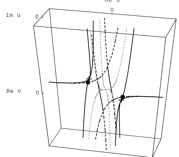
Figure 1: The $Im\,v=0$ hypersurface of the $G_{2}$ moduli space. The light dotted curve is given by the vanishing of the classical discriminant $\Delta_{cl}=0$. Classically the $v=0$ plane is also a singular surface. The heavy solid and dashed curves are the singular surfaces $\Delta_{\pm}=0$ where dyons become massless. Points marked with a ‘$\bullet$’ indicate transversal intersections where two mutually local dyons become massless, while at points marked with a ‘${\bf+}$’ mutually non-local dyons become massless. (Other such points occur at $Im\,v\neq 0$.)

Let us now compare this information with that contained in the Riemann surfaces of [7] and [3, 4]. We start with the curve from the integrable system. It is given by the expression

$${\cal C}_{int}=3(z-\frac{\mu}{z})^{2}-x^{8}+2ux^{6}-\left[u^{2}+6(z+\frac{\mu}{z})\right]x^{4}+\left[v+2u(z+\frac{\mu}{z})\right]x^{2}=0\,.$$ (13)

As explained in [7] one can view this as an eight-sheeted cover of the $z$-plane. The parameter $\mu$ is related to the scale $\Lambda_{H}$. We are interested in its singularities and therefore look at

$$\frac{\partial{\cal C}}{\partial z}={2\over z^{3}}(-\mu+z^{2})(3\mu+ux^{2}z-3x^{4}z+3z^{2})=0\,.$$ (14)

This gives rise to two inequivalent branches of solutions for $z$. The first one is given by $z=\pm\sqrt{\mu}$. Substituting this back into (13) gives polynomials of sixth order in $x$ of the form

$$P^{6}_{\pm}=x^{6}-2ux^{4}+u^{2}x^{2}\mp 12\sqrt{\mu}x^{2}-v\pm 4\sqrt{\mu}u\,.$$ (15)

The discriminants of these are given by

$$\Delta^{P}_{\pm} = (\mp 4\sqrt{\mu}\,u+v)\Delta^{int}_{\pm}\,,$$

$$\Delta^{int}_{\pm} = \mp 6912\sqrt{\mu^{3}}-144\mu u^{2}\mp 32\sqrt{\mu}\,u^{4}\pm 216\sqrt{\mu}uv-4u^{3}v+27v^{2}\,.$$ (16)

Both solutions of the second branch generate the same polynomial of eighth order

$$P^{8}=12x^{8}-12ux^{6}+4u^{2}x^{4}-3vx^{2}+36\mu\,,$$ (17)

whose discriminant is given by the product of $\Delta^{int}_{+}$ with $\Delta^{int}_{-}$. At this point it is important to recall that the construction of the curves in [7] was based on the dual (affine) Lie algebra. In order to compare (S0.Ex3) with (10) we should therefore perform a duality transformation as in (4). One finds then that after setting $\sqrt{\mu}=\frac{1}{6}\Lambda_{H}^{4}$ the factors $\Delta^{int}_{\pm}$ coincide precisely with (10)! It is natural then to conjecture that the prefactors in (S0.Ex3) are ‘accidental’ singularities where ramification points of (13) coincide without physical states becoming massless.

Furthermore, we can now classify which superconformal field theory sits at the points (12). For example, consider $P_{-}^{6}$ near the image of the point $(u_{0},v_{0})=(\sqrt{6}\Lambda_{H}^{2},-{2\sqrt{2}\over 3\sqrt{3}}\Lambda_{H}^{6})$ where it degenerates. One can easily show that it takes the form

$$P^{6}_{-}=y^{3}-y\delta u-\delta v\,,$$ (18)

where $y=x^{2}-2u/3$, $\delta u=\sqrt{8/3}\Lambda_{H}^{2}(u-u_{0})$, and $\delta v=v-v_{0}+2\Lambda_{H}^{4}(u-u_{0})$ and $u_{0},v_{0}$ are now in the dual coordinates. Similar considerations apply to $P^{8}$. Thus the singularity at this point is of type $A_{2}$ and we find a superconformal field theory of the same type as in [14].

Let us turn now to the hyperelliptic curve [3, 4]. It can be written as

$$y^{2}=\left[x^{2}(x^{2}-u)^{2}-v\right]^{2}-\Lambda^{8}x^{4}\,,$$ (19)

and its discriminant is given by

$$v\Delta^{h}_{+}\Delta^{h}_{-} = v(4\Lambda^{12}+8\Lambda^{8}u^{2}+4\Lambda^{4}u^{4}-36\Lambda^{4}uv-4u^{3}v+27v^{2})$$ (20)

$$(-4\Lambda^{12}+8\Lambda^{8}u^{2}-4\Lambda^{4}u^{4}+36\Lambda^{4}uv-4u^{3}v+27v^{2})\,.$$

The first observation is that no redefinition of the gauge invariant variables can bring this into the form (10). That really the topology of (20) is different from what we had before can also be seen from the fact that $\Delta^{h}_{+}$ and $\Delta^{h}_{-}$ intersect each other transversally in eight points which group themselves into two sets of four ($n=0,\ldots,3$)

$$(u,v)_{\pm} = (e^{\frac{i\pi n}{2}}\sqrt[4]{37\pm 14\sqrt{7}}\Lambda^{2},-e^{\frac{i3\pi n}{2}}\frac{2}{27}(17\mp 7\sqrt{7})\sqrt[4]{(37\pm 14\sqrt{7})^{3}}\Lambda^{6})\,.$$ (21)

Further the discriminant (20) has an overall factor of $v$. Thanks to the curve being hyperelliptic it is not very complicated to study explicitly the monodromy around this singularity. In order to do so we go to a scaling limit where $x=\epsilon z/u$, $v=\epsilon^{2}\rho$ and $\epsilon\rightarrow 0$. Then the curve becomes

$$y^{2}\cong\epsilon^{4}[(z^{2}-\rho)^{2}-({\Lambda^{2}\over u})^{4}z^{4}].$$ (22)

There are four branch points of this curve, $\pm e_{1}$ and $\pm e_{2}$ where

$$e_{1}=\sqrt{\rho\over{1+({\Lambda^{2}\over u})^{2}}},e_{2}=\sqrt{\rho\over{1-({\Lambda^{2}\over u})^{2}}}.$$

Under $v\rightarrow ve^{2\pi i}$ all the branch points rotate in the x-plane by $e^{\pi i}$. Therefore a loop around $v=0$ induces a monodromy which simply flips the signs of a pair of dual homology cycles $(\alpha_{i},\beta_{i})$. We could then choose a basis such that $(e^{D}_{i},e_{i})=\oint_{(\beta_{i},\alpha_{i})}\lambda$ and find that say $(e^{D}_{1},e_{1})\rightarrow(-e^{D}_{1},-e_{1})$ while the others stay fixed. Already this seems to be a problem because the Weyl group of $G_{2}$ does not contain such an element and moreover it violates the constraint $\sum_{i}e_{i}=0$.

Let us nonetheless continue to study the physical implications of this singularity by studying the effective $U(1)$ gauge theory associated with the $(\alpha,\beta)$ cycles. To simplify the analysis we fix $u$ and $\Lambda$ such that $\delta={\Lambda^{4}\over{2u^{2}}}$ is a small parameter and use the one form $\lambda=(-4x^{6}+4ux^{4}-2v){dx\over y}$ to solve for the gauge coupling. We find

$$a=\int_{\alpha}\lambda\cong 2\pi i{\sqrt{v}\over{u}}+{\cal O}(\delta^{2})$$

$$a_{D}=\int_{\beta}\lambda\cong 4{\sqrt{v}\over{u}}\ln{\delta\over{4}}+{\cal O}(\delta)$$

$$\tau={\partial a_{D}\over{\partial a}}\cong{2\over{\pi i}}\ln{\delta\over{4}}+{\cal O}(\delta)$$

Note that $\tau$ is scale invariant for fixed $\delta$ since it does not depend on $\epsilon$,$\rho$, or $v$.

Now we define $q=e^{\pi i\tau}$ and substitute into (22) which gives

$$y^{2}_{eff}=(z^{2}-\rho)^{2}-64qz^{4}.$$

Finally, we compare this to the $SU(2)$ curve with $N_{f}=4$ massless flavors [1, 18] and find that they are equivalent in the limit of small $q$. Indeed the $SU(2)$ monodromy is just $(a_{D},a)\rightarrow(-a_{D},-a)$. Therefore we conclude that the physics at the $v=0$ singularity is a non-abelian Coulomb phase with an enhanced $SU(2)$ gauge symmetry. This leads us to an alternative physical interpretation of the curve (19). If we start with the $SU(6)$ curve with $N_{f}=4$ massless flavors [17]

$$y^{2}=(x^{6}+\sum_{i=2}^{6}s_{i}x^{6-i})^{2}-\Lambda^{8}x^{4}$$ (23)

and make a restriction of the moduli space to ($s_{1}=s_{3}=s_{5}=0$, $s_{2}=-2u$, $s_{4}=u^{2}$, $s_{6}=-v$), we get the same curve as the $G_{2}$ ansatz. Now the physics at $v=0$ has a clear interpretation as a point on the mixed Higgs-Coulomb branch where classically there is an unbroken $SU(2)$ gauge symmetry with $4$ massless flavors which is expected to remain quantum mechanically [19].

This analysis together with the fact that the $G_{2}$ ansatz predicts more than four $N\!=\!1$ vacua (as well as other strong coupling monodromies which don’t have a clear interpretation) raises serious doubts about the role of the hyperelliptic curve in describing the strong coupling physics of $G_{2}$. In contrast, although not obviously arising from a hyperelliptic curve, the discriminant (10) seems to have the correct properties to describe $G_{2}$ and in particular exhibits the expected splitting of the classical vacua into pairs of singularities.

Certainly our analysis was based on the assumption that the superpotential (8) is exact. As emphasized in [10], a priori one cannot exclude a correction term $W_{\Delta}$. In practically all the examples however it proved to be correct to assume $W_{\Delta}=0$, the only exception being the case of $SO(2r+1)$ where the particular form of $W_{\Delta}$ just amounted to a redefinition of the gauge invariant variables similar to the duality transformation we encountered here. We therefore feel confident that the superpotential (8) represents the physics correctly.

We now treat the case of the $G_{2}$ theory with matter hypermultiplets in the fundamental representation. Before doing so however, it is instructive to consider the case of $SO(5)$ with one hypermultiplet. The reason for this is that both models share the essential physics and we can compare our results for $SO(5)$ with the known curve of [20]. The gauge invariant variables are $u=e_{1}^{2}+e_{2}^{2}$ and $v=-e_{1}^{2}e_{2}^{2}$. The tree-level superpotential is

$$W_{tree}={\tilde{Q}}\Phi{Q}+m{\tilde{Q}}{Q}+g_{1}u+g_{2}v\,.$$ (24)

As before, we want to consider classical vacua that break $SO(5)\rightarrow SU(2)\times U(1)$ which leads to

$$\Phi_{cl}=\left(\matrix{0&ie&0&0&0\cr-ie&0&0&0&0\cr 0&0&0&ie&0\cr 0&0&-ie&0&0\cr 0&0&0&0&0}\right)\ .$$ (25)

Straightforward computation shows $e^{2}={g_{1}\over{g_{2}}}$. Since the fundamental of $SO(5)$ decomposes as ${\bf 2}+\bar{\bf 2}+{\bf 1}$, at low energies we find an $SU(2)$ theory with two matter hypermultiplets of masses $m_{+}=m+e$ and $m_{-}=m-e$. The effective superpotential at low energies is therefore

$$W_{L}=m_{+}V^{12}+m_{-}V^{34}+X(Pf(V)-\Lambda_{L}^{4})+g_{1}u+g_{2}v.\,,$$ (26)

Here $V^{ij}=Q^{i}Q^{j}$ is the antisymmetric tensor containing the gauge invariant bilinears of the $SU(2)$ theory and $X$ is a Lagrange multiplier [21]. We also need the scale-matching condition which in this case reads $\Lambda^{4}_{L}=4g_{1}g_{2}\,\Lambda^{4}_{SO(5)}$. Eliminating $V^{ij}$ and $X$ by their equations of motion results in

$$W_{L}=\frac{g_{1}^{2}}{g_{2}}\pm 2\sqrt{m^{2}-\frac{g_{1}}{g_{2}}}\sqrt{g_{1}g_{2}}\Lambda_{SO(5)}^{2}\,.$$ (27)

The vev’s of the gauge invariant variables are then given by

$$\langle u\rangle = 2e^{2}\mp\frac{e\,\Lambda_{SO(5)}^{2}}{\sqrt{m^{2}-e^{2}}}\pm\sqrt{m^{2}-e^{2}}\,\frac{\Lambda_{SO(5)}^{2}}{e}\,,$$ (28)

$$\langle v\rangle = -e^{4}\pm\frac{e^{3}\Lambda_{SO(5)}^{2}}{\sqrt{m^{2}-e^{2}}}\pm\sqrt{m^{2}-e^{2}}\,e\,\Lambda_{SO(5)}^{2}$$ (29)

Upon eliminating $e$ we find that the discriminant is

$$\Delta^{N_{f}=1}_{SO(5)} = -16\,{\Lambda_{SO(5)}^{12}}\,{m^{4}}-27\,{\Lambda_{SO(5)}^{8}}\,{m^{8}}+36\,{\Lambda_{SO(5)}^{8}}\,{m^{6}}\,u-8\,{\Lambda_{SO(5)}^{8}}\,{m^{4}}\,{u^{2}}+$$

$${\Lambda_{SO(5)}^{4}}\,{m^{6}}\,{u^{3}}-{\Lambda_{SO(5)}^{4}}\,{m^{4}}\,{u^{4}}+24\,{\Lambda_{SO(5)}^{8}}\,{m^{4}}\,v+16\,{\Lambda_{SO(5)}^{8}}\,{m^{2}}\,u\,v+$$

$$36\,{\Lambda_{SO(5)}^{4}}\,{m^{6}}\,u\,v-46\,{\Lambda_{SO(5)}^{4}}\,{m^{4}}\,{u^{2}}\,v+8\,{\Lambda_{SO(5)}^{4}}\,{m^{2}}\,{u^{3}}\,v-{m^{4}}\,{u^{4}}\,v+$$

$${m^{2}}\,{u^{5}}\,v+16\,{\Lambda_{SO(5)}^{8}}\,{v^{2}}+24\,{\Lambda_{SO(5)}^{4}}\,{m^{4}}\,{v^{2}}-64\,{\Lambda_{SO(5)}^{4}}\,{m^{2}}\,u\,{v^{2}}+$$

$$8\,{\Lambda_{SO(5)}^{4}}\,{u^{2}}\,{v^{2}}-8\,{m^{4}}\,{u^{2}}\,{v^{2}}+8\,{m^{2}}\,{u^{3}}\,{v^{2}}+{u^{4}}\,{v^{2}}-32\,{\Lambda_{SO(5)}^{4}}\,{v^{3}}-$$

$$16\,{m^{4}}\,{v^{3}}+16\,{m^{2}}\,u\,{v^{3}}+8\,{u^{2}}\,{v^{3}}+16\,{v^{4}}\,.$$

As in the case without matter [11] this matches the discriminant of the curve [20]

$$y^{2}=(x^{4}-x^{2}u-v)^{2}-\Lambda_{SO(5)}^{4}x^{2}(x^{2}-m^{2})\,,$$ (31)

after rescaling $\Lambda_{SO(5)}$ and up to an overall factor of $v$. We take this as convincing evidence for the method.

It is relatively straightforward to generalize to the case with $N_{f}$ flavors using the results of [21]. We find a low energy superpotential

$$W_{L}={g_{1}^{2}\over g_{2}}\pm 2\sqrt{g_{1}g_{2}}\sqrt{Pf(\tilde{m})}\,\Lambda_{SO(5)}^{3-N_{f}},$$ (32)

where $Pf(\tilde{m})=\prod_{i=1}^{N_{f}}(m_{i}^{2}-{g_{1}\over g_{2}})$, from which we can determine $\langle u\rangle$, $\langle v\rangle$, and discriminant in the usual way. For $N_{f}=2$ we find agreement with the curve in [20].

Having discussed the case of $SO(5)$ in detail it is straightforward to treat $G_{2}$ now. The fundamental of $G_{2}$ decomposes under $SU(2)$ according to ${\bf 7}\rightarrow{\bf 2}+\bar{\bf 2}+3\cdot{\bf 1}$. At low energies we thus have the same theory as before. The scale matching condition is replaced by $\Lambda_{L}^{4}=-g_{1}g_{2}\Lambda_{H}^{6}$ and $\Phi_{cl}$ is the same as without matter. For the gauge invariant variables we obtain

$$\langle u\rangle = 3e^{2}\pm\frac{\Lambda_{H}^{3}}{4\sqrt{m^{2}-e^{2}}}\mp\sqrt{m^{2}-e^{2}}\frac{\Lambda_{H}^{3}}{2e^{2}}\,,$$ (33)

$$\langle v\rangle = 4e^{6}\pm\frac{e^{4}\Lambda_{H}^{3}}{\sqrt{m^{2}-e^{2}}}\pm 2\sqrt{m^{2}-e^{2}}\,e^{2}\Lambda_{H}^{3}\,,$$ (34)

from which we can in principle compute the discriminant by eliminating $e$. For the case with $m=0$ we find

$$\Delta^{N_{f}=1}_{G2} = 8v(4u^{3}-27v)^{2}+8748\Lambda_{H}^{6}v^{2}+2160\Lambda_{H}^{6}u^{3}v+4374\Lambda_{H}^{12}v$$ (35)

$$+54\Lambda_{H}^{12}u^{3}+729\Lambda_{H}^{18}\,.$$

It would be extremely interesting to see which kind of Riemann surface reproduces this result. Again the generalization to $N_{f}$ flavors is given by a low energy superpotential

$$W_{L}=i\sqrt{\frac{g_{1}^{3}}{g_{2}}}\pm 2i\sqrt{g_{1}g_{2}}\sqrt{Pf(\tilde{m})}\,\Lambda_{G_{2}}^{4-N_{f}}$$ (36)

with $Pf(\tilde{m})=\prod_{i=1}^{N_{f}}(m_{i}^{2}-e^{2})$ which leads to

$$\langle u\rangle = 3e^{2}\pm\frac{\Lambda_{H}^{4-N_{f}}}{4\,\sqrt{Pf({\tilde{m}})}}\sum_{i=1}^{N_{f}}\prod_{j\neq i}(m_{j}^{2}-e^{2})\mp\sqrt{Pf({\tilde{m}})}\frac{\Lambda_{H}^{4-N_{f}}}{2e^{2}}\,,$$ (37)

$$\langle v\rangle = 4e^{6}\pm\frac{e^{4}\Lambda_{H}^{4-N_{f}}}{\sqrt{Pf({\tilde{m}})}}\sum_{i=1}^{N_{f}}\prod_{j\neq i}(m_{j}^{2}-e^{2})\pm 2\sqrt{Pf({\tilde{m}})}\,e^{2}\Lambda_{H}^{4-N_{f}}\,.$$ (38)

We can recover results for fewer flavors by taking some quark mass $m_{i}\rightarrow\infty$ while keeping $m_{i}(\Lambda_{N_{f}})^{4-N_{f}}=(\Lambda_{N_{f}-1})^{5-N_{f}}$ held fixed.

Acknowledgements

The research of K.L. is supported in part by the Fonds zur Förderung der wissenschaftlichen Forschung under Grant J01157-PHY and by DOE grant DOE-91ER40618. That of J.M.P. and S.B.G. is partially supported by DOE grant DOE-91ER40618 and by NSF PYI grant PHY-9157463.

References

• [1] N. Seiberg and E. Witten, Nucl. Phys. B426 (1994) 19, hep-th/9407087;
N. Seiberg and E. Witten, Nucl. Phys. B431 (1994) 484, hep-th/9408099.
• [2] A. Klemm, W. Lerche, S. Theisen, and S. Yankielowicz, Phys. Lett. B344 (1995) 169, hep-th/9411048;
P. Argyres and A. Faraggi, Phys. Rev. Lett. 73 (1995) 3931, hep-th/9411057;
A. Hanany and Y. Oz, Nucl. Phys. B452 (1995) 283, hep-th/9505075;
P. Argyres, M. Plesser, and A. Shapere, Phys. Rev. Lett. 75 (1995) 1699, hep-th/9505100;
U. Danielsson and B. Sundborg, Phys. Lett. B358 (1995) 273, hep-th/9504102;
J. A. Minahan and D. Nemeschansky Nucl. Phys. B464 (1996) 3, hep-th/9506198;
A. Brandhuber and K. Landsteiner Phys. Lett. 358 (1995) 73, hep-th/9507008;
A. Hanany, Nucl. Phys. B466 (1996) 85, hep-th/9509176;
P. C. Argyres and A. D. Shapere Nucl. Phys. B461 (1996) 437, hep-th/9509175.
• [3] U. Danielsson and B. Sundborg, Phys. Lett. B370 (1996) 370, hep-th/9511180.
• [4] M. Alishahiha, F. Ardalan, and F. Mansouri, The Moduli Space of the Supersymmetric G(2) Yang-Mills Theory, preprint IPM-95-117, hep-th/9512005.
• [5] M. R. Abolhasani, M. Alishahiha, and A. M. Ghezelbash, The Moduli Space and Monodromies of the $N\!=\!2$ Supersymmetric Yang-Mills Theory with any Lie Gauge Groups, preprint IPM-96-144, hep-th/9606043.
• [6] A. Gorsky, I. Kriechever, A. Marshakov, A. Mironov, and A. Morozov, Phys. Lett. B355 (1995) 466, hep-th/9505035.
• [7] E. Martinec and N. P. Warner, Nucl. Phys. B459 (1996) 97, hep-th/9509161.
• [8] R. Donagi and E. Witten, Nucl. Phys. B460 (1996) 299, hep-th/9510101.
• [9] A. Klemm, W. Lerche, P. Mayr, C. Vafa and N. Warner, Self-Dual Strings and $N\!=\!2$ Supersymmetric Field Theory, preprint CERN-TH-96-95, HUTP-96/A014, USC-96/008, hep-th/9604034;
K. Landsteiner, E. Lopez and D. Lowe, Evidence for S-Duality in $N\!=\!4$ Supersymmetric Yang-Mills Theory, preprint UCSBTH-96-14, NSF-ITP-96-58, hep-th/9606146;
C. Gomez, R. Hernandez and E. Lopez, K3 Fibrations and Softly broken $N\!=\!4$ Supersymmetric Gauge Theories, preprint NSF-ITP-96-75, hep-th/9608104;
S. Nam Integrable Structure in SUSY Gauge Theories and String Duality, hep-th/9607223;
W. Lerche and N. P. Warner, Exceptional SW Geometry from ALE Fibrations, hep-th/9608183.
• [10] S. Elitzur, A. Forge, A. Giveon, K. Intriligator, and E. Rabinovici, Phys. Lett. B379 (1996) 121, hep-th/9603051.
• [11] S. Terashima and S.-K. Yang, Confining Phase of $N\!=\!1$ Supersymmetric Gauge Theories and $N\!=\!2$ Massless Solitons, preprint UTHEP-340, hep-th/9607151.
• [12] I. Pesando, Mod. Phys. Lett. A10 (1995) 1871,hep-th/9506139;
S.B. Giddings and J. Pierre, Phys. Rev. D52 (1995) 6065, hep-th/9506196;
P. Pouliot, Phys. Lett. B356 (1995) 108.hep-th/9507018.
• [13] D. Kutasov, A. Schwimmer, and N. Seiberg, Nucl. Phys. B459 (1996) 455, hep-th/9510222.
• [14] P. Argyres and M. Douglas, Nucl. Phys. B448 (1995) 93, hep-th/9505062.
• [15] P. C. Argyres, M. R. Plesser, N. Seiberg, and E. Witten, Nucl. Phys. B461 (1996) 71, hep-th/9511154;
T. Eguchi, K. Hori, K. Ito, and S.-K. Yang, Nucl. Phys. B471 (1996) 430, hep-th/9603002.
• [16] R. Donagi, Decomposition of spectral covers in Journées de Geometrie Algébrique d’Orsay, Asterisque vol. 218, Soc. Math. de France, Paris (1993).
• [17] A. Hanany and Y. Oz, as in [2].
• [18] P. C. Argyres and A. D. Shapere, as in [2].
• [19] P. C. Argyres, M. R. Plesser, and N. Seiberg, Nucl. Phys. B471 (1996) 159, hep-th/9603042.
• [20] A. Hanany, as in [2].
• [21] N. Seiberg, Phys. Rev. D49 (1994) 6857, hep-th/9402044.