Masses of the physical mesonsfrom an effective QCD–Hamiltonian

Abstract

The front form Hamiltonian for quantum chromodynamics, reduced to an effective Hamiltonian acting only in the $q\bar{q}$ space, is solved approximately. After coordinate transformation to usual momentum space and Fourier transformation to configuration space a second order differential equation is derived. This retarded Schrödinger equation is solved by variational methods and semi-analytical expressions for the masses of all 30 pseudoscalar and vector mesons are derived. In view of the direct relation to quantum chromdynamics without free parameter, the agreement with experiment is remarkable, but the approximation scheme is not adequate for the mesons with one up or down quark. The crucial point is the use of a running coupling constant $\alpha_{s}(Q^{2})$, in a manner similar but not equal to the one of Richardson in the equal usual-time quantization. Its value is fixed at the Z mass and the 5 flavor quark masses are determined by a fit to the vector meson quarkonia.

Preprint MPIH-V34-1996

Submitted to Physical Review D (1996)
PACS-Index: 12.40.Yx, 11.10.Ef, 11.15.Tk

Revision of MPIH-V45-1995 (2 December 1995)
Internet: pauli@zooey.mpi-hd.mpg.de

1 Introduction and motivation

One of the most outstanding tasks in strong interaction physics is to calculate the spectrum and the wavefunctions of physical hadrons from quantum chromodynamics (QCD). Discretized light-cone quantization (DLCQ) [1] has precisely this goal. Its three major aspects are: (1) a rejuvenation of the Hamiltonian approach, (2) a denumerable Hilbert space of plane waves, and (3) Dirac’s front form of Hamiltonian Dynamics. In the front form [2], or in light-cone quantization [3], one quantizes at equal ‘light-cone time’ $x^{+}=t+z$, as opposed to the conventional instant form where one quantizes at equal usual time $t$. As reviewed in [4], the front form has unique features, among them: The vacuum is simple, or at least simplier than in the instant form, and the relativistic wavefunctions transform trivially under certain boosts [2, 4]. Both are in stark contrast to the conventional instant form. Over the years, the light-cone approach [5] has made much progress. Calculations [4] agree with other methods particularly lattice gauge theory. Zero modes of the fields can be important carriers of quantum structures [6], particularly of those of the vacuum [7, 8]. Dimensionally reduced models [7, 8] provide much insight into the structure of possible solutions to QCD. But chiral aspects are not yet understood, and non-perturbative renormalization remains a challenge [9, 10] as for any Hamiltonian approach.

But despite the many successes of light-cone Hamiltonian methods one misses the contact to phenomenology beyond the perturbative regime. We believe that more QCD-inspired approaches are needed, work like for example [11, 12] or [13, 14], where the formalism is related to the experiment. The present work is of this type.

Right from the outset when applying DLCQ to gauge theory in 3+1 dimensions [15, 16, 17] it was clear that one should need an effective Hamiltonian. In [16] an integral equation in the light-cone momenta was solved numerically, which was derived by procedures similar to those of Tamm and Dancoff [18, 19], and a non-integrable singularity was removed by an ad hoc assumption. But recently [20] the method of effective interactions was generalized to avoid the usual truncation in the particle number [21]. As it turns out, one can assemble all many-body aspects into a vertex function which bears great similarity with the running coupling constant.

One wonders: How can such a simple structure account for the spectra and wavefunctions of all scalar and vector mesons? Is this not too much of a claim? On the other hand the effective Hamiltonian has been derived [21] from the QCD-Lagrangian without condition on the coupling constant or on the mass of the constituents. One way of checking this is to compare to experiment, and this shall be done in this work very roughly and preliminarily. Lacking the running coupling constant going with the theory [21], one can replace it by one of its current phenomenological versions [22, 23, 24]. The present work applies the one of Richardson [22]. It interpolates smoothly between asymptotic freedom [25, 26] and infrared slavery. After that, one has no freedom in the theory and no adjustable parameters. Since the quark masses cannot be determined from independent measurements, they must be determined self-consistently from a fit to some of the meson masses. This in itself is not trivial, except when having analytical expressions.

In particular, a coordinate transformation from front to instant-form coordinates is performed in Section 3. Apart from a more transparent interpretation, this way of writing down the integral equation has certain advantages in performing the calculations. No assumptions will be made in this section: All manipulations are straightforward and fully equivalent to the front-form formulation. In Section 4, the bound-state equation is approximated semi-relativistically which allows for Fourier transforming the momentum-space integral equation into a configuration-space Schrödinger type equation. The so obtained Hamiltonian is reduced in Section 5 to a minimal number of terms (Coulomb plus linear potential plus one spin-dependent term distinguishing between singlet and triplet) and diagonalized approximately by a variational method.

The masses of all pseudoscalar and vector mesons in Section 6 are thus semi-analytic and approximate solutions to a second order differential equation in configuration space. In comparison with the empirical masses [28], they are not much worse than those of potential models [29, 30, 31, 32, 33], or predictions from heavy quark symmetry [34], or even predictions based on lattice gauge calculations [35, 36, 37]. In view of the direct link to QCD [21] and the simplicity this should be regarded as considerable progress in the front-form approach.

But there is a potential danger in such an endeavor. The present work is motivated by the question whether the simple structures to be displayed can describe experiments at all. Obviously they can, but it should be emphasized that numerically accurate solutions need another effort. This is currently being attempted [38] and has a different objective than to develop models designed to reproduce the data.

2 The effective Hamiltonian for QCD

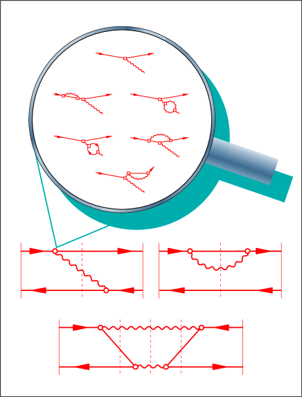
Figure 1: The effective interaction in the $q\bar{q}$ sector. By exchanging ‘effective gluons’, a single quark state with four-momentum $k_{1}$ and spin projection $\lambda_{1}$ is scattered into the quark state ($k_{1}^{\prime},\lambda_{1}^{\prime}$). Correspondingly, the antiquark is scattered from ($k_{2},\lambda_{2}$) to ($k_{2}^{\prime},\lambda_{2}^{\prime}$).

Figure 2: The quark-antiquark potential $V(r)$ as given in Eq.(11) is plotted versus the relative distance $r$. The Coulomb and the confining potential are indicated. Some of the heavier meson masses are inserted to provide a scale.

In Discretized Light-Cone Quantization (DLCQ) one seeks to solve the eigenvalue problem

$$H_{\rm LC}|\Psi_{b}\rangle=M_{b}^{2}|\Psi_{b}\rangle$$ (1)

for a field theory. The ‘light-cone Hamiltonian’ $H_{\rm LC}\equiv P^{\mu}P_{\mu}$ [4] is the Lorentz invariant contraction of the energy-momentum four-vector $P^{\mu}$ and has the dimension $<\!\!mass\!\!>^{2}$. The eigenvalues $M_{b}^{2}$ are interpreted as the square of the invariant mass of state $b$. Working in momentum representation, the three space-like components of $P^{\mu}$ are diagonal operators, with eigenvalues $P^{+}=\sum_{j}k^{+}_{j}$ and $\vec{P}_{\!\bot}=\sum_{j}\vec{k}_{\!\bot_{j}}$. The sum runs over all particles in a Fock state. Each particle has a four-momentum denoted by $k^{\mu}_{j}=(k^{+}_{j},\vec{k}_{\!\bot_{j}},k^{-}_{j})$ and sits on its mass shell $(k^{\mu}k_{\mu})_{j}=m_{j}^{2}$. The time-like component, the Hamiltonian proper $P^{-}$, is a complicated and off-diagonal operator acting in Fock space. Its matrix elements are tabulated in [4]. Based on the boost-properties of light-cone operators [4] one can transform to a frame where $\vec{P}_{\!\bot}=0$, thus $P^{\mu}P_{\mu}=P^{+}P^{-}$. Since $P^{+}$ is diagonal, the diagonalization of $P^{-}$ and of $H_{\rm LC}$ amounts to the same. The Hilbert space for diagonalizing $P^{-}$ is spanned by all Fock states which have given eigenvalues of $P^{+}$ and $\vec{P}_{\!\bot}=(0,0)$ and can be arranged into sectors according to the particle number like $q\bar{q}$, $q\bar{q}\,g$, or $q\bar{q}\,q\bar{q}$. For any fixed value of the harmonic resolution $K=2LP^{+}/\pi$, the Hamiltonian matrix in Eq.(1) is finite and in principle could be diagonalized numerically [1]. Details can be found in the literature [4, 20, 21].

DLCQ is quite useful to cleanly phrase the problem, but to do calculations particularly in 3+1 dimensions one has to develop effective Hamiltonians. Fock space truncation in conjunction with perturbation theory in the manner of Tamm and Dancoff [18, 19] is unsatisfactory, because one has to resort to ad hoc prescriptions to make things work [16]. These drawbacks can be avoided by the method of iterated resolvents [20, 21]. It turns out possible to convert the many-body matrix Eq.(1) into a well defined two-body equation with an effective interaction acting only in the $q\bar{q}$-space, i.e. $H_{\rm eff}|\psi_{b}\rangle=M_{b}^{2}|\psi_{b}\rangle$. In the continuum limit one has to solve the integral equation

$$M_{b}^{2}\langle x,\vec{k}_{\!\perp};\lambda_{1},\lambda_{2}|\psi_{b}\rangle=\sum_{\lambda_{1}^{\prime},\lambda_{2}^{\prime}}\!\int\!\!dx^{\prime}d^{2}\vec{k}_{\!\perp}^{\prime}\,\langle x,\vec{k}_{\!\perp};\lambda_{1},\lambda_{2}|H_{\rm eff}|x^{\prime},\vec{k}_{\!\perp}^{\prime};\lambda_{1}^{\prime},\lambda_{2}^{\prime}\rangle\,\langle x^{\prime},\vec{k}_{\!\perp}^{\prime};\lambda_{1}^{\prime},\lambda_{2}^{\prime}|\psi_{b}\rangle.$$ (2)

The bras and kets refer to $q\bar{q}$ Fock states which can be made invariant under $SU(N)$,

$$|x,\vec{k}_{\!\perp};\lambda_{1},\lambda_{2}\rangle={1\over\sqrt{n_{c}}}\sum_{c=1}^{n_{c}}b^{\dagger}_{c}(k_{1},\lambda_{1})d^{\dagger}_{c}(k_{2},\lambda_{2})|0\rangle.$$ (3)

Goal of the calculation are the momentum-space wavefunctions $\langle x,\vec{k}_{\!\perp};\lambda_{1},\lambda_{2}|\psi_{b}\rangle$. They are the probability amplitudes for finding the quark with helicity projection $\lambda_{1}$, longitudinal momentum fraction $x\equiv k_{1}^{+}/P^{+}$ and transversal momentum $\vec{k}_{\!\bot}$, and correspondingly the antiquark with $\lambda_{2}$, $1-x$ and $-\vec{k}_{\!\bot}$. The effective interaction as diagrammatically displayed in Figure 2 is a sum of three terms: The first two diagrams are kind of a one-gluon exchange and describe the flavor conserving part of the effective interaction, while the last graph due to the two-gluon annihilation can change the flavor. In the present work we deal only with the first of them. The kernel of the integral equation (2) has a diagonal ‘kinetic’ and an off-diagonal ‘interaction’ energy, i.e.

$$M_{b}^{2}\,\langle x,\vec{k}_{\!\perp};\lambda_{1},\lambda_{2}|\psi_{b}\rangle=\left[{m_{1}+\vec{k}_{\!\perp}^{2}\over x}+{m_{2}+\vec{k}_{\!\perp}^{2}\over 1-x}\right]\langle x,\vec{k}_{\!\perp};\lambda_{1},\lambda_{2}|\psi_{b}\rangle$$

$$-{1\over 4\pi^{2}}\sum_{\lambda_{1}^{\prime},\lambda_{2}^{\prime}}\!\int\!\!dx^{\prime}d^{2}\vec{k}_{\!\perp}^{\prime}\,\Theta(x^{\prime},\vec{k}_{\!\perp}^{\prime})\,{\beta(Q)\over Q^{2}}\,{\langle\lambda_{1},\lambda_{2}|S(Q)|\lambda_{1}^{\prime},\lambda_{2}^{\prime}\rangle\over\sqrt{x(1-x)x^{\prime}(1-x^{\prime})}}\,\langle x^{\prime},\vec{k}_{\!\perp}^{\prime};\lambda_{1}^{\prime},\lambda_{2}^{\prime}|\psi_{b}\rangle.$$ (4)

The most important factors are the four-momentum transfer

$$Q^{2}=-(k_{1}-k_{1}^{\prime})^{2}=-(k_{2}-k_{2}^{\prime})^{2}$$ (5)

and the vertex function $r(Q,\Lambda)$ which likes to combine with the coupling constant $g$ to become

$$\beta(Q)={n_{c}^{2}-1\over 2n_{c}}\ {g^{2}\over 4\pi\hbar c}\ r^{2}(Q,\Lambda)\equiv{4\over 3}\alpha_{s}(Q),$$ (6)

the like-to-be ‘running coupling constant’. For QED, this factor reduces to the fine structure constant $\beta=\alpha\sim 1/137$. The spinor factor $S(Q)$ represents the familiar current-current coupling

$$\langle\lambda_{1},\lambda_{2}|S(Q)|\lambda_{1}^{\prime},\lambda_{2}^{\prime}\rangle=\left[\overline{u}(k_{1},\lambda_{1})\,\gamma^{\mu}\,u(k_{1}^{\prime},\lambda_{1}^{\prime})\right]\left[\overline{u}(k_{2},\lambda_{2})\,\gamma_{\mu}\,u(k_{2}^{\prime},\lambda_{2}^{\prime})\right].$$ (7)

The cut-off function $\Theta(x^{\prime},\vec{k}_{\!\perp}^{\prime})$ restricts integration in line with Lepage-Brodsky regularization [4]

$$\Theta(x,\vec{k}_{\!\perp}):\qquad\qquad{m_{1}^{2}+\vec{k}_{\!\bot}^{\,2}\over x}+{m_{2}^{2}+\vec{k}_{\!\bot}^{\,2}\over 1-x}\leq(m_{1}+m_{2})^{2}+\Lambda^{2}.$$ (8)

The mass scale $\Lambda$ can be chosen freely.

Despite having been derived in the light-cone gauge $A^{+}=0$, the effective interaction is manifestly gauge invariant, depending only on the quark currents. The instantaneous interaction has cancelled exactly against other gauge-variant terms, see [15, 16, 21]. Since one works in the front form, it is also frame and boost invariant. Explicit calculations for QED [16, 38] are numerically very stable, and reproduce quantitatively the Bohr spectra and the fine and hyperfine structure.

The vertex function hidden in the like-to-be running coupling constant of Eq.(5) has the same perturbative series expansion as the running coupling constant [21] which is indicated in an artists way in Figure 2. What is missing, thus far, is a renormalization group analysis of the formal expressions. In the absence of that, we are interested in consequences of Eq.(5). How can it be that such a simple expression accounts for hadronic phenomena? What are the invariant masses of the pseudoscalar and vector mesons, using such an interaction? How far does one get with analytical procedures, and in particular where does the approach go wrong?

Lacking an exact expression for $\alpha_{s}(Q^{2})$, one can resort to reasonable parametrizations [22, 23, 24]. In the sequel, we shall content ourselves with the form of Richardson [22],

$$\alpha_{s}(Q^{2})=\frac{12\pi}{27}\,\frac{1}{\ln(a^{2}+Q^{2}/\kappa^{2})}\ .$$ (9)

At least, this form interpolates smoothly between asymptotic freedom [25, 26] and infrared slavery. In the original work, the the parameter $a$ was set to have the value $a=1$ and $\kappa$ was kept as free parameter to be determined by the spectra. Here, we take the value of $\alpha_{s}(M_{Z})=0.1134\pm 0.0035$ as measured at the Z-mass [28] to fix

$$\kappa=193\,{\rm MeV}\ .$$ (10)

Its Fourier transform [22] generates two terms, see also below,

$$V(\vec{x}\,)={-1\over 2\pi^{2}}\int\!\!d^{3}\vec{q}\ {\rm e}^{i\vec{q}\cdot\vec{x}}\ {\alpha_{s}(\vec{q}^{\,2})\over\vec{q}^{\,2}}={8\pi\over 27}\Big{(}-\frac{1}{r}+\kappa^{2}\,r\Big{)}\ ,$$ (11)

a (strong) Coulomb and a linearly rising potential, as plotted in Figure 2 versus $r=|\vec{x}|$. The linearity of the confining potential is a consequence of $a=1$, as used in [22] and throughout the present work. If one varies $a$ one gets the curves displayed in Figure 4. It is taken from [27]. Here, we do not want to keep $a$ as a free parameter. For one reason, we refuse to speculate at this point whether the potential is strictly confining or not. For the other reason, the results to be displayed below are not very sensitive to large distances since the wavefunctions decay rapidly. Last but not least, one has to await the renomalization group analysis of the $\alpha_{s}(Q)$ which truly comes with the theory [21].

Figure 3: The confining potential as function of the parameter $a$. Values are from top to bottom: $a=1$, $a=1.0005$, $a=1.01$, and $a=\sqrt{e}\simeq 1.65$.

Figure 4: Bound states of $q\bar{q}$-pairs versus quark masses. All masses are given in units of the QCD-scale $\kappa$. The upper curve refers to the triplet ($S_{e}=2$), the lower to the singlet ($S_{e}=0$). The masses of some vector mesons ($\rho^{0},\omega,\phi,J/\psi$) are marked by a ($\triangle$), those of the some pseudoscalars ($\pi^{0},\eta,\eta^{\prime},\eta_{c}$) by a ($\star$).

The flavor quark masses are then the only free parameters of the approach. Of course, they are subject to be determined consistently by experiment. Natural candidates are the masses of the pseudoscalar ($0^{-}$) and vector mesons ($1^{-}$). Since the flavor quark masses potentially range from a few MeV up to some 100 GeV, see for instance Figure 4, one faces two problems: (1) By good reasons, the numerical solutions of the integral equation have been restricted thus far to systems with equal masses of the constituents like positronium [16, 38]. The wave function is then peaked at $x=m_{1}/(m_{1}+m_{2})=1/2$. For very asymmetric systems this will be a problem. To avoid that, we shall identically rewrite the integral equation in the next section in terms of instant-form variables, which are somewhat easier to deal with. (2) Shall one really perform a calculation of similar complexity as in preceeding work [16, 38] for any given set of $m_{1}$ and $m_{2}$ when intending to fit them to the meson masses, or shall one aim for a quasi-analytic but approximate solution? In view of the preliminary character of the present study, we have opted for the second. At least, this will pave the way for a future and improved solution.

In the sequel, we shall replace $H_{\rm eff}$ by the operator

$$H={1\over 2(m_{1}+m_{2})}\left(H_{\rm eff}-(m_{1}+m_{2})^{2}\right)\ .$$ (12)

It differs from $H_{\rm eff}$ by an additive constant and an overall scale, which both are Lorentz scalars. Both $H$ and its eigenvalue $E$ have the dimension of a $\langle mass\rangle$ and have much in common with the non-relativistic Hamiltonian and the binding energy $E$, as we shall see. As compared to an instant-form Hamiltonian, however, the main advantages of the front-form $H_{\rm eff}$ as given in Eq.(5) prevail, namely the additivity of the interaction and the Lorentz invariance of the eigenvalues. — The rest of this work is a simple and straightforward evaluation.

3 Transforming variables from the front to the instant form

The single-particle four-momenta can be parametrized either in the front form, $k^{\mu}_{1}=(k^{+}_{1},\vec{k}_{\!\bot},k^{-}_{1})$ and $k^{\mu}_{2}=(k^{+}_{2},-\vec{k}_{\!\bot},k^{-}_{2})$, or in the instant form,

$$k^{\mu}_{1}=(k^{0}_{1},\vec{k}_{\!\bot},k_{z})=(E_{1},\vec{k}),\quad{\rm and}\quad k^{\mu}_{2}=(k^{0}_{2},-\vec{k}_{\!\bot},-k_{z})=(E_{2},-\vec{k})\ .$$ (13)

Since $k_{i}^{\mu}k_{i,\mu}=m_{i}^{2}$, the time-like components are functions of the space-like components

$$k^{-}_{i}={m_{i}^{2}+\vec{k}_{\!\bot}^{\;2}\over k_{i}^{+}},\quad{\rm or}\quad E_{i}=\sqrt{m_{i}^{2}+\vec{k}_{\!\bot}^{\,2}+\vec{k}_{z}^{\,2}}=\sqrt{m_{i}^{2}+\vec{k}^{\,2}}\ .$$ (14)

The transformation function between $x$ and $k_{z}$ is obtained straightforwardly from $P^{+}$, i.e.

$$x=x(k_{z})={k_{z}+E_{1}\over E_{1}+E_{2}}\ .$$ (15)

The front form integral equation is boost and frame invariant, and therefore can be solved also in the center of mass frame, where the total momentum $\vec{P}$ vanishes. Changing integration variables, Eqs.(4) in conjunction with Eq.(12) can thus be rewritten identically as

$$E\,\langle\vec{k}|\psi\rangle=T(\vec{k}\,)\,\langle\vec{k}|\psi\rangle+\int\!d^{3}\vec{k}^{\prime}\,\langle\vec{k}|U|\vec{k}^{\,\prime}\rangle\,\langle\vec{k}^{\,\prime}|\psi\rangle.$$ (16)

For simplicity the explicit summation over the helicities is suppressed. Contrary to Eq.(4) all three integration variables have now the same support. The kinetic energy

$$T(\vec{k})\equiv{1\over 2(m_{1}+m_{2})}\left({m_{1}^{2}+\vec{k}_{\!\bot}^{\;2}\over x}+{m_{2}^{2}+\vec{k}_{\!\bot}^{\;2}\over 1-x}-(m_{1}+m_{2})^{2}\right)={(E_{1}+E_{2})^{2}-(m_{1}+m_{2})^{2}\over 2(m_{1}+m_{2})}$$ (17)

becomes the familiar expression with the reduced mass $m_{r}$, for sufficiently small momenta,

$$T(\vec{k})={\vec{k}^{\,2}\over 2m_{r}}\ ,\qquad{\rm with}\quad{1\over m_{r}}={1\over m_{1}}+{1\over m_{2}}\ .$$ (18)

Nevertheless, there are explicit residues from the front form. The Fock state $|x,\vec{k}_{\!\bot}\rangle$ has the same $P^{+}$ as $|x^{\prime},\vec{k}_{\!\bot}^{\prime}\rangle$. Expressed in instant form variables $P^{+}=P^{0}+P^{3}$. Since $P^{3}=k_{z,1}+k_{z,2}=0$ one is left with $P^{0}=P{{}^{0}}^{\prime}$, or explicitly

$$E_{1}+E_{2}=E_{1}^{\prime}+E_{2}^{\prime}\ ,\qquad{\rm or}\qquad\vec{k}^{2}=\vec{k}^{\prime\,2}$$ (19)

for every matrix element. Obviously, the interaction kernel in Eq.(16) cannot change the size of $\vec{k}$, it only changes its direction. This is a source of great simplification. For example, the four-momentum transfer is always identical with the three-momentum transfer

$$Q^{2}=-(k_{1}-k^{\prime}_{1})^{\mu}(k_{1}-k^{\prime}_{1})_{\mu}=(\vec{k}_{1}-\vec{k}^{\prime}_{1})^{2}-(E_{1}-E^{\prime}_{1})^{2}=\vec{q}^{\;2},$$ (20)

and the three-momentum transfer and its mean,

$$\vec{q}=\vec{k}-\vec{k}^{\prime}\qquad{\rm and}\quad\vec{p}={1\over 2}(\vec{k}+\vec{k}^{\prime}),$$ (21)

respectively, are always orthogonal:

$$\vec{p}\cdot\vec{q}={1\over 2}(\vec{k}+\vec{k}^{\prime})(\vec{k}-\vec{k}^{\prime})={1\over 2}(\vec{k}^{\,2}-\vec{k}^{\prime\,2})=0.$$ (22)

The Jacobian of the transformation Eq.(15) is evaluated by means of the identities

$$\frac{\partial x}{\partial k_{z}}={(E_{1}+k_{z})(E_{2}-k_{z})\over E_{1}E_{2}\,(E_{1}+E_{2})}\quad{\rm and}\quad x(1-x)={(E_{1}+k_{z})(E_{2}-k_{z})\over(E_{1}+E_{2})^{2}}.$$ (23)

The auxiliary functions

$$A(\vec{k},\vec{k}\,^{\prime})=\sqrt{{(E_{1}+k_{z}^{\prime})(E_{2}-k_{z}^{\prime})\over(E_{1}+k_{z})(E_{2}-k_{z})}},\qquad\quad{\rm and}\quad B(\vec{k},\vec{k}\,^{\prime})=\left({m_{r}\over E_{1}}+{m_{r}\over E_{2}}\right)$$ (24)

are useful for factorizing

$${m_{r}\ dx^{\prime}\over\sqrt{x(1-x)\,x^{\prime}(1-x^{\prime})}}=A(\vec{k},\vec{k}^{\prime}\,)B(\vec{k},\vec{k}^{\prime}\,)\ dk_{z},$$ (25)

and to single out $A$ which is not rotationally invariant. Both $A$ and $B$ are dimensionless and of order unity for sufficiently small momenta. The cut-off function $\Theta^{\prime}$, as introduced in Eq.(8) to define a maximum transversal momentum restricts of course also three-momentum:

$$\Theta(\vec{k}\,^{\prime}):\qquad\qquad\vec{k}^{\;2}\leq\left({\Lambda\over 2}\right)^{2}{\Lambda^{2}+4m_{1}m_{2}\over\Lambda^{2}+(m_{1}+m_{2})^{2}}\ .$$ (26)

The quark currents in Eqs.(4) or (7) can be evaluated with the Gordon decomposition [39]. Since we work in the Lepage-Brodsky convention for the spinors [4] one has

$$\bar{u}(k_{1},\lambda_{1})\,\gamma^{0}\,u(k^{\prime}_{1},\lambda^{\prime}_{1}) = \left(E_{1}+m_{1}+{\vec{p}^{\,2}-\vec{q}^{\,2}/4\over(E_{1}+m_{1})}+{\vec{R}\cdot\vec{\sigma}\over(E_{1}+m_{1})}\right)_{\lambda_{1},\lambda_{1}^{\prime}},$$ (27)

$$\bar{u}(k_{1},\lambda_{1})\,\vec{\gamma}\,u(k^{\prime}_{1},\lambda^{\prime}_{1}) = \left(2\vec{p}-i\,\vec{q}\times\vec{\sigma}\right)_{\lambda_{1},\lambda_{1}^{\prime}},$$ (28)

$${\rm with}\quad\vec{R} = i\vec{q}\times\vec{p}.$$ (29)

These expressions are simpler than usual, due to Eq.(19). For the antiquark one must change the sign of both $\vec{k}$ and $\vec{k}^{\prime}$, and replace the quark-spin matrix $\sigma$ by $\tau$. The current term becomes then explicitly

$$J(\vec{k},\vec{k}^{\prime}\,) = {1\over 4m_{1}m_{2}}\left[\overline{u}(k_{1},\lambda_{1})\,\gamma^{\mu}\,u(k_{1}^{\prime},\lambda_{1}^{\prime})\right]\left[\overline{u}(k_{2},\lambda_{2})\,\gamma_{\mu}\,u(k_{2}^{\prime},\lambda_{2}^{\prime})\right]$$

$$= C\left(1+{\vec{p}^{\,2}-\vec{q}^{\,2}/4\over(E_{1}+m_{1})^{2}}+{\vec{R}\cdot\vec{\sigma}\over(E_{2}+m_{2})^{2}}\right)\left(1+{\vec{p}^{\,2}-\vec{q}^{\,2}/4\over(E_{1}+m_{1})^{2}}+{\vec{R}\cdot\vec{\tau}\over(E_{2}+m_{2})^{2}}\right)$$

$$+ C\left({2\vec{p}-i\,\vec{q}\times\vec{\sigma}\over E_{1}+m_{1}}\right)\left({2\vec{p}-i\,\vec{q}\times\vec{\tau}\over E_{2}+m_{2}}\right),$$ (31)

$${\rm with}\quad C = {(E_{1}+m_{1})(E_{2}+m_{2})\over 4m_{1}m_{2}}.$$ (32)

After $A$ and $B$ a third auxiliary function $C$ is introduced, which is also dimensionless and of order unity. As expected for a Lorentz scalar, $J$ is rotationally invariant.

Thus far, all quantities considered are of order unity for sufficiently small momenta. The most important part of the interaction kernel

$$\langle\vec{k}|U|\vec{k}^{\,\prime}\rangle=\Theta(\vec{k}^{\prime})\,A(\vec{k},\vec{k}^{\prime})\,B(\vec{k},\vec{k}^{\prime})\,J(\vec{k},\vec{k}^{\prime})\ \widetilde{V}(\vec{k},\vec{k}^{\prime})$$ (33)

is therefore the interaction proper

$$\widetilde{V}(\vec{k},\vec{k}^{\prime}\,)=-{1\over 2\pi^{2}}{\alpha_{s}(Q^{2})\over Q^{2}}=-{1\over 2\pi^{2}}{\alpha_{s}(\vec{q}^{\,2})\over\vec{q}^{\,2}}.$$ (34)

It depends only on the three-momentum transfer.

The front form is frame and boost invariant, as mentioned. It is rotationally co- but not rotationally invariant, particularly when the spatial rotations are performed perpendicular to the $z$-axis. This aspect is reflected in the appearance of the factor $A$ as defined in Eq.(24). The violation of rotational invariance occurs however in such a form that it can be absorbed into the wavefunction. If one inserts

$$\phi(\vec{k}\,)=\langle\vec{k}|\psi\rangle\,\sqrt{{(E_{1}+k_{z}^{\prime})(E_{2}-k_{z}^{\prime})\over E_{1}E_{2}}}$$ (35)

into Eq.(16), the factor $A$ cancels in the new integral equation

$$E\,\phi(\vec{k})=T(\vec{k})\,\phi(\vec{k})+\int\!d^{3}\vec{k}^{\prime}\,\Theta(\vec{k}^{\prime})\,B(\vec{k},\vec{k}^{\prime})\,J(\vec{k},\vec{k}^{\prime})\,\widetilde{V}(\vec{k},\vec{k}^{\prime})\ \phi(\vec{k}^{\prime})\ .$$ (36)

The kernel is now rotationally invariant. Since no approximations have been made, the solutions of this equation, mutatis mutandis, are identical with those obtained from the original front-form integral equation, Eq.(4), but Eq.(36) is much easier to deal with.

4 The retarded Schrödinger equation

The front form of Hamiltonian dynamics [2] has wonderful properties but it does not appeal strongly to our intuition, not even when it is transcribed to instant form variables. Thinking in terms of momentum-space integral equations is not always easy. The equations become more transparent when Fourier transforming them to configuration space and the corresponding Schrödinger form of quantum mechanics.

We begin with rewriting Eq.(36) conveniently as

$$E\,\phi(\vec{k})=\int\!\!d^{3}\vec{k}^{\,\prime}\,\widetilde{H}(\vec{q},\vec{p})\ \phi(\vec{k}\,^{\prime})\ .$$ (37)

The kernel $\widetilde{H}$ is expressed in terms of the momentum transfer and its mean rather than by $\vec{k}$ and $\vec{k}^{\prime}$. It is the Fourier transform of the Schrödinger Hamiltonian. To see that one multiplies the whole equation with $\exp(i\vec{k}\cdot\vec{x})$ and integrates over $d^{3}\vec{k}$. Defining the Fourier transforms by

$$\psi(\vec{x}\,)=\int\!\!d^{3}\vec{k}\ {\rm e}^{i\vec{k}\cdot\vec{x}}\ \phi(\vec{k}\,^{\prime})\ ,\qquad{\rm and}\quad H(\vec{x},\vec{p}\,)=\int\!\!d^{3}\vec{q}\ {\rm e}^{i\vec{q}\cdot\vec{x}}\ \widetilde{H}(\vec{q},\vec{p}\,)\ ,$$ (38)

one gets an eigenvalue equation of the Schrödinger type with a possibly non-local Hamiltonian

$$E\psi(\vec{x})=H(\vec{x},\vec{\underline{p}}\,)\ \psi(\vec{x})\ ,\qquad{\rm with}\quad\vec{\underline{p}}\equiv-i\vec{\nabla}_{x}\ .$$ (39)

The momentum transfer $\vec{q}$ is Fourier conjugate to the position $\vec{x}$ of the quark in the center-of-mass frame, and $\vec{\underline{p}}$ is the associated momentum operator. This holds in general, but unfortunately one is unable to perform the Fourier transform explicitly with all the square roots behind the energies $E_{i}$. The way out is, of course, to expand and to develop a systematic approximation scheme. We base it on the Lepage-Brodsky cut-off and choose $\Lambda$ such that

$${\vec{k}^{\;2}\over m_{1}^{2}}\leq 1\ ,$$ (40)

for the lighter quark $m_{1}$. All square-roots are expanded to first non-trivial order

$$E_{i}\simeq m_{i}+{\vec{k}^{\,2}\over 2m_{i}}=m_{i}+{\vec{p}^{\,2}\over 2m_{i}}+{\vec{q}^{\,2}\over 8m_{i}}\ ,$$ (41)

which is a semi-relativistic approximation. In the worst case it allows for relativistic velocities of the lighter particle up to $|\vec{k}\,|\sim m_{1}$. The expansion of the various factors in the kernel of Eq.(36) yields up to second order

$$B = 1-{\vec{p}^{\,2}\over 2m_{q}^{2}}-{\vec{q}^{\,2}\over 8m_{q}^{2}}\ ,\,\ \quad{\rm with}\quad{1\over m_{q}^{2}}={1\over m_{1}+m_{2}}\left({m_{2}\over m_{1}^{2}}+{m_{1}\over m_{2}^{2}}\right)\ ,$$ (42)

$$C = 1+{\vec{p}^{\,2}\over 4m_{a}^{2}}+{\vec{q}^{\,2}\over 16m_{a}^{2}}\ ,\quad{\rm with}\quad{1\over m_{a}^{2}}={1\over m_{1}^{2}}+{1\over m_{2}^{2}}\ ,$$ (43)

$${\rm and}\ BJ = 1+{\vec{p}^{\,2}\over 2m_{1}m_{2}}-{\vec{q}^{\,2}\over 8m_{q}^{2}}-{(\vec{\sigma}\times\vec{q}\,)\cdot(\vec{\tau}\times\vec{q}\,)\over 4m_{1}m_{2}}+{\vec{\sigma}\cdot\vec{R}\over 4m_{1}^{2}}+{\vec{\tau}\cdot\vec{R}\over 4m_{2}^{2}}-{\vec{S}\cdot\vec{R}\over m_{1}m_{2}}\ ,$$ (44)

respectively. One should emphasize that the form of $\widetilde{V}(\vec{q})$ need not be known at this point, since it does not depend on $\vec{p}$. The total spin and the kinetic energy,

$$\vec{S}={1\over 2}(\vec{\sigma}+\vec{\tau})\qquad{\rm and}\qquad T={\vec{k}^{\,2}\over 2m_{r}}\ ,$$ (45)

respectively, complete the definitions. Finally, one can conjecture that the wavefunction decays sufficiently fast, such that it acts itself like a cut-off. We therefore set $\Theta(\vec{k}\,^{\prime})=1$.

The Hamiltonian operator in Schrödinger representation becomes then straightforwardly

$$H = {1\over 2m_{r}}\left(1+{V(r)\over m_{1}+m_{2}}\right)\vec{\underline{p}}^{\,2}+V(r)+{\vec{\nabla}^{2}V(r)\over 8m_{q}^{2}}+{(\vec{\sigma}\times\vec{\nabla})\cdot(\vec{\tau}\times\vec{\nabla}V)\over 4m_{1}m_{2}}$$ (46)

$$+ {1\over r}{\partial V\over\partial r}\left({\vec{\sigma}\cdot\vec{L}\over 4m_{1}^{2}}+{\vec{\tau}\cdot\vec{L}\over 4m_{2}^{2}}-{\vec{S}\cdot\vec{L}\over m_{1}m_{2}}\right)\ ,$$

with the usual angular momentum operator $\vec{L}=\vec{x}\times\vec{\underline{p}}$. Since the average potential is spherically symmetric, one uses $(\vec{\sigma}\times\vec{\nabla})\cdot(\vec{\tau}\times\vec{\nabla}V)={2\over 3}(\vec{\sigma}\cdot\vec{\tau})\vec{\nabla}^{2}V$ and $\vec{\sigma}\cdot\vec{\tau}=2\vec{S}^{\,2}-3$ to get

$$H = {1\over 2m_{r}}\left(1+{V(r)\over m_{1}+m_{2}}\right)\vec{\underline{p}}^{\,2}+V(r)-{\vec{\nabla}^{2}V\over 8m_{r}^{2}}\left({3m_{r}\over m_{1}+m_{2}}-{(m_{1}-m_{2})^{2}\over(m_{1}+m_{2})^{2}}\right)$$ (47)

$$+ {1\over r}{\partial V\over\partial r}\left({\vec{\sigma}\cdot\vec{L}\over 4m_{1}^{2}}+{\vec{\tau}\cdot\vec{L}\over 4m_{2}^{2}}-{\vec{S}\cdot\vec{L}\over m_{1}m_{2}}\right)+{\vec{\nabla}^{2}V\over 3m_{1}m_{2}}\vec{S}^{2}\ .$$

Its structure is a direct consequence of gauge theory particularly QCD and holds for an arbitrary running coupling constant $\alpha_{s}(Q^{2})$. We emphasize particularly that this structure was obtained from a fully covariant theory [21]. The statement could even be stronger without our inability to evaluate the Fourier transforms without expansions. Richardson’s parametrization of $\alpha_{s}(Q^{2})$ yields the potential $V(\vec{x})$ as given in Eq.(11), and thus

$$\vec{\nabla}^{2}V(r)=\beta\left({2\kappa^{2}\over r}+4\pi\delta(\vec{x})\right)\,\qquad{\rm and}\quad{1\over r}{\partial V(r)\over\partial r}=\beta\left({\kappa^{2}\over r}+{1\over r^{3}}\right)\ ,$$ (48)

with $\beta={8\pi\over 27}\simeq 0.93$. If one works with QED, one sets $\kappa=0$ and chooses the value $\beta\simeq 1/137$.

We now have reached our goal: The retarded Schrödinger equation and its Hamiltonian have a wonderfully simple structure which can be interpreted with ease. The average potential $V(\vec{x})$ plays a different role in the different terms of the equation. In the first term of Eq.(47), in the kinetic energy, it generates an effective mass of the quark which depends on the relative position and which reflects the non-locality of the interaction. In the second term, $V(\vec{x})$ appears in its natural role as a potential energy. In the third term one observes $V(\vec{x})$ as the analogue of the Darwin term. In the remainder $V(\vec{x})$ provides the coupling strength for the analogue of the fine and hypefine interactions of atomic physics particularly the spin-orbit interaction. Contrary to common belief they exist not due to weak coupling but they appear also for strongly coupled QCD.

Finally, one must come back to the expansion scheme of Eq.(41). Its validity cannot be jugded a priori, since the expansion is made under the integral. The omitted terms are of second order in $p^{2}/m^{2}$ for the lighter quark. Whether this is justified or not can be decided only a posteriori, by the expectation value of the omitted next higher term

$$\delta\equiv{1\over 8}\left({\langle\vec{p}^{\,2}\rangle\over m_{i}^{2}}\right)^{2}\ .$$ (49)

Only if $\delta$ is (very) small as compared to unity, the expansion in Eq.(41) is justified. If it is comparable or larger than 1, the solution must be rejected, and another regime of approximation must be found. Below, we shall meet cases like that.

5 Meson masses by parametric variation

It will take some time and effort to work out all the many consequences of the integral equations, Eq.(4) or Eq.(36), or of the retarded Schrödinger equation (47). In the sequel, we shall restrict ourselves to calculate only the ground-state masses of the pseudoscalar and vector mesons. If one leaves aside the recently discovered top quark and restricts to 5 flavors ($u,d;s,c;b$), one has thus 30 different physical mesons, since charge-conjugate hadrons have the same mass.

One cannot calculate these masses, however, without knowing the quark mass parameters $m_{1}$ and $m_{2}$. These cannot be measured in a model-independent way. In the sequel, we shall adopt the point of view that they have to be determined consistently within each model, for the better or the worse. One has thus 5 mass parameters to account for 30 physical masses. Which ones should be selected to fit? There are 142 506 different possibilities to select 5 members from a set of 30, and we have to make a choice: We choose the five pure $q\bar{q}$-pairs. Even that is not unique: Shall one take the pseudoscalar or the vector mesons? We shall do both.

Of course, one runs into the problem of the chiral composition of the physical hadrons. In order to avoid that in the very crude estimate below we shall substitute all physical mesons by pure $q\bar{q}$-pairs – by fiat. We shall thus replace the ‘pions’, for example, by ‘quasi-pions’ with the same physical mass. The $u\bar{u}$-, $u\bar{d}$-, $d\bar{u}$-, or $d\bar{d}$-eigenstates shall be identified with the quasi-$\pi^{0}$, quasi-$\pi^{+}$, quasi-$\pi^{-}$, or the quasi-$\eta$, and so on. This simplification will be revoked in future work and is, by no means, a compelling part of the model.

Our problems lie in another ball park. One should not deal head-on with the full complexity of the integral equations, or of the retarded Schrödinger equation. Which part of the Hamiltonian should one select in a first assault? Some help is gained by the rather unique property of the light-cone Hamiltonian: kinetic and interaction energy are additive. One can select always an ‘interesting part’ $H_{0}$, and check e posteriori, by calculating the expectation value of $\Delta H=H-H_{0}$, whether the selection makes sense, or not. Since the scalar and pseudoscalar mesons have only little orbital excitations, i.e. are primarily $s$-waves, one can disregard the spin-orbit part and choose first

$$H_{0}\sim\left(1+{V(r)\over m_{1}+m_{2}}\right){\vec{p}^{\,2}\over 2m_{r}}+V(r)+{\vec{\nabla}^{2}V\over 3m_{1}m_{2}}\vec{S}^{2}-{\vec{\nabla}^{2}V\over 8m_{r}^{2}}\left({3m_{r}\over m_{1}+m_{2}}-{(m_{1}-m_{2})^{2}\over(m_{1}+m_{2})^{2}}\right)\ .$$ (50)

Even that looks to complicated for a start-up. We therefore select those terms which have turned out to be important in the past, namely the central potential and the triplet-interaction mediated by the total spin. Omitting the effective mass and the Darwin term, our choice is therefore

$$H_{0}={\vec{p}^{\,2}\over 2m_{r}}+V(r)+{2\kappa\over 3m_{1}m_{2}}{\vec{S}^{2}\over r}={\vec{p}^{\,2}\over 2m_{r}}-{\beta\over r}+{2\kappa^{2}\over 3m_{1}m_{2}}{\vec{S}^{2}\over r}+\beta\kappa^{2}r\ .$$ (51)

Working in a spinorial representation which diagonalizes $S_{z}$ and $\vec{S}^{2}$, we replace the latter by the eigenvalue $S_{e}=S(S+1)$ and take 0 or 2 for the singlet or the triplet, respectively.

How does the wavefunction for the lowest state look like? For a pure Coulomb potential the solution has the form

$$\psi(\vec{x})={1\over\sqrt{\pi}}\lambda^{{3\over 2}}\,{\rm e}^{-\lambda\,r}\ .$$ (52)

Omitting the Coulomb part, a linear potential can be solved in terms of Airy functions and its integral transforms [40]. If one has both, one will have some mixture of the two. But for the present start-up check even that requires too much effort.

Table 1: The flavor quark masses in MeV, as obtained from a fit to Eq.(57). The first row refers to a fit for the singlets, the second to the one for the triplet.

Flavor mass	u	d	s	c	b
From fit to $0^{-}$	2.3	155.6	430.6	1642.3	5330.8
From fit to $1^{-}$	222.8	236.2	427.2	1701.3	5328.2

Rather shall we pursue a variational approach and choose Eq.(51) as a one-parameter family ($\lambda$). One could take also harmonic oscillator states [13, 14], but with Eq.(51) the expectation values are particularly simple:

$$\langle\psi|\,\vec{p}^{\,2}\,|\psi\rangle=\lambda^{2}\ ,\qquad\langle\psi|\,{1\over r}\,|\psi\rangle=\lambda\ ,\qquad{\rm and}\quad\langle\psi|\,r\,|\psi\rangle={3\over 2\lambda}\ .$$ (53)

These are all one needs for calculating the expectation value of the energy

$$\overline{E}=\langle\psi|H_{0}|\psi\rangle={\lambda^{2}\over 2m_{r}}-\beta\lambda+{2S_{e}\kappa^{2}\over 3m_{1}m_{2}}\,\lambda+{3\beta\kappa^{2}\over 2}{1\over\lambda}\ .$$ (54)

Since we deal only with ground states, we are not in conflict with the statement that the wavefunction cannot be purely Coulombic. For the pure Coulomb case, the 2$S$- and 1$P$-states would be degenerate and the respective ratio $|\psi_{2S}(0)|^{2}/|\psi_{1S}(0)|^{2}=0.125$ would disagree with the experimental values $\simeq 0.63$ and $\simeq 0.50$ for charmonium and bottomium [29].

We aim at calculating the total invariant mass of the hadrons and return to the light-cone Hamiltonian $H_{LC}=M^{2}$, i.e. to $M^{2}=(m_{1}+m_{2})^{2}+2(m_{1}+m_{2})\overline{E}$. For equal masses $m_{1}=m_{2}=m$ one preferably expresses the variational equation (54) in units of the fixed QCD scale $\kappa$, introducing the dimensionless variables

$$s=\frac{\lambda}{\kappa}\ ,\qquad\xi=\frac{m}{\kappa}\ ,\qquad{\rm and}\quad W=\left(\frac{M}{2\kappa}\right)^{2}\ .$$ (55)

The variational equation (54) reduces then simply to

$$W(s;\xi)=s^{2}-\left(\beta\xi-{2S_{e}\beta\over 3\xi}\right)s+\xi^{2}+{3\beta\xi\over 2}\,{1\over s}\ .$$ (56)

We must vary $\lambda$, thus $s$, such that the energy is stationary,

$${\partial W(s;\xi)\over\partial s}\bigg{|}_{s=s^{\star}(\xi)}=0\ ,\qquad{\rm thus}\quad\left({M\over 2\kappa}\right)^{2}=W\left(s^{\star}(\xi)\right)=W^{\star}(\xi)\ ,$$ (57)

at fixed values of the parameters ($\xi,\beta,S_{e}$). This leads to a cubic equation in $s$ which can be solved analytically in terms of Cardano’s formula. In special cases they can well be approximated by a quadratic equation, namely when $s^{\star}\gg 1$ or when $s^{\star}\ll 1$. We got accustomed to refer to these two regimes as the Bohr and the string regime, respectively. In the Bohr regime the Coulomb potential dominates the solution and the linear string potential provides a correction. In the string regime the linear string potential dominates, with the Coulomb potential giving a correction. Solutions in the string regime, however, imply that the ratio $\langle\vec{p}^{\,2}\rangle/m^{2}=\lambda^{2}/m^{2}$ becomes so large that one is in conflict with the validity condition Eq.(49).

Table 2: The validity check. The first row displays the values of $(\lambda/m)^{2}$ as obtained from the mass fit to the singlets, the second row those from the mass fit to the triplets. If the mean momentum is comparable to the mass, or larger, the solution has to be rejected. The extremely large value for the $u$-quark in pseudoscalar fit gives a good example for such a case.

$\displaystyle{\lambda^{2}\over m^{2}}$	u	d	s	c	b
For fit to $0^{-}$	293	1.45	0.53	0.25	0.22
For fit to $1^{-}$	0.79	0.76	0.48	0.25	0.22

Rather than to display explicitly the straightforward but cumbersome formalism, we present the analytical results in the graphical form of Figure 4. The total mass $M=2\kappa\sqrt{W^{\star}}$ is almost linear in the quark mass, with small but significant deviations. In line with expectation, the hyperfine splitting decreases with increasing quark mass. Less expected was that the splitting increases so strongly with decreasing quark mass. For very small quark masses, the triplet mass starts off at a finite and almost constant value. The singlet mass takes off from zero like a square root but unfortunately not linearly as required by the soft pion theorems. Determining the $u$-mass by fitting to the quasi-pion gives a value close to the ‘current mass’, see Table 1. The resulting $s\ll 1$, see Tables 1 and 2, implies the ultra-relativistic string regime and that the validity condition is badly violated. The retarded Schrödinger equation with its semi-relativistic approximation scheme is thus not appropriate for describing quasi-pions. For the $\eta$ and the $\eta^{\prime}$, the scaling variable $s$ is of order unity, while for the quasi-$\eta_{c}$ one definitely is in the Bohr regime. Here the masses are similar or close to what is refered to as the ‘constituent-quark’ mass.

Since singlet and triplet are so close for $s\gg 1$, one fits the quark masses preferentially with the vector mesons. In the lack of empirical data we have set $M_{\eta_{b}}=M_{\Upsilon}$, which should be of minor importance in the present model, see Figure 4. The flavor masses are now in close agreement with the constituent quark masses, see Table 1, and the smallness condition is satisfied better. see Table 2.

Table 3: The masses of $q\bar{q}$–hadrons are compared with experimental values. The flavor quark masses used are inserted in column 2 and come from a fit to the vector mesons. The first line within each box refers to the hadronic symbol of the meson; the second line gives the calculated (measured) vector mass in MeV; the third line accounts for the calculated (measured) pseudoscalar mass in MeV, and finally the fourth line specifies the hadronic symbol of the pseudoscalar meson.

	$\bf m_{q}$	$\overline{\bf u}$	$\overline{\bf d}$	$\overline{\bf s}$	$\overline{\bf c}$	$\overline{\bf b}$
		$\rho^{0}$	$\rho^{+}$	$K^{*+}$	$\overline{D}^{*0}$	$B^{*+}$
		768(768)	773(768)	910(892)	2110(2007)	5712(5325)
u	222.8
		714(135)
		$\pi^{0}$
			$\omega$	$K^{*0}$	$D^{*-}$	$B^{*0}$
			782(782)	914(896)	2109(2010)	5709(5325)
d	236.2
		658(140)	668(549)
		$\pi^{-}$	$\eta$
				$\phi$	$D_{s}^{*-}$	$B^{*0}_{s}$
				1019(1019)	2156(2110)	5735( — )
s	427.2
		825(494)	831(498)	953(958)
		$K^{-}$	$\overline{K}^{0}$	$\eta^{{}^{\prime}}$
					$J/\psi$	$B^{*+}_{c}$
					3097(3097)	6502( — )
c	1701.3
		2079(1865)	2078(1869)	2131(1969)	3082(2980)
		$D^{0}$	$D^{+}$	$D_{s}^{+}$	$\eta_{c}$
						$\Upsilon$
						9460(9460)
b	5328.2
		5701(5278)	5698(5279)	5726(5375)	6495( — )	9455( — )
		$B^{-}$	$\overline{B}^{0}$	$\overline{B}^{0}_{s}$	$B^{-}_{c}$	$\eta_{b}$

Having determined the quark masses one has exhausted all freedom in the model. We now ask: How well agree the remaining 25 meson masses with experiment? – The formal procedure runs quite analogously, except that it is now easier. With the masses fixed, one varies $\lambda$ separately for each flavor composition subject to Eq.(54). The results are compiled in Table 3 and compared with the experimental values to the extent the latter are known. The present model predicts for example

$$M(B_{c}^{\pm})=6495\,{\rm MeV}\ ,\qquad M(B_{c}^{*\pm})=6502\,{\rm MeV}\ .$$ (58)

By and large the agreement is remarkably good. The heavy meson masses are reproduced quite well, but the agreement is not quantitative everywhere, particularly not for those hadrons with one light quark ($u$ or $d$). In judging this agreement one should keep in mind, (1) that such a table, in which all hadrons have been calculated from one and the same model, has hitherto not been prepared; and (2) that the light mesons like the quasi-pions should not be calculated by a crude potential model like the retarded Schrödinger equation. The smallness condition actually tells us that these hadrons probably are systems in which the constituents move highly relativistically. Thus far, we have at hand no simple paradigms for such a kinematic situation. Solving directly the momentum-space integral equations might therefore be the only way.

All in all, with all due respect to the work with potential models and with lattice gauge theory, the agreement between the empirical data and the present first attempt to relate them on trial and error to an effective, QCD-inspired Hamiltonian is in fact not so much worse; particularly in view of the absence of any free parameters and the simplicity of the approach. No doubt, the various simplifications can be improved in the future.

6 Summary and Conclusions

The full many-body front-form Hamiltonian, evaluated for QCD in the light-cone gauge $A^{+}=0$, had been reduced in preceeding work [21] to a manifestly gauge invariant effective Hamiltonian which acts only in the space of one quark and one antiquark. Particularly, no Tamm-Dancoff Fock-space truncations had to be made, nor was it necessary to rely on perturbation theory by assuming a small coupling constant. The present work is motivated by the question why and how such a simple structure like the resulting integral equation in the transversal momenta and the longitudinal momentum fraction can account for the complexities of hadronic phenomenology. In particular we have wondered to which extent one can understand the masses of the pseudoscalar and vector mesons with no other input than the flavor quark masses of the constituent quarks.

In this first study of such a structure, which actually was preceeding [27, 20] the more rigorous derivation [21], we replace the running coupling constant, which absorbes the many-body amplitudes of the full theory in a well defined way, by the suitably adjusted phenomenological version of Richardson [22]. At the least, the latter interpolates smoothly between asymptotic freedom and infrared slavery. Its only free parameter is fixed by a fit to the strong coupling constant at the Z mass.

For the future, we have in mind mainly two improvements: (1) the explicit calculation of the running coupling constant by a renormalization group analysis, and (2) an explicit solution of the integral equation in light-cone variables Eq.(4). It should be applied to mesons whose constituent quarks havevery different masses, such that the structure functions including the contributions from higher Fock states can be calculated from a covariant theory. This could be done in such a way that the relation to the existing phenomenological models can be seen explicitly.

With these future applications in mind, we have not hesitated to perform in Section 3 a number of basically trivial and straightforward calculation and to transcribe the front-form integral equation into the intuitively easier accessible form of usual momenta. The major impact of very different quark masses is then absorbed into the familiar reduced mass, and all integration variables have the same domain of validity. This is not unimportant for the practitioner who actually wants to get out numbers from his theory. This virtue does not seem to be common place anymore, unfortunately. As a wonderful and not intended side effect, it turns out that the rotationally only covariant equation on the light-cone can be transformed into a rotationally invariant integral equation Eq.(36) in usual momentum space. All factors which seem to violate strict rotational invariance can be absorbed into the wavefunction, Eq.(35). One looks forward to see numerical solutions to these equations.

But in our aim to relate the basically exact formalism with its connection to Lagrangian QCD to the usual configuration space where our intuition is at home, we went a step further and tried to Fourier transform the integral equations. We have been unable to do this, by formal mathematical reasons. Rather we had to discourse to an approximation to which we refer to as semi-relativistic. The resulting retarded Schrödinger equation Eq.(47) has the amazing property of looking like a conventional Schrödinger equation with velocity-dependent interactions and still being a fully covariant equation. It should be obvious that the transition from the front form to the usual instant form momenta and the subsequent Fourier transform to configuration space does not change the basic feature of the light-cone Hamiltonian to be manifestly frame independent. Would one be able to perform the necessary Fourier transforms in closed form, this statement could be phrased even more rigorously.

One should emphasize that the retarded Schrödinger equation has no free parameter, since coupling constant and quark masses have to be determined from the experiment. Fitting the 5 quark flavor masses to the 5 $q\bar{q}$-vector mesons exhausts all freedom. The rest is structure: The 25 remaining pseudoscalar and vector masses are then predicted and presented in Table 3. In comparison with the experimental data, they are not much worse than those from conventional phenomenological models [29, 30], or from heavy quark symmetry [34], or even from lattice gauge calculations [35, 36, 37], in particular when keeping in mind the very rough and simple approximations applied. The pions are reproduced more than poorly and remain mysterious particles like in every other model not specially designed for them. The mesons with one light quark do not yet meet the tough standard of the phenomenological models. The latter two aspects are possibly related to each other.

Conclusion: If such a poor model can do so well one must be on the right track. It seems that the front form Hamiltonian approach applied to quantum chromodynamics has made a big step forward. Intensified efforts are justified.

7 Acknowledgement

HCP thanks Stanley J. Brodsky for the many discussions and exchange of ideas over all those ten years particularly for his patience in listening to the ideas still vague at the time of the Kyffhäuser meeting [20]. “Of course”, he said, “that’s what Richardson did.” – In the final phase of writing-up the content of the master thesis [27] we got to knowledge on similar ideas by Zhang [41]. The authors appreciate the expertise of Gernot Vogt in preparing Figure 1.

References

- [1] H.C. Pauli and S.J. Brodsky, Phys. Rev. D32, 1993 (1985).
- [2] P.A.M. Dirac, Rev. Mod. Phys. 21, 392 (1949).
- [3] S. Weinberg, Phys. Rev. 150, 1313 (1966).
- [4] S.J. Brodsky and H.C. Pauli, in Recent Aspects of Quantum Fields, H. Mitter and H. Gausterer, Eds., Lecture Notes in Physics, Vol 396, (Springer, Heidelberg, 1991); and references therein.
-
[5]
Theory of Hadrons and Light-front QCD, S.D. Glazek, Ed.,
(World Scientific Publishing Co., Singapore, 1995). - [6] T. Heinzl, S. Krusche, S. Simburger, and E. Werner, Z. Phys. C56, 415 (1992).
-
[7]
K. Demeterfi, I.R. Klebanov, and G. Bhanot,
Nucl. Phys. B418, 15 (1994);
and references therein. - [8] H.C. Pauli, A.C. Kalloniatis, and S.S. Pinsky, Phys. Rev. D52, 1176 (1995).
- [9] R.J. Perry, A. Harindranath and K. Wilson, Phys. Rev. Lett. 65, 2959 (1990).
-
[10]
K.G. Wilson, T. Walhout, A. Harindranath,
W.M. Zhang, R.J. Perry, and S.D. Glazek,
Phys. Rev. D49, 6720 (1994); and references therein. - [11] M. Bauer, B. Stech, and M. Wirbel, Z. Physik C29, 103 (1987).
- [12] A.N. Mitra et al., Prog. Part. Nucl. Phys., Vol. 22, 43 (1989).
- [13] S.J. Brodsky and F. Schlumpf, Phys.Lett. B329, 111 (1994).
- [14] F. Schlumpf, J. Phys. G20, 237 (1994); and references therein.
- [15] A.C. Tang, S.J. Brodsky, and H.C. Pauli, Phys.Rev. D44, 1842 (1991).
- [16] M. Krautgärtner, H.C. Pauli and F. Wölz, Phys. Rev. D45, 3755 (1992).
- [17] D.E. Soper, and H.H. Liu, Phys. Rev. D48, 1841 (1993).
- [18] I. Tamm, J. Phys. (USSR) 9, 449 (1945).
- [19] S.M. Dancoff, Phys. Rev. 78, 382 (1950).
-
[20]
H.C. Pauli, in
Quantum Field Theoretical Aspects
of High Energy Physics,
B. Geyer and E.M. Ilgenfritz, Eds., (Zentrum Höhere Studien, Leipzig, 1993);
Heidelberg Preprint MPIH-V24-1993. - [21] H.C. Pauli, Heidelberg Preprints MPIH-V1-1996, MPIH-V25-1996, hep-th/9608035.
- [22] J.L. Richardson, Phys. Lett. 82B, 272 (1979).
- [23] J.M. Cornwall, Phys. Rev. D26, 1493 (1982).
- [24] M. Gay Ducati, F. Halzen et al., Phys. Rev. D48, 2324 (1993).
- [25] H.D. Politzer, Phys. Rev. Lett. 26, 1346 (1973).
- [26] D. Gross and F. Wilczek, Phys. Rev. Lett. 26, 1343 (1973).
- [27] J. Merkel, Diplomarbeit im Studiengang Physik, U. Heidelberg, Dec 1994.
- [28] L. Montanet, et al., Review of Particle Properties, Phys. Rev. D50,1173 (1994).
- [29] C. Quigg and J.L. Rosner, Phys. Rev. 56C, 167 (1979).
- [30] S. Godfrey and N. Isgur, Phys. Rev. D32, 189 (1985).
- [31] W. Lucha, F.F. Schöberl, and D. Gromes, Phys. Rept. 200, 127 (1991).
- [32] S.N. Mukherjee, R. Nag, S. Sanyal, et al., Phys. Rept. 231, 201 (1993).
- [33] S. Chakrabarty, and S. Deoghuria, Prog. Part. Nucl. Phys., Vol. 33, 577 (1994).
- [34] M. Neubert, Phys. Rept. 245, 259 (1994); and references therein.
- [35] P.B. Mackenzie, Status of Lattice QCD, In: Ithaka 1993, Proceedings, Lepton and Photon Interactions, p.634; hep-ph 9311242; and references therein.
-
[36]
F. Butler, H. Chen, J. Sexton, A. Vaccarino, and
D. Weingarten,
Nucl. Phys. B430, 179 (1994). - [37] D. Weingarten, Nucl. Phys. (Proc. Supp.) B34, 29 (1994).
- [38] U. Trittmann, and H.C. Pauli, ongoing work, to be published.
- [39] J.D. Bjørken and S.D. Drell, Relativistic Quantum Mechanics, (McGraw-Hill, New York, 1964).
- [40] H.C. Pauli and N.L. Balazs, Math. Comp. 33, 353 (1979).
- [41] W.-M. Zhang, Preprint IP-ASTP-19-95, Taipei, Oct 1995.