SUSX-TH-96-011 hep-th/9608098
Universality and Critical Phenomena in String Defect Statistics

Abstract

The idea of biased symmetries to avoid or alleviate cosmological problems caused by the appearance of some topological defects is familiar in the context of domain walls [1], where the defect statistics lend themselves naturally to a percolation theory description [2], and for cosmic strings [3, 4], where the proportion of infinite strings can be varied or disappear entirely depending on the bias in the symmetry.

In this paper we measure the initial configurational statistics of a network of string defects after a symmetry-breaking phase transition with initial bias in the symmetry of the ground state. Using an improved algorithm, which is useful for a more general class of self-interacting walks on an infinite lattice, we extend the work in [4] to better statistics and a different ground state manifold, namely $\R P^{2}$, and explore various different discretisations.

Within the statistical errors, the critical exponents of the Hagedorn transition are found to be quite possibly universal and identical to the critical exponents of three-dimensional bond or site percolation. This improves our understanding of the percolation theory description of defect statistics after a biased phase transition, as proposed in [4]. We also find strong evidence that the existence of infinite strings in the Vachaspati Vilenkin algorithm is generic to all (string-bearing) vacuum manifolds, all discretisations thereof, and all regular three-dimensional lattices.

Many symmetries in nature are not exact, including internal symmetries in field theories. A simple example of an approximate symmetry is a spin system in an external field, e.g. a nematic liquid crystal with diamagnetic molecules [5]. In particle physics, an example of an approximate symmetry is the Peccei-Quinn symmetry $U(1)_{\rm PQ}$, associated with the axionic degree of freedom, which has the degeneracy of its ground state manifold lifted at the QCD scale.

Condensed–matter systems, as well as the vacuum in the early Universe, are – in the process of being cooled – subject to phase transitions. If these transitions are accompanied by symmetry breaking, they may lead to the formation of defects: domain walls, strings or vortices, monopoles, or a combination of these, depending on the topology of the set of equilibrium states after the phase transition. In cosmology such defects are associated with internal symmetries of a field theory, while in condensed matter systems there are defects associated with the rotational symmetry of the ground–state. Such defects in a nematic liquid crystal are called disclinations [5]. Along a closed path around line disclinations, the orientation of the molecules rotates by an angle $\pi$, while in a point defect the molecules are in a “hedgehog” configuration (or a continuous deformation thereof), directed away from a central point. On the central points of the disclinations the molecules cannot have any alignment directions.

Topological defects form through what in cosmology is called the Kibble mechanism [6]: The simple requirement of causality prevents regions of the Universe which are separated by more than twice the horizon distance $\int_{0}^{t}a(t^{\prime})dt^{\prime}$ from being correlated. The actual correlation length can of course be much smaller. It is this lack of correlation which allows the initial conditions to trap topological defects after phase transitions. Defects are also a convenient and compelling way to seed large-scale structure formation in the early Universe. A crucial ingredient for the usual string-seeded structure formation scenario is that the string configurations develop a scaling solution [7, 8], which in turn seems to depend on the initial scale-invariance of the network. The presence or absence of infinite strings (or, in a closed universe, of strings that wrap around it) also seems to affect the string density in the scaling solution [9]: moreover, the question whether any respectable fraction of the string-mass ought to be in infinite strings is still controversial , and far from being decidable by analytical means.

What is desired for strings, is a cosmological disaster for domain walls: infinite walls would come to dominate the expansion very quickly, which is incompatible with stronger bounds from the cosmic microwave background [14]. A convenient way to escape this problem has been to make the symmetry between the disjoint (sets of) vacuum states an approximate one [2]. In particle physics such adjustments are possible and in fact necessary for instance within attempts to explain the family hierarchy [15]. Similar biases in other symmetries can affect the configurational statistics for all kinds of topological defects. Attempts to circumvent the monopole problem by allowing monopoles to annihilate with anti–monopoles at a sufficient rate (facilitated through an acclaimed tendency for the two to accompany each other) have been made [16], however, effects which soft symmetry breaking might have to facilitate the monopole anti–monopole correlations to a higher degree have not been considered. In this paper we will not address monopoles, but attempt to establish such a description in the case of cosmic strings and topological line defects in solids, i.e. for softly spoiled symmetries with a non–trivial first homotopy group. The technical details of the lattice algorithm, and the proof that it conserves (in most cases) the essential invariants of the continuum theory, is presented in a separate paper [17].

In [4] it was pointed out that the existence of infinite strings may be understood as a percolation phenomenon, and that associated critical behaviour can be observed at a transition into a phase where the string network only exhibits loops. In this paper we show that this is indeed a percolation transition, and can only be obtained – once the vacuum manifold and the discretisation thereof and of space-time are chosen – by biasing the symmetry of the ground state. Although still no proof is available, we find strong evidence that the existence of infinite strings in the Vachaspati-Vilenkin algorithm at perfect vacuum symmetries is generic to all vacuum manifolds, all discretisations thereof, and to all regular three-dimensional lattices.

We also find that the critical exponents for configurational parameters near the percolation threshold are universal for different vacuum manifolds, and identical (to within our statistical errors) to the corresponding critical exponents in standard bond or site percolation theory. For the case of an $\R P^{\infty}$ symmetry and a minimally discretised $U(1)$ symmetry, plausibility arguments for this correspondence are brought forward.

Section 1 introduces the well–known scaling concept and methods to make it break down through a bias in the vacuum symmetry. There, and in the subsequent section, we point out some aspects of the scaling concept which – to our knowledge – have not been mentioned in the existing literature on the subject. In particular, a clear distinction between the different manifestations of scaling in the loop and the infinite-string ensemble is made, and a correlation to scaling in percolation theory is illustrated. In section 2 we show ways to control and estimate statistical errors and present results of measurements for perfect vacuum symmetries. Section 3 explains the theoretical basis on which one expects the percolation transition to occur. Section 4 presents results for this Hagedorn-like transition at which the infinite strings start to appear (as one decreases the bias in the symmetry). We extract critical exponents associated e.g. with the divergence of the average loop length, a suitably defined susceptibility, and a correlation length (for correlations in the string configurations, not the vacuum field). Compared to ref. [4], the accuracy of the results is greatly improved, results for the $\R P^{2}$ symmetry are new, and statistical errors are estimated. Section 5 discusses issues of the universality of the critical exponents, and a percolation theory understanding of the Hagedorn transition is developed. A renormalisation group understanding of the scaling concept is developed, and problems with the RG method in calculating the critical exponents are addressed, as are cosmological implications.

1 Fundamentals of String Statistics

1.1 The numerical methods

We will numerically evaluate the statistics of cosmic $U(1)$ strings (or, equivalently, vortices of superfluid ⁴He) and of $\R P^{2}$ strings (like e.g. line disclinations in nematic liquid crystals), in lattice-based simulations of the Kibble mechanism. The numerical method will be presented in ref. [17], and contains on perhaps essential improvements to the usual Vachaspati-Vilenkin (VV) algorithm [18]. The most important improvement in our calculations is that our lattice size is formally infinite, i.e. we can avoid specifying any boundary conditions, and can trace much longer strings with a given amount of computer memory than was possible before. The VV algorithm in general discretises space such that the lattice spacing corresponds to the smallest physical length beyond which field values can be considered to be uncorrelated, i.e. the lattice spacing $a$ is of the order of, but perhaps slightly larger than the correlation length $\xi$ of the field at the symmetry-breaking phase transition, but certainly no larger than the cosmological horizon. Details of the field dynamics are then inessential to the statistical properties of a large ensemble of such lattices, and vacuum field values are assigned randomly and independently at each space-point to create a Monte-Carlo ensemble of field configurations on the lattice. It should be pointed out that the regular lattice we use has been criticised, as it does not allow variations in the size of correlated domains. In particular, some of the results of Borrill’s simulations [11] are rather different from ours, for reasons which are still poorly understood. However, they may well suffer from important finite size effects.

Line defects are then considered to have formed if a closed walk along lattice links maps, through the field map, onto a non-contractible loop on the vacuum manifold. The assumption of a ‘geodesic rule’ [19, 20] for the interpolation of the field between the lattice points is not only intuitively acceptable, but in this formalism it is also essential in order to guarantee string flux conservation, an essential symmetry of the problem [17, 10]. Refs. [17, 10] also prove that only the dual lattice to the tetrakaidekahedral lattice can preserve a uniqueness in the identification of the paths of single strings and rotational symmetry of the Monte Carlo ensemble at the same time. This lattice has been used in this context in refs. [4, 10, 21], and to study simulations of monopoles and textures [16, 22].

1.2 Long–Range Correlations in Topological Defects

Strings are usually modelled by random walks, either Brownian or self-avoiding. A self-avoiding random walk (SAW) models an excluded volume effect, and is known to apply well to polymers [5]. However, it is not clear that either kind of walk represents the configurational statistics of cosmic strings or superfluid vortices, for there are long-range interactions which could change the Hausdorff dimension. That there are super–horizon correlations in the configurations of topological defects is not exactly new [16]. In the case of cosmic strings it can be demonstrated by arriving at a simple contradiction when assuming no long–range correlations: Take a closed circular walk through three–space spanning many correlation volumes. How many strings does one expect to encircle with such a walk? Since there is a well-defined string density per correlation area, the number of encircled strings should increase proportionally with the area $A$ enclosed by the walk. If they are uncorrelated, the net flux through this area will be partially cancelled by strings of opposite orientation, and one expects an average net flux of around $\sqrt{A}$ going through the loop formed by our walk. On the other hand, the net flux is given also by seeing how often the field winds around $U(1)$ while one follows the walk. This number, however, is expected to increase as the square root of the length of the walk, since the field values are uncorrelated on some length scale which is small compared to the size of the loop, and many of the windings will cancel out. One therefore has to conclude that, if the Kibble mechanism is responsible for the formation of strings (i.e. if the field values are uncorrelated beyond some scale initially), the string network will have long–range correlation, favouring for instance flux cancellation for oriented strings on large surfaces. One should therefore expect deviations from Brownian behaviour in the string statistics. This is also favoured, because a cosmic string clearly is self–avoiding , which does not mean, however, that the statistics are those of a self–avoiding random walk (SAW), because the nature of the self–avoidance is dictated by the field map. A SAW shows correlations only on very short scales (typically scales of the lattice constant). One of the reasons why strings also cannot be randomly self–avoiding, is that the field map carries the memory of the position of all the other strings, which cannot be crossed. We will show that neither a Brownian walk nor a random self–avoiding walk model cosmic strings accurately, and that the walk statistics depend on the vacuum manifold creating the strings.

1.3 The Scaling Hypothesis

A $U(1)$ string in the Vachaspati–Vilenkin algorithm on a tetrahedral lattice is self–avoiding [10], irrespective of the discretisation (if any) of $U(1)$ used in the algorithm. One might therefore expect the network of cosmic strings to have the statistical properties of a self-avoiding random walk. A SAW builds up an excluded volume as it follows its path, which is, in a statistical sense, spherically symmetric and clustered around the origin [23]. The SAW therefore has a stronger tendency to move away from the origin than the Brownian walk, which is allowed to intersect itself arbitrarily often. This property is expressed in the fractal dimension $D$ of the walk, which is the exponent relating the average string length $l$ between two points on the same string to their relative distance $R$ by

$$l\propto\langle R\rangle^{D}\,\,\,\,\,,\,\,\,\,\,$$ (1)

where the brackets $\langle\,\cdot\,\rangle$ denote some averaging procedure over a large ensemble of walks . It is well known that the dimension for a Brownian walk is $D=2$, and for a self-avoiding random walk in three dimensions it is $D=1/\nu=1/(0.5877\pm 0.0006)$ (see ref. [25] and references therein for a summary of different methods used to obtain that result). However, the original string formation simulations [18, 3] are consistent with $D=2$. The reason for this was seen in the fact that they simulated a dense string network: A single string, as we trace out its path, experiences a repulsion from all of the segments of other strings, which do not have any statistical bias towards the origin. Therefore the repulsion from the forbidden volume will also have no directional bias. Thus the fractal dimension of the string could also be argued to be (close to) two, although the string is self–avoiding. In polymer physics, this effect has been known for some time to occur in a dense solution of polymers [5]. In a statistical sense, the network of cosmic strings was argued to be equivalent to a dense network of polymers [26]. A polymer in a dilute solution will exhibit the configurational statistics of a self–avoiding random walk, while in a dense solution of polymers, each one has the structure of a Brownian random walk. Thus, taking this lesson from polymer physics, one would expect the scaling of the string size $R$ with length $l$ in the initial configuration of cosmic strings to correspond to a SAW on scales smaller than the mean separation between different strings, and to a Brownian walk on scales larger than this. In the cosmic string case, however, the mean separation is of the order of the correlation length itself, which is the same as the lattice spacing. So we expect the bias towards a SAW to fall off with distance roughly as fast as the lattice discretisation errors, which makes this short–distance effect immeasurable. We shall anticipate the results of the following chapters: the fractal dimension of a string at formation is in general not the same as for a Brownian walk. It is only for $U(1)$ strings that measurements are consistent with the exact value of two, in the extremely long-distance limit ($\approx 10^{5}$ to $10^{6}$ lattice units) Of the other strings which have been measured, none have fractal dimensions higher than the $U(1)$ strings, but all have distinctly larger $D$ than the SAW.

As is customary, we can introduce the scaling hypothesis in order to estimate a few other properties of the string network, which states that, in terms of its statistical properties, the string network looks the same on all scales much larger than the correlation length of the vacuum field. In fact, Brownian random walks are scale invariant. With the scaling hypothesis, the expected distribution of closed loops can be derived [27]. From dimensional arguments, the number of closed loops with size from $R$ to $R+dR$ per unit volume can be written as

$$dn=f\left(\frac{R}{\xi}\right)\,\frac{dR}{R^{4}}\,\,\,\,\,.\,\,\,\,\,$$ (2)

If the system is scale invariant, the distribution should be independent of the correlation length $\xi$, and one expects

$$dn\propto R^{-4}dR\,\,\,\,\,.\,\,\,\,\,$$ (3)

The length distribution of loops for strings with a fractal dimension of $D$ is therefore

$$dn\propto l^{-b}dl\,\,\,\,\,,\,\,\,\,\,$$ (4)

with

$$b=1+3/D\,\,\,\,\,,\,\,\,\,\,$$ (5)

or more generally $1+d/D$, with $d$ being the dimension of the space wich the walk is embedded in. It was originally expected [18] that it follows from scale invariance that there should be no infinite strings. This turned out not to be the case, since, as we will discuss in section 2.2, ensembles of infinite strings and ensembles of loops manifest scale invariance in entirely different ways, namely in the validity of the Eqs. (1) and (5), respectively. Infinite strings can still look statistically the same on all scales much larger than the lattice spacing: a Brownian walk is scale invariant and has a non-zero probability not to return to the origin in $d>2$ dimensions. The origin of the scale invariance of the string network seems to be connected with the absence of long-range correlations in the order parameter [18]. However, scale invariance does not necessarily imply that the network is Brownian as originally stated. Strictly speaking, scale invariance holds when all the scaling properties of a network, such as Eqs. (1) and (4) are power laws: Only power laws do not change upon linear rescaling of the variables. In this sense, scaling is satisfied whenever the Eqs. (1) and (4) hold. However, to make scaling also work in spite of finite size effects prohibiting us from identifying the very long loops, Eq. (5) is taken as the manifestation of scale invariance. This is plausible: Eq. (5) implies that loops exhibit (on scales larger much than the lattice spacing but much smaller than the loop size) the same fractal dimension as infinite strings, so that on scales where one counts some number of loops wrongly as infinite strings, the distinction between the two becomes unnecessary. One does of course not need $D=2$ in order to have a scale-free distribution of loop sizes $R$. It is important to note that, because of Eqs. 1 and 4, although they are the criterion for scale-invariance, there are some observables which are not scale-invariant, if they happen to be dependent on the UV cutoff. An example of this is the fraction of string mass in loops, as discussed in [4] and item 3 in the next section. Whatever numbers one gets for these quantities are probably unphysical, since there is no known algorithm (least of all VV type algorithms) that would tell us what the physical UV cutoff on the loop size distribution Eq. 4 should look like. Scale-invariance can only hold in the limit $l\gg\xi$.

If $D=2$, one would expect a linear relationship between walk length and average $R^{2}$, which would then, if the probability distribution for ending up at a point $\vec{x}$ after $l$ steps is Gaussian, be interpretable as the average $\sigma^{2}$ of the distribution. All this is familiar from the Brownian walk, and measurements seem to indicate that – in the case of a $U(1)$ symmetry, we are close to such statistics. Fig. 1 presents the linear–linear graph of $R^{2}$ vs. the walk length $l$, which can be seen to be an almost perfectly linear relation. The measurements in Figs. 1 and 2 are made using a discretisation of $U(1)$ by three equidistant angles. Such measurements were made in [4], and we complete results from there. In particular, we present a much better error analysis here. Results are represented split between the infinite string part and the loop contribution. This is a procedure we will follow throughout this paper, in analogy to conventions in percolation theory, and we will show that it is in fact necessary to do so.

 

Figure 1: The relation between the average distance of a string element from the origin and the string length walked until arriving at this element. The upper line represents averages over the “infinite” strings only (i.e. strings which survive up to the length $\Lambda=50000$ where this particular measurement was stopped). The lower line represents averages over the string loops, and has high statistical errors on the long–loop end, because of the low number of loops, and even higher systematic errors, because the ratio of loops wrongly counted as infinite, to the correctly counted loops increases. The averages were taken over 10,000 strings, 6334 of which happened to be “infinite”. Only 54 loops survived up to length 10,000, and only 10 to length 30,000. One sees that the relation for $R^{2}$ vs. $l$ for the infinite string part is almost perfectly linear, suggesting Brownian statistics. The vacuum manifold $U(1)$ was discretised by three equidistant angles.

 

Figure 2: log–log plot of the “infinite string” contribution in Fig. 1. We see that the short–length limit has lattice discretisation errors, and that a true power law is approached only for $l\stackrel{{\scriptstyle>}}{{\sim}}30$. The measurements are listed in Table 2.

2 Results for Perfect Symmetries

2.1 Elimination and Estimation of Errors

Before we turn to the results, a few words of caution are in order. Among those, we include an explanation of how we arrive at error estimates for the statistical error.

1. Because of the nature of the Monte Carlo averaging, there are two big sources of error for very long loops (i.e. the longest ones permitted in the simulations). We follow every string until it hits a certain upper limit of the string length $l\leq\Lambda$, or until it returns to the origin, whatever happens first. If it does not return to the origin until we have reached the length $\Lambda$, it is counted towards the “infinite string” ensemble. This does not introduce too many problems for the averaging over infinite strings (as long as there are many), because of the nature of Eq. (3), which ensures that only very few of the strings surviving up to length $\Lambda$ are actually wrongly counted as infinite. For the loop distribution, which has only very few strings in this regime, the statistical errors are huge (in the end, usually just before we reach $l=\Lambda$, we even “average” over one string only) but the systematic errors in this regime are equally bad, because there is a finite number of strings which should be in the loop distribution, but are not identified as loops. This drives the measured $R^{2}$ to zero at the length where the longest of correctly identified loops closes (compare the lower line in Fig. 1. Extraction of configurational exponents on the loop distribution will therefore be defined through fitting appropriate curves which approach the actual measurements asymptotically in the intermediate–length regime only.

2. A word of caution is also necessary for the short–length limits. As seen for example in Fig. 2, scaling is not satisfied in the short walk–length regime. This is due to two sources of error. Firstly, there are obviously lattice discretisation artifacts. Secondly, at small distances the excluded volume effect (from the self–avoiding nature of the string) is still turned on, with a directional bias away from the origin. Eventually, repulsion from all other pieces of string should even out with repulsion from pieces of the same string, with no directional bias at all, but this happens only at some distance from the origin. We will allow for this source of error by cutting off the low length regime at lengths between 10 and 1000 lattice units  whenever we measure configurational exponents from the Monte Carlo ensembles.

3. Frequently, we will not quote the fraction of the total string mass found in loops. Such numbers are meaningless, unless there is a lower cutoff for loop lengths much larger that one in units of correlation lengths (in which case one gets very little mass in loops anyway). This parameter is lattice–dependent [26], even for simple Brownian random walks or self–avoiding random walks. This is partly due to different coordination numbers of different lattices (e.g. every vertex on the tetrakaidekahedral lattice is connected to four lattice links, while this number is six in the simple cubic case. There are more possibilities for the string to “stray” in the simple cubic case). This is connected with another lattice dependence of this number: The length of the lattice links in the tetrakaidekahedral case is $a\,\sqrt{2}/4$, with $a$ the edge length of the underlying bcc lattice, while the correlation length is between $a\,\sqrt{3}/2$ and $a$ . Since the smallest allowed loops in both lattices consist of four links, the tetrakaidekahedral lattice allows much smaller loops (in units of correlation lengths) than the simple cubic lattice. According to Eq. (3), we expect a large contribution to the total string mass to be in very small loops, so that on a tetrakaidekahedral lattice the total string mass in loops will be considerably higher than on the cubic lattice. The problem of the lattice dependence of the mass fraction in loops also reflects a lack of knowledge about the physics involved in the production of small loops. Physically, one would expect a smooth cutoff for short loops, so that the very small loop contribution in Eq. (3) gets gradually suppressed. We do not know the form of this cutoff, and we expect it to depend not only on dynamical details of the Kibble mechanism, but also on thermal production mechanisms for string loops (which should be relevant right at the phase transition temperature, but quickly become subdominant as the Universe cools further). In any case, the physical relevance of knowing the exact contribution to the total string mass in small loops produced at a phase transition is highly questionable, as they disappear quickly in any case. This does not affect the physical relevance of the other data we can extract from Vachaspati–Vilenkin type measurements, because the long loops and infinite strings are not transient.

4. Finally, we need to explain how we arrived at the values for the statistical error: To estimate, for instance, the statistical error percentage of the fractal dimension $D$, measured for a total number of ${\cal N}_{\rm measured}$ strings up to a length $\Lambda$, we take for example 10 sets of ${\cal N}={\cal N}_{\rm measured}/10$ strings and measure the variance of the result, then take 10 sets of ${\cal N}={\cal N}_{\rm measured}/20$ and 10 sets of ${\cal N}={\cal N}_{\rm measured}/40$ strings and so on. We then measure the variance of the results for all those sets, and, under the assumption that the error behaves like a power of the size of the string ensemble, we extrapolate to an ensemble of ${\cal N}_{\rm measured}$ strings. If all our measurables were Gaussian random variables for any sample within the ensemble, this power law would just be $\sigma^{-1}\propto\sqrt{{\cal N}}$, which motivates this approach. Since configurational exponents are normally not distributed in a Gaussian distribution within samples of the ensemble, we decided to allow a generalised power law for the variance. We present this method by the example of a $U(1)$ manifold discretised by $N=3$ equidistant vacuum angles. Fig. 2, the log–log plot of $\langle R^{2}\rangle$ vs. $l$, has a linear fit suggesting

   $$l=0.232\,R^{2.0212},\,\,\,(N=3)\,\,\,\,\,.\,\,\,\,\,$$

   This was measured for ${\cal N}_{\rm measured}=10,000$ strings being allowed to reach the length 50,000 in lattice units (taking only the “infinite” strings, and using a lower cutoff of 500 lattice units). Similar measurements on several ensembles with less strings yield the values in Table 1.

   number of	number of	average	standard
   strings	ensembles	$D$	deviation
   1000	10	2.027	0.038
   500	10	2.022	0.045
   250	10	2.035	0.051
   100	10	2.021	0.094

   Table 1: The statistical variances in measurements of the fractal dimension for ensembles of less and less strings. The statistical error for a large ensemble is the extrapolation of these values to the appropriate number of strings.

   On a log–log plot, the statistical variances may be fit by the expression

   $$\sigma\approx 0.0146\,({\cal N}/{\cal N}_{\rm measured})^{-0.383}\,\,\,\,\,,\,\,\,\,\,$$

   so that the $\sigma$ expected in our measurement can be taken to be $\approx 0.015$, which is simply the intercept of the linear fit in the log–log plot of the variance against ${\cal N}/{\cal N}_{\rm measured}$, as displayed in Fig. 3.

 

Figure 3: The variances in Table 1. Extrapolating of the linear fit to ${\cal N}_{\rm measured}$ yields an estimate for the statistical error in the original measurement, in this case $\sigma_{\rm measured}=10^{-1.831}\approx 0.015$.

 

Figure 4: Log–log plot of the loop contribution in Fig. 1. Only the short–loop regime can be deemed useful, because there are very few long loops, making bad statistics. In addition to that, the counting is biased by the exclusion of all loops longer than $\Lambda$ or shorter than any given length where the plot is read.

2.2 Results for a Perfect $U(1)$ Symmetry

We can now proceed to the presentation of the results. For a perfect $U(1)$ symmetry, We have used a series of different discretisations of $U(1)$, each consisting of $N=2^{n}-1$ equidistant angles. The range of such discretisations is from $N=3$, the lowest possible number of points on $U(1)$ to give non–contractible contours, to $N=255$, a rather good approximation to continuous symmetry, as we shall see from the asymptotic behaviour of the measurables for large $N$.

2.2.1 Loops Have No Fractal Dimension

The linear fit to Fig. 4, the log–log plot of $\langle R^{2}\rangle$ vs. $l$, averaged over loops only, obviously requires some sensible upper cutoff much lower than $\Lambda$, and to some extent any measurement of the fractal dimension of the loop–ensemble is cutoff dependent. Nevertheless, a fractal dimension of $D=2$ is inconsistent with any part of Fig. 4, as is any fractal dimension measured for the infinite string contribution as listed in Table 2. A typical subset of this loop ensemble, reduced to loops with $l\in[10,1000]$, gives $D=2.14$, whereas a typical infinite string dimension for, say, strings with $\Lambda=50000$ is $D=2.02$. The reason for both, this discrepancy and the cutoff dependence of the loop dimension, is simple to understand: A single loop cannot be a fractal, but a single infinite string can be! As it turns out, the measurements allow a slightly stronger statement: the average loop is not a fractal, whereas the average infinite string is. The reason for this is simply the finite size of loops: a single infinite string approaches a scaling behaviour asymptotically for large scales with no upper length scale arising, whereas a loop has a cutoff through its finite size. A finite object has a well defined fractal dimension only on scales much smaller than the size of the object and much larger than the lattice spacing. This means, that only very large loops will exhibit “scaling”, and then only on a finite range of scales, which makes the scaling concept rather risky to depend on as far as the fractal dimension of the loops is concerned. We will therefore average over the infinite–string component of the string ensemble only, whenever it comes to extracting a fractal dimension. Fig. 4 also suffers from the problem that the averages are only taken over those loops which actually survive up the the given length. An “average loop” would simply not be there any more after we have walked the length, say, $l=10$.

This does not invalidate Eqs. (3), (4), (5), and (6), as these specifically imply and require the finiteness of loops. We can sum this up in the following way: The scaling concept enters the loop distribution through the distribution of loop sizes, rather than the average properties of a single loop, whereas the scaling properties of the infinite strings can be interpreted as properties of the average infinite string.

There is another qualifying statement to be made: If we remind ourselves how Eq. (4) was derived from Eq. (3), we have used the fractal dimension (in the cases to follow: the fractal dimension of the infinite–string ensemble), to derive properties of the loop ensemble. This is justified only because of a lower loop–size cutoff (in addition to the upper one, which ensures that the averaging is not over too small an ensemble) employed in measuring $b$. By having an appropriate lower cutoff, we make sure that we use this fractal dimension only for loops long enough to exhibit an intermediate length scale on which fractal behaviour can be approached, allowing us to use Eq. (1) in deriving (4) from (3). The measurements do then indeed seem to indicate that, with rather minor deviations, the intermediate length regime of a properly chosen long–loops ensemble looks like an infinite–string ensemble with an intermediate–range upper cutoff, and the scaling relation Eq. (4) holds.

2.2.2 The Infinite–String Ensemble

Using linear fits to log–log plots of $R^{2}$ vs. $l$, with the error elimination and error estimation methods presented above, we arrive at measurements for the fractal dimension of strings as presented in Table 2.

Number $N$ of	fractal	number	string length
discretisation	dimension	of	cutoff
points on ${\cal M}$	$D$	strings	$\Lambda$
3	$2.021\pm 0.015$	10,000	50,000
7	$2.022\pm 0.015$	10,000	50,000
15	$2.022\pm 0.015$	10,000	50,000
31	$2.022\pm 0.015$	10,000	50,000
63	$2.025\pm 0.015$	10,000	50,000
127	$2.013\pm 0.015$	10,000	50,000
255	$2.007\pm 0.025$	3,000	1,000,000
255	$2.055\pm 0.006$	100,000	2,000

Table 2: The fractal dimensions of an average string with different, increasingly finer, discretisations of $U(1)$. The averages are over infinite strings only. The lower cutoff is $l=500$ in all ensembles.

We see that the statistical errors are still larger than the discretisation errors coming from a particular discretisation of $U(1)$ (although the string density for instance does depend on which discretisation one uses). Table 2 also suggests systematic errors: the higher the upper cutoff $\Lambda$, the lower the measured fractal dimension. This effect has already been observed, in a diffferent context, for $U(1)$ strings with $N=3$ [28]. Except for the short strings with $\Lambda=2000$, the measurements are, however, consistent with each other. To decide whether the last line in Table 2 is actually the manifestation of systematic errors or not, let us investigate the possible sources for such a discrepancy. Either

• an excluded volume effect is active for intermediate distances, making the strings slightly self–seeking. This simply forces us to accept a scale-dependent fractal dimension, which was once of the conclusions drawn for $N=3$ $U(1)$-strings in ref. [28].

• Another source for the discrepancies in the values of $D$ could be that we are counting too many strings which are to form loops eventually (but are not identified as loops, because of the cut-off $\Lambda$). These would naturally bias the fractal dimension towards a higher number for smaller $\Lambda$, or

• our averaging procedure introduces systematic errors.

To explore which of these interpretations is the right one, we need to know how many of the strings which reach the length $\Lambda$ are to be expected to close onto themselves again to form loops, i.e. we need to know the prefactor and the exponent involved in Eq. (4). Once we know the number of wrongly counted strings, we need to subtract their expected configurational parameters from the ensemble of infinite strings. As a first approximation, we assume that these strings have the average loop properties extracted from the loop–ensemble. This will actually over–compensate for the effect that those strings lower the effective fractal dimension, because they should on average of course have larger $R^{2}$ than the average strings which are actually counted as loops. Thus, we will over–estimate errors coming from this source. The procedure is now obvious: if the number density of traced loops is

$$dn=q\,l^{-b+1}\,dl\,\,\,\,\,,\,\,\,\,\,$$ (6)

then the number of strings expected to exceed the length $\Lambda$, i.e. the number of uncounted loops, is

$$n_{\rm loop}^{\rm unc}=\int_{\Lambda}^{\infty}dn(l)=q\,\frac{\Lambda^{-b+2}}{b-2}\,\,\,\,\,.\,\,\,\,\,$$ (7)

The corrected $R^{2}$ is then given by

$$R_{c}^{2}\,\left(n_{m}-n_{\rm loop}^{\rm unc}\right)=R_{m}^{2}\,n_{m}-R_{\rm loop}^{2}\,n_{\rm loop}^{\rm unc}\,\,\,\,\,,\,\,\,\,\,$$ (8)

where the index $c$ stands for “corrected” and $m$ for “measured”, for the infinite–string ensemble, and $R^{2}_{\rm loop}$ is the measured value for the loop ensemble. In Table 3 we list the configurational parameters $q$ and $b$, together with $n_{\rm loop}^{\rm unc}$.

Number $N$ of			number of	maximum
discretisation	$q$	$b$	“infinite”	length of	$n_{\rm loop}^{\rm unc}$
points			strings $n_{m}$	strings $\Lambda$
3	$5576\pm 1003$	$2.530\pm 0.022$	6334	50,000	$34\pm 19$
7	$3398\pm 495$	$2.456\pm 0.018$	6394	50,000	$54\pm 24$
15	$4506\pm 628$	$2.507\pm 0.018$	6382	50,000	$37\pm 16$
31	$3930\pm 646$	$2.492\pm 0.020$	6412	50,000	$39\pm 20$
63	$4270\pm 715$	$2.500\pm 0.020$	6346	50,000	$38\pm 20$
127	$3350\pm 637$	$2.461\pm 0.023$	6373	50,000	$50\pm 30$
255	$796\pm 201$	$2.425\pm 0.035$	1903	1,000,000	$6\pm 6$
255	$36800\pm 3200$	$2.468\pm 0.014$	65773	2,000	$2240\pm 550$

Table 3: The configurational parameters $q$ and $b$ of the loop distribution Eq. (6) for $U(1)$ strings, with the expected number of loops unaccounted for in the measurements. It should be noted that there are systematic computational errors which increase as the number of strings decreases, because the loops need to be grouped in increasingly large length intervals. The errors quoted here are statistical errors only. $q$ is not rescaled by the total string number, to make the extraction of $n_{\rm loop}^{\rm unc}$ more transparent.

Including the (overcompensating) correction Eq. (8) should give us some idea of the systematic errors, but it corrects almost all the results of Table 2 for the fractal dimension down by only $D_{c}\approx D-0.002$, so that the statistical errors overshadow the systematic ones by far, except for the ensemble of 100,000 strings with upper cutoff $\Lambda=2000$, where there are many miscounted loops, but small statistical errors. In this case, the prediction gets corrected down to $D_{c}=2.031\pm 0.007$. This makes all the measurements of the fractal dimension at different intermediate and long scales just consistent with each other, so that we would need somewhat better statistics than we have accessible at this moment to see whether there is some physical effect or just a conspiracy of statistical fluctuations suggesting a tendency for strings to be slightly self–seeking on intermediate scales (this is indeed implied by a running of the effective fractal dimension, also implying weak violations of scale invariance, as observed for $N=3$ by Bradley et. al. [28]. However, we have not yet explored the third possible source of errors, the averaging procedure: Table 2 was obtained by taking $\langle R^{2}\rangle$ over the ensemble of strings, i.e. we measured the exponent $\kappa$ in

$$\frac{1}{N}\sum_{i}^{N}R_{i}^{2}(l)\propto l^{-\kappa}\,\,\,\,\,,\,\,\,\,\,$$

and defined $D=2/\kappa$. The question is whether this is the best possible way of defining a fractal dimension, i.e. whether this is a good averaging procedure. However, if the results depend on the specifics of the averaging procedure, then the scaling hypothesis is in trouble, because, if for example the ratio $\sqrt[n]{\langle R(l)^{n}\rangle}/\langle R(l)\rangle$ varies with $l$, then the string network obviously does not look the same on all scales. The ratio of all the moments of the probability distribution for $R(l)$ has to be such that all the $\sqrt[n]{\langle R(l)^{n}\rangle}$ stay in a fixed proportion to each other for $l/\xi\gg 1$ . So, if the averaging procedure is the reason for the discrepancies in Table 2, scaling is noticeably violated up to lengths of several tens of thousands of correlation lengths! The same argument leads to another important remark: if scaling is violated, Eq. (5) is not only violated, but also ambiguous, because an unambiguous definition of $D$ requires an unambiguous convention of how the average of $R^{2}$ is to be extracted. Such a convention is not necessary if the string network scales.

This makes it very easy to check that the scaling hypothesis is satisfied. Firstly, when we compare the mean values of the measurements for $D$ and $b$, they satisfy Eq. (5) extremely well. The average $b$ in Table 3 is 2.4821, whereas $1+3/D$ with the average $D$, 2.0235, is 2.4826. All we need to show now is that the fluctuations in Table 2 are not systematic. There are two ways of doing this: either we improve the statistics of the measurement, hoping that the values converge toward each other (presumably somewhere near the range $[2.0235,2.0241]$, which corresponds to the means measured for $b$ and $D$), or we show that the ratio of $\langle R^{2}\rangle$ to $\langle R\rangle^{2}$ stays fixed. Here we prefer the latter of the two, because it will confirm that there are no problems arising from the specific averaging procedure we used, whereas simply increasing the statistics does not give us this reassurance.

We did this by reproducing Table 1 with exactly the same ensembles (i.e. ensembles having the same random number seed), but using $l\propto\langle R\rangle^{D}$ instead of $l\propto\langle R^{2}\rangle^{D/2}$, as is used in all the other measurements. The comparison is shown in Table 4.

number of	number of	average $D$ with	average $D$ with
strings	ensembles	statistical error,	statistical error,
		based on $l\propto\langle R^{2}(l)\rangle^{D/2}$	based on $l\propto\langle R(l)\rangle^{D}$
1000	10	$2.027\pm 0.012$	$2.027\pm 0.013$
500	10	$2.022\pm 0.014$	$2.019\pm 0.014$
250	10	$2.035\pm 0.016$	$2.029\pm 0.018$
100	10	$2.021\pm 0.030$	$2.027\pm 0.027$

Table 4: Comparison of two different ways of averaging $R$ to obtain the fractal dimension. It can be seen that both lowest moments of the probability distribution yield the same fractal dimension to higher accuracy than expected from the statistical error margins.

It can be seen that the measurements of the fractal dimension agree with each other better than to be expected from statistical errors alone. This indicates that there is not only no measurable discrepancy between the scaling of different moments of the distribution for $R(l)$, but also that there are correlations between those moments for any finite string ensemble, so that, unfortunately, one cannot really exploit more than one moment of the distribution to extract two or more statistically independent measurements for $D$ from a single ensemble. This is an important observation, as it justifies not only to keep on using the averaging procedure we used from the start, but it tells us that there is no gain of statistical accuracy in keeping track of more than one such average. We conclude that the averaging procedure does not introduce additional systematic errors in Table 2. We will therefore continue to measure $D$ by fitting $D/2$ in $l\propto\langle R^{2}\rangle^{D/2}$ only.

Summing up our analysis of Table 2, we conclude that our averaging procedure does not introduce systematic errors, but correcting for the wrong counting of the loops longer than $\Lambda$ as infinite makes the measurements (just) consistent with each other. Keeping in mind, however, that - for the above explained reasons - this correction is likely to be too generous, we have to agree with the conclusions of [28] that the existence of a slightly scale-dependent fractal dimension has to be accepted as given. This is further supported by the observations in section 4.1. Table 2 also suggests that the very-long string limit of $D$ may be exactly two.

2.3 Results for a Perfect $\R P^{2}$ Symmetry

All the qualitative arguments stay the same for an $\R P^{2}$ symmetry, as it is exhibited e.g. by nematic liquid crystals [5]. For an $\R P^{2}$ symmetry the vacuum manifold is a sphere with opposite points identified ($\R P^{2}$ is therefore identical with $S^{2}/Z_{2}$ or $SO(3)/O(2)$). In nematic liquid crystals the occurrence of this symmetry is easily understood: the molecules are mirror–symmetric rods or discs, and the ground state of the theory is reached when all rods have the same orientation. If the phase change can propagate faster than the fluctuations in the rotational degrees of freedom of the molecules, this is only achievable locally [29].

We have used only a minimal discretisation and a continuous $\R P^{2}$ group to compare measurements of configurational parameters. The minimal discretisation consists of the vertices of an icosahedron embedded in the sphere, as depicted in Fig. 5.

 

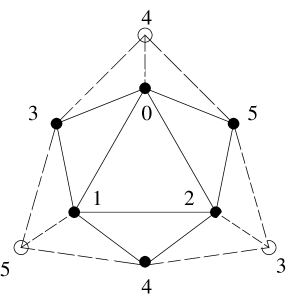
Figure 5: The minimal discretisation of $\R P^{2}$ and its geodesics. It is obtained by discretizing the points on the sphere by the vertices of an embedded icosahedron. We have to imagine that we look at the icosahedron facing one of its triangles head–on. The “sphere” is completed by identifying opposite points. Where necessary to identify all geodesics, points of the lower “half–sphere” have been drawn, connected by dashed lines. Every point can be connected with any other point by exactly one of the links, so that the geodesic rule is unique. The non–contractible paths are the ones that go along an odd number of broken lines, because broken lines lead onto the other half–sphere.

The uniqueness of the geodesic rule and the definitions of non–contractible paths on this discretisation of $\R P^{2}$ are both immediately obvious from Fig. 5. Non–contractible paths are those which follow an odd number of those links which cross the equator. Flux conservation is easily established, too: every tetrahedron edge has either one of the broken lines associated with it (i.e. it carries the field values into the other half–sphere), or a solid line. Changing any one of the links with respect to this behaviour changes the flux in two triangles. Thus, the total flux can only be changed in steps of two (or zero), and the number of triangles having strings going through them is always even. By going through the different combinations, it is easy to convince oneself that the thus constructed strings are also self–avoiding, i.e. that no tetrahedron has four faces penetrated by strings.

In the continuous case, the geodesic rule can be realised as follows: Let the random field assignment on a spatial vertex be a random vector of the upper unit half–sphere. If the vacuum manifold ${\cal M}$ were to be this half–sphere only, the length of the geodesic between two points on ${\cal M}$ would just be the angle between the two corresponding vectors. If ${\cal M}=$$\R P^{2}$, the geodesic is therefore either this angle or its complement, whatever is smaller (the probability that a pair of points is connected by a geodesic of length exactly $\pi/2$ is zero). Whenever we need to take the complement of the angle between the two vectors on the upper half sphere, the geodesic will therefore cross the equator. This happens if the two field angles have a dot product smaller than zero. Since there are three vertices to each face of the tetrahedra on our lattice, we need to take all three pairwise dot products. If the curve drawn by the geodesics has crossed the equator an even number of times, then it is contractible, otherwise a string has to pass through the corresponding triangle. Therefore, if the field values on the vertices of a particular triangle are (in the “vector on the upper half–sphere” representation) the vectors $\vec{v}_{i}\,\,,\,\,i=1,2,3$, then the string flux through the appropriate triangle is $n=\frac{1}{2}\left[1-{\rm sign}[(\vec{v}_{1}\cdot\vec{v}_{2})\,(\vec{v}_{2}\cdot\vec{v}_{3})\,(\vec{v}_{1}\cdot\vec{v}_{3})]\right]$. It cannot have negative sign, because $\R P^{2}$ strings are non–orientable. Flux conservation is easily proved [17], but a continuous representation of the $\R P^{2}$ symmetry suffers from the same uniqueness problems as a $U(1)$ string on a cubic lattice, because a single tetrahedron can carry two strings. To avoid random matching of open string segment (which might introduce an unnatural bias towards Brownian statistics on large scales [4]), we chose to connect the free ends in such a way that, in case of ambiguities, every string goes through a pair of faces which share an edge of length $a$, i.e. the edge length of the bcc lattice. The measured ensembles of $\R P^{2}$ strings are listed in Table 5.

	Number of strings	cutoff $\Lambda$	fractal dimension $D$	$b$
continuous	3000	100,000	$1.979\pm 0.023$	$2.59\pm 0.05$
	100,000	2000	$1.971\pm 0.001$	$2.643\pm 0.014$
discrete	10,000	10,000	$1.975\pm 0.014$	$2.62\pm 0.03$

Table 5: Measurements for the fractal dimension of continuous $\R P^{2}$ strings.

The continuous $\R P^{2}$ strings do not seem any more Brownian than the ones which are forced to be self–avoiding. This may indicate (as in the case of $U(1)$) that the discretisation of the vacuum manifold does not significantly affect the measurements for perfect symmetry, maybe because we have not allowed random reassignments of string pairs to each other, but we have not checked whether a random solution to the problem of uniqueness would indeed bias the statistics towards Brownian configurations. In any case, no discretisations of $\R P^{2}$, other than the minimal one, have been investigated at this stage. In fact, no discretisation which would be finer than the minimal one, but still force self–avoidance, is known to us. Interestingly enough, a discretisation produced by embedding a tetrakaidekahedron into the two–sphere is uniform. Uniform distribution of the lattice points on the sphere is a necessary criterion for unbiased data (cf. the discussion in the following sections). However, it is easy to convince oneself that many of the vector pairs in that scheme are at right angles to each other, introducing ambiguities in the definition of the string flux through a triangle. Another discretisation, achieved by embedding a dodecahedron in the sphere, produces a discretisation which does not exhibit these ambiguities, but does allow two strings to penetrate a tetrahedron. The appropriate proof is developed in the Appendix.

We should mention that $SO(3)$ strings have been measured to have a similar tendency to have lower fractal dimension, and therefore higher values for $b$. Kibble [30] arrives at values of $D=1.950\pm 0.037$, and $b=2.546\pm 0.065$. It is therefore possible that such deviations are generic for either ₂ strings or for higher dimensional vacuum manifolds. We will further discuss this issue later.

3 String Percolation and Biased Symmetry Breaking

3.1 Low String Density

Drawing lessons from polymer statistics, the fact that our algorithm generates nearly Brownian strings could be a result of the dense packing of strings. From what we have measured so far, there is a strong caveat to that statement: The continuous $\R P^{2}$ strings are actually denser ($1/\pi$ strings per face [3]) than the continuous $U(1)$ strings ($1/4$), but exhibit more “self–avoiding” statistics. This trend also holds for the minimally discretised ensembles ($5/18$ for $\R P^{2}$, and $2/9$ for $U(1)$). So how does the string density affect string statistics?

We have already shown that for minimally discretised $U(1)$-strings, a Hagedorn-like transition [31, 32, 33] occurs below a critical string density [4]. According to Vachaspati [3], we can achieve variations in the string density by inducing correlations in the order parameter by lifting the degeneracy of the manifold of equilibrium states. This reduces the probability of a string penetrating the face of a lattice (Thus we can generate an ensemble with the average  string density fixed at will. Physically one can think of this as applying an external field, which spoils the symmetry of possible ground states), but increases the dimension $D$, which argues against the identification of strings with polymers. There is a critical density below which there are no “infinite” strings. In the low density phase there is a scale $c$ which appears in the loop length distribution,

$$dn=al^{-b}e^{-cl}dl\,\,\,\,\,,\,\,\,\,\,$$ (9)

as a cut-off. As the critical density is approached from below, $c\to 0$, and the mean square fluctuation in the loop length

$$S=\langle l^{2}\rangle-\langle l\rangle^{2}\,\,\,\,\,,\,\,\,\,\,$$ (10)

diverges (see exponents $\gamma$ and $\psi$ in Table 7).

This divergence signals a phase transition, in some ways analogous to the Hagedorn transition in relativistic string theory at finite temperature. This has been implicated in many branches of physics. Previous studies [34] deal with string dynamics and can treat the ensemble in thermal equilibrium . Vachaspati’s algorithm enables us to measure directly the string statistics such as the critical density, the dimension, and the critical exponents, and to test the validity of the hypothesis of scale invariance for the initial conditions, which cannot be expected to be thermalised.

3.2 Low String density and the Hagedorn transition

From the “microscopic” point of view, Vachaspati [3] argued for such a Hagedorn-type transition to occur at low string densities with the following reasoning: consider a string formation simulation on a cubic lattice. The probability of a string passing through a certain face 1 of the cell is $p_{s}$. Since the plaquette opposite face 1 is causally disconnected, the probability for it to have a string passing through it is also $p_{s}$, regardless of the actual situation at face 1. Therefore, the probability for a string to bend after entering a cell is $1-p_{s}$. Now, if we reduce $p_{s}$, the bending probability increases and the chances of the string closing up to form a loop also increases. As Vachaspati argues, “This tells us that by reducing the probability of string formation, or equivalently, by decreasing the string density, we can decrease the infinite string density and increase the loop density”.

Vachaspati then goes on to construct a model with ₂ strings (i.e. non–orientable strings), in which he assigns either $+1$ with the probability $1-p$ or $-1$ with probability $p$ to each link of the lattice (on a periodic lattice). A string is said to pass through a plaquette if the product of the field values on the associated links is $-1$. This is, although reminiscent of it, not quite identical with the way we constructed our $\R P^{2}$ strings in the previous section, because whether a $+1$ or a $-1$ is “assigned” to a link in the continuous $\R P^{2}$ case depends on the relative angles between the three vectors involved, so that the assignment to the links are not entirely uncorrelated. If they were, then the probability of an $\R P^{2}$ string passing through a triangular (or in fact any) plaquette should be $\frac{1}{2}$, whereas it is (for a triangular plaquette and continuous $\R P^{2}$) $\frac{1}{\pi}$ [3]. The way strings are constructed in ref. [3] is, however, appropriate to model $\R P^{\infty}$ strings. We can see this by the following argument: it is well known that the different components of a random unit vector in ^N, in the limit $N\rightarrow\infty$, become mutually uncorrelated Gaussian random variables with standard deviation $\sigma=\sqrt{N}$. Any two random unit vectors will therefore have positive or negative sign with equal probability. The relative angles to a third unit vector, and in particular their signs, are then completely uncorrelated to this angle, so that taking the sign of the product of uncorrelated Gaussian random variables would indicate whether a sequence of geodesics between random points on $S^{\infty}/{}_{2}$ will cross the horizon or not.

With this model Vachaspati observed that, as the symmetry bias is increased, a lot of string mass is transferred from infinite strings to loops, so that the loop density actually increases. This is not what one would e.g. expect from statistical arguments for a box of (non–interacting) strings in equilibrium [33], so that one should not assume a priori that the string statistics right at the phase transition will follow statistical mechanics arguments. Another prediction of statistical mechanics arguments is that, at low densities, the loop distribution is described by Eq. (9), with $b=\frac{5}{2}$. Vachaspati, however, measures values consistent with 2 (within large statistical errors). As one increases the string density again, approaching the scaling regime, $c$ approaches zero from above, signalling a phase transition ($c$ can be interpreted as the inverse of some characteristic length scale arising from the breakdown of scale-invariance).

Vachaspati’s argument, relating the probability of a string forming at a particular lattice plaquette to the Hagedorn transition, actually does not go far enough: it supports a notion that the string is getting wigglier as we decrease the density, which could, strictly speaking, result in just a rescaling of some of the parameters, but none of the exponents: the scaling function in Eq. (2) could converge towards a different constant, the factor $q$ in Eq. (6) could change, all without changing $D$ or $b$, which determine the global properties of the network after the local properties have been absorbed into appropriate prefactors. In particular, the complete disappearance of infinite strings is not explained convincingly. What Vachaspati observes in Monte Carlo measurements, however, can be explained on the “microscopic” level. Vachaspati varies the string density by decreasing $p$, the probability for a link to have the value $-1$ assigned to it. Let us take it to the extreme and assume that all the links that have $-1$ assigned to them are so rare that they are usually isolated from each other, submerged into a sea of links with field value $+1$. Then it is obvious that a string loop of minimal length winds around each of these links, so that there will be nothing but a few isolated short string loops. We can take it further and ask ourselves what happens when two such links are adjacent to each other. If they are consecutive links with the same orientation, they will have their own loops of length four, if they are in different spatial orientations, a loop of length 6 will form, as depicted in Fig. 6.

 

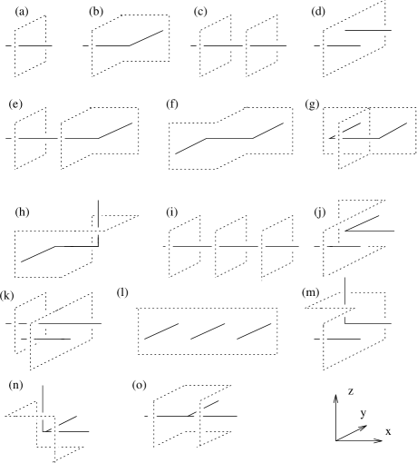
Figure 6: The string loops formed in this model, with one isolated link with field value $-1$ (a), and with two ((b) to (d)) or three ((e) to (o)) such links adjacent to each other. The fact that infinite strings disappear looks very reminiscent of a bond percolation problem for the “$(-1)$–links”, except that two consecutive strings, if they are aligned, do not surround themselves with pieces of the same string (the prototype is (c), other examples are (e), (i), and (k)), whereas neighbouring parallel links do (the prototype is now (d), with other examples being (j), (k), (l), and (m)).

This figure also illustrates that, because the length of the strings seems to be intimately linked to the size of the $(-1)$–link clusters, in the Vachaspati model, the Hagedorn transition is almost a bond percolation problem, except that parallel bonds touching each other (i.e. bonds along the same line) do not connect their strings with each other, and parallel bonds which are just one lattice spacing apart, do. There are more configurations of these “$-1$–links” that break this correspondence between the Vachaspati model and bond percolation (e.g. a flat cross of four $(-1)$–links produces two separate loops). Thus, although there is no one–to–one correspondence, one still intuitively expects the Hagedorn threshold to be close to the bond percolation threshold. Indeed, Vachaspati measures a percolation threshold of $p_{c}\approx 0.29$, while the threshold for bond percolation on a simple cubic lattice in three dimensions is $p_{c}=0.3116$ [35]. There is more to be learned from the correspondence of the Vachaspati model with bond percolation. To get a respectable number of large, but isolated lattice animals, we have to approach the percolation threshold from below. At the threshold, the percolating cluster has a well defined fractal dimension. Thus we conclude that scaling must be restored as the percolation threshold is approached from below, and a fractal dimension will begin to become well defined. Lastly, we shall just mention that one can easily derive the general form of Eq. (9) by similar percolation arguments.

Not only can we now claim to understand the microscopic aspects of the lattice description of this Hagedorn-like transition, but we also expect this transition to have many properties of a percolation transition. We can relate many variables and critical exponents of the Hagedorn transition to critical behaviour in standard percolation transitions. With his model, Vachaspati got qualitative indications of a lot of the results which are to follow here. With the infinite–lattice and the hash–table algorithms used in [4] and presented in [17, 10] we have some advantage when extracting numerical data or attempting reasonably large ensembles for good statistics.

3.3 String Percolation in the Vachaspati–Vilenkin Algorithm

Now we need to go back to the more realistic model: the Vachaspati–Vilenkin method on a tetrahedral lattice. The string density can only be varied (once the lattice is chosen) by lifting the degeneracy in the vacuum states, i.e. by making some vacuum states less likely than others. Once the details of the discretisation of space and of the vacuum manifold are chosen, the initial string density, and in particular the density in infinite strings, can only be changed by spoiling the vacuum symmetry. Some of the recent work on dynamical scaling in string networks [9] implies that the ratio of the densities in string loops and in infinite strings may be freely variable, based on the realisation that this ratio depends on the lattice description invoked. Whereas we agree with the general argument, we will show in section 6.1 that there is probably a lower limit to the amount of infinite string that has to appear, and that infinite strings would therefore be a generic feature of the VV algorithm on a regular lattice. This issue is still controversial, but in some simple cases, like the Vachaspati model, we can develop a percolation theory understanding for the emergence of an infinite string network. Had Vachaspati used a tetrahedral lattice, there would still be infinite strings, as the bond percolation problem threshold for the bcc lattice is $p_{c}=0.1803$, and the symmetric case has $p=0.5>p_{c}$. In fact, on any three dimensional lattice $p_{c}<0.5$, so that the appearance of infinite strings is lattice–independent. Serious lattice ambiguities would only arise if strings (under the same physical conditions) percolate on one lattice, but not on another, i.e. if $p_{c}$ lies in between percolation thresholds of different lattices. No such model is known.

Because of its better correspondence to a physical situation, let us consider another brief example, taken from the measurements in the next section: Take the tetrahedral lattice with a minimal discretisation of $U(1)$. Let us denote the three possible field values by 0, 1, and 2. We introduce a bias in the symmetry, such that the value 2 is assigned with the probability $p_{s}$, and the other two values have the probabilities $(1-p_{s})/2$. Without loss of generality, let us constrain ourselves to biases with $p_{s}\leq\frac{1}{3}$. We can produce infinite strings only if all three field values percolate. In particular, this implies that $p_{s}>p_{c}$, where the critical value $p_{c}$ is the site percolation threshold of a bcc lattice, $p_{s}\approx 0.246$ [35]. In the unbiased case $p_{s}=\frac{1}{3}$. Again, this is higher than the site percolation on any sensible lattice, such that the appearance of infinite strings is a generic feature. From measurements in the next section, we deduce $p_{c}=0.2476\pm 0.0014$. The agreement is almost suspiciously good, but certainly justifies the percolation theory arguments for an intuitive understanding of the Hagedorn transition. Had we taken a simple cubic lattice, we would still be above the percolation threshold $p_{c}=0.3116$, and get infinite strings [18]. In both, Vachaspati’s ₂ model and the minimally discretised $U(1)$ model we get infinite strings irrespective of the lattice we are using. Percolation phenomena have long been know to be independent of the microscopic details of the lattice. This may lend some support to the assumption that, in the Vachaspati’s ₂ model (and maybe more generally for ₂ strings) and for $U(1)$ strings the emergence of a network of infinite strings is a generic feature. Although the correspondence of the Hagedorn transition to a percolation phenomenon seems rather strong, we suffer from the same deficiency here as most of percolation theory does: there is no analytic proof.

In many respects, the best we can hope for is to establish a better understanding through better and more numerical measurements. The next section is therefore dedicated to the results of various measurables of the percolation transition. We will bring more arguments for the correspondence of the string ensembles with a percolation theory picture later when we discuss the results of those measurements.

4 Numerical Results for Biased String Formation

4.1 $U(1)$ strings

The following convention has been used to introduce a bias for $U(1)$ strings: We discretised the $U(1)$ manifold by $N=2^{n}-1$ points, and assigned the following probabilities to the each of these points $m\in\{0,1,2,...,N-1\}$

$$p(m)=C^{-1}\exp(-\eta\,\cos(2\pi m/N))\,\,\,\,\,,\,\,\,\,\,$$ (11)

where $\eta$ is the bias parameter and $C$ simply normalizes the probabilities

$$C=\sum_{m=0}^{N-1}\exp(-\eta\,\cos(2\pi m/N))\,\,\,\,\,.\,\,\,\,\,$$ (12)

Unless stated otherwise, we will quote results from the minimal discretization of $U(1)$ in this section, i.e. $N=3$. The reason why this is the best–studied ensemble is the fact that it corresponds most closely to a site percolation problem, and therefore relates best to the discussion of the results in the next section. Firstly, we confirm that Eq. (9) gives an extremely good fit for the loop distribution beyond the percolation threshold. Typical such fits are shown in Fig. 7.

 
 

Figure 7: Typical fits to the Eq. (9), with different values of the bias. Where infinite strings are present, no cutoff can be identified. Where $\Lambda<1/c$ (i.e. for $\eta=0.4$), the cutoff cannot be seen, as the strings in this ensemble are too short. For higher values of the bias, the cutoff can be recognised clearly. The dashed lines are the fits using Eq. (9). No deviations from a behaviour of the type in Eq. (9) can be recognised. The ensemble consists of 100,000 strings with cutoff $\Lambda=2000$.

In Fig. 8 we compare the loop distributions for different biases. It can be seen that for low bias the string density in loops increases with increasing bias, in agreement with Vachaspati’s measurements.

 

Figure 8: Comparison of the loop distributions for different bias. It can be seen that the loop density is increased for small bias. For large bias, the running of the cutoff length can be observed.

The density in loops as a function of $\eta$ is shown in Fig. 9. The mass density in loops (in units of segments per tetrahedron) is obtained in the following way: Let $p_{t}$ be the probability for a triangle to carry a string segment. Since the number of triangular plaquettes on a tetrahedral lattice is twice the number of tetrahedra, the average number of strings per tetrahedron is then $2p_{t}$. Whenever we start tracing a string, we start at a randomly chosen string segment (out of all possible segments on the imagined infinite lattice). Thus we will pick elements belonging to an infinite string according to their density ratios, such that

$$\rho_{\rm loop}=\rho_{\rm total}\,\frac{N_{\rm loop}}{N_{\rm total}}\,\,\,\,\,,\,\,\,\,\,$$ (13)

where $N_{\rm total}$ is the number of strings we have traced in the ensemble, and $N_{\rm loop}$ is the number of those which turned out to be loops. The unknown parameter is $p_{t}$. For the minimally discretised $U(1)$ manifold, the sum $C$ of Eq. (12) is just

$$C=2\,e^{\frac{\eta}{2}}+e^{-\eta}\,\,\,\,\,,\,\,\,\,\,$$ (14)

and the probability for a triangle to exhibit all three vacuum values on its vertices reduces to the very simple form

$$p_{t}=\frac{3!}{C^{3}}\,\,\,\,\,.\,\,\,\,\,$$ (15)

For other discretisations of $U(1)$ we use exact numerical summations to extract $p_{t}$, as the functional form becomes a rather complicated sum of a number of terms that increases as $N^{3}$ and has to be evaluated for all values of $\eta$ used in the data set. It turns out that the defect density increases slightly when a finer discretisation of the vacuum manifold is used. The string density per tetrahedron in terms of the bias, for the minimal discretisation of $U(1)$, is therefore given by

$$\rho_{\rm total}=\frac{2\cdot 3!}{(2e^{\frac{\eta}{2}}+e^{-\eta})^{3}}\,\,\,\,\,.\,\,\,\,\,$$ (16)

This can be used as a reparameterisation of the bias, so that all variables $X$ scaling like $X\propto|\eta-\eta^{\star}|^{\chi}$ near the critical point will also scale as $X\propto|\rho_{\rm total}-\rho_{\rm total}^{\star}|^{\chi}$, as it is a smooth and analytic function of the bias. Fig. 9 shows the separate mass densities in infinite strings and loops. Note that the energy in loops at the percolation transition

 

Figure 9: The mass density in string segments belonging to loops (in units of one per tetrahedron) (solid line), in infinite strings (dashed line), and the total mass density, given by Eqs. (13) and (15). The loop density increases as we approach the percolation threshold from above, and energy from infinite string is transferred into the loop ensemble.

still exceeds the energy in infinite string at zero bias! In analogy with the polymer literature, we could say that this transition (when approached from the non–percolating phase) is very efficient in pumping energy into the entropy terms, i.e. in utilising new degrees of freedom as the bias is lowered.

Figure 9 allows us to measure the location of the percolation threshold, by fitting a power law of the form

$$\rho_{\infty}\propto(\eta^{\star}-\eta)^{\beta}\,\,\,\,\,.\,\,\,\,\,$$ (17)

We do this by trying different fixed values of $\eta^{\star}$ and taking the one that gives the smallest sum of residuals on a log–log least squares fit. We measure

$$\beta=0.54\pm 0.10\,\,\,\,\,,\,\,\,\,\,$$ (18)

where the fit has been done in the region $\eta\in[0.22,0.265]$, and the errors are associated with the uncertainty in $\eta^{\star}$, which is measured to give the best fit at $\eta^{\star}=0.279\pm 0.005$. If the uncertainty in $\eta^{\star}$ is large, the errors for $\beta$ get quickly out of hand. The criterion of whether one gets a good fit or not is not very efficient in finding $\eta^{\star}$, but it is the best we can do.

The fractal dimension is plotted in Fig. 10 for nearly continuous $U(1)$, but with different upper cutoffs $\Lambda$, and in Fig. 11 for $\Lambda=50,000$, but with different discretisations of $U(1)$. Five features are noteworthy:

• The statistical errors increase with increasing bias, because the number of infinite strings in the ensemble becomes smaller.

• The fractal dimension stays nearly constant for very small bias. We observe that the $\Lambda$–dependence of $D$ as measured in the previous section is not a statistical fluctuation.

• The fractal dimension becomes not only hard to measure near the percolation threshold, but also becomes ill–defined beyond it, because we are counting many strings wrongly as infinite ($\langle l_{\rm loop}\rangle$ diverges at the critical point), whereas they will eventually turn back onto themselves and form loops.

• The behaviour is largely independent of the particular discretisation used, except for the obvious shift in $\eta^{\star}$, pronounced only for $N=3$.

• The measurements are consistent with a possible assumption that, as $\Lambda\rightarrow\infty$, $D=2$ right up to the critical point.

 

Figure 10: The fractal dimension of the infinite string ensemble as a function of the bias, plotted for different values of the upper length cutoff $\Lambda$. The measurements are for nearly continuous $U(1)$.

 

Figure 11: The fractal dimension of the infinite string ensemble as a function of the bias parameter, plotted for different discretisations of $U(1)$. The critical biases can be found in Table 7 and in Figure 17.

Measurements for the average loop size are shown in Figs. 12 and 13. In Fig. 13 the effects of a finite cutoff are also explained.

 

Figure 12: The average length of a loop in the minimal discretisation of $U(1)$, as a function of the bias $\eta$. Here $\Lambda=50,000$.

 

Figure 13: The logarithm of the average length of a loop (with $U(1)$ nearly continuous: $N=255$, and $N=127$) as a function of the bias $\eta$, for different cutoffs. For the solid line $\Lambda=1,000,000$, whereas for the dashed line it is $\Lambda=50,000$. They should (to very good approximation) have the same critical bias. However, the lower–cutoff peak has an inflexion point, where it deviates from the power–law behaviour, well before the critical point (at around $\eta=0.36$), where we need to stop the fits to measure the critical exponents. This effect gets worse with smaller cutoffs, and gives rise to inaccuracies in estimating the exact position of $\eta^{\star}$.

The behaviour is just as one would expect from percolation theory: In the non–percolating phase, the main contribution comes from gradually larger clusters as we approach the percolation threshold.

Let us assume the average loop size near the percolation threshold scales as

$$\langle l_{\rm loop}\rangle\propto|\eta-\eta^{\star}|^{-\gamma}\,\,\,\,\,.\,\,\,\,\,$$

The best power–law fits to the loop size give

$$\eta^{\star}_{(N=3)}=0.279\pm 0.004\,\,\,\,\,,\,\,\,\,\,\gamma=1.59\pm 0.10\,\,\,\,\,,\,\,\,\,\,$$

measured in the range $\eta\in[0.33,0.6]$. Again, large errors are associated with the uncertainty of where exactly the percolation threshold lies.

For bias values below the percolation threshold there is no critical exponent. In this domain the average loop length is a divergent function of the upper cutoff, and an average length becomes ill–defined. This is obvious from Eqs. 4 and 5 and the fact that $\langle l_{\rm loop}\rangle\propto\int_{\lambda}^{\Lambda}l^{-b+2}\,dl$ while $D>3/2$. This problem is alleviated in the non–percolating regime (where the loop distribution is exponentially suppressed by an additional factor of $e^{-cl}$), as long as $\xi=1/c\ll\Lambda$, i.e. for values of $\eta$ not too close to the critical bias. The same argument holds for any higher moment $\langle l_{\rm loop}^{n}\rangle$ of the loop distribution.

Another way of investigating the ensemble is by means of a partition function, which is the (un–normalized) sum over probabilities $p(l)$

$$Z=\sum_{l}l^{-b+1}e^{-cl}\,\,\,\,\,.\,\,\,\,\,$$ (19)

This is not a thermal partition function, but should rather be viewed as a generating function for the moments of the loop size distribution. If we wanted to use thermodynamics language, then the factor $l^{-b+1}$ would be proportional to the density of states for given $l$ (or one could say it is a suitably defined integration measure, which amounts to the same), and $\xi=1/c$ fulfils the role of a temperature, as is shown in the Appendix. This only serves to show that a thermodynamic nomenclature is inappropriate, as the threshold for a dynamical Hagedorn transition really lies at a finite temperature, and instead of having the temperature diverge at the critical point, one would have to factor out the divergent terms and pull them into the density of states. This distinction becomes meaningless in our non–thermal ensemble. Our “partition function” can equally well be viewed as a sum over the density of states only, with a critical temperature (or density) dependence. Although these names are slightly inappropriate, they give the right behaviour e.g. for the average energy $\langle l_{\rm loop}\rangle$ in the non–percolating phase

$$``E"=\langle l_{\rm loop}\rangle=-Z^{-1}\frac{d}{dc}{\rm ln}\,Z\,\,\,\,\,.\,\,\,\,\,$$

Since the parameters $b$ and $c$ are crucial in this interpretation, measurements for them are shown in Figs. 14 and 15.

 

Figure 14: The loop distribution exponent $b$ in Eq. (9), for an ensemble of 10,000 strings with cutoff $\Lambda=50,000$.

 

Figure 15: The parameter $c$ in Eq. (9) for the same ensemble as in Fig. 14.

Although the parameters $b$ and $c$ are comparably easy to measure, since one does not have to guess $\eta^{\star}$, there are still large statistical fluctuations for $b$. For $\eta>\eta^{\star}$, $b$ is allowed to be smaller than two, since the scaling relation Eq. (5) does no longer hold. It becomes more difficult to measure $b$ at large bias, but it is also less important there, since the exponential cutoff dominates the loop size distribution. The diverging length scale associated with the phase transition is $\xi=1/c$, which is plotted in Fig. 16.

 

Figure 16: The parameter $\xi=1/c$ in Eq. (9) for the same ensemble as in Fig. 14. Very large values in the region $\eta<\eta^{\star}$ just correspond to statistical fluctuations of $c$ around zero.

There is another critical exponent associated with the divergence of $\xi$:

$$\xi\propto(\eta-\eta^{\star})^{-\frac{1}{\sigma}}\,\,\,\,\,.\,\,\,\,\,$$

Implicitly, we measure for the percolation threshold $\eta^{\star}=0.280\pm 0.003$. The critical exponent is

$$\sigma=0.46\pm 0.02\,\,\,\,\,.\,\,\,\,\,$$ (20)

Before concluding this section, we measure the critical exponent in

$$\langle l_{\rm loop}^{2}\rangle\propto(\eta-\eta^{\star})^{-\psi}\,\,\,\,\,,\,\,\,\,\,$$

which gives (as well as $\eta^{\star}=0.277\pm 0.004$)

$$\psi=3.79\pm 0.14\,\,\,\,\,.\,\,\,\,\,$$

This is the exponent associated with what we called “susceptibility” in ref. [4], $S=\langle l_{\rm loop}^{2}\rangle-\langle l_{\rm loop}\rangle^{2}$, since the diverging behaviour of $\langle l_{\rm loop}^{2}\rangle$ dominates in the expression for $S$, because $\psi>2\gamma$. In terms of the partition function, it is

$$\langle l_{\rm loop}^{2}\rangle=Z^{-1}\frac{d^{2}}{dc^{2}}\,Z\,\,\,\,\,,\,\,\,\,\,$$

such that $\langle l_{\rm loop}^{2}\rangle=-Z^{-1}\frac{d}{dc}(Z\langle l_{\rm loop}\rangle)$. When compared to a Hagedorn transition, however, we want the derivative of $\langle l_{\rm loop}\rangle$ with respect to a temperature (i.e. any smooth reparameterisation of the bias), such that a proper definition of the susceptibility as the energy cost per loop associated with decreasing $\eta$ would simply diverge with an exponent $(-\gamma-1)$. Another reasonable definition of a susceptibility would be to define it (at least for $\eta>\eta^{\star}$) as $\frac{d}{d\eta}\rho_{\rm loop}$, which then diverges with the exponent $(-\beta-1)$.

This concludes the discussion of the critical behaviour of the ensemble with a minimal discretisation of $U(1)$. Measurements for the other ensembles with gradually finer discretisations of the vacuum manifold are listed in Table 7 . A reminder of which exponent is associated with which variable can be found in Table 6.

$\xi=1/c\propto(\eta-\eta^{\star})^{-\frac{1}{\sigma}}$

$\langle l_{\rm loop}\rangle\propto(\eta-\eta^{\star})^{-\gamma}$

$\langle l_{\rm loop}^{2}\rangle\propto(\eta-\eta^{\star})^{-\psi}$

$\langle\rho_{\infty}\rangle\propto(\eta^{\star}-\eta)^{\beta}$

Table 6: A summary of the definition of the critical exponents.

N	$\Lambda$	$\eta^{\star}$	$\sigma$	$\gamma$	$\psi$	$\beta$
3	50,000	$0.279\pm 0.005$	$0.46\pm 0.02$	$1.59\pm 0.10$	$3.79\pm 0.14$	$0.54\pm 0.10$
7	50,000	$0.299\pm 0.005$	$0.44\pm 0.02$	$1.77\pm 0.14$	$3.85\pm 0.16$	$0.45\pm 0.07$
15	50,000	$0.295\pm 0.007$	$0.39\pm 0.04$	$1.86\pm 0.13$	$4.5\pm 0.3$	$0.39\pm 0.06$
31	50,000	$0.305\pm 0.005$	$0.42\pm 0.02$	$1.75\pm 0.03$	$4.1\pm 0.3$	$0.45\pm 0.06$
63	50,000	$0.309\pm 0.005$	$0.417\pm 0.017$	$1.69\pm 0.07$	$4.0\pm 0.2$	$0.50\pm 0.07$
127	50,000	$0.301\pm 0.004$	$0.413\pm 0.013$	$1.80\pm 0.06$	$4.07\pm 0.14$	$0.41\pm 0.05$
255	2,000		$0.339\pm 0.005$	N/A	N/A	N/A
255	$10^{6}$	$0.300\pm 0.002$	N/A	$1.83\pm 0.07$	$4.10\pm 0.15$	$0.456\pm 0.025$

Table 7: The critical exponents and percolation thresholds for different discretisations of $U(1)$. The values quoted for $\eta^{\star}$ are taken from the measurement of $\gamma$. In the case of the very low $\Lambda$, the divergences for loop sizes flatten out long before the critical point, and no exponents can be extracted. For very large $\Lambda$, however, the number of traced strings is not large enough to extract $c$. The errors quoted are statistical errors only.

Ideally, we should have two ensembles for every discretisation, one with a small $\Lambda$, allowing us to trace a larger number of strings to extract the exponent $c$, and one with very large $\Lambda$, to measure the divergences in the average loop size, to which the loops of length $l\stackrel{{\scriptstyle<}}{{\sim}}\Lambda$ contribute the most, as we approach the critical point. However, we do not notice too much of a reduction of statistical errors by doing this (as is done for $N=255$), so these ensembles have not been generated. A cutoff of $\Lambda=2,000$ is clearly too low to give sensible answers.

Another consequence of finite cutoff effects is that the measurements of $\gamma$ give the best fits to a power law and are therefore the best indicators of where the percolation threshold lies. The reason for this is simple to understand: large loops give the main contribution towards the length average, and finite cutoff effects will eventually flatten the peak which should diverge at the critical bias. However, the contribution of large loops to $\langle l_{\rm loop}^{2}\rangle$ is even more important, and finite cutoff effects will spoil the power law approach to the critical point at a much earlier stage, such that $\psi$ has much larger errors associated with it, and it is recommendable to use estimates for $\eta^{\star}$ which were obtained from fits of the average loop size to a power law behaviour. The same is true for $c$ (and its associated exponent $\sigma$), because of similar reasons, which, in an intuitive fashion one might simply sum up as: the smaller the modulus of the critical exponent, the closer one can go towards the critical point without feeling finite size effects.

In Fig. 17 we present the values of the critical string density as a function of the discretisation of $U(1)$. It can be seen that $N\stackrel{{\scriptstyle>}}{{\sim}}15$ is already very close to the continuous $U(1)$ limit. In this sense, the ensembles with $N\geq 31$ in Table 7 can be interpreted as the same measurements over several ensembles of the same kind.

 

Figure 17: The critical string density (in units of string segments per tetrahedron) plotted against the number of discretisation points for the $U(1)$ manifold.

Lastly, it is worthwhile testing the validity of the scaling relation for configurational exponents, Eq. (5), which – as we have discussed before – implies that on intermediate scales loops show the same fractal behaviour as infinite strings. Scaling seems to hold roughly. Considering that the exponent $b$ is usually taken from quite noisy data (except when close to the percolation threshold), the agreement seems very good, and is shown in Fig. 18 for the $N=63$ ensemble. When $c$ is constrained to be zero, as it was done to obtain Fig. 18, such plots give a very good first estimate of the percolation threshold and the Fisher exponent $\tau$, i.e. the value of $b$ at criticality, which plays a prominent role in the next section, when we will come to use the partition function to describe general scaling relations.

 

Figure 18: Testing the validity of Eq. (5) on a $U(1)$ string ensemble with $N=63$.

4.2 $\R P^{2}$ strings

For $\R P^{2}$ strings our conventions of what the bias means depend on the discretisation. For the minimally discretised $\R P^{2}$ strings (cf. Fig. 5), we define a bias $\zeta$ as:

$$p(0)=p(1)=p(2)=\frac{1+\zeta}{6}\,\,\,\,\,,\,\,\,\,\,p(3)=p(4)=p(5)=\frac{1-\zeta}{6}\,\,\,\,\,,\,\,\,\,\,$$ (21)

such that $\zeta=1$ corresponds to $\rho_{\rm total}=0$, $\zeta=0$ is a perfect $\R P^{2}$ symmetry, and $\zeta=-1$ a perfect $U(1)$. For the continuous $\R P^{2}$ simulations, we define a bias $\mu$ such that the normalized probability density for the polar angle $\theta\in[0,\pi/2)$ (i.e. constrained to the upper half–sphere) is

$$d\,p(\theta)=\frac{\mu}{1-e^{-\mu}}e^{-\mu\,\cos\theta}\sin\theta d\theta\,\,\,\,\,.\,\,\,\,\,$$ (22)

The unbiased case corresponds again to $\mu=0$, but $\mu$ can run from $-\infty$ to $\infty$, where it corresponds to zero string density or a $U(1)/{}_{2}$ symmetry, respectively.

Apart from the critical exponents, the interesting feature about biased $\R P^{2}$ symmetries is that one can bias them towards the $U(1)$ ensembles which we have measured already. The fractal dimension then runs from what we have measured for $U(1)$ to values lower than two. This is shown in Fig. 19.

 

Figure 19: The running of the fractal dimension. At zero bias we measure $D=1.96$, whereas for large positive bias the $U(1)$ measurements are recovered asymptotically. As we approach the zero–density limit (large negative $\mu$), the fractal dimension increases sharply before becoming ill–defined. The ensemble has 3,000 strings with $\Lambda=10^{5}$.

If this effect is caused by the running of the string density, as comparisons of the relative densities seem to suggest (the average number of penetrated triangles in continuous $U(1)$ is $\frac{1}{4}$, whereas for continuous $\R P^{2}$ it is $\frac{1}{\pi}$ [3]), our case for arguing that the string statistics quite generally depend on the string density in a way opposed to the tendency polymers show, gets further support from this picture. Vachaspati’s model itself would be the obvious testing ground for such a hypothesis (the penetration probability per plaquette is $\frac{1}{2}$, the highest known in any model so far), but unfortunately he quotes neither measurements for $D$ nor for $b$ at zero bias, and his plots have too large statistical fluctuations to extrapolate towards zero bias. A more detailed analysis of this is given later, in Fig. 22.

Let us now turn to the measurements of the critical exponents. The average loop size has a very distinct peak at the critical point, immediately allowing a rough estimate of the critical bias at $\mu^{\star}=-1.875\pm 0.025$. This is displayed in Fig. 20.

 

Figure 20: The loop size distribution for negative $\mu$ only. It allows a very good estimate of the position of $\mu^{\star}$.

When we measure $\gamma$, we get the best fits for $\mu^{\star}=-1.86\pm 0.01$, and

$$\gamma=1.70\pm 0.06\,\,\,\,\,,\,\,\,\,\,$$

seemingly in very good agreement with the $U(1)$ data. Also

$$\psi=3.83\pm 0.14\,\,\,\,\,,\,\,\,\,\,\sigma=0.435\pm 0.013\,\,\,\,\,.\,\,\,\,\,$$

To obtain $\langle\rho_{\infty}\rangle$, we first calculate $\rho_{\rm total}$ with a Monte Carlo integration

$$\rho_{\rm total}=\int\int\int d\Omega_{1}\,d\Omega_{2}\,d\Omega_{3}\,n\,p(\Omega_{1})\,p(\Omega_{2})\,p(\Omega_{3})\,\,\,\,\,,\,\,\,\,\,$$

where $\int\,d\Omega$ stands for $\int_{0}^{2\pi}\,d\phi\,\int_{0}^{\pi/2}\,d\theta$, $p$ is defined by Eq. (22), and $n$ is the string flux as a function of the three pairwise dot products, as defined in the previous section. Then we take again $\rho_{\infty}=\rho_{\rm total}\,\frac{N_{\infty}}{N_{\rm total}}$, where $N$ with a subscript stands simply for the total number of appropriate strings in the ensemble. The results of this integration are plotted in Fig. 21, together with the mass density in loops and infinite strings.

 

Figure 21: The density of string segments in the continuous $\R P^{2}$ ensembles as a function of bias. The density in loops is shown as the dot–dashed line, and the density in infinite strings is the dashed line.

It can be seen that the loop density is considerably lower than for $U(1)$, climbing toward the value measured for $U(1)$ strings as $\mu\rightarrow\infty$, and making up the total string density beyond the percolation threshold. There are some statistical errors attached to the lines indicating the loop and infinite string density, as the ensemble of Fig. 21 consists of only 3000 strings ($\Lambda$=100,000).

From the infinite string density we measure

$$\beta=0.40\pm 0.03\,\,\,\,\,.\,\,\,\,\,$$

A comprehensive table of measurements can be found in Table 8.

Let us now come back to a question raised earlier: is the string density the fundamental parameter, dictating $D$ and $b$? Fig. 22 shows that this cannot be the case. There we plot the density vs. the fractal dimension. Most of the density regime is reached twice, once for negative $\mu$ and once for positive $\mu$. The fractal dimension, as we go towards the critical point, diverges already for string densities higher than the densities we can achieve for positive $\mu$, where the string ensemble just turns into a $U(1)$–set of Monte Carlo data. The fundamental lesson to learn from this is that, although spoiling the symmetry may be the only way to change the string density in our lattice description, it can – sometimes – be done in different ways, and lead to entirely different results.

 

Figure 22: The density of string segments in the continuous $\R P^{2}$ ensembles as a function of the total string density. The two ends of the function differ distinctly for positive and negative values of the bias.

For the minimal discretisation of $\R P^{2}$ it is straightforward but lengthy to derive

$$\rho_{\rm total}=\frac{1}{18}\left[5-3\zeta^{2}-2\zeta^{3}\right]\,\,\,\,\,.\,\,\,\,\,$$

It can be seen that it has the right behaviour $\rho_{\rm total}\rightarrow 0$, if $\zeta\rightarrow+1$ and $\rho_{\rm total}\rightarrow\frac{2}{9}$, which is the value for the minimal discretisation of $U(1)$, as $\zeta\rightarrow-1$. It also has an extremum at perfect symmetry $\zeta=0$. This means it shows all the qualitative features of the bias dependence we observed in Fig. 21 for the continuous $\R P^{2}$ strings . The density, together with the density in loops and infinite strings, is shown in Fig. 23. All components have qualitatively the same behaviour as in the continuous $\R P^{2}$ ensembles.

 

Figure 23: The string densities of the discretised $\R P^{2}$ ensembles. The contributions from loops and infinite strings are shown separately.

From this we can conclude that, again, the discretisation of the vacuum manifold does not spoil the physical picture qualitatively.

On sets of 10,000 strings with $\Lambda=$25,000, we measure that the percolation threshold is at $\zeta^{\star}=0.425\pm 0.004$, $\sigma=0.40\pm 0.03$, $\beta=0.34\pm 0.04$, $\gamma=1.68\pm 0.13$, and $\psi=3.75\pm 0.25$.

What is somewhat unexpected, is that for the $\R P^{2}$ ensemble, violation of the ‘strict’ scaling relation Eq. (5) seem to be apparent even in the regime of low bias. Where the bias turns the symmetry into $U(1)$, the strict scaling relation Eq. (5) seems to hold. For the other values, although statistical fluctuations are recognisable, there seems to be a consistent trend towards too large values for $b$, which disappears again at the critical point (cf. the same discussion for biased $U(1)$ strings). Perhaps, the deviations seen for $U(1)$ in Fig. 18 are also not just statistical errors. An analogous plot for minimally discretised $\R P^{2}$ strings is shown in Fig. 24 for the discretised manifold and in Fig. 25 for the continuous one.

 

Figure 24: The scaling relation Eq. (5) seems to be consistently violated, even in the low bias regime, except at the critical point and, perhaps, at a perfect $U(1)$ symmetry. These are the ensembles with the discretised $\R P^{2}$ manifold. The loop statistics are not extremely good, as the number of loops for zero bias (i.e. where it is the lowest) is $\approx 1800$.

 

Figure 25: The same plot as in Fig. 24 for the continuous $\R P^{2}$ manifold. There are also large statistical errors in $b$, as the number of loops is extremely small ($\approx 500$) at low bias.

The obvious source to suspect would be a cutoff–dependence for $b$. However, this is not the case. We have changed upper and lower cutoffs for the loop distribution before fitting it to Eq. (4), and the results do not change qualitatively: $b$ stays recognisably larger than predicted by Eq. (5). Clearly, a better analysis of this violation of scale-invariance, even in the percolating regime, is needed. Here, however, we will focus on the non-percolating regime from now on.

5 Percolation Theory, Universality, and Polymers

5.1 Percolation Theory and Critical Phenomena

The most notable fact about the critical exponents we have measured in the previous section is that they do not only agree with each other, thus indicating universal behaviour for string defects at the critical density, but also show reasonable agreement with the exponents obtained by standard site or bond percolation. This fact has already been noticed for the $N=3$ discretisation of $U(1)$ strings [28]. We give a comparison of the measured exponents, including their statistical errors, with known results from percolation theory in Table 8.

exponent	percolation	minimally	continuous	discrete	continuous
	theory	discretised $U(1)$	$U(1)$	$\R P^{2}$	$\R P^{2}$
$\sigma$	0.45	0.46(2)	0.42(2)	0.435(13)	0.40(3)
$\beta$	0.41	0.54(10)	0.45(3)	0.41(3)	0.34(4)
$\gamma$	1.80	1.59(10)	1.77(6)	1.70(6)	1.68(13)
$\psi$	4.04	3.79(14)	4.10(15)	3.83(14)	3.75(25)

Table 8: A summary of all the measured critical exponents, compared with critical exponents in three dimensional site (or bond) percolation.

It is seen that the continuous symmetries show some reasonable correspondence with percolation data, whereas the minimally discretised $U(1)$ ensemble deviates more strongly. The $\R P^{2}$ data has critical exponents which are consistently slightly lower than the percolation theory exponents. This allows some fairly wide–ranging conclusions. For instance, we can now – without having made the appropriate measurements – expect Vachaspati’s model not only to be “nearly” a bond percolation problem as far as the actual percolation threshold is concerned, but it may also have critical exponents very close to the ones of bond percolation

This is indeed somewhat surprising: from the point of view of percolation theory, we have constructed a very awkward definition of “clusters”. Not only are they topologically defined, but also definable through continuous, as well as discrete, manifolds of possible lattice states.

There is another comment to be made: From Table 8, one could hypothesize that there may be a trend for higher–dimensional manifolds to deviate more strongly from percolation data. However, Vachaspati’s previously discussed model describes strings produced from a $S^{\infty}/{}_{2}$ ground state manifold. We have shown above that this model corresponds closely to site percolation, such that one expects especially the Vachaspati model to be close to a percolation problem. One would therefore not expect the differences between the $\R P^{2}$ data and standard percolation exponents to be a generic consequence of the higher dimensionality of the manifold.

However, our measurements certainly do not seem to compellingly suggest exact agreement of our critical exponents with bond (or site) percolation in three dimensions. Nevertheless, the relative smallness of the deviations should make no difference when ones tries to understand the possible physical relevance of the string statistics near the critical point. Let us therefore try and learn some more lessons from percolation theory.

5.2 Fisher Exponent and Partition Function

The first step towards some indications that there are some universal relations between the configurational exponents (and that, therefore, we may extract more exponents than we have actually measured), has been done already by defining a partition function in Eq. (19), which we can view as a generating function for the loop size distribution, such that

$$\langle l_{\rm loop}^{n}\rangle=Z^{-1}\left(-\frac{d}{d\,c}\right)^{n}Z\,\,\,\,\,.\,\,\,\,\,$$ (23)

This partition function has the same functional form as the one derived in [34] in the dilute free–string approximation. If we want to get back to a physical interpretation of the partition function, it is perhaps natural to expect some of the ingredients of the results of ref. [34] to enter the description. In this way, one is led to interpret $c$ as an effective string tension $\sigma_{\rm eff}$, divided by a temperature, and the Hagedorn transition occurs when the effective string tension (or the effective energy per unit length of string) is zero. Another paper by the same authors [36] then provides the understanding for the mechanism by which the Hagedorn transition occurs in the case of biased symmetries: we have seen from the microscopic details of the lattice description that, for biased symmetries, the strings tend to become more crumpled as they wind around the sparsely spread lattice points with disfavoured vacuum values. In [36] it has been shown that for the reverse situation, when one tries to incorporate stiffness, the effective string tension for fixed temperature behaves as

$$\sigma_{\rm eff}=\sigma-\frac{{\rm ln}\left[(1+z)\,e^{-\beta\,u}\right]}{l_{o}\,\beta}\,\,\,\,\,,\,\,\,\,\,$$

where $u$ is the energy cost of turning a string through a right angle, and $z$ is the number of directions available to the string at every lattice point. From the details of the lattice description (and also from an intuitive point of view in the continuum case), this energy cost becomes negative for strongly biased symmetries, so that for some value of the bias $\sigma_{\rm eff}=0$ will be achieved, and a Hagedorn transition occurs. However, this correspondence is qualitative at best, since we do not deal with string dynamics, and the actual string tension right at the phase transition is zero by definition (at least in the case of a second–order phase transition). A more stringent proof that such a thermal interpretation of the partition function yields nonsensical results is developed in the Appendix. Since “our” partition function describes the initial conditions for dynamical calculations, one should not view it as being more than the generating function of the moments of the loop length distribution.

If we know how $b$ and $c$ scale at the critical point, we can derive the critical exponents for all the moments of the loop length distribution. From the previous section it is clear that $b$ depends only weakly on the bias, whereas $c$ scales as $c\propto|\eta-\eta^{\star}|^{-\gamma}$. In agreement with the percolation theory literature, we define $\tau=b(\eta^{\star})$ and will call it the Fisher exponent. The critical exponents for the moments of the loop distribution are then derived by

$$\langle l_{\rm loop}^{n}\rangle=Z^{-1}\left(-\frac{d}{d\,c}\right)^{n}\,\left[\sum_{l}l^{-\tau+1}e^{-cl}\right]\propto\sum_{l}l^{-\tau+1+n}e^{-cl}$$

Approximating the sum by an integral, we have

$$\langle l_{\rm loop}^{n}\rangle\propto\int l^{-\tau+1+n}e^{-cl}dl\propto c^{\tau-2-n}\int z^{2-\tau}e^{-z}dz\propto|\eta-\eta^{\star}|^{\frac{\tau-2-n}{\sigma}}\,\,\,\,\,,\,\,\,\,\,$$ (24)

where we have approximated $b$ by the constant $\tau$ in the first step, and used $c\propto|\eta-\eta^{\star}|^{1/\sigma}$ in the last step. The integral over $z$ is just a numeric constant. Thus we find that the following scaling relations should hold for our string ensembles

$$\gamma=\frac{3-\tau}{\sigma}\,\,\,\,\,,\,\,\,\,\,\psi=\frac{4-\tau}{\sigma}\,\,\,\,\,,\,\,\,\,\,$$ (25)

and so on for higher moments of the loop distribution. In this way, one can use two of the critical exponents as the fundamental ones, and derive the others from them. The fact only two critical exponents can be independent is also a consequence of the existence of just one crossover length scale. This is discussed in ref. [24]. The trouble with our definition of a generating function is that it yields the loop length distribution only for $\eta>\eta^{\star}$. What one is interested in for low bias is the density in infinite strings. The critical exponents thereof cannot be extracted as straightforwardly as the other exponents of the loop distribution, seeing that $\langle l_{\rm loop}^{0}\rangle$ would formally correspond to 1. A prescription which is generally workable in percolation theory , is to argue that, since

$$\langle l_{\rm loop}\rangle\propto\frac{d}{d\,c}\langle l_{\rm loop}^{0}\rangle\,\,\,\,\,,\,\,\,\,\,$$

we can write

$$\rho_{\infty}={\rm const_{1}}+{\rm const_{2}}\,\langle l_{\rm loop}\rangle\,c\,\,\,\,\,,\,\,\,\,\,$$

and therefore

$$\rho_{\infty}\propto|\eta-\eta^{\star}|^{\frac{\tau-3}{\sigma}+\frac{1}{\sigma}}\,\,\,\,\,,\,\,\,\,\,$$

such that we have

$$\beta=\frac{\tau-2}{\sigma}\,\,\,\,\,.\,\,\,\,\,$$ (26)

One may wonder why this gives the behaviour for infinite strings rather than the total mass density or the loop mass density. To answer this, one can just remind oneself that we have extended arguments which hold only for loops at $\eta>\eta^{\star}$. In this regime, gradually longer and longer loops dominate the loop size distribution, such that, if we extend the arguments beyond the percolation threshold, it is only the infinite strings which contribute to the moments of of this distribution .

The scaling relations (25) and (26) seem to be very well obeyed by the critical exponents we measure, and seem to give a value of $\tau$ consistent with what we observe in Fig. 18, and consistent with each other. The different predictions of $\tau$, to make the scaling relations consistent with each other, are listed in Table 9.

	minimally	continuous	discrete	continuous
	discretised $U(1)$	$U(1)$	$\R P^{2}$	$\R P^{2}$
$\tau=\beta\sigma+2$	2.25(6)	2.19(2)	2.18(2)	2.14(3)
$\tau=3-\gamma\sigma$	2.27(8)	2.26(6)	2.26(5)	2.33(11)
$\tau=4-\psi\sigma$	2.26(15)	2.28(15)	2.33(11)	2.50(22)

Table 9: Testing the scaling relations Eqs. (25) and (26) by comparing the values of the Fisher exponent predicted by them.

5.3 The Average Loop Size

Encouraged by this, we can go on to another cosmologically perhaps more relevant parameter, which is not directly measurable from our ensembles, since we did not record string–string correlation functions. It is another correlation length, call it $\chi$, which measures the average separation between two points on the same string. This gives a clearer picture of the actual physical size of a collapsed string lump beyond the percolation transition. Define

$$\chi^{2}=\frac{\sum_{r}r^{2}g(r)}{\sum_{r}g(r)}\,\,\,\,\,,\,\,\,\,\,$$

where $g(r)$ is the probability of finding, at a distance $r$ from the origin, a segment of string belonging to the same string as the segment at the origin. If we call the average squared distance between two string segments $R_{l}^{2}$, we have to weigh it with the number of string segments in loops of given length to obtain the same definition for $\chi$ in terms of $R_{l}^{2}$

$$\chi^{2}=\frac{2\sum R_{l}^{2}\,n_{l}\,l^{2-\tau}e^{-cl}}{\sum n_{l}\,l^{2-\tau}e^{-cl}}\,\,\,\,\,.\,\,\,\,\,$$

Thus, apart from numerical prefactors, $\chi$ is the radius of those loops which give the main contribution to $\langle l\rangle$. Since we have already established that, at least close to the percolation threshold, Eq. (5) is satisfied and loops have part in a proper definition of the fractal dimension, we can substitute $R_{l}\propto s^{1/D}$, and the numerator scales, according to Eq. (24), with a critical exponent $(3-\tau+2/D)/\sigma$. The denominator is just $\langle l\rangle$, such that, for the longest loops (i.e. the ones which exhibit fractal behaviour on intermediate scales)

$$\chi\propto|\eta-\eta^{\star}|^{-\nu}\,\,\,\,\,,\,\,\,\,\,$$

with

$$\nu=\frac{1}{D\sigma}\,\,\,\,\,,\,\,\,\,\,$$

where $D$ is now the fractal dimension at criticality $D\approx 2.5$ We have thus a reasonably good understanding of how the statistics of stringy lumps changes as we approach the Hagedorn transition.

One interesting aspect of this may relate for instance to axion cosmology: It is known [37, 38] that the $U(1)_{\rm PQ}$ Peccei-Quinn symmetry arising in axion models may never have been a perfect symmetry. If this is the case, this may solve the domain wall problem arising in thermal axion scenarios (i.e. scenarios with no inflation below the Peccei-Quinn scale where the Peccei-Quinn symmetry $U(1)_{PQ}$ arises) with colour anomaly $N>1$. The network of axionic domain walls, arising at the QCD scale, bounded by axionic strings, which formed at the PQ scale, may never have been an infinite domain wall network. This would solve the domain wall problem in thermal axion scenarios.

6 Open Questions

6.1 Features Generic to Properties of the Vacuum Manifold

We have seen that, at perfect symmetry, $\R P^{2}$ strings and $SO(3)$ strings tend to have lower fractal dimension and, therefore, higher values of $b$ than the $U(1)$ strings. Within the high statistical errors, and considering the extremely low value of $\Lambda$ used in  [30], it is impossible to conclude with certainty that there are significant differences in these parameters between $\R P^{2}$ strings and $SO(3)$ strings, although the mean value of $D$ measured by Kibble for $SO(3)$ strings is $1.95$, i.e. it is lower than for $\R P^{2}$ strings. It would be worth investigating whether the lower fractal dimension is generic to ₂ strings, to non–abelian strings, or indeed – as our hypothesis goes – to the higher string densities one achieves with these symmetry groups. Having data for so few vacuum manifolds only, this question remains unanswered at present.

Furthermore, the fraction of mass in string loops is lower in $SO(3)$ strings ($\approx$ 5%) [30], to be compared with caution, since a cubic lattice was used) than in $\R P^{2}$ strings ($\approx$ 19%) or $U(1)$ strings ($\approx$ 35%). The same questions as for the symmetry dependence of $D$ and $b$ arise. Nevertheless, the tendency to have less loops with increasing string density is apparent. Vachaspati’s graphs [3] for the loop density, when extrapolated to zero bias, are extremely close to zero.

One way of addressing this would be an approach similar to the one presented in Fig. 19, starting with a symmetry manifold of high dimensions and transforming it smoothly into several different lower–dimensional symmetries. This is planned in the future. Ideally, one would want some analytic arguments for why such a symmetry–group dependence should occur, if it can be observed consistently for several different vacuum manifolds.

A partial answer can, however, be given right now: since Vachaspati’s model is equivalent to an $\R P^{\infty}$$\equiv S^{\infty}/{}_{2}$ symmetry, the sequence $\{U(1)\simeq S^{1}/{}_{2}$, $\R P^{2}$$\simeq S^{2}/{}_{2}$, $SO(3)\simeq S^{3}/{}_{2}$, $\ldots$,$S^{\infty}/{}_{2}\}$ has been probed to some extent, and it seems that, as we move along this series, the string density increases with the dimensionality of the vacuum manifold. For continuous representations of the symmetry group, the exact string densities have been calculated by Vachaspati [3].

We now know that, at least among the $\R P^{N}$ symmetries, the lowest string density and lowest proportion of density in infinite strings is probably achieved for a $U(1)$ symmetry. Now let us remind ourselves that the smallest allowed string loops (in lattice units of the dual lattice) on the tetrakaidekahedral lattice are probably shorter than on any other sensible regular lattice, and that the fraction of string mass in loops for a fixed vacuum manifold is therefore likely to be higher on a tetrakeidekahedral lattice than on any other one. We therefore suspect that the measured proportion of infinite string density for $U(1)$ strings is the lowest one can find on any regular lattice, and for any $\R P^{N}$ vacuum manifold. It is certainly the lowest found to date in VV simulations at perfect symmetry on a regular lattice. All vacuum manifolds - other than $U(1)$ – with nontrivial $\pi_{1}$ have more dimensions that $U(1)$. If the dimensionality of the vacuum manifold turns out to be the relevant paramter, the measured $63$% for $U(1)$ strings would actually be the lowest mass fraction of infinite strings for any vacuum manifold on any regular lattice, if measured with the VV algorithm.

However, when comparing these symmetry groups, even at perfect symmetry, one observes that they just continue the trend one observes for spoiled symmetries when moving away from the percolation threshold: as the string density increases, not only the loop density, but also the fractal dimension decreases. This seems to suggest that the total string density may play a fundamental role in deciding the fractal dimension of the strings, even in an unbiased symmetry. We are lacking an analytic argument for this hypothesis, and Fig. 22 introduces the additional complication that biased symmetries do not scale their string statistics the same way as unbiased ones do, although the trend of an increase in the fractal dimension with decreasing density is maintained in either case. Group theory alone does not seem to tell much about where the strings go. Perhaps a renormalization group description, generalisable to different symmetries, would be useful in shedding some light on this question. This brings us to the next unsolved problem: we do not have any renormalization group description which allows to put in (and conserve) the string density as the fundamental parameter.

6.2 Renormalization Group Arguments

Having observed that the scaling relation Eq. (5) holds reasonably well through a whole range of values of the bias, we would like to understand how this comes about, since percolation theory does not really help us there (except when close to the threshold). Because we are dealing with a critical phenomenon, one would hope that renormalization group arguments can shed light on this question. In this section we will mention the difficulties with such attempts, and why we have been unsuccessful (so far) in finding non–trivial fixed points.

It is straightforward, but tedious, to derive renormalization group arguments, derived from RG ideas in percolation theory, with vacuum field averaging (at least in the lattice description). The technical parts of this appear in Appendix B. Here we just take the renormalization group polynomial as given. Let us group the sites of a unit cell of the bcc lattice (i.e. a cell with spanning vectors $(1,0,0)$, $(0,1,0)$, and $(\frac{1}{2},\frac{1}{2},\frac{1}{2})$) into a single super–site, such that the coarse–grained lattice is again a bcc lattice with twice the lattice spacing of the original lattice $a^{\prime}=2a$. If we take a $U(1)$ symmetry discretised by ₃, at arbitrary bias $\eta$, such that the probabilities for the three vacuum values are $p(0)=p$ and $p(1)=p(2)=\frac{1}{2}(1-p)$, with a sensible renormalization procedure (see Appendix B), the renormalized bias becomes

$$p^{\prime}=\frac{105}{8}p^{8}-55p^{7}+\frac{315}{4}p^{6}-\frac{63}{2}p^{5}-\frac{175}{8}p^{4}+\frac{35}{2}p^{3}\,\,\,\,\,.\,\,\,\,\,$$

The fixed points are the solutions to $p^{\prime}(p)=p$, and are, as expected, at 0, $\frac{1}{3}$, and 1. Because the renormalization procedure in Appendix B was chosen such that the field values over the group of sites are averaged in some sensible way, this means that the interpretation of the vacuum values, living at the sites of the tetrahedral lattice, as horizon–volume average over the field value is sensible, and that, even if the description is chosen to be more or less coarse–grained than one correlation length per lattice spacing, we would get the same scaling laws for any such lattice description at zero bias ($p=\frac{1}{3}$) or at maximum bias ($p=0,1$, which are trivial fixed points, as no strings appear at all, and the field is in its true ground state).

This is comforting in itself, but clearly this renormalization does not preserve the features we have measured for small bias: $p=\frac{1}{3}$ is the only non–trivial fixed point, but is unstable ($dp^{\prime}/dp>0$ at $p=\frac{1}{3}$), which means that any series of coarse–grainings will end up at a trivial fixed point if we start with any small bias. If this was a sensible discretisation procedure, we would have to conclude that large loop sizes are exponentially suppressed for any non–zero bias. This renormalization procedure is clearly inappropriate when we try to understand string percolation near the percolation threshold, because $p_{c}\neq\frac{1}{3}$. For $p_{c}<p<\frac{1}{3}$ the simple averaging will always produce a homogeneous background on large scales and therefore predict no infinite strings at all.

For biases near the string percolation threshold, a meaningful renormalization procedure would have to keep information on the percolation properties of the least likely vacuum value. In that case, however, the obvious approach is to take a standard percolation renormalization. This would mean we gain nothing that we do not know yet, as the best we could do to develop some intuitive understanding of the Hagedorn transition on the lattice was to take percolation theory results, before we even started contemplating about the renormalization group.

However, it turns out that the renormalization group in three–dimensional percolation is never exact [35] and needs systematic improvement, so that the coarse–graining does not reconnect disconnected clusters or disconnect connected ones. From Fig. 6 it is obvious (at least for Vachaspati’s $\R P^{\infty}$ model) that such systematic improvement would differ, depending on whether we want to improve the renormalization group for a string description or for a bond percolation problem. This explains on a more formal basis why the Vachaspati model is so close to a percolation problem but not quite identical to it.

Clearly, finding a systematically improved renormalization description starting from a percolation picture would enhance our analytic understanding of the Hagedorn transition and associated critical exponents. Depending on how the details of this procedure will turn out to work, it may then also be possible to extend it to groups other than $S^{\infty}/{}_{2}$ and the minimally discretised $U(1)$, for which the percolation theory picture was so effective.

It is not at all obvious what variables should be conserved in such a renormalization group description. We have seen in this section that preserving vacuum field averages alone is not enough. Towards the end of Appendix B we show that preserving the string flux alone is not enough, either.

7 Conclusion

We have investigated how generally known concepts of statistics of topological line defects are affected if a symmetry–breaking phase transition occurs in such a fashion that the remaining symmetry in the manifold of possible ground states is only approximate. Such a concept has been familiar as a solution to the domain wall problem. There it leads naturally to a percolation theory understanding of defect statistics, because the sets of possible ground states are disconnected. So far this concept has not been worked out properly for continuous symmetries, mainly perhaps because the naive correspondence with standard percolation theory breaks down for continuous symmetries.

Out of the variety of possible defects exhibited by non–simply connected continuous vacuum manifolds, we concerned ourselves in this work with string defects in both perfect, and approximate symmetries. With improvements in our algorithm, explained in detail in ref. [10] and based on the methods of ref. [4], we have been able to go much further with the measurements presented here, and are able to provide answers to a number of important questions.

Is the fractal dimension of infinite strings precisely 2?

For infinite strings in the U(1) models the answer, summarised in Table 2, is yes (within the statistical errors of about 0.8%). It should be noted, however, that this is the infinite-lenght limit of a running effective fractal dimension (compare ref. [28]). For strings in the $\R P^{2}$ models (see Table 5) the answer appears to be no: we have good evidence from the low cut-off high-statisitics simulations of the continuous $\R P^{2}$ manifold that the fractal dimension is slightly lower than 2. More evidence is displayed in Figure 19, which shows that the fractal dimension of discretised $\R P^{2}$ strings is less than that of U(1) strings.

Are strings scale invariant in the percolating phase?

Scale invariance in our sense means that the loop size distribution follows Eq. 2, and that Eq. 5 is satisfied. Figure 18 shows that the assumption of scale invariance is consistent with our measurements for U(1) strings. However, the evidence for $\R P^{2}$ strings in Figures 24 and 25 is against scale invariance, except at the percolation transition. In both cases, the fractal dimension increases as the string density decreases: the string gets more crumpled. This is implicit in Vachaspati’s results [3].

Are the critical exponents of the string percolation transition universal?

We have investigated several different representations of two vacuum manifolds, U(1) and $\R P^{2}$, and for these models at least we have found good evidence, summarise in Table 8, that the answer is yes. Furthermore, the critical exponents are those of three-dimensional site or bond percolation.

Our claims of universality are aided by the construction of a two-parameter generating function for the loop size distribution, which has some of the qualitites of a partition function (but no thermal intepretation). The existence of such a distribution implies that certain scaling relations charactersitic of universality should be satisfied – as indeed they are (Table 26).

Our results extend the work of Bradley et al [28] on trichord percolation, who first noted the correspondance of the critical exponents with that of site percolation. With our variety of models of the manifolds, we provide evidence that the correspondence is not confined to their three-colour model (equivalent to our three point triangulation of U(1)).

The simulations presented here model the initial conditions of condensed matter systems with a non–conserved order parameter after a rapid quench. Dynamical simulations have been performed on systems where the non–conserved order parameter is a complex scalar field $\phi$, both with $\langle\phi\rangle=0$ (corresponding to zero bias), and $\langle\phi\rangle\neq 0$ [39]. It is found that the introduction of a bias in the initial expectation value of the order parameter results in the eventual departure from dynamical scaling, with the density of the string network going as

$$\rho(t)\sim t^{-1}\exp(-gt^{3/2}),$$ (27)

where $g$ depends approximately quadratically on the initial bias $\langle\phi\rangle$. This is due to the network breaking up into isolated loops, with an exponentially suppressed size distribution. When we published ref. [4], it was not clear whether this is due to the initial conditions possessing no infinite string, or whether the infinite string somehow manages to chop itself up into an infinite number of loops. If it had been the former, the percolation transition would have to happen at very small bias, perhaps even at $\langle\phi\rangle=0$, for the departure from power-law scaling in $\rho(t)$ was observed from rather small biases, down to $\langle\phi\rangle=0.001$. Having extended the work of ref. [4] to (a) better statistics, (b) much larger upper cutoff lengths, (c) one more symmetry group, and (d) continuous representations of the ground–state manifold, we have now ascertained that this is not the case. The existence of infinite strings holds for a range of biased initial conditions.

By the example of string defects, this work has provided some intuitive, as well as some quantitative understanding of how defects in systems with continuous symmetries are affected by a lifting of the degeneracy of the possible ground states. Since these effects also change the late–time dynamics of systems with non–conserved order parameter, the hope is that understanding the initial conditions carries us one step further in understanding these dynamics. It should also provide some incentive to study other defects under similar conditions, in theory, and in the laboratory.

Appendix

Appendix A Failure of the Dodecahedral Discretisation of $\R P^{2}$

Here we will prove that a discretisation of $\R P^{2}$ achieved by using only those points which are the vertices of a dodecahedron (DH) embedded into the sphere does not force self–avoidance of the resulting string defects. Let us take the upper half of the dodecahedron, with its vertices numbered according to Fig. 26.

 

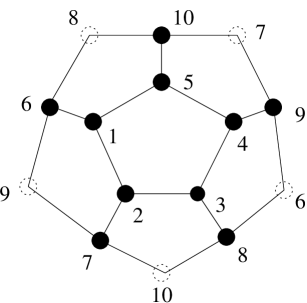
Figure 26: The convention for the numbering of the vertices of the dodecahedron in Appendix A. Points lying on the lower half–sphere are drawn as dotted circles. The projections of the points 1-5 to the lower half–sphere are not drawn, but all their links can be seen here.

Not all the point pairs are directly linked to each other, but all are at most two links apart. There are no ambiguities in applying the geodesic rule, because no pairs can be connected in more than one way, if we only allow connection lengths of up to two links. For any assignment of such a restricted selection of elements of $\R P^{2}$ to the vertices of a triangle, we can therefore identify uniquely whether the triangle is penetrated by a string or not. This is equivalent to the statement that we could use the same flux definition as before, because none of the projections to the upper half–sphere of vectors pointing to the vertices of the DH are at right angles to each other. This correspondence will make the proof easier, because we can just check whether a given shortest path between two points crosses the equator and assign it a value of $-1$ if it does, or $1$ otherwise. The product of all links will then indicate whether there is a string present in a triangle (if the product is negative) or not. Now let us take e.g. the assignments 2, 5, 8, and 9 for the respective vacuum fields on the vertices of a tetrahedron. Then the links have the following “equator–crossing indicators” assigned to them:

$$\begin{array}[]{c}(25)\rightarrow+1\\ (28)\rightarrow+1\\ (29)\rightarrow-1\\ (58)\rightarrow-1\\ (59)\rightarrow+1\\ (89)\rightarrow+1\\ \end{array}$$

Since the two links which have $-1$ assigned to them are disconnected, all triangles border exactly one of the two links, and all the link–variable products are negative. There are therefore four string segments entering the tetrahedron.  $\Box$

Appendix B Renormalization Groups

B.1 Vacuum Field Averaging

Let us group the eight points of the bcc lattice cells spanned by the vectors $(1,0,0)$, $(0,1,0)$, and $(\frac{1}{2},\frac{1}{2},\frac{1}{2})$ such that the most frequently occurring vacuum value will be the value assigned to the super–site. In case of ambiguities, i.e. if two values occur three times each or four times each, we take the smaller value. Let us define the respective probabilities for the vacuum field values as

$$p(0)=p\,\,\,\,\,,\,\,\,\,\,p(1)=p(2)=\frac{1-p}{2}\,\,\,\,\,.\,\,\,\,\,$$ (28)

The possible configurations yielding, for the super-site, a field value of zero, then have respective probabilities as listed in Table 10.

field values	number of	probability
(+permutations)	permutations
(0,0,0,0,0,0,0,0)	1	$p^{8}$
(0,0,0,0,0,0,0,a)	$8\cdot 2$	$p^{7}\left(\frac{1-p}{2}\right)$
(0,0,0,0,0,0,a,a)	$27\cdot 2$	$p^{6}\left(\frac{1-p}{2}\right)^{2}$
(0,0,0,0,0,0,1,2)	56	$p^{6}\left(\frac{1-p}{2}\right)^{2}$
(0,0,0,0,0,a,a,a)	$56\cdot 2$	$p^{5}\left(\frac{1-p}{2}\right)^{3}$
(0,0,0,0,0,a,a,b)	$168\cdot 2$	$p^{5}\left(\frac{1-p}{2}\right)^{3}$
(0,0,0,0,1,1,1,1)	70	$p^{4}\left(\frac{1-p}{2}\right)^{4}$
(0,0,0,0,a,a,a,b)	$280\cdot 2$	$p^{4}\left(\frac{1-p}{2}\right)^{4}$
(0,0,0,0,1,1,2,2)	420	$p^{4}\left(\frac{1-p}{2}\right)^{4}$
(0,0,0,1,1,1,2,2)	560	$p^{3}\left(\frac{1-p}{2}\right)^{5}$

Table 10: The configurations of the eight sites grouped together to a supersite, which yield a vacuum value of 0 for the super–site, together with their respective probabilities, according to Eq. (28). It is assumed that $a\neq b$ and neither is equal to 0.

This gives, for the probability of the renormalized super–site to have a zero vacuum field

$$\begin{array}[]{rcl}p^{\prime}&=&P(p)\\[8.53581pt] &=&p^{8}+8p^{7}(1-p)+28p^{6}(1-p)^{2}+56p^{5}(1-p)^{3}+\frac{525}{8}p^{4}(1-p)^{4}+\frac{35}{2}p^{3}(1-p)^{5}\\[8.53581pt] &=&\frac{105}{8}p^{8}-55p^{7}+\frac{315}{4}p^{6}-\frac{63}{2}p^{5}-\frac{175}{8}p^{4}+\frac{35}{2}p^{3}\,\,\,\,\,.\end{array}$$ (29)

The polynomial $P(p)-p$ is plotted in Fig. 27. The zeros of this plot correspond to fixed points. Fixed points outside

 

Figure 27: The renormalization polynomial $P(p)-p$ of Eq. (29).

the range $[0,1]$ have no interpretation in terms of probabilities. We see that the only physical fixed points are at 0, $\frac{1}{3}$, and 1. They are all expected, as discussed in section 6.2. What is not discussed there is that the stability of the fixed points is determined by the sign of $dp^{\prime}/dp=dP/dp$ at the fixed points. As expected again, the fixed points 0 and 1 are the only stable ones, so that this renormalization procedure would get rid of all infinite strings for any $p\neq\frac{1}{3}$, which is clearly different from our measurements. A renormalization procedure that merely performs field averages is therefore not sufficient to describe the Hagedorn transition in the initial conditions (but it may perhaps describe the disappearance of infinite strings in the subsequent dynamical evolution, as observed in ref. [39]).

We stress that we haven’t been able to find any non-trivial fixed points for various generalisations of Eq. 29. It is straightforward to write down the renormalisation polynomial for general groupings of $n$ sites to a supersite, by generalising the criteria leading to valid entries in Table 10

$$p^{\prime} = P^{(n)}(p)$$ (30)

$$= \sum_{\begin{array}[]{c}{\scriptscriptstyle l,k=0}\\[-5.69054pt] {\scriptscriptstyle n-l\geq 2k}\\[-5.69054pt] {\scriptscriptstyle n-k\geq 2l}\end{array}}^{l,k\leq n/2}\frac{n!}{l!\,k!\,(n-l-k)!}\,p^{n-l-k}\left(\frac{1-p}{2}\right)^{k+l}\left(1-\frac{1}{2}\delta_{n-k-l,l}-\frac{1}{2}\delta_{n-k-l,k}+\frac{1}{3}\delta_{n,3l}\delta_{l,k}\right),$$ (34)

which does not seem to have any physical fixed points other than the trivial ones found with the polynomial in Eq. 29. The Kronecker deltas just divide out factors of two or three, depending on whether the most frequent vacuum phases are more than one, as e.g. in the fourth to last and last row of Table 10. We have tried the same approach for a minimally discretised $\R P^{2}$ symmetry where it is in fact much easier to write down the renormalisation polynomial for the bias, but again, all the fixed points are the trivial ones, and the percolation threshold cannot be located in this way. For completeness, the easily derivable renormalisation polynomial, if $p(0)=p(1)=p(2)=p/3$ and $p(3)=p(4)=p(5)=(1-p)/3$, and if we group a number $n$ of sites to become a supersite of the renormalised lattice, becomes

$$p^{\prime}=\sum_{k=0}^{[n/2]}\left[\left(\begin{array}[]{c}n\\ k\end{array}\right)p^{n-k}(1-p)^{k}\right]-\frac{1}{2}\delta_{2[n/2],n}\left(\begin{array}[]{c}n\\ n/2\end{array}\right)p^{n/2}(1-p)^{n/2}\,\,\,\,\,.\,\,\,\,\,$$

The bracket $[n/2]$ denotes the largest integer not larger than $n/2$, such that the term containing the Kronecker-delta corrects for the double counting of symmetric terms if $n$ is even. Again, the only physical fixed points for all of these polynomials (with $n>2$) are the trivial ones at $p=0,\frac{1}{2},1$, and no percolation threshold can be identified in this way.

B.2 Renormalizing the Vachaspati Model with Conserved Flux

As the next obvious step, one could try a renormalization procedure which conserves string flux. Clearly, this is most easily done for ₂ strings, where the string flux can only be 0 or 1 (or better: “even” or “odd”). As seen in all the models for ₂ strings (i.e. the Vachaspati model, our calculations for $\R P^{2}$, and the calculations of Kibble for $SO(3)$ strings [30]), this is essentially done by identifying lattice links as having one of the two values $\pm 1$ assigned to them, and taking the product over a closed contour. The obvious approach is therefore to associate two consecutive links with a super–link, and assigning to it the product of the two link values. On any lattice (cubic or tetrahedral), this preserves the string flux in the sense that the string flux through a super–plaquette is zero (even) if the sum of the string lines penetrating the constituent plaquettes is even, and odd (one) otherwise. The procedure is outlined in Fig. 28

 

Figure 28: The renormalization procedure for a grouping such that the coarse–grained lattice spacing is twice the spacing on the original lattice. The assignments to the links inside the finer lattice is irrelevant to the total string flux. Changing any of the outer links of the fine lattice changes the string flux, and changes one of the links of the coarse–grained lattice, changing the string flux also in the renormalized description.

The third dimension does not have to be drawn, since the renormalization procedures for differently oriented links are independent from each other (the second dimension is only necessary to show how changes in the string flux survive the renormalization procedure). Let us define the probability of finding a link with value $+1$ by $p_{+}=p$, such that $p_{-}=1-p$. Naively, one expects that, as the size of the super–plaquettes increases with every renormalization step, the string flux for very large plaquettes is 0 or 1 with equal probability, irrespective of the initial bias, as long as the average number of expected (non–renormalized) $(-1)$–links on the edge of the super–plaquette is $\gg 1$, i.e. for any non–trivial bias. The probabilities to have $-1$ or $+1$ assigned to a link converge towards $p_{-}=p_{+}=\frac{1}{2}$, i.e. $p_{+}=\frac{1}{2}$ should be a stable fixed point. This is exactly what happens: $p^{\prime}$ consists of two contributions: both links of the non–renormalized lattice have to have the same value assigned to them in order to make the super–link carry the value $+1$. Therefore

$$p^{\prime}=p^{2}+(1-p)^{2}\,\,\,\,\,.\,\,\,\,\,$$

It is easy to see that the only fixed points are $\frac{1}{2}$ and $1$. Furthermore, $dp^{\prime}/dp=4p-2$, such that $p=1$ is an unstable fixed point. $p=\frac{1}{2}$ is a stable fixed point and is approached exponentially fast for any sequence of renormalization steps.

This procedure cannot be refined by combining more than two links to a super–link in the next step, since the arguments leading to the very stable fixed point $p=\frac{1}{2}$ stay valid for any such renormalization. This has been tested up to coarse–grainings by factors of seven. The renormalization polynomial in any of these coarse–graining procedures is (if the lattice is coarse–grained by a factor of $N$)

$$p^{\prime}=P_{N}(p)=\sum_{k=0}^{k\leq N/2}\left(\begin{array}[]{c}N\\ (N{\rm mod}\,2)+2k\\ \end{array}\right)\,p^{N-2k}\,(1-p)^{2k}\,\,\,\,\,.\,\,\,\,\,$$

For which it is trivially true that $p=1$ and $p=\frac{1}{2}$ is a fixed point. Using

$$1+\left(\begin{array}[]{c}n\\ 2\\ \end{array}\right)+\left(\begin{array}[]{c}n\\ 4\\ \end{array}\right)+\ldots=2^{n-1}\,\,\,\,\,,\,\,\,\,\,\left(\begin{array}[]{c}n\\ 1\\ \end{array}\right)+\left(\begin{array}[]{c}n\\ 3\\ \end{array}\right)+\left(\begin{array}[]{c}n\\ 5\\ \end{array}\right)+\ldots=2^{n-1}\,\,\,\,\,,\,\,\,\,\,$$

it is easy to see that $p=\frac{1}{2}$ is also a fixed point for all of these renormalization procedures. Also, for odd numbers of $N$, $p=0$ is a fixed point, as one expects (an odd number of $(-1)$–links gets renormalized to a $(-1)$–super–link). we have tested $P_{N}(p)$ for values up to $N=7$, and the mentioned fixed points are really the only solutions of $P_{N}(p)=p$ for all of these. Furthermore, the speed of divergence of $P_{N}(p)$ outside the interval $[0,1]$ tends to increase, so that it seems that the physical fixed points are in fact the only real ones, and all other solutions to $P_{N}(p)=p$ are complex numbers. Surely it should be possible to find a rigorous proof for this statement, from the general form of $P_{N}(p)$, but instead we refer to Fig. 29, which seems to suggest very strongly a tendency for the $P_{N}(p)$ not to develop any other physical fixed points as we increase $N$.

 
 

Figure 29: The renormalization polynomial for orders 2 to 7. There is a clear tendency for the potential to flatten out near $p=\frac{1}{2}$, making the speed of convergence towards the stable fixed point $p=\frac{1}{2}$ faster for larger $N$. There is no tendency for the emergence of any fixed points other than 0 (for odd polynomials only), $\frac{1}{2}$, and 1. The dotted line is the line $p=p$. The intersections define the fixed points.

What this means is that the here proposed renormalization procedure is also inappropriate for telling us about the scaling of the string network, as all it tells us is that through very large surfaces (on super–horizon scales), the probability of finding a ₂–string flux 1 is $\frac{1}{2}$. In particular, it does not enable us to locate a string percolation threshold.

Summarising both sections of this appendix, the question of how to formulate a renormalization group transformation which identifies the Hagedorn transition point as a fixed point remains unanswered, as does the question of which variables one should preserve in such a transformation.

Appendix C Comparison to Thermal Quantities

In ref. [4] we attempted to extract a statistical temperature definition from the probability distribution of strings. This can of course only be done by analogy to statistical mechanics arguments. It will turn out that the thus obtained temperature is meaningless in physical terms, and that we arrive at a circular argument, giving us that $c$ should be interpreted as an inverse temperature, which is not the case, as we argued before. Thus, comparisons with thermal ensembles or thermal partition functions are not appropriate.

If we define a probability density that a given string segment belongs to a loop in the length interval $[l,l+dl]$ by $P(l)\propto(l\,{dn}/{dl})$, we can define an information entropy, contained in the probability distribution function by

$$S=-\sum_{l}P(l)\ln P(l)\,\,\,\,\,.\,\,\,\,\,$$

We can for instance try to relate the average length of string loops to an average energy of a thermal ensemble. It would then make sense to define a temperature $\theta$ as

$$\frac{1}{\theta}=\frac{\partial S}{\partial\langle l\rangle}\,\,\,\,\,,\,\,\,\,\,$$

and see how the system behaves under changes of the bias. In ref. [4] we did not have good enough statistics to extract that parameter, but with the partition function we do not need to get involved with the numerically highly unstable division of two differentials, because, without normalization,

$$P(l)=l^{-\tau+1}e^{-cl}\,\,\,\,\,.\,\,\,\,\,$$

The entropy can then be split into two parts

$$S=-\sum_{l}l^{-\tau+1}e^{-cl}\left[(-\tau+1){\rm ln}\,l-cl\right]=S_{1}+S_{2}\,\,\,\,\,.\,\,\,\,\,$$

Then

$$S_{2}\propto c\langle l_{\rm loop}\rangle\propto c^{\tau-2}\,\,\,\,\,.\,\,\,\,\,$$

$S_{1}$, by partial integration, behaves as

$$\begin{array}[]{rcl}S_{1}&\propto&\int{\rm ln}\,(l)\,l^{-\tau+1}e^{-cl}\,dl\\ &\propto&c^{\tau-2}\left[{\rm const}_{1}-{\rm const}_{2}\,{\rm ln}c\right]\,\,\,\,\,,\end{array}$$

Thus, with

$$dS\propto(\Delta\eta)^{\frac{\tau-2-\sigma}{\sigma}}[1+{\rm const}\,{\rm ln}\eta]d(\Delta\eta)\,\,\,\,\,,\,\,\,\,\,$$

and

$$d\langle l_{\rm loop}\rangle\propto(\Delta\eta)^{\frac{\tau-3-\sigma}{\sigma}}d(\Delta\eta)\,\,\,\,\,,\,\,\,\,\,$$

we obtain

$$\theta\propto(\Delta\eta)^{-\frac{1}{\sigma}}[1+{\rm const}\,{\rm ln}\eta]\,\,\,\,\,,\,\,\,\,\,$$

and the thus obtained temperature diverges, up to logarithmic corrections, as $1/c$, and the Hagedorn transition happens at infinite $\theta$. Thus, the correspondence of our partition function with a thermal one does not hold.   $\Box$

References

- [1] Ya.B. Zel’dovich, I.Yu. Kobzarev and L.B. Okun, Sov. Phys. JETP 40 (1975) 1 (Zh. Eksp. Teor. Fiz. 67 (1974) 3).
- [2] D. Coulson, Z. Lalak and B. Ovrut, Phys. Rev. D53 (1996) 4237.
- [3] T. Vachaspati, Phys. Rev. D44 (1991) 3723.
- [4] M. Hindmarsh and K. Strobl, Nucl. Phys. B437 (1995) 471.
- [5] P.G. de Gennes, Scaling Concepts in Polymer Physics, (Cornell University Press, Ithaca, 1979).
- [6] T.W.B. Kibble, J. Phys. A 9 (1976) 1387.
- [7] A. Vilenkin and E.P.S. Shellard, Cosmic Strings and other Topological Defects (Cambridge Univ. Press, Cambridge,1994).
- [8] M.B. Hindmarsh and T.W.B. Kibble, Rep. Prog. Phys. 58 (1995) 477.
- [9] P. Ferreira and N. Turok, unpublished.
-
[10]
K. Strobl, Aspects of Approximate Symmetry in
Cosmology and Nematic Liquid Crystals (PhD thesis, Cambridge
University, 1995)
(http://starsky.pcss.maps.susx.ac.uk/users/karls/thesis/index.html). - [11] J. Borrill, Phys. Rev. Lett. 76 (1996) 3255.
- [12] Imperial College preprint IMPERIAL-TP-95-96-27 (astro-ph/9602131).
- [13] K. Strobl, in preparation.
- [14] Y.B. Zel’dovich, I.Y. Kobzarev and L.B. Okun, Phys. Lett. 50B (1974) 340.
- [15] P.H. Frampton and T.W. Kephart, Phys. Rev. D51 (1995) 1.
- [16] R. Leese and T. Prokopec, Phys. Lett. B260 (1991) 27.
- [17] K. Strobl, Sussex University preprint SUSX-TH-96-012 (hep-lat/9608085).
- [18] T. Vachaspati and A. Vilenkin, Phys. Rev. D30 (1984) 2036.
- [19] S. Rudaz and A.M. Srivastava, Mod. Phys. Lett. A8 (1993) 1443.
- [20] M. Hindmarsh, A-C. Davis and R. Brandenberger Phys. Rev. D49 (1994) 1944.
- [21] E. Copeland, D. Haws, T.W.B. Kibble, D. Mitchell and N. Turok, Nucl. Phys. B298 (1988) 445.
- [22] R.A. Leese and T. Prokopec, Phys. Rev. D44 (1991) 3749.
- [23] B. Li, N. Madras and A.D. Sokal, New York Univ. preprint NYU–TH–94–09–01 (Sep. 1994) (hep-lat/9409003).
- [24] K. Strobl, in preparation.
- [25] A.D. Sokal, in Monte Carlo and Molecular Dynamics Simulations in Polymer Science, Kurt Binder ed. (Oxford University Press, Oxford, 1994).
- [26] R.J. Scherrer and J.A. Frieman, Phys. Rev. D33 (1986) 3556.
- [27] A. Vilenkin, in The Very Early Universe, G. Gibbons, S.W. Hawking and S.T.C. Siklos eds.
- [28] R.M. Bradley, P.N. Strensky, and J.-M. Debierre, Phys. Rev. A45 (1992) 8513.
-
[29]
I. Chuang, R. Dürrer, N. Turok and B. Yurke,
Science 251 (1991) 1336;
I. Chuang, B. Yurke, A.N. Pargelis and N. Turok, Phys. Rev. E47 (1993) 3343. - [30] T.W.B. Kibble, Phys. Lett. 166 B (1986) 311.
- [31] R. Hagedorn, Nuovo Cim. Supp. 3 (1965) 147.
- [32] M.J. Bowick and L.C.R. Wijewardhana, Phys. Rev. Lett. 54 (1985) 2485.
- [33] D. Mitchell and N. Turok, Nucl. Phys. B294 (1987) 1138.
-
[34]
E. Copeland, D. Haws and R. Rivers, Nucl. Phys. B319 (1989) 687;
E. Copeland, D. Haws, S. Holbraad and R. Rivers, Physica A 179 (1991) 507. - [35] D. Stauffer and A. Aharony, Introduction to Percolation Theory (Taylor & Francis, London, 1991).
- [36] E. Copeland, D. Haws, S. Holbraad and R. Rivers, Phys. Lett. B236 (1990) 49.
- [37] H. Georgi, S. Glashow and M. Wise, Phys. Rev. Lett. 47 (1981) 402.
-
[38]
M. Kamionkowski and J. March–Russell, Phys. Lett. 282B (1992) 137;
R. Holman et al., Phys. Lett. 282B (1992) 132. - [39] M. Mondello and N. Goldenfeld, Phys. Rev. A45 (1992) 657.