DFTT 31/96

IFUM 535/96 FT

NORDITA 43/96 P

SISSA 101/96/EP

hep-th/9607032

July, 1996

Spontaneous $N=2\,\rightarrow\,N=1$
local supersymmetry breaking
with surviving compact gauge groups^∗
Pietro Fré ¹, Luciano Girardello ², Igor Pesando¹ and Mario Trigiante³

¹ Dipartimento di Fisica Teorica, Universitá di Torino, via P. Giuria 1, I-10125 Torino,
Istituto Nazionale di Fisica Nucleare (INFN) - Sezione di Torino, Italy
and Nordita, Blegdamsvej 17, DK-1200 Copenhagen  OE, Denmark
² Dipartimento di Fisica, Università di Milano, via Celoria 6, I-20133 Milano,
and Istituto Nazionale di Fisica Nucleare (INFN) - Sezione di Milano, Italy
³ International School for Advanced Studies (ISAS), via Beirut 2-4, I-34100 Trieste
and Istituto Nazionale di Fisica Nucleare (INFN) - Sezione di Trieste, Italy

Abstract

Generic partial supersymmetry breaking of $N=2$ supergravity with zero vacuum energy and with surviving unbroken arbitrary gauge groups is exhibited. Specific examples are given.  ^∗ Supported in part by EEC Science Program SC1*CT92-0789.

1 Introduction

$N=2$ supergravity and $N=2$ rigid gauge theory have recently played a major role in the discussion of string–string dualities [1, 2, 3, 4, 5, 6, 7] and in the analysis of the non–perturbative phases of Yang–Mills theories [8, 9, 10, 11]. Furthermore in its ten years long history, $N=2$ supergravity has attracted the interest of theorists because of the beautiful and rich geometrical structure of its scalar sector, based on the manifold:

$${\cal M}_{scalar}={\cal SK}_{n}\,\otimes\,{\cal Q}_{m}$$ (1.1)

where ${\cal SK}_{n}$ denotes a complex $n$–dimensional special Kähler manifold [12, 13, 14, 15, 16] (for a review of Special Kähler geometry see either [17] or [18]) and ${\cal Q}_{m}$ a quaternionic $m$–dimensional quaternionic manifold, $n$ being the number of vector multiplets and $m$ the number of hypermultiplets [19, 20, 21, 15].

In spite of its beauty and of its significant role in understanding the structure of non perturbative field and string theory, applications of $N=2$ supergravity to the description of the real world have been hampered by the presence of mirror fermions and by a tight structure which limits severely the mechanisms of spontaneous breaking of local $N=2$ SUSY. Any attempt to investigate the fermion problem requires a thorough understanding of the spontaneous breaking with zero vacuum energy. In particular, an interesting feature is the sequential breaking to $N=1$ and then to $N=0$ at two different scales. Sometimes ago a negative result on partial breaking was established within the $N=2$ supergravity formulation based on conformal tensor calculus [22]. A particular way out was indicated in an ad hoc model [23] which prompted some generalizations based on Noether couplings [24].

With the developments in special Kähler geometry [25, 4, 5] stimulated by the studies on S–duality, the situation can now be cleared in general terms. Indeed it has appeared from [26, 27, 28, 29] that the negative results on $N=2$ partial supersymmetry breaking were the consequence of unnecessary restrictions imposed on the formulation of special Kähler geometry and could be removed.

In this paper we discuss in detail the generic structure of partial breaking within the general form of $N=2$ supergravity theory coupled to an arbitrary number of vector multiplets and hypermultiplets and with an arbitrary gauging of the scalar manifold isometries. In particular an explicit example is worked out in section 3, based on the choice for the vector multiplets of the special Kähler manifold $SU(1,1)/U(1)\,\otimes\,SO(2,n)/SO(2)\times SO(n)$ and of the quaternionic manifold $SO(4,m)/SO(4)\times SO(m)$ for the hypermultiplets.

1.1 The bearing of the coordinate free definition of Special Kähler geometry

A main point in our subsequent discussion is the use of symplectic covariance within the coordinate free definition of special Kähler geometry [14, 15].

Adopting the conventions of [30] a complex $n$–dimensional Hodge–Kähler manifold is special Kähler of the local type if there exists a bundle ${\cal H}={\cal SV}\otimes{\cal L}$ where ${\cal SV}\stackrel{{\scriptstyle\pi}}{{\longrightarrow}}{\cal M}_{n}$ is a holomorphic flat vector bundle of rank $2n+2$ with structural group $Sp(2n+2,{\rm I\kern-1.79993ptR})$, while ${\cal L}\stackrel{{\scriptstyle\pi}}{{\longrightarrow}}{\cal M}_{n}$ is the line bundle whose first Chern class equals the Kähler class ($K=c_{1}({\cal L}$) and if there exists a symplectic section of ${\cal H}$, named $\Omega$ such that:

$$K={{\rm i}\over{2\pi}}\,\partial\,{\overline{\partial}}\,{\rm lg}\,\left({\rm i}\langle\Omega|{\overline{\Omega}}\rangle\right)\,\equiv\,{{\rm i}\over{2\pi}}\,\partial\,{\overline{\partial}}\,{\rm lg}\,\left({\rm i}\Omega^{T}\,\left(\matrix{{\bf 0}&{\bf 1}\cr-{\bf 1}&{\bf 0}\cr}\right){\overline{\Omega}}\right)$$ (1.2)

the boldfaced blocks in the above equation being $(n+1)\times(n+1)$ matrices. Naming $\{z^{i}\}$ a set of coordinates for ${\cal M}_{n}$, the symplectic section $\Omega$ is usually written as:

$$\Omega=\left(\matrix{X^{\Lambda}(z)\cr F_{\Sigma}(z)}\right)$$ (1.3)

where the capital Greek indices run on $n+1$ values and label the full set of vector fields of the theory including the graviphoton ($\Lambda=0$). The upper half of the symplectic section is therefore associated with the electric gauge potentials and it could be defined as the coefficient of the gravitino contribution to the supersymmetry variation of these fields:

$$\delta_{SUSY}A^{\Lambda}_{\mu}=\dots+{\rm const}\,e^{{\cal K}}\,X^{\Lambda}(z)\,{\overline{\epsilon}}^{A}\,\psi_{\mu}^{B}\,\varepsilon_{AB}\,+\dots$$ (1.4)

where $e^{{\cal K}}$ denotes the exponential of the Kähler potential. The lower part of the symplectic section $F_{\Sigma}(z)$, which enters the construction of the supersymmetric lagrangian in several ways, would play, in the supersymmetry transformation rule of the dual magnetic potentials $A_{\Sigma|\mu}^{(magn.)}$, had we introduced them, the same role as it is played by $X^{\Lambda}(z)$ in the transformation rule of the electric potentials.

A built in feature of special geometry is the possibility of performing symplectic transformations of $Sp(2n+2,{\rm I\kern-1.79993ptR})$. Such transformations correspond to changes of bases for the symplectic sections in the bundle ${\cal H}$. Under such transformations the notion of electric and magnetic gauge fields changes and in fact the $Sp(2n+2,{\rm I\kern-1.79993ptR})$ are realized as duality transformations which are never symmetries of the lagrangian but they can be symmetries of the field equations plus Bianchi identities when they correspond to the symplectic embedding of isometries of the scalar manifold. If the symplectic transformations are not symmetries, they are anyhow conceivable field redefinitions and the question is whether they yield equivalent formulations of the same theory. The answer is that such physical equivalence occurs only in the case of ungauged theories, namely when all the electric charges are set to zero and the gauge group is abelian. Indeed it is only in this case that distinction between electric and magnetic fields is immaterial. As soon as an electric current is introduced the distinction is established and, at least at the classical (or semiclassical) level, the only symplectic transformations that yield equivalent theories (or can be symmetries) are the perturbative ones generated by lower triangular symplectic matrices:

$$\left(\matrix{{\bf A}&{\bf 0}\cr{\bf C}&{\bf D}\cr}\right)\,$$ (1.5)

It follows that different bases of symplectic sections for the bundle ${\cal H}$ yield, after gauging, inequivalent physical theories. The possibility of realizing or not realizing partial supersymmetry breaking $N=2\,\rightarrow\,N=1$ are related to this choice of symplectic bases. In the tensor calculus formulation the lower part of the symplectic section $F_{\Lambda}(z)$ should be, necessarily, derivable from a holomorphic prepotential $F(X)$ that is a degree two homogeneous function of the upper half of the section:

$$F_{\Sigma}(z)={{\partial}\over{\partial X^{\Sigma}(z)}}\,F(X(z))\quad;\quad F\left(\lambda\,X^{\Sigma}(z)\,\right)=\,\lambda^{2}\,F\left(X^{\Sigma}(z)\,\right)$$ (1.6)

This additional request is optional in the more general geometric formulation of $N=2$ supergravity [15, 30] where only the intrinsic definition of special geometry is utilized for the construction of the lagrangian. It can be shown that the condition for the existence of the holomorphic prepotential $F(X)$ is the non degeneracy of the jacobian matrix $e^{I}_{i}(z)\equiv\partial_{i}\left(X^{I}/X^{0}\right);I=1,\dots,n$. There are symplectic bases where this jacobian has vanishing determinant and there no $F(X)$ can be found. If one insists on the existence of the prepotential such bases are discarded a priori.

There is however another criterion to select symplectic bases which has a much more intrinsic meaning and should guide our choice. Given the isometry group $G$ of the special Kähler manifold ${\cal SV}$, which is an intrinsic information, which subgroup of $G_{class}\subset G$ is realized by classical symplectic matrices $\left(\matrix{{\bf A}&{\bf 0}\cr{\bf 0}&{\bf D}\cr}\right)$ and which part of $G$ is realized by non perturbative symplectic matrices $\left(\matrix{{\bf A}&{\bf B}\cr{\bf C}&{\bf D}\cr}\right)$ with ${\bf B}\neq 0$ is a symplectic base dependent fact. It appears that in certain cases, very relevant for the analysis of string inspired supergravity, the maximization of $G_{class}$, required by a priori symmetry considerations, is incompatible with the condition ${\rm det}\left(e^{I}_{i}(z)\right)\,\neq\,0$ and hence with the existence of a prepotential $F(X)$. If the unneccessary condition on $F(X)$ existence is removed and the maximally symmetric symplectic bases are accepted the no-go results on partial supersymmetry breaking can also be removed. Indeed in [26] it was shown that by gauging a group

$$G_{gauge}={\rm I\kern-1.79993ptR}^{2}$$ (1.7)

in a N=2 supergravity model with just one vector multiplet and one hypermultiplet based on the scalar manifold:

$${\cal SK}={{SU(1,1)}\over{U(1)}}\quad\quad;\quad\quad{\cal Q}={{SO(4,1)}\over{SO(4)}}$$ (1.8)

supersymmetry can be spontaneously broken from $N=2$ down to $N=1$, provided one uses the symplectic basis where the embedding of $SU(1,1)\equiv SL(2,{\rm I\kern-1.79993ptR})$ in $Sp(4,{\rm I\kern-1.79993ptR})$ is the following :

$$\forall\,\left(\matrix{a&b\cr c&d\cr}\right)\,\in\,SL(2,{\rm I\kern-1.79993ptR})\quad{\stackrel{{\scriptstyle\iota_{\delta}}}{{\hookrightarrow}}}\left(\matrix{a\,{\rm 1\kern-3.50006pt1}&b\,\eta\cr c\,\eta&d\,{\rm 1\kern-3.50006pt1}\cr}\right)\,\in\,Sp(4,{\rm I\kern-1.79993ptR})$$ (1.9)

1.2 Our results

In the present paper we generalize the above result to the case of an N=2 supergravity with $n+1$ vector multiplets and $m$ hypermultiplets based on the scalar manifold:

$${\cal SK}_{n+1}={{SU(1,1)}\over{U(1)}}\otimes{{SO(2,n)}\over{SO(2)\otimes SO(n)}}\quad\quad;\quad\quad{\cal Q}_{m}={{SO(4,m)}\over{SO(4)\otimes SO(m)}}$$ (1.10)

We show that we can obtain partial breaking $N=2\,\rightarrow\,N=1$ by

• choosing the Calabi–Vesentini symplectic basis where the embedding of $SL(2,{\rm I\kern-1.79993ptR})\otimes SO(2,n)$ into $Sp(4+2n,{\rm I\kern-1.79993ptR})$ is the following:

  $$\forall\,\left(\matrix{a&b\cr c&d\cr}\right)\,\in\,SL(2,{\rm I\kern-1.79993ptR}) {\stackrel{{\scriptstyle\iota_{\delta}}}{{\hookrightarrow}}} \left(\matrix{a\,{\rm 1\kern-3.50006pt1}&b\,\eta\cr c\,\eta&d\,{\rm 1\kern-3.50006pt1}\cr}\right)\,\in\,Sp(2n+4,{\rm I\kern-1.79993ptR})$$

  $$\forall\,L\,\in\,SO(2,n) {\stackrel{{\scriptstyle\iota_{\delta}}}{{\hookrightarrow}}} \left(\matrix{L&{\bf 0}\cr{\bf 0}&(L^{T})^{-1}\cr}\right)\,\in\,Sp(2n+4,{\rm I\kern-1.79993ptR})$$ (1.11)

  namely where all transformations of the group $SO(2,n)$ are linearly realized on electric fields

• gauging a group:

  $$G_{gauge}={\rm I\kern-1.79993ptR}^{2}\,\otimes\,G_{compact}$$ (1.12)

  where

  $${\rm I\kern-1.79993ptR}^{2}\, \cap SL(2,R)\otimes SO(2,n)=0$$

  $${\rm I\kern-1.79993ptR}^{2} \subset \mbox{ an abelian ideal of the solvable Lie subalgebra }V\,\subset so(4,m)$$

  $$G_{compact} \subset SO(n)\subset SO(2,n)$$

  $$G_{compact} \subset SO(m-1)\subset SO(4,m)$$ (1.13)

  namely where ${\rm I\kern-1.79993ptR}^{2}$ is a group of two abelian translations acting on the hypermultiplet manifold but with respect to which the vector multiplets have zero charge, while the compact gauge group $G_{compact}$ commutes with such translations and has a linear action on both the hypermultiplet and the vector multiplets.

The solvable Lie subalgebra $V\subset so(4,m)$ mentioned in eq. 1.13 is that subalgebra of the non–compact isometry group $G$ algebra such that, according to Alekseevski [31] (see also [32, 33, 34]), the quaternionic homogeneous manifold $G/H$ can also be identified with the group manifold ${\rm exp}[V]$.

In the following two sections we derive the result summarized above starting from the recently obtained complete form of N=2 supergravity with general scalar manifold interactions [30]. We conclude the present introduction with some physical arguments why the result should be obtained precisely in the way we have described.

1.3 General features of the partial $N=2$ supersymmetry breaking

To break supersymmetry from $N=2$ down to $N=1$ we must break the $O(2)$ symmetry that rotates one gravitino into the other. This symmetry is gauged by the graviphoton $A^{0}_{\mu}$. Hence the graviphoton must become massive. At the same time, since we demand that $N=1$ supersymmetry should be preserved, the second gravitino must become the top state of an $N=1$ massive spin $3/2$ multiplet which has the form $\left\{\left({{3}\over{2}}\right),{2}\left(1\right),\left({{1}\over{2}}\right)\right\}$. Consequently not only the graviphoton but also a second gauge boson $A^{1}_{\mu}$ must become massive through ordinary Higgs mechanism. This explains while the partial supersymmetry breaking involves the gauging of a two–parameter group. That it should be a non compact ${\rm I\kern-1.79993ptR}^{2}$ acting as a translation group on the quaternionic manifold is more difficult to explain a priori, yet we can see why it is very natural. In order to obtain a Higgs mechanism for the graviphoton $A_{\mu}^{0}$ and the second photon $A_{\mu}^{1}$ these vectors must couple to the hypermultiplets. Hence these two fields should gauge isometries of the quaternionic manifold ${\cal Q}$. This is obvious. That such isometries should be translations is understood by observing that in this way one introduces a flat direction in the scalar potential, corresponding to the vacuum expectation value of the hypermultiplet scalar, coupled to the vectors in such a way. Finally the need to use the correct symplectic basis is explained by the following remark. Inspection of the gravitino mass-matrix shows that it depends on both the momentum map ${\cal P}^{0}_{\Lambda}(q)$ for the quaternionic action of the gauge group on the hypermultiplet manifold and on the upper (electric) part of the symplectic section $X^{\Lambda}(z)$. In order to obtain a mass matrix with a zero eigenvalue we need a contribution from both $X^{0}$ and $X^{1}$ at the breaking point, which can always be chosen at $z^{i}=0$, since the vector multiplet scalars are neutral (this is a consequence of ${\rm I\kern-1.79993ptR}^{2}$ being abelian). Hence in the correct symplectic basis we should have both $X^{0}(0)\neq 0$ and $X^{1}(0)\neq 0$. This is precisely what happens in the Calabi–Vesentini basis for the special Kähler manifold $SU(1,1)/U(1)\otimes SO(2,n)/SO(2)\otimes SO(n)$. Naming $y^{i}$ $(i=1,\dots,n)$ a standard set of complex coordinates for the $SO(2,n)/(SO(2)\otimes SO(n))$ coset manifold, characterized by linear transformation properties under the $SO(2)\otimes SO(n)$ subgroup and naming $S$ the dilaton field, i.e. the complex coordinate spanning the coset manifold $SU(1,1)/U(1)$, the explicit form of the symplectic section (1.3) corresponding to the symplectic embedding (1.11) is (see [25] and [17]):

$$\Omega\,=\,\left(\matrix{X^{0}\cr X^{1}\cr X^{i}\cr F_{0}\cr F_{1}\cr F_{i}\cr}\right)\,=\,\left(\matrix{{{1}\over{2}}(1+y^{2})\cr\cr{\rm i}{{1}\over{2}}(1-y^{2})\cr\cr y^{i}\cr S\,{{1}\over{2}}(1+y^{2})\cr S\,{\rm i}{{1}\over{2}}(1-y^{2})\cr-\,S\,y^{i}\cr}\right)\,{\stackrel{{\scriptstyle y\,\rightarrow\,0}}{{\longrightarrow}}}\,\left(\matrix{{{1}\over{2}}\cr{\rm i}{{1}\over{2}}\cr 0\cr{{1}\over{2}}\,S\cr{\rm i}{{1}\over{2}}\,S\cr 0\cr}\right)$$ (1.14)

2 Formulation of the $N=2\rightarrow N=1$ SUSY breaking problem

As it is well understood in very general terms (see [35]), a classical vacuum of an $N=r$ supergravity theory preserving $p\leq r$ supersymmetries in Minkowski space–time is just a constant scalar field configuration $\phi^{I}(x)=\phi^{I}_{0}\,(I=1,\dots,\mbox{dim}\,{\cal M}_{scalar})$ corresponding to an extremum of the scalar potential and such that it admits $p$ Killing spinors. In this context, Killing spinors are covariantly constant spinor parameters of the supersymmetry transformation $\eta^{A}_{(a)}$ $(A=1,\dots,n)$, $(a=1,\dots,p)$ such that the SUSY variation of the fermion fields in the bosonic background $g_{\mu\nu}=\eta_{\mu\nu}\,,\,A^{\Lambda}_{\mu}=0\,,\,\phi^{I}=\phi^{I}_{0}$ is zero for each $\eta^{A}_{(a)}$:

$$\delta_{a}\,\psi_{\mu A} \equiv {\rm i}\gamma_{\mu}\,S_{AB}(\phi_{0})\,\eta^{B}_{(a)}\,=\,0$$

$$\delta_{a}\xi^{i} \equiv \Sigma^{i}_{A}(\phi_{0})\,\eta^{A}_{(a)}\,=\,0\quad\quad(a=1,\dots,p)$$ (2.1)

In eq.( 2.1) the spin ${{3}\over{2}}$ fermion shift $S_{AB}(\phi)$ and the spin ${{1}\over{2}}$ fermion shifts $\Sigma^{i}_{A}(\phi)$ are the non-derivative contributions to the supersymmetry transformation rules of the gravitino $\psi_{\mu A}$ and of the spin one half fields $\xi^{i}$, respectively. The integrability conditions of supersymmetry transformation rules are just the field equations. So it actually happens that the existence of Killing spinors, as defined by eq.( 2.1), forces the constant configuration $\phi^{I}=\phi^{I}_{0}$ to be an extremum of the scalar potential.

Hence we can just concentrate on the problem of solving eq.( 2.1) in the case $N=2$ with $p=1$.

In $N=2$ supergravity there are two kinds of spin one half fields: the gauginos $\lambda^{j^{\star}}_{A}$ carrying an $SU(2)$ index $A=1,2$ and a world–index $j^{\star}=1^{\star},\dots,n^{\star}$ of the tangent bundle $T^{(0,1)}{\cal SK}$ to the special Kähler manifold ($n=\mbox{dim}_{\bf C}\,{\cal SK}=\#\mbox{vector multiplets}$ ) and the hyperinos $\zeta^{\alpha}$ carrying an index $\alpha$=$(1,\dots,n)$ running in the fundamental representation of $Sp(2m,{\rm I\kern-1.79993ptR})$ ($m=\mbox{dim}_{\bf Q}\,{\cal Q}=\#\mbox{hypermultiplets}$ ). Hence there are three kind of fermion shifts:

$$\delta\psi_{\mu A} = i\gamma_{\mu}S_{AB}\eta^{B}$$

$$\delta(g_{i^{*}j}\lambda^{i^{*}}_{A}) = W_{j|AB}\eta^{B}$$

$$\delta\zeta^{\alpha} = N_{A}^{\alpha}\eta^{A}$$ (2.2)

According to the analysis and the conventions of [30, 15], the shifts are expressed in terms of the fundamental geometric structures defined over the special Kähler and quaternionic manifolds as follows:

$$S_{AB} = -{1\over 2}{\rm i}(\sigma_{x}\epsilon)_{AB}{\cal P}^{x}_{\Lambda}L^{\Lambda}$$

$$W_{j|AB} = -({\epsilon_{AB}}\partial_{j}{\cal P}_{\Lambda}L^{\Lambda}+{\rm i}(\sigma_{x}\epsilon)_{AB}{\cal P}^{x}_{\Lambda}f^{\Lambda}_{j})$$

$$N_{A}^{\alpha} = -2{\bf i}_{\vec{k}_{\Lambda}}{\cal U}^{\alpha}_{A}L^{\Lambda}\,=\,-2\,{\cal U}^{\alpha}_{A|u}\,k^{u}_{\Lambda}\,L^{\Lambda}$$ (2.3)

In eq.(2.3) the index $u$ runs on $4m$ values corresponding to any set of of $4m$ real coordinates for the quaternionic manifold. Further ${\cal P}_{\Lambda}$ is the holomorphic momentum map for the action of the gauge group ${\cal G}_{gauge}$ on the special Kähler manifold ${\cal SK}_{n}$, ${\cal P}^{x}_{\Lambda}\,(x=1,2,3)$ is the triholomorphic momentum map for the action of the same group on the quaternionic manifold, $L^{\Lambda}=e^{{\cal K}/2}X^{\Lambda}(z)$ is the upper part of the symplectic section (1.3), rescaled with the exponential of one half the Kähler potential ${\cal K}(z,{\overline{z}})$ (for more details on special geometry see [30], [17], [18]), ${\vec{k}}_{\Lambda}$ is the Killing vector generating the action of the gauge group on both scalar manifolds and finally ${\cal U}^{\alpha}_{A}$ is the vielbein 1–form on the quaternionic manifold carrying an $SU(2)$ doublet index and an index $\alpha$ running in the fundamental representation of $Sp(2m,{\rm I\kern-1.79993ptR})$.

In the case of effective supergravity theories that already take into account the perturbative and non–perturbative quantum corrections of string theory the manifolds ${\cal SK}$ and ${\cal Q}$ can be complicated non–homogeneous spaces without continuous isometries. It is not in such theories, however, that one performs the gauging of non abelian groups and that looks for a classical breaking of supersymmetry. Indeed, in order to gauge a non abelian group, the scalar manifold must admit that group as a group of isometries. Hence ${\cal M}_{scalar}$ is rather given by the homogeneous coset manifolds that emerge in the field theoretical limit to the tree level approximation of superstring theory. In a large variety of models the tree level approximation yields the choice ( 1.10) and we concentrate on such a case to show that a constant configuration with a single killing spinor can be found. Yet, as it will appear from our subsequent discussion, the key point of our construction resides in the existence of an ${\rm I\kern-1.79993ptR}^{2}$ translation isometry group on ${\cal Q}$ that can be gauged by two vectors associated with section components $X^{0}\,X^{1}$ that become constants in the vacuum configuration of ${\cal SK}$. That these requirements can be met is a consequence of the algebraic structure á la Alekseevski of both the special Kählerian and the quaternionic manifold. Since such algebraic structures exist for all homogeneous special and quaternionic manifolds, we are lead to conjecture that the partial supersymmetry breaking described below can be extended to most N=2 supergravity theories on homogenous scalar manifolds.

For the rest of the paper, however, we concentrate on the study of case (1.10).

In the Calabi-Vesentini basis (1.14) the origin $y=0$ of the vector multiplet manifold $SO(2,n)/SO(2)\otimes SO(n)$ is a convenient point where to look for a configuration breaking $N=2\,\rightarrow\,N=1$. We shall argue that for $y=0$ and for an arbitrary point in the quaternionic manifold $\forall q\,\in\,SO(4,m)/SO(4)\times SO(m)$ there is always a suitable group ${\rm I\kern-1.79993ptR}^{2}_{q}$ whose gauging achieves the partial supersymmetry breaking. Actually the group ${\rm I\kern-1.79993ptR}^{2}_{q}$ is just the conjugate, via an element of the isometry group $SO(4,m)$, of the group ${\rm I\kern-1.79993ptR}^{2}_{0}$ the achieves the breaking in the origin $q=0$. Hence we can reduce the whole analysis to a study of the neighborhood of the origin in both scalar manifolds. To show these facts we need to cast a closer look at the structure of the hypermultiplet manifold.

3 Explicit solution

3.1 The quaternionic manifold $SO(4,m)/SO(4)\otimes SO(m)$

We start with the usual parametrization of the coset $SO(4,m)\over SO(4)\otimes SO(m)$ [36]:

$${\rm I\kern-1.79993ptL}(q)=\left(\begin{array}[]{cc}\sqrt{1+qq^{t}}&q\\ q^{t}&\sqrt{1+q^{t}q}\end{array}\right)=\left(\begin{array}[]{cc}{r_{1}}&{q}\\ {q^{t}}&{r_{2}}\end{array}\right)$$ (3.1)

where $q=||q_{at}||$ is a $4\times m$ matrix . This coset manifold has a riemannian structure defined by the vielbein, connection and metric given below :

$${\rm I\kern-1.79993ptL}^{-1}d{\rm I\kern-1.79993ptL} = \left(\begin{array}[]{cc}\theta&E\\ E^{t}&\Delta\end{array}\right)\in so(4,m)$$ (3.4)

$$ds^{2} = E^{t}\otimes E$$ (3.5)

The explicit form of the vielbein and connections which we utilise in the sequel is:

$$E\,=\,r_{1}dq-qdr_{2}\quad;\quad\theta\,=\,r_{1}dr_{1}-qdq^{t}\quad;\quad\Delta\,=\,r_{2}dr_{2}-q^{t}dq$$ (3.6)

where $E$ is the coset vielbein, $\theta$ is the $so(4)$-connection and $\Delta$ is the $so(n)$-connection. The quaternionic structure of the manifold is given by

$$K^{x}\,=\,{1\over 2}tr(E^{t}\wedge J^{x}E)\quad;\quad\omega^{x}\,=\,-{1\over 2}tr(\theta J^{x})\quad;\quad{\cal U}^{A\alpha}\,=\,{1\over\sqrt{2}}E^{at}(e_{a})^{A}_{B}{}$$ (3.7)

$K^{x}$ being the triplet of hyperKähler 2–forms, $\omega^{x}$ the triplet of $su(2)$–connection 1–forms and ${\cal U}^{A\alpha}$ the vielbein 1–form in the symplectic notation. Furthermore $J^{x}$ is the triplet of $4\times 4$ self–dual ’t Hooft matrices $J^{+|x}$ normalized as in [30], $e_{a}$ are the quaternionic units as given in [30] and the symplectic index $\alpha=1,\dots,2m$ is identified with a pair of an $SU(2)$ doublet index $B=1,2$ times an $SO(4)$ vector index $t=1,\dots,m$: $\alpha\equiv Bt$. Notice also the factor ${1\over 2}$ in the definition of $K^{x}$ with respect to the conventions used in [30], which is necessary in order to have $\nabla\omega^{x}=-K^{x}$

3.2 Explicit action of the isometries on the coordinates and the killing vectors.

Next we compute the killing vectors; to this purpose we need to know the action of an element $g\in so(4,m)$ on the coordinates $q$. To this effect we make use of the standard formula

$$\delta{\rm I\kern-1.79993ptL}\equiv k^{at}_{g}\,{{\partial}\over{\partial q^{at}}}=g{\rm I\kern-1.79993ptL}-{\rm I\kern-1.79993ptL}w_{g}$$ (3.8)

where

$$w_{g}=\left(\begin{array}[]{cc}w_{1}&\\ &w_{2}\end{array}\right)\in so(4)\oplus so(m)$$ (3.9)

is the right compensator and the element $g\in so(4,m)$ is given by

$$g=\left(\begin{array}[]{cc}a&b\\ b^{t}&c\end{array}\right)\in{\bf so(4,m)}$$ (3.10)

with $a^{t}=-a$, $c^{t}=-c$. The solution to (3.8) is:

$$\delta q=aq+br_{2}-qc-q\widehat{w}_{2} = aq+r_{1}b-qc+\widehat{w}_{1}q$$

$$\delta r_{1}=[a,r_{1}]+bq^{t}-r_{1}\widehat{w}_{1} \delta r_{2}=[c,r_{2}]+b^{t}q-r_{2}\widehat{w}_{2}$$ ;

$$w_{1}=a+\widehat{w}_{1} w_{2}=c+\widehat{w}_{2}$$ ; (3.11)

The only information we need to know about $\widehat{w}_{1},\widehat{w}_{2}$ is that they depend linearly on $b,b^{t}$. Anyhow for completess we give their explicit form:

$$\widehat{w}_{1;ab} = \left.{d(\sqrt{{\hbox{ 1\kern-2.27621ptl}}+x})_{ab}\over dx_{cd}}\right|_{x=qq^{t}}(bq^{t}-qb^{t})_{cd}$$

$$\widehat{w}_{2;st} = \left.{d(\sqrt{{\hbox{ 1\kern-2.27621ptl}}+y})_{st}\over dy_{pq}}\right|_{y=q^{t}q}(b^{t}q-q^{t}b)_{pq}$$ (3.12)

¿From these expressions we can obtain the Killing vector field

$$\vec{k}_{g}=(\delta q)_{at}{\partial~{}\over\partial q_{at}}$$ (3.13)

3.3 The momentum map.

We are now in a position to compute the triholomorphic momentum map ${\cal P}^{x}_{g}$ associated with the generic element 3.10 of the $so(4,m)$ Lie algebra. Given the vector field 3.13, we are supposed to solve the first order linear differential equation:

$${\bf i}_{{\vec{k}}_{g}}K^{x}=-\nabla{\cal P}^{x}$$ (3.14)

$\nabla$ denoting the exterior derivative covariant with respect to the $su(2)$–connection $\omega^{x}$ and ${\bf i}_{{\vec{k}}_{g}}K^{x}$ being the contraction of the 2–form $K^{x}$ along the Killing vector field ${\vec{k}}_{g}$: By direct verification the general solution is given by:

$${\cal P}^{x}_{g}={1\over 2}tr(\left(\begin{array}[]{cc}{J^{x}}&{0}\\ {0}&{0}\end{array}\right)C_{g})=tr(J^{x}P_{g})$$ (3.15)

where for any element of the ${\bf so(4,m)}$ Lie algebra conjugated with the adjoint action of the coset representative (3.1), we have introduced the following block decomposition and notation:

$$\forall{g}\,\in\,{so(4,m)}:\quad C_{g}\,\equiv\,{\rm I\kern-1.79993ptL}(q)^{-1}g{\rm I\kern-1.79993ptL}(q)=\left(\begin{array}[]{cc}{2P_{g}}&{{\bf i}_{\vec{k}}E_{g}}\\ {{\bf i}_{\vec{k}}E^{t}_{g}}&{2Q_{g}}\end{array}\right)$$ (3.16)

Furthermore if we decompose $g=g^{\Lambda}\,{\bf T}_{\Lambda}$ the generic element $g$ along a basis $\{{\bf T}_{\Lambda}\}$ of generators of the $so(4,m)$ Lie algebra, we can write:

$${\cal P}^{x}_{\Lambda}={1\over 2}tr(\left(\begin{array}[]{cc}{J^{x}}&{0}\\ {0}&{0}\end{array}\right)C_{{\bf T}_{\Lambda}})=tr(J^{x}P_{{\bf T}_{\Lambda}})$$ (3.17)

3.4 Solution of the breaking problem in a generic point of the quaternionic manifold

At this stage we can attempt to find a solution for our problem i.e. introducing a gauging that yields a partial supersymmetry breaking.

Recalling the supersymmetry variations of the Fermi fields (2.2) we evaluate them at the origin of the special Kähler using the Calabi-Vesentini coordinates (1.14):

$$S_{AB}|_{y=0} = -{1\over 4}i(\sigma_{x}\epsilon)_{AB}tr(J^{x}(P_{0}+iP_{1}))$$

$$W_{s|AB}|_{y=0} = -{1\over 4(ImS)^{3\over 2}}i(\sigma_{x}\epsilon)_{AB}tr(J^{x}(P_{0}+iP_{1}))$$

$$W_{\alpha|AB}|_{y=0} = 0$$

$$N_{A}^{\alpha}|_{y=0} \propto ({\bf i}_{0}E^{at}-i{\bf i}_{1}E^{at}_{1})(e_{a})^{A}_{B}$$ (3.18)

where in the last equation we have identified $\alpha\equiv aB$ as explained after eq. ( 3.7 ).

In the next subsection we explicitly compute a solution for the matrices $P_{0},P_{1}$ and ${\bf i}_{0}E^{at},{\bf i}_{1}E^{at}$ at the origin of the quaternionic manifold ${\cal Q}_{m}$. Starting from this result it can be shown that any point $q\neq 0$ can define a vacuum of the theory in which SUSY is broken to $N=1$, provided a suitable gauging is performed. Indeed we can find the general solution for any point $q$ by requiring

$$C_{\Lambda}(q)=C_{\Lambda}(q=0)~{}~{}~{}~{}\Lambda=0,1$$ (3.19)

that is the group generators of the group we are gauging at a generic point $q$ are given by

$$T_{\Lambda}(q)={\rm I\kern-1.79993ptL}(q)T_{\Lambda}(0){\rm I\kern-1.79993ptL}^{-1}(q)$$ (3.20)

This result is very natural and just reflects the homogeneity of the coset manifold, i.e. all of its points are equivalent.

3.5 Solution of the problem at the origin of ${\cal Q}_{m}$.

In what follows all the earlier defined quantities, related to ${\cal Q}_{m}$, will be computed near the origin $q=0$. The right-hand side of equations (3.11,3.13) is expanded in powers of $q$ as it follows:

$$\delta q=b+aq-qc+O(q^{2}) \vec{k}_{a}\,=\,(aq)_{at}{\partial~{}\over\partial q_{at}}$$ ;

$$\vec{k}_{b}\,=\,b_{at}{\partial~{}\over\partial q_{at}} \vec{k}_{c}\,=\,-(qc)_{at}{\partial~{}\over\partial q_{at}}$$ ; (3.21)

The expressions for the vielbein, the connections and the quaternionic structure, to the approximation order we work, are:

$$E\,=\,dq-{1\over 2}qdq^{t}q \theta\,=\,{1\over 2}dqq^{t}-{1\over 2}qdq^{t}$$ ;

$$K^{x} = tr\left(dq^{t}~{}J^{x}~{}dq-dqq^{t}~{}J^{x}~{}dqq^{t}\right)$$

$$\omega^{x}\,=\,-{1\over 2}tr\left(dqq^{t}J^{x}\right) {\cal U}^{A\alpha}\,=\,{1\over\sqrt{2}}dq^{at}(e_{a})^{A}_{B}{}$$ ; (3.22)

Finally the triholomorphic momentum maps corresponding to the a,b,c generators, have the following form, respectively :

$${\cal P}^{x}_{a}\,=\,{1\over 2}tr(J^{x}a+J^{x}qt^{t}a)\quad;\quad{\cal P}^{x}_{b}\,=\,-{1\over 2}tr(J^{x}qb^{t})\quad;\quad{\cal P}^{x}_{c}\,=\,-{1\over 2}tr(J^{x}qcq^{t})$$ (3.23)

Inserting eq.s (3.23) into equations (3.18) one finds the expressions for the shift matrices in the origin:

$$S_{AB}|_{y=0} = -{1\over 4}i(\sigma_{x}\epsilon)_{AB}tr(J^{x}(a_{0}+ia_{1}))$$

$$W_{s|AB}|_{y=0} = -{1\over 4(ImS)^{3\over 2}}i(\sigma_{x}\epsilon)_{AB}tr(J^{x}(a_{0}+ia_{1}))$$

$$W_{\alpha|AB}|_{y=0} = 0$$

$$N_{A}^{\alpha}|_{y=0} \propto (b_{0}^{at}-ib^{at}_{1})(e_{a})^{A}_{B}{}$$ (3.24)

$a_{0,1}$ and $b_{0,1}$ being the a and b blocks of the matrices $P_{0,1}$, respectively.

It is now clear that in order to break supersymmetry we need $a\neq 0$ and $b\neq 0$ . From the first two equations and from the requirement that the gravitino mass–matrix $S_{AB}$ should have a zero eigenvalue we get

$$\sum_{x}(a_{0}+ia_{1})^{2}_{x}=0\Rightarrow\vec{a}_{0}\cdot\vec{a}_{1}=(\vec{a}_{0})^{2}-(\vec{a}_{1})^{2}=0$$ (3.25)

We solve this constraint by setting ($a_{x}=-{1\over 4}tr(J^{x}a)$ )

$$a_{0x}=g_{0}\delta_{x1}~{}~{}~{}~{}a_{1x}=g_{1}\delta_{x2}$$ (3.26)

with $g_{0}=g_{1}$. These number are the gauge coupling constants of the repeatedly mentioned gauge group ${\rm I\kern-1.79993ptR}^{2}$. Note that due to the orthogonality of the antiself–dual t’Hooft matrices ${\overline{J}}^{x}$ to the self–dual ones $J^{x}$, the general solution is not as in eq. 3.26, but it involves additional arbitrary combinations of ${\overline{J}}^{x}$, namely:

$$a_{0}\,=\,g_{0}J^{1}+\overline{a}_{0x}\overline{J}^{x}\quad;\quad a_{1}\,=\,g_{1}J^{2}+\overline{a}_{1x}\overline{J}^{x}$$ (3.27)

For the conventions see [30]. To solve the last of eq.s ( 3.18 ) we set

$$b_{0}=\left(\begin{array}[]{c}0\\ \vec{\beta}_{0}\\ 0\\ 0\end{array}\right)~{}~{}~{}~{}b_{1}=\left(\begin{array}[]{c}0\\ 0\\ \vec{\beta}_{1}\\ 0\end{array}\right)$$ (3.28)

where $\vec{\beta}_{0}$ and $\vec{\beta}_{1}$ are $m$–vectors of the in the fundamental representation of $SO(m)$.

Now the essential questions are:

1. Can one find two commuting matrices belonging to the ${\bf so(4,m)}$ Lie algebra and satisfying the previous constraints? These matrices are the generators of ${\rm I\kern-1.79993ptR}^{2}$.

2. If so, which is the maximal compact subalgebra ${\bf G}_{compact}\subset{\bf so(4,m)}$ commuting with them, namely the maximal compact subalgebra of the centralizer $Z({\rm I\kern-1.79993ptR}^{2})$? ${\bf G}_{compact}$ is the Lie algebra of the maximal compact gauge group that can survive unbroken after the partial supersymmetry breaking.

Let $a_{2},b_{2},c_{2}$ denote the blocks of the commutator $[g_{0},g_{1}]$. To answer the first question we begin to seek a solution with $c=0$, and it is easily checked that also their commutator have vanishing block $c_{3}$. Let us now look at the condition $a_{2}=0$, namely

$$a_{2}=[a_{0},a_{1}]+b_{0}b_{1}^{t}-b_{1}b_{0}^{t}=2g_{0}g_{1}J^{3}+2\epsilon^{xyz}\overline{a}_{0}^{x}\overline{a}_{1}^{y}\overline{J}^{z}+{1\over 2}\vec{\beta}_{0}\cdot\vec{\beta}_{1}(J^{3}+\overline{J}^{3})=0$$ (3.29)

This equation can be solved if we set

$$\overline{a}_{0}^{x}\,=\,\gamma g_{0}\delta_{x1}\quad;\quad\overline{a}_{1}^{x}\,=\,\gamma g_{1}\delta_{x2}\quad;\quad\vec{\beta}_{0}\cdot\vec{\beta}_{1}=-4g_{0}g_{1}{}$$ (3.30)

and if $\gamma^{2}=1\,\leftarrow\,\gamma=\pm 1$. Now we are left to solve the equation $b_{2}=a_{0}b_{1}-a_{1}b_{0}=0$, which implies

$$(\gamma-1)g_{0}\vec{b}_{1}=(\gamma-1)g_{1}\vec{b}_{0}{}$$ (3.31)

This equation is automatically fulfilled if $\gamma=1$ for any choice of the $\vec{b}_{i}$s, while it is not consistent with the last of equations (3.30) if $\gamma=-1$. Thus the only admissible value for $\gamma$ is $1$.

Choosing $\vec{\beta}_{0}=(\beta_{0},0\dots 0)$ we can immediately answer the second question: for the normalizer of the ${\rm I\kern-1.79993ptR}^{2}$ algebra we have $Z_{\bf so(4,m)}\left({\rm I\kern-1.79993ptR}^{2}\right)={\bf so(m-1)}$, so that of the $m$ hypermultiplets one is eaten by the superHiggs mechanism and the remaining $m-1$ can be assigned to any linear representation of a compact gauge group that can be as large as $SO(m-1)$.

4 The $N=2\rightarrow N=1$ breaking problem in Alekseevskiǐ’s formalism.

There are two main motivations for the choice of Alekseevskiǐ’s formalism [31],[32] while dealing with the partial breaking of $N=2$ supersymmetry:

• it provides a description of the quaternionic manifold as a group manifold on which the generators of the ${\rm I\kern-1.79993ptR}^{2}$ act as traslation operators on two (say $t_{0},t_{1}$) of the $4m$ scalar fields, parametrizing ${\cal Q}_{m}$;

• as it will be apparent in the sequel, the fields $t_{0},t_{1}$ define flat directions for the scalar potential. They can be identified with the hidden sector of the theory, for their coupling to the gauge fields $A_{\mu}^{0}$ and $A_{\mu}^{1}$ is what determines the partial supersymmetry breaking.

Thus Alekseevskiǐ’s description of quaternionic manifolds provides a conceptually very powerful tool to deal with the SUSY breaking problem, even in the case in which ${\cal Q}$ is not a symmetric homogeneous manifold [37]. In what follows a sketchy overview of Alekseevskiǐ’s formalism applied to the symmetric quaternionic manifold ${\cal Q}_{m}$ will be given, and in terms of the corresponding quaternionic algebra, an explicit realization of the generators of the gauge group will be found.

4.1 The Quaternionic Algebra and Partial SUSY Breaking.

The starting point of Alekseevskiǐ’s description of quaternionic manifolds is a theorem stating that every Riemannian manifold ${\cal M}$ with a transitive isometry group ${\cal G}$ generated by a solvable Lie Algebra G (named a normal manifold), can be expressed as a group manifold whose Lie Algebra $G^{\prime}$ is a suitable subalgebra of $G$: ${\cal M}=e^{G^{\prime}}$ Therefore there exists a one-to-one correspondence between normal Riemmanian manifolds and solvable Lie Algebras (endowed with an euclidean metric). The quaternionic manifolds ${\cal Q}_{m}$ we are dealing with are normal and therefore they can be obtained exponentiating a certain solvable subalgebra $V\subset{\bf so(4,m)}$, called quaternionic algebra. Alekseevskiǐ classified the quaternionic manifolds in terms of the corresponding quaternionic algebras. Every quaternionic algebra $V$ is characterized by a quaternionic structure which is an algebra of antisymmetric endomorphisms of $V$ generated by three operators $J_{1},J_{2},J_{3}$ fulfilling the standard algebra of quaternionic imaginary units: $J_{\alpha}\dot{J}_{\beta}=-\delta_{\alpha\beta}\,{\rm Id}+\varepsilon_{\alpha\beta\gamma}J_{\gamma}$. Moreover a single antisymmetric endomorphism $J$ of a vector space such that $J^{2}=-Id$ is usually called a complex structure. A Kählerian Algebra is defined as the solvable Lie algebra generating a normal Kählerian manifold, and it is characterized by a complex structure $J$. A common feature of the quaternionic algebras $V_{m}$ generating ${\cal Q}_{m}$ is that they have the form $V_{m}=U\oplus\widetilde{U}$ where:

$$U\,=\,F_{0}\oplus K_{m} K_{m}\,=\,F_{1}\oplus F_{2}\oplus F_{3}\oplus Z$$ ;

$$\widetilde{U}\,=\,J_{2}U J_{1}U\,=\,U$$ ; (4.32)

The subspaces $F_{i}\quad i=0,1,2,3$, endowed with the complex structure $J_{1}$ are 2-dimensional Kählerian algebras generated respectively by $\{h_{i},g_{i}\},\quad[h_{i},g_{i}]=g_{i}\quad i=0,1,2,3$. The space $Z$ and its image $\widetilde{Z}$ through $J_{2}$ in $\widetilde{U}$ are the only parts of the whole algebra whose dimension depends on $m=\#~{}of~{}hypermultiplets$, and thus it is natural to choose the fields parametrizing them in some representation of ${\cal G}_{compact}$, for, as it was shown earlier, ${\cal G}_{compact}\subset SO(m-1)$. At fixed $m$ the $Z$-sector can provide enough scalar fields as to fill a representation of the compact gauge group. On the other hand the fields of the hidden sector are to be chosen in the orthogonal complement with respect to $Z$ and $\widetilde{Z}$ and to be singlets with respect to ${\cal G}_{compact}$. Indeed, by definition the fields of the hidden sectorinteract only with $A_{\mu}^{0}$ and $A_{\mu}^{1}$
The relations characterizing a generic quaternionic algebra $V=U\oplus\widetilde{U}$ are:

$$[U,U]\subset U;\hskip 42.67912pt[U,\widetilde{U}]\subset\widetilde{U};\hskip 42.67912pt[\widetilde{U},\widetilde{U}]\subset\{g_{0}\}$$ (4.33)

Using Alekseevskiǐ’s notation, an orthonormal basis for U is provided by $\{h_{i},g_{i}\quad(i=0,1,2,3),z^{\pm}_{k}(k=1,...,m-4)\}$, while for $\widetilde{U}$ an orthonormal basis is given by $\{p_{i},q_{i}\quad(i=0,1,2,3),\widetilde{z}^{\pm}_{k}\quad(k=1,...,m-4)\}$. All these generators are uniquely defined by the algebraic structure of $V_{m}$ which was determined in Alekseevskiǐ’s work [31], and have a simple representation in terms of the canonical basis of the full isometry algebra ${\bf so(4,m)}$.

The next step is to determine within this formalism, the generators of the gauge group. As far as the ${\rm I\kern-1.79993ptR}^{2}$ factor is concerned we demand it to act by means of translations on the coordinates of the coset representative ${\rm I\kern-1.79993ptL}(q)$. To attain this purpose the generators of the translations $T_{0},T_{1}$ will be chosen within an abelian ideal ${\cal A}\subset V_{m}$ and the representative of ${\cal Q}_{m}$ will be defined in the following way:

$${\rm I\kern-1.79993ptL}(t,b)\,=\,e^{T(t)}e^{G(b)}\quad(t) = t^{0},t^{1}\quad;\quad(b)=b^{1},...,b^{4m-2}$$

$$T(t)\,=\,t^{\Lambda}T_{\Lambda}\quad\Lambda=0,1 G(t)\,=\,b^{a}G_{i}\quad a=1,...,4m-2$$ ;

$$V_{m} = T\oplus G$$ (4.34)

It is apparent from eq.(4.34) that the left action of a transformation generated by $T_{\Lambda}$ amounts to a translation of the coordinates $t^{0},t^{1}$. The latter will define flat directions for the scalar potential. As the scalar potential depends on the quaternionic coordinates only through ${\cal P}^{x}_{\alpha}$ and the corresponding killing vector, to prove the truth of the above statement it suffices to show that the momentum-map ${\cal P}^{x}_{\alpha}(t,b)$ on ${\cal Q}_{m}$ does not depend on the variables $t^{\Lambda}$. Indeed a general expression for ${\cal P}^{x}_{\alpha}$ associated to the generator $T_{\alpha}i$ of ${\bf so(4,m)}$ is given by equation (3.15):

$${\cal P}^{x}_{\alpha}(t,b)=\frac{1}{2}tr({\rm I\kern-1.79993ptL}^{-1}(t,b)T_{\alpha}{\rm I\kern-1.79993ptL}(t,b){\cal J}^{x})=\frac{1}{2}tr(e^{-G}e^{-T}T_{\alpha}e^{T}e^{G}{\cal J}^{x})$$ (4.35)

If $T_{\alpha}$ is a generator of the gauge group, then either it is in $T$ or it is in the compact subalgebra. In both cases it commutes with $T$ allowing the exponentials of $T(t)$ to cancel against each other. It is also straightforward to prove that the Killing vector components on ${\cal Q}_{m}$ do not depend on $t^{\Lambda}$.

A maximal abelian ideal ${\cal A}$ in $V_{m}$ can be shown to have dimension $m+2$. Choosing

$${\cal A}=\left\{e_{1},g_{3},p_{0},p_{3},q_{1},q_{2},\widetilde{z}_{+}^{k}\right\}\quad\quad(k=1,...,m-4)$$ (4.36)

one can show that possible candidates for the role of translation generators are either $T_{\Lambda}$ or $T^{\prime}_{\Lambda}$ defined below:

$$T_{0} = e_{1}+g_{3}=E_{\epsilon_{l-3}-\epsilon_{l-2}}+E_{\epsilon_{l-3}+\epsilon_{l-2}},\quad T_{1}=p_{0}-p_{3}=E_{\epsilon_{l-3}+\epsilon_{l-1}}+E_{\epsilon_{l-3}-\epsilon_{l-1}}$$

$$T^{\prime}_{0} = p_{0}-p_{3}=E_{\epsilon_{l-3}-\epsilon_{l-1}}+E_{\epsilon_{l-3}+\epsilon_{l-1}}\,,\,T^{\prime}_{1}=q_{1}+q_{2}=-(E_{\epsilon_{l-3}+\epsilon_{l}}+E_{\epsilon_{l-3}-\epsilon_{l}})$$ (4.37)

where $\epsilon_{k},\quad k=1,...,l=\mbox{rank}({\bf so(4,m)})$ is an orthonormal basis of ${\rm I\kern-1.79993ptR}^{l}$ and $\epsilon_{i}\pm\epsilon_{j}$ are roots of $so(4,m)$. In the previous section we found constraints on the form of the ${\rm I\kern-1.79993ptR}^{2}$ generators in order for partial SUSY breaking to occur on a vacuum defined at the origin of ${\cal Q}_{m}$. The matrices $T_{\Lambda}$ fulfill such requirements. On the other hand one can check that also $T^{\prime}_{\Lambda}$ are fit to the purpose, even if they do not have the form predicted in the previous section.Indeed they cause the gravitino and gaugino shifts to be proportional (on the chosen background) to $g_{0}\sigma_{2}+ig_{1}\sigma_{3}$ (and not to $g_{0}\sigma_{1}+ig_{1}\sigma_{2}$) which, for $g_{0}=g_{1}$, has also a vanishing eigenvalue.

Taking $T_{\Lambda}$ as generators of ${\rm I\kern-1.79993ptR}^{2}$, it follows from their matrix form that the largest compact subalgebra of ${\bf so(4,m)}$ suitable for generating ${\cal G}_{compact}$ is ${\bf so(m-1)}$.

In the previous section it was shown that this choice for the generators $T_{a}$ of ${\cal G}$, actually corresponds to an $N=1$ invariant vacuum defined by the conditions:

$$y^{i}=0\quad;\quad b^{a}=0$$ (4.38)

As it was also pointed out before, any point on ${\cal Q}_{m}$ described by $q=(t,b)$ can define a vacuum on which SUSY is partially broken, provided that a suitable choice for the isometry generators to be gauged is done, e.g.:

$$T_{\alpha}(t,b)={\rm I\kern-1.79993ptL}(t,b)T_{\alpha}{\rm I\kern-1.79993ptL}(t,b)^{-1}$$ (4.39)

To this extent all the points on the surface spanned by $t^{0},t^{1}$ and containing the origin, require the same kind of gauging (as it is apparent from equation (4.39), and this is another way of justifying the flatness of the scalar potential along these two directions.

The existence of a Killing spinor guarantees that on the corresponding constant scalar field configuration $N=2$ SUSY is broken to $N=1$, and the scalar potential vanishes. Furthermore, as explained in [35] and already recalled, the existence of at least one Killing spinor implies the stability of the background,namely that it is an extremum of the scalar potential. We have explicitly verified that the configuration $(y=0;b=0)$ are minima of the scalar potential by plotting its projection on planes, corresponding to different choices of pairs $(y,b)$ of coordinates which were let to vary while keeping all the others to zero. The behaviour of all these curves shows a minimum in the origin, where the potential vanishes, as expected. Two very typical representatives of the general behaviour of such plots are shown in figure 1 and 2.

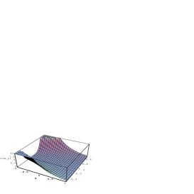
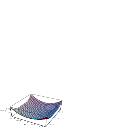
Figure 1: Scalar Potential Vs y generic and b coefficient of $e_{0}$

Figure 2: Scalar Potential Vs y generic and b coefficient of $h_{1}$.

5 Conclusion

It follows from our analysis that $N=2$ supergravity can be spontaneously broken to $N=1$ supergravity with the survival of unbroken rather arbitrary compact gauge groups. The fundamental catch in the derivation of the result is the use of the correct symplectic basis for special geometry and this is the one suggested by the symmetries of string theory. Here we have described $N=2$ partial breaking to $N=1$ by means of a classical superHiggs phenomenon in the context of a microscopic tree-level supergravity. It is conceivable that the further breaking of $N=1$ supersymmetry might proceed through a totally different mechanism, for instance gaugino condensation. In order to open new possibilities for phenomenological model building we still have to face the problem of vector like representations of the fermions. We have to look for a further mechanism to break the degeneracy between particles and their N=2 mirrors. It is also an interesting open question to find the relation of our mechanism with the non–perturbative $N=2$ supergravities predicted by string–string duality and with the conjectured non perturbative breaking caused by extremal black-holes [38].

References

- [1] S. Kachru and C. Vafa, Nucl. Phys. B450 (1995) 69, hep-th/9505105.
- [2] S. Ferrara, J. A. Harvey, A. Strominger and C. Vafa, Phys. Lett. B361 (1995) 59, hep-th/9505162.
- [3] M. Billó, R. D’Auria, S. Ferrara, P. Frè, P. Soriani and A. Van Proeyen, “R-symmetry and the topological twist of N=2 effective supergravities of heterotic strings”, preprint hep-th/9505123, to be published in Int. J. Mod. Phys. A.
- [4] M. Billó, A. Ceresole, R. D’Auria, S. Ferrara, P. Frè, T. Regge, P. Soriani and A. Van Proeyen, “A search for non–perturbative dualities of local N=2 Yang–Mills theories from Calabi–Yau three–folds”, preprint hep-th 9506075, to appear on Class and Quant. Grav.
- [5] I. Antoniadis, S. Ferrara, E. Gava, K.S. Narain and T.R. Taylor, Nucl. Phys. B447 (1995) 35, hep-th 9504034 (1995).
- [6] A. Sen ”Strong–Weak coupling duality in Four–dimensional String Theory” hep-th / 9402002.
- [7] A. Sen, Nucl. Phys B388 (1992) 457 and Phys. Lett. B303 (1993) 22; A Sen and J.H. Schwarz, Nucl. Phys. B411 (1994) 35; Phys. Lett. B312 (1993) 105.
- [8] N. Seiberg and E. Witten, Nucl. Phys. B426 (1994) 19.
- [9] N. Seiberg and E. Witten, Nucl. Phys. B431 (1994) 484.
- [10] A. Klemm, W. Lerche and P. Mayr, Phys. Lett. B357 (1995) 313, hep-th/9506112.
- [11] A. Klemm, W. Lerche and S. Theisen, “Nonperturbative Effective Actions of N=2 Supersymmetric Gauge Theories”, preprint CERN-TH/95-104, LMU-TPW 95-7, hep-th 9505150.
- [12] B. de Wit and A. Van Proeyen, Nucl. Phys. B245 (1984) 89;
- [13] B. de Wit, P. G. Lauwers and A. Van Proeyen Nucl. Phys. B255 (1985) 569.
- [14] L. Castellani, R. D’Auria and S. Ferrara, Phys. Lett. 241B (1990) 57,
- [15] R. D’Auria, S. Ferrara and P. Fré, Nucl. Phys. B359 (1991) 705.
- [16] A. Strominger, Comm. Math. Phys. 133 (1990) 163.
- [17] P. Fré, Nucl. Phys. B (Proc. Suppl.) 45B,C
- [18] A. Van Proeyen, KUL-TF-95-39, Dec 1995. 40pp. Lectures given at ICTP Summer School in High Energy Physics and Cosmology, Trieste, Italy, 12 Jun - 28 Jul 1995, hep-th/9512139
- [19] J. Bagger, E. Witten, Nucl. Phys. B 211 (1983) 302.
- [20] B. de Wit, R. Philippe, S.Q. Su and A. Van Proeyen Phys. Lett. B 134 (1984) 37.
- [21] K. Galicki, Comm. Math. Phys. 108 (1987) 117.
- [22] S. Cecotti, L. Girardello and M. Porrati, Phys. Lett. 145B (1984) 61.
- [23] S. Cecotti, L. Girardello and M. Porrati, Phys. Lett. 168 B (1986) 83.
- [24] Yu.M. Zinoviev Int. J. of Mod. Phys. A7 (1992) 7515, Yad. Fiz. 46 (1987) 943
-
[25]
A. Ceresole, R. D’Auria, S. Ferrara and A. Van Proeyen,
Nucl. Phys. B444 (1995) 92
“On Electromagnetic Duality in Locally Supersymmetric N=2 Yang–Mills Theory”, preprint CERN-TH.08/94, hep-th/9412200, Proceedings of the Workshop on Physics from the Planck Scale to Electromagnetic Scale, Warsaw 1994. - [26] S. Ferrara, L. Girardello and M. Porrati, Minimal Higgs Branch for the breaking of half of the Supersymmetries in N=2 Supergravity, Phys.Lett. B366 : p.155-159, 1996
- [27] I. Antoniadis, H. Partouche and T.R. Taylor, Spontaneous breaking of N=2 global supersymmetry, Phys.Lett. B372 :p.83-87, 1996
- [28] S. Ferrara, L. Girardello and M. Porrati, Spontaneous Breaking of N=2 to N=1 in Rigid and Local Supersymmetric Theories. hep-th/9512180, Phys. Lett. B376 (1996) 275
- [29] L. Alvarez Gaumé, J. Distler and C. Kounnas, Softly broken N=2 QCD, hep-th/9604004
- [30] L. Andrianopoli, M. Bertolini, A. Ceresole, R. D’Auria, S. Ferrara, P. Fré and T. Magri, hep-th/9605032, hep-th/9603004
- [31] D.V. Alekseevskii, Izv. Akad. Nauk. SSSR, Ser. Mat. Tom. 39 (1975) 297
- [32] S. Cecotti, Comm. Math. Phys. 124 (1989) 23
- [33] S. Cecotti, S. Ferrara and L. Girardello, IJMP A4 (1989) 2475
- [34] B. de Wit, F. Vanderseypen and A. Van Proeyen, Nucl. Phys. B400 (1993) 463
-
[35]
F. Cecotti, L. Girardello, M. Porrati: Proc. IX John Hopkins
Workshop, World Scientific 1985, Nucl. Phys. B 268 (1986) 265,
S. Ferrara and L. Maiani, Proc. V Silarg Symposium, World Scientific 1986,
For a general discussion see for instance the book
L. Castellani, R. D’Auria, P. Fré: “Supergravity and Superstring Theory: a geometric perspective”. World Scientific 1990, page 1078 and following ones (in particular eq. (IV.8.1)). - [36] See last item in the above reference, Vol I
-
[37]
V.A. Tsokur and Yu.M.Zinoviev, N=2 Supergravity models based on the nonsymmetric quaternionic manifolds.1.Symmetries and Lagrangian, hep-th/9605134,
V.A. Tsokur and Yu.M.Zinoviev, N=2 Supergravity models based on the nonsymmetric quaternionic manifolds.2.Gauge interactions, hep-th/9605143 - [38] R. Kallosh, Superpotential from balck holes, hep-th/9606093