FUB-HEP/95
Nonabelian Bosonization as a Nonholonomic Transformations from Flat to Curved Field Space.

Abstract

There exists a simple rule by which path integrals for the motion of a point particle in a flat space can be transformed correctly into those in curved space. This rule arose from well-established methods in the theory of plastic deformations, where crystals with defects are described mathematically by applying nonholonomic coordinate transformations to ideal crystals. In the context of time-sliced path integrals, this has given rise to a quantum equivalence principle which determines the measure of fluctating orbits in spaces with curvature and torsion. The nonholonomic transformations are accompanied by a nontrivial Jacobian which in curved spaces produces an additional energy proportional to the curvature scalar, thereby canceling an equal term found earlier by DeWitt from a naive formulation of Feynman’s time-sliced path integral in curved space. The importance of this cancelation has been documented in various systems (H-atom, particle on the surface of a sphere, spinning top). Here we point out its relevance in the process of bosonizing a nonabelian one-dimensional quantum field theory, whose fields live in a flat field space. Its bosonized version is a quantum-mechanical path integral of a point particle moving in a space with constant curvature. The additional term introduced by the Jacobian is crucial for the identity between original and bosonized theory.

A useful bozonization tool is the so-called Hubbard-Stratonovich formula for which we find a nonabelian version.

I Introduction

In 1956, Bryce DeWitt proposed a path integral formula in curved space using a specific generalization of Feynman’s time-sliced formula in cartesion coordinates [1]. Surprisingly, his amplitude turned out to satisfy a Schrödinger equation different from what had previously been considered as correct [2]: Apart from the Laplace-Beltrami operator for the kinetic term, he obtained an extra effective potential proportional to the scalar curvature $R$. At the time of his writing, DeWitt could not think of any argument to outrule the presence of such an extra term.

DeWitt’s work has had many successors [3]. These employed various time-slicings of the action, most popular being postpoint, midpoint, and prepoint prescriptions [4], and added to it different correction terms proportional to $\hbar^{2}$ to arrive at a Schrödinger equation of their personal preference.

In my opinion, such additional $\hbar^{2}$-terms must be rejected since they violate the basic principle of Feynman path integrals, according to which a quantum mechanical amplitude should be obtainable from a sum over all paths with an amplitude which is the exponential $e^{i{\cal A}_{\rm cl}/\hbar}$, where ${\cal A}_{\rm cl}$ is the purely classical action [5] along the path.

The apparent freedom in writing down various path integrals has its counterpart in the apparent freedom of setting up a time-evolution operator $\hat{H}$ from a classical action

$${\cal A}=\int dtL(q^{\mu}(t),\dot{q}^{\mu}(t))=\int dt\frac{M}{2}g_{\mu\nu}(q)\dot{q}^{\mu}\dot{q}^{\nu}$$ (1)

whose Hamiltonian contains products of momenta $p_{\mu}\equiv\partial L(q^{\mu}(t),\dot{q}^{\mu}(t))/\partial q^{\mu}$ and positions $q^{\mu}$:

$$H(p,q)=\frac{1}{2M}g^{\mu\nu}(q)p_{\mu}p_{\nu}.$$ (2)

The metric $g_{\mu\nu}(q)$ describes the geometry of configuration space. If the momenta $p_{\mu}$ are postulated to satisfy canonical commutation rules with the positions $q_{\nu}$, there are many different operator orderings corresponding to the same $H(p,q)$. This problem has become known as the operator-ordering problem, and its existence has caused a wide-spread myth among theoreticians, that it is basically unsolvable. In fact, many people have expressed their belief to the author that different physical systems might have to be quantized with different operator orderings.

Since some years, the author has been fighting this myth. There are many physical systems with a Hamiltonian of the form (2) for which we know a time-evolution operator $\hat{H}$ whose correctness has never been questioned. The most elementary example is the symmetric spinning top. If the classical Hamiltonian is written as in Eq. (2), with $q^{\mu}$ being the three Euler angles, and if $p_{\mu}$ abd $q^{\mu}$ are quantized canonically, there is of course an ordering problem. This, however, is due to having chosen the wrong classical variables for quantization. Since the system is invariant under rotations but not under translations, only the operators associated with the angular momenta $L_{i}$ have good quantum numbers, not the generators of translations $p_{\mu}$. One must therefore rewrite the classical Hamiltonian (2) as [6]

$$H=\frac{1}{2M}L_{i}^{2},$$ (3)

and impose commutation rules upon the angular momenta $L_{i}$:

$$[\hat{L}_{i},\hat{L}_{j}]=i\epsilon_{ijk}\hat{L}_{k}.$$ (4)

There is no operator-ordering problem in this procedure!

The same uniqueness holds for any Hamiltonian which is a linear combination of Casimir operators and generators of a group of motion in a curved configuration space. These observations form the basis of the so-called geometric quantization [7], in which there is no source for an extra $R$-term.

Thus we are faced with the problem of finding a construction procedure for path integrals in curved spaces which is naturally capable of reproducing these well-established results of group quantization. Since path integrals are formulated in phase space in terms of $p^{\mu}$ and $q^{\mu}$-variables which should not be used as a basis for quantization in the operator formulation, this seems to be a hard task. Nevertheless, a solution has been found in the form of a simple geometric mapping principle. The necessity for finding this solution came from the desire to solve the time-sliced path integral of the hydrogen atom, a task which was completed in a continumum formulation 17 years ago [8]. This solution proceeds by a three-step transformation to the path integral of a harmonic oscillator [9]. In the language of ordinary quantum mechanics, the three steps proceed as follows:
First, the Hamiltonian is extended by a dummy forth momentum $p_{4}$ and written as

$$H=\sum_{\mu=1}^{4}\frac{p_{\mu}^{2}}{2M}+\frac{e^{2}}{r},$$ (5)

Second, a nonholonomic Kustannheimo-Stiefel transformation to coordinates $u^{\mu}$ with $r=u^{2}=\sum_{\mu=1}^{4}{(u^{\mu})}^{2}$ is used to transform $H$ to

$$H=\sum_{\mu=1}^{4}\frac{p^{u}_{\mu}{}^{\,2}}{8Mu^{2}}+\frac{e^{2}}{u^{2}}.$$ (6)

This is of the form (2) and describes a system in a space with curvature. Only recently it was discovered that as a consequence of the nonholonomic nature of the transformation, the $u^{\mu}$-space carries also torsion [9, 10, 11].

Classical orbits satisfy energy conservation

$$H-E=0.$$ (7)

In a third step, the classical equation (8) is multiplied by $u^{2}$ and becomes

$$\sum_{\mu=1}^{4}\frac{p^{u}_{\mu}{}^{\,2}}{8M}+{e^{2}}-{u^{2}}E=0.$$ (8)

This has a unique operator version describing a harmonic oscillator.

The intermediate Hamiltonian (6) is associated with a unique path integral in a space with curvature and torsion, and thus constitutes an important testing ground for any theory. If DeWitt’s construction rules for a path integral in curved space are generalized to such a space, one obtains a very complicated Hamilton operator which does not yield the correct hydrogen spectrum [12].

A resolution of this puzzle became possible by the recent discovery of a simple rule for correctly transforming Feynman’s time-sliced path integral formula from its well-known cartesian form corresponding to (5) to the spaces with curvature and torsion where the dynamics is governed by (6). The rule promises to play a similar fundamental role in quantum physics as Einstein’s equivalence principle in classical physics, where it fixes the form of the equations of motion in curved spaces. It has therefore been named quantum equivalence principle (QEP) [9].

The crucial place where this principle makes a nontrivial statement is in the measure of the path integral. The nonholonomic nature of the differential coordinate transformation gives rise to an additional term with respect to the naive DeWitt measure, and this cancels precisely the bothersome additional term proportional to $R$ in the Schrödinger equation in curved space found by DeWitt [1], as well as the many similar additional terms which would appear when generalizing DeWitt’s procedure to spaces with torsion [9].

It should be mentioned that QEP has drastic consequences even at the classical level if the space geometry possesses torsion. As we shall see below, the familiar action principle is no longer valid and requires modification: In the presence of torsion, the classical trajectories are autoparallels, not geodesics [13, 9]. This surprizing result is most easily illustrated by deriving the Euler equations for the motion of a spinning top from an action principle formulated within the body-fixed reference frame, where the geometry of the nonholonomic coordinates possesses torsion [14].

The purpose of this paper is to present another important evidence for the correctness of the quantum equivalence principle which arises the context of an exact bosonization of a nonabelian fermion model in quantum mechanics. The Hamiltonian of this model is simply proportional to square of the total spin of a set of fermions at a point. It is described by a set of fermionic harmonic oscillator fields living in a flat field space. When bosonizing this model, the fermion fields are replaced by fluctuating angular fields living in a space with constant curvature. The associated path integral can be solved [9]. The identity between initial and bosonized theory give a compelling confirmation for the presence of the nontrivial Jacobian generated by the nonholonomic transformation of the path integral measure.

A similar nonabelian model has, incidentally, been bosonized some 20 years ago [15] by the author in a study of pairing forces in nuclear physics [16]. These forces are described by a BCS-like Hamiltonian similar to the one giving rise to the solid-state phenomenon of superconductivity. The BCS theory itself was approximately bosonized near the critical point almost 40 years ago by Gorkov in his famous derivation of the Ginzburg-Landau [17, 18]. This procedure has been translated into a path integral language almost 20 years ago, after developing formalism [15] which has since become the prototype for many similar enterprises. There exists now a simple theory of collective quantum fields for a wide variety of many-body systems, including quarks and gluons [19].

The derivation of a Ginzburg-Landau-like theory for superfluid ³He [20, 15], and a plasmon description of electron gases [15] were other important applications [21].

In superfluid ³He, the derivation had a novel feature: It was an approximate bosonization of a nonabelian system. In order to understand some typical problems arising from the nonabelian structure, the author studied in [15] the simple soluble fermion model of nuclear pairing forces which he was able to bosonize exactly, arriving at a Lagrangian of a spinning top. However, this bosonization was performed purely formally, without a careful treatment of the nonholonomic field transformation whose special properties were unknown at that time. The correct result was obtained only by omitting a proper examination of possible time slicing corrections. These would have been found to add to the energy an undesirable DeWitt type of term proportional to $R$.

The recent progress in dealing with nonholonomic field transformations of path integrals described in Ref. [9] enables us to do better. We shall demonstrate that only by performing the nonholonomic field transformation according to the new rules provided by the quantum equivalence principle does the bosonized theory coincide with the original fermion theory.

The paper will start in Section II with the bosonization of a rather trivial model, which serves to illustrate several essential features of all bosonization procedures. The nonabelian model is treated in Section III.

An important tool for performing abelian bosonizations is the so-called Hubbard-Stratonovich transformation formula [22]. Our nonabelian procedure provides us with a nonabelian version of this. This formula should be useful for the bosonization of other theories, and will be given in Section IV.

Our results may have consequences for path integral bosonizations of two-dimensional nonabelian fermion theories [23], whose abelian versions were first treated by Coleman, Mandelstam, and others [24].

Let us first, however, recall the foundations of the quantum equivalence principle. For the sake of generality, we shall allow the nonholonomic coordinate transformations to generate torsion, just as in the theory of defects, although this general formulation is not required for the bosonization to be performed in this paper.

II Classical Motion of a Mass Point in a Space with Torsion

We begin by recalling that Einstein formulated the rules for finding the classical laws of motion in a gravitational field on the basis of his famous equivalence principle. He assumed the space to be free of torsion since otherwise his geometric priciple was not able to determine the classical equations of motion uniquely. Since our nonholonomic mapping principle is not beset by this problem, we do not need to rescrict the geometry in this way. The correctness of the resulting laws of motion is exemplified by several physical systems with well-known experimental properties. Basis for these “experimental verifications” will be the fact that classical equations of motion are invariant under nonholonomic coordinate transformations. Since it is well known [25, 26] that such transformations introduce curvature and torsion into a parameter space, such redescriptions of standard mechanical systems provide us with sample systems in general metric-affine spaces.

To be as specific and as simple as possible, we first formulate the theory for a nonrelativistic massive point particle in a general metric-affine space. The entire discussion may easily be extended to relativistic particles in spacetime.

A Equations of Motion

Consider the action of the particle along the orbit ${\bf x}(t)$ in a flat space parametrized with rectilinear, Cartesian coordinates:

$${\cal A}=\int_{t_{a}}^{t_{b}}dt\frac{M}{2}({\dot{x}^{i}})^{2},\;\;\;\;i=1,2,3.$$ (9)

It may be transformed to curvilinear coordinates $q^{\mu},~{}\mu=1,2,3$, via some functions

$$x^{i}=x^{i}(q),$$ (10)

leading to

$${\cal A}=\int_{t_{a}}^{t_{b}}dt\frac{M}{2}g_{\mu\nu}(q)\dot{q}^{\mu}\dot{q}^{\nu},$$ (11)

where

$$g_{\mu\nu}(q)=\partial_{\mu}x^{i}(q)\partial_{\nu}x^{i}(q)$$ (12)

is the induced metric for the curvilinear coordinates. Repeated indices are understood to be summed over, as usual.

The length of the orbit in the flat space is given by

$$l=\int_{t_{a}}^{t_{b}}dt\sqrt{g_{\mu\nu}(q)\dot{q}^{\mu}\dot{q}^{\nu}}.$$ (13)

Both the action (11) and the length (13) are invariant under arbitrary reparametrizations of space $q^{\mu}\rightarrow q^{\prime}{}^{\mu}$.

Einstein’s equivalence principle amounts to the postulate that the transformed action (11) describes directly the motion of the particle in the presence of a gravitational field caused by other masses. The forces caused by the field are all a result of the geometric properties of the metric tensor.

The equations of motion are obtained by extremizing the action in Eq. (11) with the result

$$\partial_{t}(g_{\mu\nu}\dot{q}^{\nu})-\frac{1}{2}\partial_{\mu}g_{\lambda\nu}\dot{q}^{\lambda}\dot{q}^{\nu}=g_{\mu\nu}\ddot{q}^{\nu}+\bar{\Gamma}_{\lambda\nu\mu}\dot{q}^{\lambda}\dot{q}^{\nu}=0.$$ (14)

Here

$$\bar{\Gamma}_{\lambda\nu\mu}\equiv\frac{1}{2}(\partial_{\lambda}g_{\nu\mu}+\partial_{\nu}g_{\lambda\mu}-\partial_{\mu}g_{\lambda\nu})$$ (15)

is the Riemann connection or Christoffel symbol of the first kind. Defining also the Christoffel symbol of the second kind

$$\bar{\Gamma}_{\lambda\nu}^{\;\;\;\;\mu}\equiv g^{\mu\sigma}\bar{\Gamma}_{\lambda\nu\sigma},$$ (16)

we can write

$$\ddot{q}^{\mu}+{{{{\bar{\Gamma}}_{\lambda\nu}}}}^{\;\;\;\;\mu}\dot{q}^{\lambda}\dot{q}^{\nu}=0.$$ (17)

The solutions of these equations are the classical orbits. They coincide with the extrema of the length of a curve $l$ in (13). Thus, in a curved space, classical orbits are the shortest curves, called geodesics.

The same equations can also be obtained directly by transforming the equation of motion from

$$\ddot{x}^{i}=0$$ (18)

to curvilinear coordinates $q^{\mu}$, which gives

$$\ddot{x}^{i}=\frac{\partial x^{i}}{\partial q^{\mu}}\ddot{q}^{\mu}+\frac{\partial^{2}x^{i}}{\partial q^{\lambda}\partial q^{\nu}}\dot{q}^{\lambda}\dot{q}^{\nu}=0.$$ (19)

At this place it is useful to employ the so-called basis triads

$${e^{i}}_{\mu}(q)\equiv\frac{\partial x^{i}}{\partial q^{\mu}}$$ (20)

and the reciprocal basis triads

$${e_{i}}^{\mu}(q)\equiv\frac{\partial q^{\mu}}{\partial x^{i}},$$ (21)

which satisfy the orthogonality and completeness relations

$${e_{i}}^{\mu}{e^{i}}_{\nu} = {\delta^{\mu}}_{\nu},$$ (22)

$${e_{i}}^{\mu}{e^{j}}_{\mu} = {\delta_{i}}^{j}.$$ (23)

The induced metric can then be written as

$$g_{\mu\nu}(q)={e^{i}}_{\mu}(q){e^{i}}_{\nu}(q).$$ (24)

Labeling Cartesian coordinates, upper and lower indices $i$ are the same. The indices $\mu,\nu$ of the curvilinear coordinates, on the other hand, can be lowered only by contraction with the metric $g_{\mu\nu}$ or raised with the inverse metric $g^{\mu\nu}\equiv(g_{\mu\nu})^{-1}$. Using the basis triads, Eq. (19) can be rewritten as

$$\frac{d}{dt}({e^{i}}_{\mu}\dot{q}^{\mu})={e^{i}}_{\mu}\ddot{q}^{\mu}+{e^{i}}_{\mu,\nu}\dot{q}^{\mu}\dot{q}^{\nu}=0,$$ (25)

or as

$$\ddot{q}^{\mu}+{e_{i}}^{\mu}{e^{i}}_{\kappa,\lambda}\dot{q}^{\kappa}\dot{q}^{\lambda}=0.$$ (26)

The subscript $\lambda$ separated by a comma denotes the partial derivative $\partial_{\lambda}=\partial/\partial q^{\lambda}$ , i.e., $f_{,\lambda}\equiv\partial_{\lambda}f$. The quantity in front of $\dot{q}^{\kappa}\dot{q}^{\lambda}$ is called the affine connection:

$${\Gamma_{\lambda\kappa}}^{\mu}={e_{i}}^{\mu}{e^{i}}_{\kappa,\lambda}.$$ (27)

Due to (22), it can also be written as

$${\Gamma_{\lambda\kappa}}^{\mu}=-{e^{i}}_{\kappa}{{{e_{i}}^{\mu}}}_{,\lambda}.$$ (28)

Thus we arrive at the transformed flat-space equation of motion

$$\ddot{q}^{\mu}+{\Gamma_{\kappa\lambda}}^{\mu}\dot{q}^{\kappa}\dot{q}^{\lambda}=0.$$ (29)

The solutions of this equation are called the straightest lines or autoparallels.

If the coordinate transformation functions $x^{i}(q)$ are smooth and single-valued, they are integrable, i.e., their derivatives commute as required by Schwarz’s integrability condition

$$(\partial_{\lambda}\partial_{\kappa}-\partial_{\kappa}\partial_{\lambda})x^{i}(q)=0.$$ (30)

Then the triads satisfy the identity

$${e^{i}_{\kappa,\lambda}}={e^{i}_{\lambda,\kappa}},$$ (31)

implying that the connection ${\Gamma_{\mu\nu}}^{\lambda}$ is symmetric in the lower indices. In this case it coincides with the Riemann connection, the Christoffel symbol $\bar{\Gamma}_{\mu\nu}^{\;\;\;\;\lambda}$. This follows immediately after inserting $g_{\mu\nu}(q)={e^{i}}_{\mu}(q){e^{i}}_{\nu}(q)$ into (15) and working out all derivatives using (31). Thus, for a space with curvilinear coordinates $q^{\mu}$ which can be reached by an integrable coordinate transformation from a flat space, the autoparallels coincide with the geodesics.

B Nonholonomic Mapping to Spaces with Torsion

It is possible to map the $x$-space locally into a $q$-space via an infinitesimal transformation

$$dx^{i}=e^{i}{}_{\mu}(q)dq^{\mu},$$ (32)

with coefficient functions $e^{i}{}_{\mu}(q)$ which are not integrable in the sense of Eq. (30), i.e.,

$$\partial_{\mu}e^{i}{}_{\nu}(q)-\partial_{\nu}e^{i}{}_{\mu}(q)\neq 0.$$ (33)

Such a mapping will be called nonholonomic. It does not lead to a single-valued function $x^{i}(q)$. Nevertheless, we shall write (33) in analogy to (30) as

$$(\partial_{\lambda}\partial_{\kappa}-\partial_{\kappa}\partial_{\lambda})x^{i}(q)\neq 0,$$ (34)

since this equation involves only the differential $dx^{i}$. Our departure from mathematical conventions will not cause any problems.

From Eq. (33) we see that the image space of a nonholonomic mapping carries torsion. The connection ${\Gamma_{\lambda\kappa}}^{\mu}={e_{i}}^{\mu}{e^{i}}_{\kappa,\lambda}$ has a nonzero antisymmetric part, called the torsion tensor:

$${S_{\lambda\kappa}}^{\mu}=\frac{1}{2}({\Gamma_{\lambda\kappa}}^{\mu}-{\Gamma_{\kappa\lambda}}^{\mu}).$$ (35)

In contrast to ${\Gamma_{\lambda\kappa}}^{\mu}$, the antisymmetric part ${S_{\lambda\kappa}}^{\mu}$ is a proper tensor under general coordinate transformations. The contracted tensor

$$S_{\mu}\equiv{S_{\mu\lambda}}^{\lambda}$$ (36)

transforms like a vector, whereas the contracted connection $\Gamma_{\mu}\equiv{\Gamma_{\mu\nu}}^{\nu}$ does not. Even though ${\Gamma_{\mu\nu}}^{\lambda}$ is not a tensor, we shall freely lower and raise its indices using contractions with the metric or the inverse metric, respectively: ${\Gamma^{\mu}}_{\nu}{}^{\lambda}\equiv g^{\mu\kappa}{\Gamma_{\kappa\nu}}^{\lambda}$, ${\Gamma_{\mu}}^{\nu}{}^{\lambda}\equiv g^{\nu\kappa}{\Gamma_{\mu\kappa}}^{\lambda}$, $\Gamma_{\mu\nu\lambda}\equiv g_{\lambda\kappa}{\Gamma_{\mu\nu}}^{\kappa}$. The same thing will be done with $\bar{\Gamma}_{\mu\nu}{}^{\lambda}$.

In the presence of torsion, the connection is no longer equal to the Christoffel symbol. In fact, by rewriting $\Gamma_{\mu\nu\lambda}=e_{i\lambda}\partial_{\mu}e^{i}{}_{\nu}$ trivially as

$$\!\!\!\!\!\!\!\!\!\!\!\!\!\Gamma_{\mu\nu\lambda}=\frac{1}{2}\left\{e_{i\lambda}\partial_{\mu}e^{i}{}_{\nu}+\partial_{\mu}e_{i\lambda}e^{i}{}_{\nu}+e_{i\mu}\partial_{\nu}e^{i}{}_{\lambda}+\partial_{\nu}e_{i\mu}e^{i}{}_{\lambda}-e_{i\mu}\partial_{\lambda}e^{i}{}_{\nu}-\partial_{\lambda}e_{i\mu}e^{i}{}_{\nu}\right\}$$ (37)

$$\!\!\!\!\!\!\!\!+\frac{1}{2}\left\{\left[e_{i\lambda}\partial_{\mu}e^{i}{}_{\nu}-e_{i\lambda}\partial_{\nu}e^{i}{}_{\mu}\right]-\left[e_{i\mu}\partial_{\nu}e^{i}{}_{\lambda}-e_{i\mu}\partial_{\lambda}e^{i}{}_{\nu}\right]+\left[e_{i\nu}\partial_{\lambda}e^{i}{}_{\mu}-e_{i\nu}\partial_{\mu}e^{i}{}_{\lambda}\right]\right\}$$ (38)

and using ${e^{i}}_{\mu}(q){e^{i}}_{\nu}(q)=g_{\mu\nu}(q)$, we find the decomposition

$${\Gamma_{\mu\nu}}^{\lambda}={\bar{\Gamma}}_{\mu\nu}^{\;\;\;\;\lambda}+{K_{\mu\nu}}^{\lambda},$$ (39)

where the combination of torsion tensors

$$K_{\mu\nu\lambda}\equiv S_{\mu\nu\lambda}-S_{\nu\lambda\mu}+S_{\lambda\mu\nu}$$ (40)

is called the contortion tensor. It is antisymmetric in the last two indices so that

$$\Gamma_{\mu\nu}{}^{\nu}=\bar{\Gamma}_{\mu\nu}{}^{\nu}.$$ (41)

In the presence of torsion, the shortest and straightest lines are no longer equal. Since the two types of lines play geometrically an equally favored role, the question arises as to which of them describes the correct classical particle orbits. The answer will be given at the end of this section.

The main effect of matter in Einstein’s theory of gravitation manifests itself in the violation of the integrability condition for the derivative of the coordinate transformation $x^{i}(q)$, namely,

$$(\partial_{\mu}\partial_{\nu}-\partial_{\nu}\partial_{\mu})\partial_{\lambda}x^{i}(q)\neq 0.$$ (42)

A transformation for which $x^{i}(q)$ itself is integrable, while the first derivatives $\partial_{\mu}x^{i}(q)={e^{i}}_{\mu}$ are not, carries a flat-space region into a purely curved one. The quantity which records the nonintegrability is the Cartan curvature tensor

$${R_{\mu\nu\lambda}}^{\kappa}={e_{i}}^{\kappa}(\partial_{\mu}\partial_{\nu}-\partial_{\nu}\partial_{\mu}){e^{i}}_{\lambda}.$$ (43)

Working out the derivatives using (27) we see that ${R_{\mu\nu\lambda}}^{\kappa}$ can be written as a covariant curl of the connection,

$${R_{\mu\nu\lambda}}^{\kappa}=\partial_{\mu}{\Gamma_{\nu\lambda}}^{\kappa}-\partial_{\nu}{\Gamma_{\mu\lambda}}^{\kappa}-[\Gamma_{\mu},\Gamma_{\nu}{]_{\lambda}}^{\kappa}.$$ (44)

In the last term we have used a matrix notation for the connection. The tensor components ${\Gamma_{\mu\lambda}}^{\kappa}$ are viewed as matrix elements $(\Gamma_{\mu}{)_{\lambda}}^{\kappa}$, so that we can use the matrix commutator

$$[\Gamma_{\mu},\Gamma_{\nu}{]_{\lambda}}^{\kappa}\equiv(\Gamma_{\mu}\Gamma_{\nu}-\Gamma_{\nu}\Gamma_{\mu}{)_{\lambda}}^{\kappa}={\Gamma_{\mu\lambda}}^{\sigma}{\Gamma_{\nu\sigma}}^{\kappa}-{\Gamma_{\nu\lambda}}^{\sigma}{\Gamma_{\mu\sigma}}^{\kappa}.$$ (45)

Einstein’s original theory of gravity assumes the absence of torsion. The space properties are completely specified by the Riemann curvature tensor formed from the Riemann connection (the Christoffel symbol)

$${{\bar{R}}_{\mu\nu\lambda}}^{\;\;\;\;\;\;\kappa}=\partial_{\mu}{\bar{\Gamma}}_{\nu\lambda}^{\;\;\;\;\kappa}-\partial_{\nu}{\bar{\Gamma}}_{\mu\lambda}^{\;\;\;\;\kappa}-[\bar{\Gamma}_{\mu},\bar{\Gamma}_{\nu}{]_{\lambda}}^{\kappa}.$$ (46)

The relation between the two curvature tensors is

$${R_{\mu\nu\lambda}}^{\kappa}={{\bar{R}}_{\mu\nu\lambda}}^{\;\;\;\;\;\;\kappa}+\bar{D}_{\mu}{K_{\nu\lambda}}^{\kappa}-\bar{D}_{\nu}{K_{\mu\lambda}}^{\kappa}-{[K_{\mu},K_{\nu}]_{\lambda}}^{\kappa}{}.$$ (47)

In the last term, the ${K_{\mu\lambda}}^{\kappa}$’s are viewed as matrices $(K_{\mu}{)_{\lambda}}^{\kappa}$. The symbols $\bar{D}_{\mu}$ denote the covariant derivatives formed with the Christoffel symbol. Covariant derivatives act like ordinary derivatives if they are applied to a scalar field. When applied to a vector field, they act as follows:

$$\bar{D}_{\mu}v_{\nu} \equiv \partial_{\mu}v_{\nu}-{{\bar{\Gamma}}_{\mu\nu}}^{\;\;\;\;\lambda}v_{\lambda},$$ (48)

$$\bar{D}_{\mu}v^{\nu} \equiv \partial_{\mu}v^{\nu}+{\bar{\Gamma}_{\mu\lambda}}^{\;\;\;\;\nu}v^{\lambda}.$$ (49)

The effect upon a tensor field is the generalization of this; every index receives a corresponding additive $\bar{\Gamma}$ contribution.

In the presence of torsion, there exists another covariant derivative formed with the affine connection ${\Gamma_{\mu\nu}}^{\lambda}$ rather than the Christoffel symbol which acts upon a vector field as

$$D_{\mu}v_{\nu} \equiv \partial_{\mu}v_{\nu}-{\Gamma_{\mu\nu}}^{\lambda}v_{\lambda},$$ (50)

$$D_{\mu}v^{\nu} \equiv \partial_{\mu}v^{\nu}+{\Gamma_{\mu\lambda}}^{\nu}v^{\lambda}.$$ (51)

This will be of use later.

From either of the two curvature tensors, ${R_{\mu\nu\lambda}}^{\kappa}$ and ${{\bar{R}}_{\mu\nu\lambda}}^{\;\;\;\;\;\;\kappa}$, one can form the once-contracted tensors of rank 2, the Ricci tensor

$$R_{\nu\lambda}={R_{\mu\nu\lambda}}^{\mu},$$ (52)

and the curvature scalar

$$R=g^{\nu\lambda}R_{\nu\lambda}.$$ (53)

The celebrated Einstein equation for the gravitational field postulates that the tensor

$$G_{\mu\nu}\equiv R_{\mu\nu}-\frac{1}{2}g_{\mu\nu}R,$$ (54)

the so-called Einstein tensor, is proportional to the symmetric energy-momentum tensor of all matter fields. This postulate was made only for spaces with no torsion, in which case $R_{\mu\nu}=\bar{R}_{\mu\nu}$ and $R_{\mu\nu},\,G_{\mu\nu}$ are both symmetric. As mentioned before, it is not yet clear how Einstein’s field equations should be generalized in the presence of torsion since the experimental consequences are as yet too small to be observed. In this paper, we are not concerned with the generation of curvature and torsion but only with their consequences upon the motion of point particles.

Two nonholonomic sample mappings producing curvature and torsion are shown in Fig. 1. They are used in the theory of defects to produce a crystal with a single dislocation or disclination, respectively. Readers not familiar with this subject are advised to consult the Refs. [25, 26] and the previous literature on this subject quoted therein.

Consider first the upper example in which a dislocation is generated, characterized by a missing or additional layer of atoms (see Fig. 10.1). In two dimensions, it may be described differentially by the transformation

$$dx^{i}=\left\{\begin{array}[]{ll}dq^{1}&~{}~{}~{}\mbox{for $i=1$,}\\ dq^{2}+\varepsilon\partial_{\mu}\phi(q)dq^{\mu}&~{}~{}~{}\mbox{for $i=2$,}\end{array}\right.$$ (55)

with the multi-valued function

$$\phi(q)\equiv\arctan(q^{2}/q^{1}).$$ (56)

The triads reduce to dyads, with the components

$${e^{1}}_{\mu} = {\delta^{1}}_{\mu}~{}~{},$$ (57)

$${e^{2}}_{\mu} = {\delta^{2}}_{\mu}+\epsilon\partial_{\mu}\phi(q)~{}~{},$$ (58)

and the torsion tensor has the components

$${e^{1}}_{\lambda}{S_{\mu\nu}}^{\lambda}=0,\;\;\;\;\;{e^{2}}_{\lambda}{S_{\mu\nu}}^{\lambda}=\frac{\epsilon}{2}(\partial_{\mu}\partial_{\nu}-\partial_{\nu}\partial_{\mu})\phi.$$ (59)

If we differentiate (56) formally, we find $(\partial_{\mu}\partial_{\nu}-\partial_{\nu}\partial_{\mu})\phi\equiv 0$. This, however, is incorrect at the origin. Using Stokes’  theorem we see that

$$\int d^{2}q(\partial_{1}\partial_{2}-\partial_{2}\partial_{1})\phi=\oint dq^{\mu}\partial_{\mu}\phi=\oint d\phi=2\pi$$ (60)

for any closed circuit around the origin, implying that there is a $\delta$-function singularity at the origin with

$${e^{2}}_{\lambda}{S_{12}}^{\lambda}=\frac{\epsilon}{2}2\pi\delta^{(2)}(q).$$ (61)

By a linear superposition of such mappings we can generate an arbitrary torsion in the $q$-space. The mapping introduces no curvature. When encircling a dislocation along a closed path $C$, its counter image $C^{\prime}$ in the ideal crystal does not form a closed path. The closure failure is called the Burgers vector

$$b^{i}\equiv\oint_{C^{\prime}}dx^{i}=\oint_{C}dq^{\mu}e^{i}{}_{\mu}.$$ (62)

It specifies the direction and thickness of the layer of additional atoms. With the help of Stokes’ theorem, it is seen to measure the torsion contained in any surface $S$ spanned by $C$:

$$b^{i} = \oint_{S}d^{2}s^{\mu\nu}\partial_{\mu}e^{i}{}_{\nu}=\oint_{S}d^{2}s^{\mu\nu}S_{\mu\nu}{}^{\lambda},$$ (63)

where $d^{2}s^{\mu\nu}=-d^{2}s^{\nu\mu}$ is the projection of an oriented infinitesimal area element onto the plane $\mu\nu$. The above example has the Burgers vector

$$b^{i}=(0,\epsilon).$$ (64)

A corresponding closure failure appears when mapping a closed contour $C$ in the ideal crystal into a crystal containing a dislocation. This defines a Burgers vector:

$$b^{\mu}\equiv\oint_{C^{\prime}}dq^{\mu}=\oint_{C}dx^{i}e_{i}{}^{\mu}.$$ (65)

By Stokes’ theorem, this becomes a surface integral

$$b^{\mu} = \oint_{S}d^{2}s^{ij}\partial_{i}e_{j}{}^{\mu}=\oint_{S}d^{2}s^{ij}e_{i}{}^{\nu}\partial_{\nu}e_{j}{}^{\mu}$$ (66)

$$= -\oint_{S}d^{2}s^{ij}e_{i}{}^{\nu}e_{j}{}^{\lambda}S_{\nu\lambda}{}^{\mu},$$ (67)

the last step following from (28).

The second example is the nonholonomic mapping in the lower part of Fig. 1 generating a disclination which corresponds to an entire section of angle $\alpha$ missing in an ideal atomic array. For an infinitesimal angel $\alpha$, this may be described, in two dimensions, by the differential mapping

$$x^{i}=\delta^{i}{}_{\mu}[q^{\mu}+\Omega\epsilon^{\mu}{}_{\nu}q^{\nu}\phi(q)],$$ (68)

with the multi-valued function (56). The symbol $\epsilon_{\mu\nu}$ denotes the antisymmetric Levi-Cività tensor. The transformed metric

$$g_{\mu\nu}=\delta_{\mu\nu}-\frac{2\Omega}{q^{\sigma}q_{\sigma}}\epsilon_{\mu\nu}\epsilon^{\mu}{}_{\lambda}\epsilon^{\nu}{}_{\kappa}q^{\lambda}q^{\kappa}.$$ (69)

is single-valued and has commuting derivatives. The torsion tensor vanishes since $(\partial_{1}\partial_{2}-\partial_{2}\partial_{1})x^{1,2}$ is proportional to $q^{2,1}\delta^{(2)}(q)=0$. The local rotation field $\omega(q)\equiv\raisebox{0.38748pt}{${\frac{1}{2}}$}(\partial_{1}x^{2}-\partial_{2}x^{1})$, on the other hand, is equal to the multi-valued function $-\Omega\phi(q)$, thus having the noncommuting derivatives:

$$(\partial_{1}\partial_{2}-\partial_{2}\partial_{1})\omega(q)=-2\pi\Omega\delta^{(2)}(q).$$ (70)

To lowest order in $\Omega$, this determines the curvature tensor, which in two dimensions posses only one independent component, for instance $R_{1212}$. Using the fact that $g_{\mu\nu}$ has commuting derivatives, $R_{1212}$ can be written as

$$R_{1212}=(\partial_{1}\partial_{2}-\partial_{2}\partial_{1})\omega(q).$$ (71)

C New Equivalence Principle

In classical mechanics, many dynamical problems are solved with the help of nonholonomic transformations. Equations of motion are differential equations which remain valid if transformed differentially to new coordinates, even if the transformation is not integrable in the Schwarz sense. Thus we postulate that the correct equation of motion of point particles in a space with curvature and torsion are the images of the equation of motion in a flat space. The equations (29) for the autoparallels yield therefore the correct trajectories of spinless point particles in a space with curvature and torsion.

This postulate is based on our knowledge of the motion of many physical systems. Important examples are the Coulomb system [9], and the spinning top described with nonholonomic coordinates within the body-fixed reference system [14]. Thus the postulate has a good chance of being true, and will henceforth be referred to as a new equivalence principle.

D Classical Action Principle for Spaces
with Curvature and Torsion

Before setting up a path integral for the time evolution amplitude we must find an action principle for the classical motion of a spinless point particle in a space with curvature and torsion, i.e., the movement along autoparallel trajectories. This is a nontrivial task since autoparallels must emerge as the extremals of an action (11) involving only the metric tensor $g_{\mu\nu}$. The action is independent of the torsion and carries only information on the Riemann part of the space geometry. Torsion can therefore enter the equations of motion only via some novel feature of the variation procedure. Since we know how to perform variations of an action in the euclidean $x$-space, we deduce the correct procedure in the general metric-affine space by transferring the variations $\delta x^{i}(t)$ under the nonholonomic mapping

$$\dot{q}^{\mu}=e_{i}{}^{\mu}(q)\dot{x}^{i}$$ (72)

into the $q^{\mu}$-space. Their images are quite different from ordinary variations as illustrated in Fig. 2(a). The variations of the Cartesian coordinates $\delta x^{i}(t)$ are done at fixed end points of the paths. Thus they form closed paths in the $x$-space. Their images, however, lie in a space with defects and thus possess a closure failure indicating the amount of torsion introduced by the mapping. This property will be emphasized by writing the images $\,\,{\bar{}\hskip 1.0pt\!\!\delta}q^{\mu}(t)$ and calling them nonholonomic variations.

Let us calculate them explicitly. The paths in the two spaces are related by the integral equation

$$q^{\mu}(t)=q^{\mu}(t_{a})+\int^{t}_{t_{a}}dt^{\prime}e_{i}{}^{\mu}(q(t^{\prime}))\dot{x}^{i}(t^{\prime}).$$ (73)

For two neighboring paths in $x$-space differing from each other by a variation $\delta x^{i}(t)$, Eq. (73) determines the nonholonomic variation $\,\,{\bar{}\hskip 1.0pt\!\!\delta}q^{\mu}(t)$:

$$\,\,{\bar{}\hskip 1.0pt\!\!\delta}q^{\mu}(t)=\int^{t}_{t_{a}}dt^{\prime}\,\,{\bar{}\hskip 1.0pt\!\!\delta}[e_{i}{}^{\mu}(q(t^{\prime}))\dot{x}^{i}(t^{\prime})].$$ (74)

A comparison with (72) shows that the variations $\,\,{\bar{}\hskip 1.0pt\!\!\delta}q^{\mu}$ and the time derivative of $q^{\mu}$ are independent of each other

$$\,\,{\bar{}\hskip 1.0pt\!\!\delta}\dot{q}^{\mu}(t)=\frac{d}{dt}\,\,{\bar{}\hskip 1.0pt\!\!\delta}q^{\mu}(t),$$ (75)

just as for ordinary variations $\delta x^{i}$.

Let us introduce an auxiliary holonomic variations in $q$-space:

$$\delta q^{\mu}\equiv e_{i}{}^{\mu}(q)\delta x^{i}.$$ (76)

In contrast to $\,\,{\bar{}\hskip 1.0pt\!\!\delta}q^{\mu}(t)$, these vanish at the endpoints,

$$\delta q(t_{a})=\delta q(t_{b})=0,$$ (77)

i.e., they form closed paths with the unvaried orbits.

Using (76) we derive from (74) the relation

$$\frac{d}{dt}\,\,{\bar{}\hskip 1.0pt\!\!\delta}q^{\mu}(t) = \,\,{\bar{}\hskip 1.0pt\!\!\delta}e_{i}{}^{\mu}(q(t))\dot{x}^{i}(t)+e_{i}{}^{\mu}(q(t))\,\,{\bar{}\hskip 1.0pt\!\!\delta}\dot{x}^{i}(t)$$ (78)

$$= \,\,{\bar{}\hskip 1.0pt\!\!\delta}e_{i}{}^{\mu}(q(t))\dot{x}^{i}(t)+e_{i}{}^{\mu}(q(t))\frac{d}{dt}[e^{i}{}_{\nu}(t)\delta q^{\nu}(t)].$$ (79)

After inserting

$$\,\,{\bar{}\hskip 1.0pt\!\!\delta}e_{i}{}^{\mu}(q)=-\Gamma_{\lambda\nu}{}^{\mu}\,\,{\bar{}\hskip 1.0pt\!\!\delta}q^{\lambda}e_{i}{}^{\nu},{}~{}~{}~{}~{}~{}\frac{d}{dt}e^{i}{}_{\nu}(q)=\Gamma_{\lambda\nu}{}^{\mu}\dot{q}^{\lambda}e^{i}{}_{\mu},$$ (80)

this becomes

$$\!\!\!\!\!\!\!\!\frac{d}{dt}\,\,{\bar{}\hskip 1.0pt\!\!\delta}q^{\mu}(t)=-\Gamma_{\lambda\nu}{}^{\mu}\,\,{\bar{}\hskip 1.0pt\!\!\delta}q^{\lambda}\dot{q}^{\nu}+\Gamma_{\lambda\nu}{}^{\mu}\dot{q}^{\lambda}\delta q^{\nu}+\frac{d}{dt}\delta q^{\mu}.$$ (81)

It is useful to introduce the difference between the nonholonomic variation $\,\,{\bar{}\hskip 1.0pt\!\!\delta}q^{\mu}$ and the auxiliary holonomic variation $\delta q^{\mu}$:

$$\,\,{\bar{}\hskip 1.0pt\!\!\delta}b^{\mu}\equiv\,\,{\bar{}\hskip 1.0pt\!\!\delta}q^{\mu}-\delta q^{\mu}.$$ (82)

Then we can rewrite (81) as a first-order differential equation for $\,\,{\bar{}\hskip 1.0pt\!\!\delta}b^{\mu}$:

$$\frac{d}{dt}\,\,{\bar{}\hskip 1.0pt\!\!\delta}b^{\mu}=-\Gamma_{\lambda\nu}{}^{\mu}\,\,{\bar{}\hskip 1.0pt\!\!\delta}b^{\lambda}\dot{q}^{\nu}+2S_{\lambda\nu}{}^{\mu}\dot{q}^{\lambda}\delta q^{\nu}.$$ (83)

After introducing the matrices

$$G{}^{\mu}(t){}_{\lambda}\equiv\Gamma_{\lambda\nu}{}^{\mu}(q(t))\dot{q}^{\nu}(t)$$ (84)

and

$$\Sigma^{\mu}{}_{\nu}(t)\equiv 2S_{\lambda\nu}{}^{\mu}(q(t))\dot{q}^{\lambda}(t),$$ (85)

equation (83) can be written as a vector differential equation:

$$\frac{d}{dt}\,\,{\bar{}\hskip 1.0pt\!\!\delta}b=-G\,\,{\bar{}\hskip 1.0pt\!\!\delta}b+\Sigma(t)\,\delta q^{\nu}(t).$$ (86)

This is solved by

$$\,\,{\bar{}\hskip 1.0pt\!\!\delta}b(t)=\int^{t}_{t_{a}}dt^{\prime}U({t,t^{\prime}})~{}\Sigma(t^{\prime})~{}\delta q(t^{\prime}),$$ (87)

with the matrix

$$U({t,t^{\prime}})=T\exp\left[-\int^{t}_{t^{\prime}}dt^{\prime\prime}G(t^{\prime\prime})\right].$$ (88)

In the absence of torsion, $\Sigma(t)$ vanishes identically and $\,\,{\bar{}\hskip 1.0pt\!\!\delta}b(t)\equiv 0$, and the variations $\,\,{\bar{}\hskip 1.0pt\!\!\delta}q^{\mu}(t)$ coincide with the holonomic $\delta q^{\mu}(t)$ [see Fig. 2(b)]. In a space with torsion, the variations $\,\,{\bar{}\hskip 1.0pt\!\!\delta}q^{\mu}(t)$ and $\delta q^{\mu}(t)$ are different from each other [see Fig. 2(c)].

Under an arbitrary nonholonomic variation $\,\,{\bar{}\hskip 1.0pt\!\!\delta}q^{\mu}(t)=\delta q^{\mu}+\,\,{\bar{}\hskip 1.0pt\!\!\delta}b^{\mu}$, the action changes by

$$\,\,{\bar{}\hskip 1.0pt\!\!\delta}{\cal A}=M\int^{t_{b}}_{t_{a}}dt\left(g_{\mu\nu}\dot{q}^{\nu}\,\,{\bar{}\hskip 1.0pt\!\!\delta}\dot{q}^{\mu}+\frac{1}{2}\partial_{\mu}g_{\lambda\kappa}\,\,{\bar{}\hskip 1.0pt\!\!\delta}q^{\mu}\dot{q}^{\lambda}\dot{q}^{\kappa}\right).$$ (89)

After a partial integration of the $\delta\dot{q}$-term we use (77), (75), and the identity $\partial_{\mu}g_{\nu\lambda}\equiv\Gamma_{\mu\nu\lambda}+\Gamma_{\mu\lambda\nu}$, which follows directly form the definitions $g_{\mu\nu}\equiv e^{i}{}_{\mu}e^{i}{}_{\nu}$ und $\Gamma_{\mu\nu}{}^{\lambda}\equiv e_{i}{}^{\lambda}\partial_{\mu}e^{i}{}_{\nu}$, and obtain

$$\,\,{\bar{}\hskip 1.0pt\!\!\delta}{\cal A}=M\!\!\int^{t_{b}}_{t_{a}}dt\bigg{[}\!-g_{\mu\nu}\left(\ddot{q}^{\nu}+\bar{\Gamma}_{\lambda\kappa}{}^{\nu}\dot{q}^{\lambda}\dot{q}^{\kappa}\right)\delta q^{\mu}+\left(g_{\mu\nu}\dot{q}^{\nu}\frac{d}{dt}\,\,{\bar{}\hskip 1.0pt\!\!\delta}b^{\mu}+\Gamma_{\mu\lambda\kappa}\,\,{\bar{}\hskip 1.0pt\!\!\delta}b^{\mu}\dot{q}^{\lambda}\dot{q}^{\kappa}\right)\bigg{]}\!.$$ (90)

To derive the equation of motion we first vary the action in a space without torsion. Then $\,\,{\bar{}\hskip 1.0pt\!\!\delta}b^{\mu}(t)\equiv 0$, and we obtain

$$\,\,{\bar{}\hskip 1.0pt\!\!\delta}{\cal A}=\delta{\cal A}=-M\int_{t_{a}}^{t_{b}}dtg_{\mu\nu}(\ddot{q}^{\nu}+\bar{\Gamma}_{\lambda\kappa}{}^{\nu}\dot{q}^{\lambda}\dot{q}^{\kappa})q^{\nu}.$$ (91)

Thus, the action principle $\,\,{\bar{}\hskip 1.0pt\!\!\delta}{\cal A}=0$ produces the equation for the geodesics (17), which are the correct particle trajectories in the absence of torsion.

In the presence of torsion, $\,\,{\bar{}\hskip 1.0pt\!\!\delta}b^{\mu}\neq 0$, and the equation of motion receives a contribution from the second parentheses in (90). After inserting (83), the nonlocal terms proportional to $\,\,{\bar{}\hskip 1.0pt\!\!\delta}b^{\mu}$ cancel and the total nonholonomic variation of the action becomes

$$\,\,{\bar{}\hskip 1.0pt\!\!\delta}{\cal A} = -M\int_{t_{a}}^{t_{b}}dtg_{\mu\nu}\left[\ddot{q}^{\nu}+\left(\bar{\Gamma}_{\lambda\kappa}{}^{\nu}+2S^{\nu}{}_{\lambda\kappa}\right)\dot{q}^{\lambda}\dot{q}^{\kappa}\right]\delta q^{\mu}$$ (92)

$$= -M\int_{t_{a}}^{t_{b}}dtg_{\mu\nu}\left(\ddot{q}^{\nu}+\Gamma_{\lambda\kappa}{}^{\nu}\dot{q}^{\lambda}\dot{q}^{\kappa}\right)\delta q^{\mu}.$$ (93)

The second line follows from the first after using the identity $\bar{\Gamma}_{\lambda\kappa}{}^{\nu}=\Gamma_{\{\lambda\kappa\}}{}^{\nu}+2S^{\nu}{}_{\{\lambda\kappa\}}$. The curly brackets indicate the symmetrization of the enclosed indices. Setting $\,\,{\bar{}\hskip 1.0pt\!\!\delta}{\cal A}=0$ gives the autoparallels (29) as the equations of motions, which is what we wanted to show.

III Alternative Formulation of Action Principle
with Torsion

The above variational treatment of the action is still somewhat complicated and calls for an simpler procedure which we are now going to present.

Let us vary the paths $q^{\mu}(t)$ in the usual holonomic way, i.e., with fixed endpoints, and consider the associated variations $\delta x^{i}=e^{i}{}_{\mu}(q)\delta q^{\mu}$ of the cartesian coordinates. Taking their time derivative $d_{t}\equiv d/dt$ we find

$${d_{t}}\,\delta x^{\,i}=e^{\,i}_{\,\,\,\lambda}(q)d_{t}\delta q^{\,\lambda}+\partial_{\mu}e^{\,i}_{\,\,\,\lambda}(q)\dot{q}^{\,\mu}\delta q^{\,\lambda}.$$ (94)

On the other hand, we may write the relation (32) in the form $d_{t}x^{i}=e^{i}{}_{\mu}(q)d_{t}q^{\mu}$ and vary this to yield

$$\delta d_{t}x^{\,i}\,=\,e^{\,i}_{\,\,\,\lambda}(q)\delta\dot{q}^{\,\lambda}+\partial_{\mu}e^{\,i}_{\,\,\,\lambda}(q)\,\dot{q}^{\,\lambda}\,\delta q^{\,\mu}\,.$$ (95)

Using now the fact that time derivatives $\delta$ and variations $d_{t}$ commute for cartesian paths,

$$\delta{d_{t}}x^{\,i}-{d_{t}}\delta x^{\,i}=0,$$ (96)

we deduce from (94) and (95) that this is no longer true in the presence of torsion, where

$$\delta d_{t}q^{\lambda}-d_{t}\delta q^{\lambda}=2\,S_{\mu\nu}^{\,\,\,\,\,\lambda}(q)\,\dot{q}^{\mu}\,\delta q^{\,\nu}\,.$$ (97)

In other words, the variations of the velocities $\dot{q}^{\mu}(t)$ no longer coincide with the time derivatives of the variations of $q^{\mu}(t)$.

This failure to to commute is responsible for shifting the trajectory from geodesics to autoparallels. Indeed, let us vary an action

$${\cal A}=\int\limits_{t_{a}}^{t_{b}}dtL\left(q^{\,\lambda}(t),\dot{q}^{\,\lambda}(t)\right)$$ (98)

by $\delta q^{\lambda}(t)$ and impose (97), we find

$$\delta{\cal A}=\int\limits_{t_{a}}^{t_{b}}dt\left\{\frac{\partial L}{\partial q^{\lambda}}\delta q^{\lambda}+\frac{\partial L}{\partial\dot{q}^{\lambda}}\frac{d}{dt}\delta q^{\lambda}\right.\left.+2\,S_{\mu\nu}^{\,\,\,\,\,\lambda}\frac{\partial L}{\partial\dot{q}^{\lambda}}\,\dot{q}^{\mu}\delta q^{\nu}\right\}.$$ (99)

After a partial integration of the second term using the vanishing $\delta q^{\lambda}(t)$ at the endpoints, we obtain the Euler-Lagrange equation

$$\frac{\partial L}{\partial q^{\,\lambda}}-\frac{d}{dt}\frac{\partial L}{\partial\dot{q}^{\lambda}}=2S_{\lambda\mu}^{\,\,\,\,\,\nu}\dot{q}^{\mu}\frac{\partial L}{\partial\dot{q}^{\nu}}.$$ (100)

This differs from the standard Euler-Lagrange equation by an additional contribution due to the torsion tensor. For the action (11) we thus obtain the equation of motion

$$M\,\Big{[}g^{\lambda\kappa}\Big{(}\partial_{\mu}g_{\nu\kappa}-\frac{1}{2}\,\partial_{\kappa}g_{\mu\nu}\Big{)}+2S^{\,\lambda}_{\,\,\,\mu\nu}\Big{]}\dot{q}^{\,\mu}\dot{q}^{\nu}=0,$$ (101)

which is once more Eq. (29) for autoparallels.

IV Path Integral in Spaces with Curvature and Torsion

We now turn to the quantum mechanics of a point particle in a general metric-affine space. Proceeding in analogy with the earlier treatment in spherical coordinates, we first consider the path integral in a flat space with Cartesian coordinates

$$({\bf x}\,t|{\bf x}^{\prime}t^{\prime})=\frac{1}{\sqrt{2\pi i\epsilon\hbar/M}^{D}}\prod_{n=1}^{N}\left[\int_{-\infty}^{\infty}dx_{n}\right]\prod_{n=1}^{N+1}K_{0}^{\epsilon}(\Delta{\bf x}_{n}),$$ (102)

where $K_{0}^{\epsilon}(\Delta{\bf x}_{n})$ is an abbreviation for the short-time amplitude

$$K_{0}^{\epsilon}(\Delta{\bf x}_{n})\equiv\langle{\bf x}_{n}|\exp\left(-\frac{i}{\hbar}\epsilon\hat{H}\right)|{\bf x}_{n-1}\rangle=\frac{1}{\sqrt{2\pi i\epsilon\hbar/M}^{D}}\exp\left[{\frac{i}{\hbar}\frac{M}{2}\frac{(\Delta{\bf x}_{n})^{2}}{\epsilon}}\right]$$ (103)

with $\Delta{\bf x}_{n}\equiv{\bf x}_{n}-{\bf x}_{n-1},\,{\bf x}\equiv{\bf x}_{N+1},\,{\bf x}^{\prime}\equiv{\bf x}_{0}$. A possible external potential has been omitted since this would contribute in an additive way, uninfluenced by the space geometry.

Our basic postulate is that the path integral in a general metric-affine space should be obtained by an appropriate nonholonomic transformation of the amplitude (102) to a space with curvature and torsion.

A Nonholonomic Transformation of the Action

The short-time action contains the square distance $(\Delta{\bf x}_{n})^{2}$ which we have to transform to $q$-space. For an infinitesimal coordinate difference $\Delta{\bf x}_{n}\approx d{\bf x}_{n}$, the square distance is obviously given by $(d{\bf x})^{2}=g_{\mu\nu}dq^{\mu}dq^{\nu}$. For a finite $\Delta{\bf x}_{n}$, however, it is well known that we must expand $(\Delta{\bf x}_{n})^{2}$ up to the fourth order in $\Delta{q_{n}}^{\mu}={q_{n}}^{\mu}-{q_{n-1}}^{\mu}$ to find all terms contributing to the relevant order $\epsilon$.

It is important to realize that with the mapping from $dx^{i}$ to $dq^{\mu}$ not being holonomic, the finite quantity $\Delta q^{\mu}$ is not uniquely determined by $\Delta x^{i}$. A unique relation can only be obtained by integrating the functional relation (73) along a specific path. The preferred path is the classical orbit, i.e., the autoparallel in the $q$-space. It is characterized by being the image of a straight line in the $x$-space. There $\dot{x}^{i}(t)=$const and the orbit has the linear time dependence

$$\Delta x^{i}(t)=\dot{x}^{i}(t_{0})\Delta t,$$ (104)

where the time $t_{0}$ can lie anywhere on the $t$-axis. Let us choose for $t_{0}$ the final time in each interval $(t_{n},t_{n-1}).$ At that time, $\dot{x}^{i}_{n}\equiv\dot{x}^{i}(t_{n})$ is related to $\dot{q}^{\mu}_{n}\equiv\dot{q}^{\mu}(t_{n})$ by

$$\dot{x}^{i}_{n}=e^{i}{}_{\mu}(q_{n})\dot{q}^{\mu}_{n}.$$ (105)

It is easy to express $\dot{q}^{\mu}_{n}$ in terms of $\Delta q^{\mu}_{n}=q^{\mu}_{n}-q^{\mu}_{n-1}$ along the classical orbit. First we expand $q^{\mu}(t_{n-1})$ into a Taylor series around $t_{n}$. Dropping the time arguments, for brevity, we have

$$\Delta q\equiv q^{\lambda}-q^{\prime\lambda}=\epsilon\dot{q}^{\lambda}-\frac{\epsilon^{2}}{2!}\ddot{q}^{\lambda}+\frac{\epsilon^{3}}{3!}{{\dot{\ddot{q}}}^{\lambda}}+\dots~{},$$ (106)

where $\epsilon=t_{n}-t_{n-1}$ and $\dot{q}^{\lambda},\ddot{q}^{\lambda},\dots~{}$ are the time derivatives at the final time $t_{n}$. An expansion of this type is referred to as a postpoint expansion. Due to the arbitrariness of the choice of the time $t_{0}$ in Eq. (105), the expansion can be performed around any other point just as well, such as $t_{n-1}$ and $\bar{t}_{n}=(t_{n}+t_{n-1})/2$, giving rise to the so-called prepoint or midpoint expansions of $\Delta q$.

Now, the term $\ddot{q}^{\lambda}$ in (106) is given by the equation of motion (29) for the autoparallel

$$\ddot{q}^{\lambda}=-{\Gamma_{\mu\nu}}{}^{\lambda}\dot{q}^{\mu}\dot{q}^{\nu}.$$ (107)

A further time derivative determines

$$\dot{\ddot{q}}^{\lambda}=-(\partial_{\sigma}{{{\Gamma}}_{\mu\nu}}{}^{\lambda}-2{{{\Gamma}}_{\mu\nu}}{}^{\tau}{{{\Gamma}}_{\{\sigma\tau\}}}{}^{\lambda})\dot{q}^{\mu}\dot{q}^{\nu}\dot{q}^{\sigma}.$$ (108)

Inserting these expressions into (106) and inverting the expansion, we obtain $\dot{q}^{\lambda}$ at the final time $t_{n}$ expanded in powers of $\Delta q$. Using (104) and (105) we arrive at the mapping of the finite coordinate differences:

$$\!\!\!\!\!\!\!\!\!\!\Delta x^{i}=e^{i}{}_{\lambda}\dot{q}^{\lambda}\Delta t$$ (109)

$$\!\!\!\!=e^{i}{}_{\lambda}\left[\Delta q^{\lambda}\!-\!\frac{1}{2!}{{{\Gamma}}_{\mu\nu}}{}^{\lambda}\Delta q^{\mu}\Delta q^{\nu}\!+\!\frac{1}{3!}(\partial_{\sigma}{{{\Gamma}}_{\mu\nu}}{}^{\lambda}\!+\!{{{\Gamma}}_{\mu\nu}}{}^{\tau}{{{\Gamma}}_{\{\sigma\tau\}}}{}^{\lambda})\Delta q^{\mu}\Delta q^{\nu}\Delta q^{\sigma}\!+\!\dots\right]\!,$$ (110)

where $e^{i}{}_{\lambda}$ and $\Gamma_{\mu\nu}{}^{\lambda}$ are evaluated at the postpoint. Inserting this into the short-time amplitude (103), we obtain

$$K_{0}^{\epsilon}(\Delta{\bf x})\!=\!\langle{\bf x}|\exp\left(-\frac{i}{\hbar}\epsilon\hat{H}\right)\!|{\bf x}-\Delta{\bf x}\rangle\!=\!\frac{1}{\sqrt{2\pi i\epsilon\hbar/M}^{D}}\exp\left[\frac{i}{\hbar}{\cal A}_{>}^{\epsilon}(q,q-\Delta q)\right]$$ (111)

with the short-time postpoint action

$$\!\!\!\!\!\!\!\!\!\!{\cal A}_{>}^{\epsilon}(q,q-\Delta q)=\frac{M}{2\epsilon}(\Delta x^{i})^{2}=\epsilon\frac{M}{2}g_{\mu\nu}\dot{q}^{\mu}\dot{q}^{\nu}$$ (112)

$$\!\!\!\!=\bigg{\{}g_{\mu\nu}\Delta q^{\mu}\Delta q^{\nu}-{\Gamma}_{\mu\nu\lambda}\Delta q^{\mu}\Delta q^{\nu}\Delta q^{\lambda}$$ (113)

$$~{}+\left[\frac{1}{3}g_{\mu\tau}(\partial_{\kappa}{\Gamma_{\lambda\nu}}{}^{\tau}+{\Gamma_{\lambda\nu}}{}^{\delta}{\Gamma_{\{\kappa\delta\}}}{}^{\tau})+\frac{1}{4}{\Gamma_{\lambda\kappa}}{}^{\sigma}\Gamma_{\mu\nu\sigma}\right]\Delta q^{\mu}\Delta q^{\nu}\Delta q^{\lambda}\Delta q^{\kappa}+\dots~{}\bigg{\}}.$$ (114)

Separating the affine connection into Christoffel symbol and torsion, this can also be written as

$$\!\!\!\!\!\!\!\!\!\!\!\!\!\!\!\!\!\!\!\!\!\!\!\!\!{\cal A}_{>}^{\epsilon}(q,q-\Delta q)=\frac{M}{2\epsilon}\bigg{\{}g_{\mu\nu}\Delta q^{\mu}\Delta q^{\nu}-\bar{\Gamma}_{\mu\nu\lambda}\Delta q^{\mu}\Delta q^{\nu}\Delta q^{\lambda}$$ (115)

$$+\left[\frac{1}{3}g_{\mu\tau}(\partial_{\kappa}{\bar{\Gamma}_{\lambda\nu}}{}^{\tau}+{\bar{\Gamma}_{\lambda\nu}}{}^{\delta}{\bar{\Gamma}_{\delta\kappa}}{}^{\tau})+\frac{1}{4}{\bar{\Gamma}_{\lambda\kappa}}{}^{\sigma}\bar{\Gamma}_{\mu\nu\sigma}\right]\Delta q^{\mu}\Delta q^{\nu}\Delta q^{\lambda}\Delta q^{\kappa}$$ (116)

$$~{}~{}~{}~{}~{}~{}~{}~{}~{}~{}~{}~{}~{}~{}~{}+\frac{1}{3}S^{\sigma}{}_{\lambda\kappa}S_{\sigma\mu\nu}+\dots\bigg{\}}.$$ (117)

Note that the right-hand side contains only quantities intrinsic to the $q$-space. For the systems treated there (which all lived in a euclidean space parametrized with curvilinear coordinates), the present intrinsic result reduces to the previous one.

At this point we observe that the final short-time action (113) could also have been introduced without any reference to the flat reference coordinates $x^{i}$. Indeed, the same action is obtained by evaluating the continuous action (11) for the small time interval $\Delta t=\epsilon$ along the classical orbit between the points $q_{n-1}$ and $q_{n}$. Due to the equations of motion (29), the Lagrangian

$$L(q,\dot{q})=\frac{M}{2}g_{\mu\nu}(q(t))\,\dot{q}^{\mu}(t)\dot{q}^{\nu}(t)$$ (118)

is independent of time (this is true for autoparallels as well as geodesics). The short-time action

$${\cal A}^{\epsilon}(q,q^{\prime})=\frac{M}{2}\int_{t-\epsilon}^{t}dt\,g_{\mu\nu}(q(t))\dot{q}^{\mu}(t)\dot{q}^{\nu}(t)$$ (119)

can therefore be written in either of the three forms

$${\cal A}^{\epsilon}=\frac{M}{2}\epsilon g_{\mu\nu}(q)\dot{q}^{\mu}\dot{q}^{\nu}=\frac{M}{2}\epsilon g_{\mu\nu}(q^{\prime})\dot{q}^{\prime}{}^{\mu}\dot{q}^{\prime}{}^{\nu}=\frac{M}{2}\epsilon g_{\mu\nu}(\bar{q}){\dot{\bar{q}}}^{\mu}{\dot{\bar{q}}}^{\nu},$$ (120)

where ${q}{}^{\mu},{q}^{\prime}{}^{\mu},{{\bar{q}}}^{\mu}$ are the coordinates at the final time $t_{n}$, the initial time $t_{n-1}$, and the average time $(t_{n}+t_{n-1})/2$, respectively. The first expression obviously coincides with (120). The others can be used as a starting point for deriving equivalent prepoint or midpoint actions. The prepoint action ${\cal A}_{<}^{\epsilon}$ arises from the postpoint one ${\cal A}_{>}^{\epsilon}$ by exchanging $\Delta q$ by $-\Delta q$ and the postpoint coefficients by the prepoint ones. The midpoint action has the most simple-looking appearance:

$$\!\!\!\!\!\!\!\!\!\!~{}\bar{\cal A}^{\epsilon}(\bar{q}+\frac{\Delta q}{2},\bar{q}-\frac{\Delta q}{2})=$$ (122)

$$\!\!\frac{M}{2\epsilon}\left[{g}_{\mu\nu}(\bar{q})\Delta q^{\mu}\Delta q^{\nu}\!+\!\frac{1}{12}g_{\kappa\tau}(\partial_{\lambda}{\Gamma_{\mu\nu}}^{\tau}\!+\!{\Gamma_{\mu\nu}}^{\delta}{\Gamma_{\{\lambda\delta\}}}^{\tau})\Delta q^{\mu}\Delta q^{\nu}\Delta q^{\lambda}\Delta q^{\kappa}+\dots\right],$$

where the affine connection can be evaluated at any point in the interval $(t_{n-1},t_{n})$. The precise position is irrelevant to the amplitude producing only changes beyond the relevant order epsilon.

We have found the postpoint action most useful since it gives ready access to the time evolution of amplitudes, as will be seen below. The prepoint action is completely equivalent to it and useful if one wants to describe the time evolution backwards. Some authors favor the midpoint action because of its symmetry and intimate relation to an ordering prescription in operator quantum mechanics which was advocated by H. Weyl. This prescription is, however, only of historic interest since it does not lead to the correct physics. In the following, the action ${\cal A}^{\epsilon}$ without subscript will always denote the preferred postpoint expression (113):

$${\cal A}^{\epsilon}\equiv{\cal A}_{>}^{\epsilon}(q,q-\Delta q).$$ (123)

B The Measure of Path Integration

We now turn to the integration measure in the Cartesian path integral (102)

$$\frac{1}{\sqrt{2\pi i\epsilon\hbar/M}^{D}}\prod_{n=1}^{N}d^{D}x_{n}.$$

This has to be transformed to the general metric-affine space. We imagine evaluating the path integral starting out from the latest time and performing successively the integrations over $x_{N},x_{N-1},\dots~{}$, i.e., in each short-time amplitude we integrate over the earlier position coordinate, the prepoint coordinate. For the purpose of this discussion, we relabel the product $\prod_{n=1}^{N}d^{D}x_{n}^{i}$ by $\prod_{n=2}^{N+1}dx_{n-1}^{i}$, so that the integration in each time slice $(t_{n},t_{n-1})$ with $n=N+1,N,\dots$ runs over $dx_{n-1}^{i}$.

In a flat space parametrized with curvilinear coordinates, the transformation of the integrals over $d^{D}x_{n-1}^{i}$ into those over $d^{D}q_{n-1}^{\mu}$ is obvious:

$$\prod_{n=2}^{N+1}\int d^{D}x_{n-1}^{i}=\prod_{n=2}^{N+1}\left\{\int d^{D}q_{n-1}^{\mu}~{}\det\left[e_{\mu}^{i}(q_{n-1})\right]\right\}.$$ (124)

The determinant of ${e^{i}}_{\mu}$ is the square root of the determinant of the metric $g_{\mu\nu}$:

$$\det({e^{i}}_{\mu})=\sqrt{\det g_{\mu\nu}(q)}\equiv\sqrt{g(q)},$$ (125)

and the measure may be rewritten as

$$\prod_{n=2}^{N+1}\int d^{D}x_{n-1}^{i}=\prod_{n=2}^{N+1}\left[\int d^{D}q_{n-1}^{\mu}~{}\sqrt{g(q_{n-1})}\right].$$ (126)

This expression is not directly applicable. When trying to do the $d^{D}q^{\mu}_{n-1}$-integrations successively, starting from the final integration over $dq_{N}^{\mu}$, the integration variable $q_{n-1}$ appears for each $n$ in the argument of $\det\left[e_{\mu}^{i}(q_{n-1})\right]$ or $g_{\mu\nu}(q_{n-1})$. To make this $q_{n-1}$-dependence explicit, we expand in the measure (124) $e_{\mu}^{i}(q_{n-1})=e^{i}{}_{\mu}(q_{n}-\Delta q_{n})$ around the postpoint $q_{n}$ into powers of $\Delta q_{n}$. This gives

$$dx^{i}=e_{\mu}^{i}(q-\Delta q)dq^{\mu}=e^{i}_{\mu}dq^{\mu}-{e^{i}}_{\mu,\nu}dq^{\mu}\Delta q^{\nu}+\frac{1}{2}{e^{i}}_{\mu,\nu\lambda}dq^{\mu}\Delta q^{\nu}\Delta q^{\lambda}+\dots~{},$$ (127)

omitting, as before, the subscripts of $q_{n}$ and $\Delta q_{n}$. Thus the Jacobian of the coordinate transformation from $dx^{i}$ to $dq^{\mu}$ is

$$J_{0}=\det({e^{i}}_{\kappa}){}~{}\det\left[{\delta^{\kappa}}_{\mu}-{e_{i}}^{\kappa}{e^{i}}_{\mu,\nu}\Delta q^{\nu}+\frac{1}{2}{e_{i}}^{\kappa}{e^{i}}_{\mu,\nu\lambda}\Delta q^{\nu}\Delta q^{\lambda}\right],$$ (128)

giving the relation between the infinitesimal integration volumes $d^{D}x^{i}$ and $d^{D}q^{\mu}$:

$$\prod_{n=2}^{N+1}\int d^{D}x_{n-1}^{i}=\prod_{n=2}^{N+1}\left\{\int d^{D}q_{n-1}^{\mu}\,J_{0n}\right\}.$$ (129)

The well-known expansion formula

$$\det(1+B)=\exp\mbox{tr}\log(1+B)=\exp\mbox{tr}(B-B^{2}/2+B^{3}/3-\dots)$$ (130)

allows us now to rewrite $J_{0}$ as

$$J_{0}=\det(e^{i}{}_{\kappa})\exp\left(\frac{i}{\hbar}{\cal A}_{J_{0}}^{\epsilon}\right),$$ (131)

with the determinant $\det(e^{i}_{\mu})=\sqrt{g(q)}$ evaluated at the postpoint. This equation defines an effective action associated with the Jacobian, for which we obtain the expansion

$$\!\frac{i}{\hbar}{\cal A}^{\epsilon}_{J_{0}}=-{e_{i}}^{\kappa}{e^{i}}_{\kappa,\mu}\Delta q^{\mu}\!+\!\frac{1}{2}\left[{e_{i}}^{\mu}e^{i}_{\mu,\nu\lambda}\!-{e_{i}}^{\mu}e^{i}{}_{\kappa,\nu}{e_{j}}^{\kappa}{e^{j}}_{\mu,\lambda}\right]\Delta q^{\nu}\Delta q^{\lambda}+\dots~{}.$$ (132)

To express this in terms of the affine connection, we use (27) and derive the relations

$$\frac{1}{4}e_{i\nu,\mu}{e^{i}}_{\kappa,\lambda} = \frac{1}{4}{e_{i}}^{\sigma}{e^{i}}_{\nu,\mu}e_{j\sigma}{e^{j}}_{\kappa,\lambda}=\frac{1}{4}{\Gamma_{\mu\nu}}^{\sigma},\Gamma_{\lambda\kappa\sigma}$$ (133)

$$\frac{1}{3}e_{i\mu}{e^{i}}_{\nu,\lambda\kappa} = \frac{1}{3}g_{\mu\tau}[\partial_{\kappa}({e_{i}}^{\tau}{e^{i}}_{\nu,\lambda})-e^{i\sigma}{e^{i}}_{\nu,\lambda}{e^{j}}_{\sigma}{e^{j\tau}}_{,\kappa}]$$ (134)

$$= \frac{1}{3}g_{\mu\tau}(\partial_{\kappa}{\Gamma_{\lambda\nu}}^{\tau}+{\Gamma_{\lambda\nu}}^{\sigma}{\Gamma_{\kappa\sigma}}^{\tau}).$$ (135)

With these, the Jacobian action becomes

$$\frac{i}{\hbar}{\cal A}^{\epsilon}_{J_{0}} = -\Gamma_{\mu\nu}{}^{\nu}\Delta q^{\mu}+\frac{1}{2}\partial_{\mu}\Gamma_{\nu\kappa}{}^{\kappa}\Delta q^{\nu}\Delta q^{\mu}+\dots~{}.$$ (136)

The same result would, of course, be obtained by writing the Jacobian in accordance with (126) as

$$J_{0}=\sqrt{g(q-\Delta q)},$$ (137)

which leads to the alternative formula for the Jacobian action

$$\exp\left(\frac{i}{\hbar}{\cal A}^{\epsilon}_{J_{0}}\right)=\frac{\sqrt{g(q-\Delta q)}}{\sqrt{g(q)}}.$$ (138)

An expansion in powers of $\Delta q$ gives

$${}~{}~{}\!\!\!\exp\left(\frac{i}{\hbar}{\cal{A}}^{\epsilon}_{\bar{J}_{0}}\right)\!=\!1\!-\frac{1}{\sqrt{g(q)}}\sqrt{g(q)}_{,\mu}\Delta q^{\mu}\!+\frac{1}{2\sqrt{g(q)}}\sqrt{g(q)}_{,\mu\nu}\Delta q^{\mu}\Delta q^{\nu}\!+\!\dots~{}.$$ (139)

Using the formula

$$\frac{1}{\sqrt{g}}\partial_{\mu}\sqrt{g}=\frac{1}{2}g^{\sigma\tau}\partial_{\mu}g_{\sigma\tau}=\bar{\Gamma}_{\mu\nu}^{~{}~{}\,\nu},$$ (141)

this becomes

$$\!\!\!\exp\left(\frac{i}{\hbar}{\cal{A}}^{\epsilon}_{\bar{J}_{0}}\right)=1-{\bar{\Gamma}_{\mu\nu}}{}^{\nu}\Delta q^{\mu}+\frac{1}{2}(\partial_{\mu}{\bar{\Gamma}_{\nu\lambda}}{}^{\lambda}{+\bar{\Gamma}_{\mu\sigma}}^{\sigma}{\bar{\Gamma}_{\nu\lambda}}{}^{\lambda})\Delta q^{\mu}\Delta q^{\nu}+\dots,$$ (142)

(143)

so that

$$\frac{i}{\hbar}{\cal{A}}^{\epsilon}_{\bar{J}_{0}}=-{\bar{\Gamma}_{\mu\nu}}{}^{\nu}\Delta q^{\mu}+\frac{1}{2}\partial_{\mu}{\bar{\Gamma}_{\nu\lambda}}{}^{\lambda}\Delta q^{\mu}\Delta q^{\nu}+\dots~{}.$$ (144)

In a space without torsion where $\bar{\Gamma}_{\mu\nu}^{\lambda}\equiv{\Gamma}_{\mu\nu}{}^{\lambda}$, the Jacobian actions (136) and (144) are trivially equal to each other. But the equality holds also in the presence of torsion. Indeed, when inserting the decomposition (39), ${\Gamma_{\mu\nu}}^{\lambda}={\bar{\Gamma}}_{\mu\nu}^{\;\;\;\;\lambda}+{K_{\mu\nu}}^{\lambda},$ into (136), the contortion tensor drops out since it is antisymmetric in the last two indices and these are contracted in both expressions.

In terms of ${\cal A}_{J_{0n}}^{\epsilon}$, we can rewrite the transformed measure (124) in the more useful form

$$\prod_{n=2}^{N+1}\int d^{D}x_{n-1}^{i}=\prod_{n=2}^{N+1}\left\{\int d^{D}q_{n-1}^{\mu}~{}\det\left[e_{\mu}^{i}(q_{n})\right]\exp\left(\frac{i}{\hbar}{\cal A}_{J_{0n}}^{\epsilon}\right)\right\}.$$ (145)

In a flat space parametrized in terms of curvilinear coordinates, the two sides of (124) and (145) are related by an ordinary coordinate transformation, and the right-hand side gives the correct measure for a time-sliced path integral. In a general metric-affine space, however, this is no longer true. Since the mapping $dx^{i}\rightarrow dq^{\mu}$ is nonholonomic, there are in principle infinitely many ways of transforming the path integral measure from Cartesian coordinates to a noneuclidean space. Among these, there exists a preferred mapping which leads to the correct quantum-mechanical amplitude in all known physical systems. It is this mapping which led to the correct solution of the path integral of the hydrogen atom [8].

The clue for finding the correct mapping is offered by an unesthetic feature of Eq. (127): The expansion contains both differentials $dq^{\mu}$ and differences $\Delta q^{\mu}$. This is somehow inconsistent. When time-slicing the path integral, the differentials $dq^{\mu}$ in the action are increased to finite differences $\Delta q^{\mu}$. Consequently, the differentials in the measure should also become differences. A relation such as (127) containing simultaneously differences and differentials should not occur.

It is easy to achieve this goal by changing the starting point of the nonholonomic mapping and rewriting the initial flat space path integral (102) as

$$({\bf x}\,t|{\bf x}^{\prime}t^{\prime})=\frac{1}{\sqrt{2\pi i\epsilon\hbar/M}^{D}}\prod_{n=1}^{N}\left[\int_{-\infty}^{\infty}d^{D}\Delta x_{n}\right]\prod_{n=1}^{N+1}K_{0}^{\epsilon}(\Delta{\bf x}_{n}).$$ (146)

Note that since $Q_{n}$ are Cartesian coordinates, the measures of integration in the time-sliced expressions (102) and (146) are certainly identical:

$$\prod_{n=1}^{N}\int d^{D}x_{n}\equiv\prod_{n=2}^{N+1}\int d^{D}\Delta x_{n}.$$ (147)

Their images under a nonholonomic mapping, however, are different so that the initial form of the time-sliced path integral is a matter of choice. The initial form (146) has the obvious advantage that the integration variables are precisely the quantities $\Delta x^{i}_{n}$ which occur in the short-time amplitude $K_{0}^{\epsilon}(\Delta x_{n})$.

Under a nonholonomic transformation, the right-hand side of Eq. (147) leads to the integral measure in a general metric-affine space

$$\prod_{n=2}^{N+1}\int d^{D}\Delta x_{n}\rightarrow\prod_{n=2}^{N+1}\left[\int d^{D}\Delta q_{n}\,J_{n}\right],$$ (148)

with the Jacobian following from (109) (omitting $n$)

$$J \!\!= \!\!\frac{\partial(\Delta x)}{\partial(\Delta q)}$$ (149)

$$\!\!= \!\!\det(e^{i}{}_{\kappa})\,\det\!\!\left[\delta_{\mu}{}^{\lambda}\!-\!{{{\Gamma}}_{\{\mu\nu\}}}{\!}^{\lambda}\Delta q^{\nu}\!+\!\frac{1}{2}(\partial_{\sigma}{{{\Gamma}}_{\mu\nu}}{\!}^{\lambda}\!+\!\Gamma_{\{\mu\nu}{}^{\tau}\Gamma_{\{\tau|\sigma\}\}}{\!}^{\lambda})\Delta q^{\nu}\Delta q^{\sigma}\!+\!\dots\right].$$ (150)

In a space with curvature and torsion, the measure on the right-hand side of (148) replaces the flat-space measure on the right-hand side of (126). The curly double brackets around the indices $\nu,\kappa,\sigma,\mu$ indicate a symmetrization in $\tau$ and $\sigma$ followed by a symmetrization in $\mu,\nu$, and $\sigma$. With the help of formula (130) we now calculate the Jacobian action

$$\!\!\!\!\frac{i}{\hbar}{\cal A}^{\epsilon}_{J} = -\Gamma_{\{\mu\nu\}}{}^{\mu}\Delta q^{\nu}$$ (152)

$$+\frac{1}{2}\left[\partial_{\{\mu}\Gamma_{\nu\kappa\}}{}^{\kappa}+{\Gamma_{\{\nu\kappa}}^{\sigma}\Gamma_{\{\sigma|\mu\}\}}{}^{\kappa}-{\Gamma_{\{\nu\kappa\}}}^{\sigma}{\Gamma_{\{\sigma\mu\}}}^{\kappa}\right]\Delta q^{\nu}\Delta q^{\mu}+\dots~{}.$$

This expression differs from the earlier Jacobian action (136) by the symmetrization symbols. Dropping them, the two expressions coincide. This is allowed if $q^{\mu}$ are curvilinear coordinates in a flat space. Since then the transformation functions $x^{i}(q)$ and their first derivatives $\partial_{\mu}x^{i}(q)$ are integrable and possess commuting derivatives, the two Jacobian actions (136) and (152) are identical.

There is a further good reason for choosing (147) as a starting point for the nonholonomic transformation of the measure. According to Huygens’ principle of wave optics, each point of a wave front is a center of a new spherical wave propagating from that point. Therefore, in a time-sliced path integral, the differences $\Delta x_{n}^{i}$ play a more fundamental role than the coordinates themselves. Intimately related to this is the observation that in the canonical form, a short-time piece of the action reads

$$\int\frac{dp_{n}}{2\pi\hbar}\exp\left[\frac{i}{\hbar}p_{n}(x_{n}-x_{n-1})-\frac{ip_{n}^{2}}{2M\hbar}t\right].$$ (153)

Each momentum is associated with a coordinate difference $\Delta x_{n}\equiv x_{n}~{}-~{}x_{n-1}$. Thus, we should expect the spatial integrations conjugate to $p_{n}$ to run over the coordinate differences $\Delta x_{n}=x_{n}-x_{n-1}$  rather than the coordinates $x_{n}$ themselves, which makes the important difference in the subsequent nonholonomic coordinate transformation.

We are thus led to postulate the following time-sliced path integral in $q$-space:

$$\!\!\!\!\!\!\!\!\!\!\!\!\!\!\!\!\!\!\!\!\!\!\!\!\!\!\!\!\!\!\!\!\!\!\!\!\!\!\!\!\!\!\langle q|\exp\left[-\frac{i}{\hbar}(t-t^{\prime})\hat{H}\right]|q^{\prime}\rangle=\frac{1}{\sqrt{2\pi i\hbar\epsilon/M}^{D}}\prod_{n=2}^{N+1}\left[\int{d^{D}\Delta q_{n}}\frac{\sqrt{g(q_{n})}}{\sqrt{2\pi i\epsilon\hbar/M}^{D}}\right]$$ (155)

$$~{}~{}~{}~{}~{}~{}~{}~{}~{}~{}~{}~{}~{}\times\exp\left[\frac{i}{\hbar}\sum_{n=1}^{N+1}({\cal A}^{\epsilon}+{\cal A}^{\epsilon}_{J})\right],$$

where the integrals over $\Delta q_{n}$ may be performed successively from $n=N$ down to $n=1$.

Let us emphasize that this expression has not been derived from the flat space path integral. It is the result of a specific new quantum equivalence principle which rules how a flat space path integral behaves under nonholonomic coordinate transformations.

It is useful to reexpress our result in a different form which clarifies best the relation with the naively expected measure of path integration (126), the product of integrals

$$\!\!\!\!\!\!\!\!\!\!\!\!\!\!\!\!\!\prod_{n=1}^{N}\int d^{D}x_{n}=\prod_{n=1}^{N}\left[\int d^{D}q_{n}\,\sqrt{g(q_{n})}\right].$$ (156)

The measure in (155) can be expressed in terms of (156) as

$$\prod_{n=2}^{N+1}\left[\int{d^{D}\Delta q_{n}}\sqrt{g(q_{n})}\right]=\prod_{n=1}^{N}\left[\int d^{D}q_{n}\,\sqrt{g(q_{n})}e^{-i{\cal A}^{\epsilon}_{J_{0}}/\hbar}\right].$$ (157)

The corresponding expression for the entire time-sliced path integral (155) in the metric-affine space reads

$$\!\!\!\!\!\!\!\!\!\!\!\!\!\!\!\!\!\!\!\!\!\!\!\!\!\!\!\!\!\!\!\!\!\!\!\!\!\!\!\!\!\!\!\!\!\!\langle q|\exp\left[-\frac{i}{\hbar}(t-t^{\prime})\hat{H}\right]|q^{\prime}\rangle=\frac{1}{\sqrt{2\pi i\hbar\epsilon/M}^{D}}\prod_{n=1}^{N}\left[\int d^{D}q_{n}\frac{\sqrt{g(q_{n})}}{\sqrt{2\pi i\hbar\epsilon/M}^{D}}\right]$$ (159)

$$~{}~{}~{}~{}~{}~{}~{}\times\exp\left[\frac{i}{\hbar}\sum_{n=1}^{N+1}({\cal A}^{\epsilon}+\Delta{\cal A}^{\epsilon}_{J})\right],$$

where $\Delta{\cal A}^{\epsilon}_{J}$ is the difference between the correct and the wrong Jacobian actions in Eqs. (136) and (152):

$$\Delta{\cal A}^{\epsilon}_{J}\equiv{\cal A}^{\epsilon}_{J}-{\cal A}^{\epsilon}_{J_{0}}.$$ (160)

In the absence of torsion where $\Gamma_{\{\mu\nu\}}{}^{\lambda}={\bar{\Gamma}}_{\mu\nu}{}^{\lambda}$, this simplifies to

$$\frac{i}{\hbar}\Delta{\cal A}^{\epsilon}_{J}=\frac{1}{6}\bar{R}_{\mu\nu}\Delta q^{\mu}\Delta q^{\nu},$$ (161)

where $\bar{R}_{\mu\nu}$ is the Ricci tensor associated with the Riemann curvature tensor, i.e., the contraction (52) of the Riemann curvature tensor associated with the Christoffel symbol $\bar{\Gamma}_{\mu\nu}{}^{\lambda}$.

Being quadratic in $\Delta q$, the effect of the additional action can easily be evaluated perturbatively using the methods explained in Chapter 8, according to which $\Delta q^{\mu}\Delta q^{\nu}$ may be replaced by its lowest order expectation

$$\langle\Delta q^{\mu}\Delta q^{\nu}\rangle_{0}=i\epsilon\hbar g^{\mu\nu}(q)/M.$$ (162)

Then $\Delta{\cal A}^{\epsilon}_{J}$ yields the additional effective potential

$$V_{\rm eff}=-\frac{\hbar^{2}}{6M}\bar{R},$$ (163)

where $\bar{R}$ is the Riemann curvature scalar. By including this potential in the action, the path integral in a curved space can be written down in the naive form (156) as follows:

$$~{}~{}\!\!\!\!\!\!\!\!\!\!\!\!\!\!\!\!\!\!\!\!\!\!\!\!\!\!\!\!\!\!\!\!\!\!\!\!\!\!\!\!\!\!\!\!\!\langle q|\exp\left[-\frac{i}{\hbar}(t-t^{\prime})\hat{H}\right]|q^{\prime}\rangle=\frac{1}{\sqrt{2\pi i\hbar\epsilon/M}^{D}}\prod_{n=1}^{N}\left[\int{d^{D}q_{n}}\frac{\sqrt{g(q_{n})}}{\sqrt{2\pi i\epsilon\hbar/M}^{D}}\right]$$ (165)

$$~{}~{}~{}~{}~{}~{}~{}~{}~{}~{}~{}~{}\times\exp\left[\frac{i}{\hbar}\sum_{n=1}^{N+1}({\cal A}^{\epsilon}+\epsilon V_{{\rm eff}})\right].$$

The integrals over $q_{n}$ are conveniently performed successively downwards over $\Delta q_{n+1}=q_{n+1}-q_{n}$ at fixed $q_{n+1}$. The weights $\sqrt{g(q_{n})}=\sqrt{g(q_{n+1}-\Delta q_{n+1})}$ require a postpoint expansion leading to the naive Jacobian $J_{0}$ of (128) and the Jacobian action ${\cal A}^{\epsilon}_{J_{0}}$ of Eq. (136).

It goes without saying that the path integral (165) also has a phase space version. It is obtained by omitting all $(M/2\epsilon)(\Delta q_{n})^{2}$ terms in the short-time actions ${\cal A}^{\epsilon}$ and extending the multiple integral by the product of momentum integrals

$$\prod_{n=1}^{N+1}\left[\frac{dp_{n}}{2\pi\hbar\sqrt{g(q_{n})}}\right]e^{(i/\hbar)\sum_{n=1}^{N+1}\left[p_{n\mu}\Delta q^{\mu}-\epsilon\frac{1}{2M}g^{\mu\nu}(q_{n})p_{n\mu}p_{n\nu}\right]}{}.$$ (166)

When using this expression, all problems which were encountered in the literature with canonical transformations of path integrals disappear.

V The Pet Model in One Time Dimension

Equipped with thegeneral theory of path integrals in curved spaces we are ready to attack the bosonization problem. To become familiar with the subject, consider first a most elementary fermion theory described by a Hamiltonian operator

$$\hat{H}=\frac{\varepsilon}{2}(\hat{a}^{\dagger}\hat{a})^{2}$$ (167)

where $\hat{a}^{\dagger},\hat{a}$ denote creation and annihilation operators of a fermion at a point. To see the difference with respect to boson operators, we shall discuss both options at the same time.

A Hilbert Space and Generating Functional

The states are

$$|n\rangle=\frac{1}{\sqrt{n!}}(\hat{a}^{\dagger})^{n}|0\rangle,~{}~{}~{}~{}n=0,1,\dots~{},$$ (168)

with energies

$$E_{n}=\frac{\varepsilon}{2}{n^{2}}.$$ (169)

In the boson case, the quantum number $n$ can run from $0$ to infinity, in the fermion case it may take only the values $0$ and $1$, i.e., the energies are

$$E_{0} = 0\mbox{~{}~{}~{}~{}for~{}~{}~{}}|0\rangle$$ (170)

$$E_{1} = \frac{\varepsilon}{2}\mbox{~{}~{}~{}for~{}~{}~{}}|1\rangle=a^{\dagger}|0\rangle.$$ (171)

The generating functional of all correlation functions of the system is defined by

$$Z[\eta^{*},\eta]={\mbox{Tr\,}}\left\{e^{-i\hat{H}(t_{b}-t_{a})}\hat{T}\exp\left[i\int_{t_{a}}^{t_{b}}dt(\eta^{*}\hat{a}+\hat{a}^{\dagger}\eta)\right]\right\},$$ (172)

where $\hat{T}$ is the time ordering operator and $\eta(t),\eta^{*}(t)$ are external sources, which are anticommuting Grassmann variables for fermions. The $n$-point correlation functions are obtained from the $n$th functional derivatives of $Z[\eta^{*},\eta]$. $Z[\eta^{*},\eta]$.

The classical Lagrangian of the system is

$${L}(t)=a^{*}(t)i\partial_{t}a(t)-\frac{\varepsilon}{2}\left[a^{*}(t)a(t)\right]^{2},$$ (173)

and the path integral representation for the generating functional (172) takes the form

$$Z[\eta^{*},\eta]=\int{{\cal D}}a^{*}{\cal D}a\exp\left[i\int_{t_{a}}^{t_{b}}dt\left({L}+\eta^{*}a+a^{*}\eta\right)\right],$$ (174)

where $\hat{T}$ is the time ordering operator. For the sake of generality, we first consider a finite time interval $(t_{a},t_{b})$ which will eventually be extended to the entire time axis. The fields $a^{*}(t),a(t)$ satisfy periodic of antiperiodic boundary conditions in the bosonic or fermionic case:

$$a(t_{b})=\pm a(t_{a}),~{}~{}~{}~{}~{}~{}~{}a^{*}(t_{b})=\pm a^{*}(t_{a}),~{}~{}~{}$$ (175)

As long as $t_{b}-t_{a}$ is finite, the generating functional at zero currents $\eta(t),\eta^{*}(t)$ is known:

$$Z\equiv Z[0,0]=\sum_{n}e^{-i(t_{b}-t_{a})E_{n}},$$ (176)

where the summation index runs from $n=0$ to infinity for bosons and from $0$ to $1$ for fermions, in accordance with the spectra (168) and (171). The expression (176) is the real-time version of the partition function of the system corresponding to an imaginary inverse temperature $\beta=i(t_{b}-t_{a})$. This follows directly from the spectra (169) or (171), and can easily be calculated via path integrals following standard methods (for instance those in Chapter 2 in Ref. [9]).

B Collective Quantum Field

We now introduce a collective quantum field into the path integral via the Hubbard-Stratonovich transformation formula [22]

$$\exp\left\{-i\int_{t_{a}}^{t_{b}}dt\frac{\varepsilon}{2}[a^{\dagger}a(t)]^{2}\right\}=\int{\cal D}\rho(t)\exp\left\{{i}\int_{t_{a}}^{t_{b}}dt\left[\frac{1}{2\varepsilon}\rho^{2}(t)-\rho(t)a^{\dagger}a(t)\right]\right\}$$ (177)

which amounts to multiplying (174) by the trivial unit factor

$$\int{\cal D}\rho(t)\exp\left\{\frac{i}{2\varepsilon}\int_{t_{a}}^{t_{b}}dt\left[\rho(t)-s(t)\right]\right\}\equiv 1$$

with ${s}(t)=\varepsilon a^{\dagger}a(t)$, and integrating out the $\rho$-field. Note that because of (175), the composite filed $a^{*}(t)a(t)$, and thus also the field $\rho(t)$ satisfy periodic boundary conditions on the interval $(t_{a},t_{b})$. Thus it has the Fourier decomposition

$$\rho(t)=\rho_{0}+\rho^{\prime}(t);~{}~{}~{}~{}{\rm with}~{}~{}~{}\rho^{\prime}(t)\equiv\sum_{m=\pm 1,\pm 2,\dots}(\rho_{m}e^{i\omega_{m}t}+{\rm c.c.}),$$ (178)

with the frequencies $\omega_{m}\equiv 2\pi/(t_{b}-t_{a})$. The zero-frequency component $\rho_{0}$ is the temporal average $\rho_{0}=\int_{t_{a}}^{t_{b}}dt\rho(t)/(t_{b}-t_{a})$; the field $\rho^{\prime}(t)$ has a zero average.

In terms of the Fourier components, the measure path integration for $\rho(t)$ is

$$\int{\cal D}\rho\approx\int\frac{d\rho_{0}}{\sqrt{2\pi\varepsilon/i\Delta t}}\prod_{m=\pm 1,\pm 2,\dots}\frac{d{\rm\,Re~{}}\rho_{m}}{\sqrt{\pi\varepsilon/i\Delta t}}\frac{d{\rm\,Im~{}}\rho_{m}}{\sqrt{\pi\varepsilon/i\Delta t}},$$ (179)

where $\Delta t\equiv(t_{b}-t_{a})$. The resulting generating functional $Z$ may be written as

$$Z[\eta^{*},\eta] = \int{\cal D}a^{*}{\cal D}a{\cal D}\rho$$ (181)

$$\!\!\!\!\!\!\!\!\times\exp\left\{i\int_{t_{a}}^{t_{b}}dt\left[a^{*}(t)i\partial_{t}a(t)-\rho(t)a^{*}(t)a(t)+\frac{\rho^{2}(t)}{2\varepsilon}+\eta^{*}(t)a(t)+a^{*}(t)\eta(t)\right]\right\},$$

where the path integral ${\cal D}\rho$ may be performed by integrating over all Fourier components in the standard way.

Classically, the collective field is proportional to the particle density. Indeed, by extremizing the action in (181) we find the relation

$$\rho(t)=\varepsilon a^{\dagger}(t)a(t).$$ (182)

Integrating out the $a^{*},a$ fields in (181) gives

$$Z[\eta^{*},\eta] = \int{\cal D}\rho\exp\left\{i{\cal A}[\rho]-\int_{t_{a}}^{t_{b}}dtdt^{\prime}\eta^{*}(t)G_{\rho}(t,t^{\prime})\eta(t^{\prime})\right\}$$ (183)

with the collective field action

$${\cal A}[\rho]=\mp i\log{\rm Det}(G_{\rho}/i)+\int_{t_{a}}^{t_{b}}dt\frac{\rho^{2}(t)}{2\varepsilon}=\pm i{\mbox{Tr\,}}\log(iG_{\rho}^{-1})+\int_{t_{a}}^{t_{b}}dt\frac{\rho^{2}(t)}{2\varepsilon},$$ (184)

where $G_{\rho}$ denotes the Green function of the fundamental particles in an external potential $\rho(t)$, satisfying the differential equation

$$\left[i\partial_{t}-\rho(t)\right]G_{\rho}(t,t^{\prime})=i\delta(t-t^{\prime}).$$ (185)

This equation may be solved by introducing an auxiliary field

$$\varphi(t)\equiv\int_{t_{a}}^{t}dt^{\prime}\rho^{\prime}(t^{\prime})+{\rm const}.$$ (186)

Inserting the Fourier decomposition (178) we may take

$$\varphi(t)=\sum_{m=\pm 1,\pm 2,\dots}(\varphi_{m}e^{i\omega_{m}t}+{\rm c.c.})=\sum_{m=\pm 1,\pm 2,\dots}\frac{1}{i\omega_{m}}(\rho_{m}e^{i\omega_{m}t}-{\rm c.c.}),$$ (187)

which is a periodic function with a vanishing average. Then we write Eq. (188) as

$$\left[i\partial_{t}-\rho_{0}-\dot{\varphi}(t)\right]G_{\rho}(t,t^{\prime})=i\delta(t-t^{\prime}).$$ (188)

This is solved by

$$G_{\rho}(t,t^{\prime})=e^{-i\varphi(t)}e^{i\varphi(t^{\prime})}G_{\rho_{0}}(t,t^{\prime}),$$ (189)

with $G_{\rho_{0}}$ being the Green function of the fundamental field $a(t)$ for a constant field $\rho(t)\equiv\rho_{0}$, satisfying the equation

$$[i\partial_{t}G_{\rho_{0}}(t,t^{\prime})-\rho_{0}]=i\delta(t-t^{\prime}),$$ (190)

and describes the propagation of the fields $a^{\dagger}_{\rho_{0}}(t),a_{\rho_{0}}(t)$ with a Lagrangian

$${L}_{\rho_{0}}(t)=a^{\dagger}_{\rho_{0}}(t)i\partial_{t}a_{\rho_{0}}(t)-\rho_{0}a^{\dagger}_{\rho_{0}}(t)a_{\rho_{0}}(t).$$ (191)

This is the Lagrangian of a harmonic oscillator of frequency $\omega=\rho_{0}$. The Green function satisfies periodic or antiperiodic boundary conditions in the time interval $(t_{a},t_{b})$ for bosons or fermions, respectively.

For an infinite time interval, the solution of (190) is very simple:

$$G_{\rho_{0}}(t,t^{\prime})=e^{-i{\rho_{0}}(t-t^{\prime})}\Theta(t-t^{\prime})$$ (192)

for both bosons and fermions.

For a finite interval, the right-hand side must be made periodic or antiperiodic by adding the repetitions, and we find:

$$G_{\rho_{0}}(t,t^{\prime})=\sum_{n=-\infty}^{\infty}(\pm 1)^{n}e^{-i{\rho_{0}}[t-t^{\prime}-(t_{b}-t_{a})n]}\Theta(t-t^{\prime}-(t_{b}-t_{a})n).$$ (193)

The explicit evaluation of the sum on the right-hand side may be restricted to the basic interval

$$t-t^{\prime}\in[0,t_{b}-t_{a}),$$ (194)

where the sum yields in the periodic case

$$G_{\rho_{0}}(t,t^{\prime}) = \sum_{n=-{\infty}}^{0}e^{-i{\rho_{0}}[t-t^{\prime}-(t_{b}-t_{a})n]}=\frac{e^{-i{\rho_{0}}(t-t^{\prime})}}{1-e^{-i{\rho_{0}}(t_{b}-t_{a})}}$$ (195)

$$= -i\frac{e^{-i{\rho_{0}}[t-t^{\prime}-(t_{b}-t_{a})/2]}}{2\sin[{\rho_{0}}(t_{b}-t_{a})/2]},~{}~{}~{}t-t^{\prime}\in[0,t_{b}-t_{a}).$$ (196)

In the antiperiodic case, we find

$$G_{\rho_{0}}(t,t^{\prime}) = \sum_{n=-{\infty}}^{0}e^{-i{\rho_{0}}[t-t^{\prime}-(t_{b}-t_{a})n]}(-)^{n}=\frac{e^{i{\rho_{0}}(t-t^{\prime})}}{1+e^{-i{\rho_{0}}(t_{b}-t_{a})}}$$ (197)

$$= \frac{e^{-i{\rho_{0}}[t-t^{\prime}-(t_{b}-t_{a})/2]}}{2\cos[{\rho_{0}}(t_{b}-t_{a})/2]},~{}~{}~{}t-t^{\prime}\in[0,t_{b}-t_{a}).$$ (198)

to be extended outside the interval $t\in[0,t_{b}-t_{a})$ by antiperiodicity.

In the original operator language of Eqs. (167) and (172), the Green function $G_{\rho_{0}}(t,t^{\prime})$ is equal to the average operator expectation

$$G_{\rho_{0}}(t,t^{\prime})=\langle\hat{a}(t)\hat{a}^{\dagger}(t^{\prime})\rangle_{\rho_{0}}\equiv\frac{{\mbox{Tr\,}}\left\{e^{-i\rho_{0}\hat{a}^{\dagger}\hat{a}(t_{b}-t_{a})}\hat{T}\hat{a}(t)\hat{a}^{\dagger}(t^{\prime})\right\}}{{\mbox{Tr\,}}\left\{e^{-i\rho_{0}\hat{a}^{\dagger}\hat{a}(t_{b}-t_{a})}\right\}}.$$ (199)

For an oscillator state $|n\rangle$, we find an individual quantum mechanical expectation

$${}^{n}G_{\rho_{0}}(t,t^{\prime}) = e^{-i\rho_{0}(t-t^{\prime})}\langle n|\hat{T}\left(\hat{a}_{\rho_{0}}(t)\hat{a}_{\rho_{0}}^{\dagger}(t^{\prime})\right)|n\rangle$$ (200)

$$= (n+1)\Theta(t-t^{\prime})\pm n\Theta(t^{\prime}-t).$$ (201)

For fermions, only $n=0$ and $n=1$ contribute. The expectation (199) is obtained by averaging these expressions with a pseudo-Boltzmann weight factor $e^{-i\rho_{0}n(t_{b}-t_{a})}$. The result coincides, of course, with (195) and (197).

The collective field action (184) contains the Tr log of the inverse Green function $G_{\rho}(t,t^{\prime})$. To evaluate this, we calculate its functional derivative:

$$\frac{\delta}{\delta\rho(t)}\left[\pm i{\mbox{Tr\,}}\log(iG_{\rho}^{-1})\right]=\mp G_{\rho}(t,t^{\prime})|_{t^{\prime}=t+\epsilon},$$ (202)

where the $t^{\prime}\rightarrow t$ limit is specified in such a way that the field $\rho(t)$ couples to the expectation

$$\langle\hat{a}^{\dagger}(t)\hat{a}(t)\rangle_{\rho_{0}}=\pm\langle{\hat{T}}\left({\hat{a}}(t){\hat{a}}^{\dagger}(t^{\prime})\right)\rangle_{\rho_{0}}|_{t^{\prime}=t+\epsilon}=\pm G_{\rho}(t,t^{\prime})|_{t^{\prime}=t+\epsilon}.$$ (203)

This specification assumes that the terms $\int_{t_{a}}^{t_{b}}(-dt\rho(t)a^{*}(t)a(t)+\rho^{2}(t)/2\varepsilon)$ in the time-sliced version of the path integral (181) have the form $\epsilon\sum_{n=1}^{N+1}[-\rho_{n}(t)a^{*}(t_{n})a(t_{n-1})+\rho_{n}^{2}/2\varepsilon]$, with the time of $a^{*}$ coming after the time of $a$ ($\epsilon$ is the thickness of the time slices).

For an infinite time interval, the right-hand side of (202) vanishes trivially due to the $\Theta$-function in (192). For finite $t_{b}-t_{a}$, the right-hand side is nonzero. Inserting the solution (189), we see that the $\varphi(t)$-dependence cancels due to the equality of the time arguments and we can replace (202) by

$$\frac{\delta}{\delta\rho(t)}\left[\pm i{\mbox{Tr\,}}\log(iG_{\rho}^{-1})\right]=\mp G_{\rho_{0}}(t,t^{\prime})|_{t^{\prime}=t+\epsilon}.$$ (204)

Due to the constancy of $\rho_{0}$, the right-hand side is constant. It is equal to the negative average particle number $\bar{n}$ of a harmonic oscillator of frequency $\rho_{0}$:

$$\pm G_{\rho_{0}}(t,t^{\prime})|_{t^{\prime}=t+\epsilon}=\bar{n}=\langle\hat{a}^{\dagger}\hat{a}\rangle_{\rho_{0}}\equiv\frac{{\mbox{Tr\,}}\left\{e^{-i\rho_{0}\hat{a}^{\dagger}\hat{a}(t_{b}-t_{a})}\hat{a}^{\dagger}\hat{a}\right\}}{{\mbox{Tr\,}}\left\{e^{-i\rho_{0}\hat{a}^{\dagger}\hat{a}(t_{b}-t_{a})}\right\}}=\frac{1}{e^{-i{\rho_{0}}(t_{b}-t_{a})}\mp 1}.$$ (205)

Integrating the functional differential equation

$$\frac{\delta}{\delta\rho(t)}\left[\pm i{\mbox{Tr\,}}\log(iG_{\rho}^{-1})\right]=-\bar{n}$$ (206)

we find

$$\pm i{\mbox{Tr\,}}\log(iG_{\rho}^{-1})=\pm i{\mbox{Tr\,}}\log(iG_{\rho_{0}}^{-1})-\bar{n}\int_{t_{a}}^{t_{b}}dt\rho^{\prime}(t).$$ (207)

The $\rho^{\prime}(t)$-term, however, vanishes due to the periodicity of $\rho^{\prime}(t)$, so that $\pm i{\mbox{Tr\,}}\log(iG_{\rho}^{-1})$ coincides with $\pm i{\mbox{Tr\,}}\log(iG_{\rho_{0}}^{-1})$. The associated functional determinant is equal to a real-time version of the partition function of a harmonic oscillator of frequency $\omega=\rho_{0}$:

$$[{\mbox{Det\,}}(G_{\rho_{0}+\dot{\varphi}}/i)]^{\pm 1}\equiv[{\mbox{Det\,}}(G_{\rho_{0}}/i)]^{\pm 1}=Z_{\rho_{0}}=\left\{\begin{array}[]{c}[1-e^{-i{\Delta}t{\rho}_{0}}]^{-1}{}\\ 1+e^{-i{\Delta}t{\rho}_{0}}\end{array}\right\}$$ (208)

This can be written as a spectral sum

$$Z_{\rho_{0}}\equiv\left\{\begin{array}[]{c}[1-e^{-i\Delta t\rho_{0}}]^{-1}\\ 1+e^{-i\Delta t\rho_{0}}\end{array}\right\}=\sum_{n}e^{-i\Delta t\rho_{0}},$$ (211)

where the summation index $n$ has the same ranges for bosons and fermions as in Eqs. (176).

With these results, the generating functional (183) takes the final form

$$\!\!\!\!\!\!\!\!Z[\eta^{*},\eta] = \int\frac{d\rho_{0}}{\sqrt{2\pi\varepsilon/i\Delta t}}e^{i\Delta t\,\rho_{0}^{2}/2\varepsilon}Z_{\rho_{0}}$$ (213)

$$\times\int{\cal D}\varphi(t)\exp\left[\frac{i}{2\varepsilon}\int_{t_{a}}^{t_{b}}dt\dot{\varphi}^{2}(t)-\int_{t_{a}}^{t_{b}}dtdt^{\prime}\eta^{*}(t)\eta(t^{\prime})e^{-i\varphi(t)}e^{i\varphi(t^{\prime})}G_{\rho_{0}}(t,t^{\prime})\right].$$

We have changed the integration variables from $\rho^{\prime}(t)$ to $\varphi(t)$. From the measure of $\rho$-integration (179) we see that

$$\int{\cal D}\varphi\approx\prod_{m=\pm 1,\pm 2,\dots}\int\frac{d{\rm\,Re~{}}\varphi_{m}}{\sqrt{\pi\varepsilon/i\omega_{m}^{2}\Delta t\,}}\frac{d{\rm\,Im~{}}\varphi_{m}}{\sqrt{\pi\varepsilon/i\omega_{m}^{2}\Delta t\,}},$$ (214)

since the Fourier components of $\rho^{\prime}(t)$ in the integration measure of (181) and those of $\varphi(t)$ in (213) are related by $\rho_{m}=i\omega_{m}\varphi_{m}$. The factors $\omega_{m}$ are necessary to define the correct path integral of a field with a kinetic term $\dot{\varphi}^{2}(t)$ (see the measure discussion in Ref. [9], Section 2.13). Since $\varphi(t)$ is a massless field, the product of integrals does not include the zero-frequency mode of $\varphi(t)$ — otherwise the partition function would not exist.

The factors $\omega_{m}$ are in accordance with the formal functional Jacobian:

$${\cal D}\rho={\cal D}\varphi\det\left[\dot{\delta}(t-t^{\prime})\right]={\rm const}\cdot{\cal D}\varphi,$$ (215)

where the constant is the product of all frequency eigenvalues.

Observe that it is $\varphi(t)$ which becomes a convenient dynamical plasmon variable, not $\rho(t)$ itself. The original theory has been transformed to a new one involving bosons of zero mass. In realistic electron gases they describe plasma excitations [15]. For this reason, we refer to the field $\varphi$ in the exponent of (238) as the plasmon field [15].

VI Comparison Between Original and Bosonized Formulations

To see how the bosonization works in detail, let us calculate several properties of the model in the two equivalent formulations.

A Partition Function

We begin with the generating functional at zero external currents, the real-time version of the quantum partition function. Using the Hamilton operator (167), we have

$$Z=Z[0,0]={\mbox{Tr\,}}e^{-i\Delta t\varepsilon(a^{\dagger}a)^{2}/2}=\sum_{n}e^{-i\Delta tgn^{2}/2},$$ (216)

where the summation index has the same ranges for bosons and fermions as in Eqs. (176) and (211).

The same result is, of course, obtained from the path integral representation (174):

$$Z=Z[0,0]=\int{{\cal D}}a^{*}{\cal D}a\exp\left[i\int_{t_{a}}^{t_{b}}dt{L}\right],$$ (217)

if time slicing and measure of integration are defined appropriately [9].

Consider now the bosonized path integral representation (213) without external sources,

$$Z=Z[0,0]=\int\frac{d\rho_{0}}{\sqrt{2\pi\varepsilon/i\Delta t}}e^{i\Delta t\,\rho_{0}^{2}/2\varepsilon}Z_{\rho_{0}}\int{\cal D}\varphi(t)\exp\left[\frac{i}{2\varepsilon}\int_{t_{a}}^{t_{b}}dt\dot{\varphi}^{2}(t)\right],$$ (218)

for bosons and fermions, respectively. Inserting the Fourier representation (187) and using the measure (214), we see that the path integral over $\varphi$ is equal to unity:

$$\int{\cal D}\varphi(t)\exp\left[\frac{i}{2\varepsilon}\int_{t_{a}}^{t_{b}}dt\dot{\varphi}^{2}(t)\right]\equiv 1.$$ (219)

To perform the integral over $\rho_{0}$, we insert for $Z_{\rho_{0}}$ the spectral decomposition (211), and (218) becomes

$$Z=Z[0,0]=\int\frac{d\rho_{0}}{\sqrt{2\pi\varepsilon/i\Delta t}}e^{i\Delta t\,\rho_{0}^{2}/2\varepsilon}\sum_{n}e^{-i\Delta t\rho_{0}}.$$ (220)

After a quadratic completion, the integral over $\rho_{0}$ can be done and yields precisely the expression (216).

B Correlation Functions

For a calculation of the correlation functions of the original fields $a^{*}(t)$ and $a(t)$, we must form the functional derivatives of (213) with respect to the sources $\eta^{*}(t),\eta(t)$, divide the result by $Z[0,0]$, and set the sources equal to zero. Each pair of differentiations $\delta/\delta\eta^{*}(t)$ and $\delta/\delta\eta(t^{\prime})$ produces a factor $e^{-i\varphi(t)}e^{i\varphi(t^{\prime})}G_{\rho_{0}}(t,t^{\prime})$ in the integrand. The path integral over $\varphi$-fields amounts to calculating the Gaussian averages of these exponentials. For an arbitrary functional of $\varphi$, these are defined by

$$\langle\left.F[\varphi]\rangle_{\varphi}\equiv\int{\cal D}\varphi(t)F[\varphi]\exp\left[\frac{i}{2\varepsilon}\int_{t_{a}}^{t_{b}}dt\dot{\varphi}^{2}(t)\right]\right/\int{\cal D}\varphi(t)\exp\left[\frac{i}{2\varepsilon}\int_{t_{a}}^{t_{b}}dt\dot{\varphi}^{2}(t)\right].$$ (221)

By Wick’s rule, we know that

$$\langle e^{-i\varphi(t)}e^{i\varphi(t^{\prime})}\rangle_{\varphi}=\langle e^{-i[\varphi(t)-\varphi(t^{\prime})]}\rangle_{\varphi}=e^{-\frac{1}{2}\langle[\varphi(t)-\varphi(t^{\prime})]^{2}\rangle_{\varphi}}=e^{-\frac{1}{2}\langle\varphi^{2}(t)\rangle_{\varphi}}e^{-\frac{1}{2}\langle\varphi^{2}(t^{\prime})\rangle_{\varphi}}e^{\langle\varphi(t)\varphi(t^{\prime})\rangle_{\varphi}}$$ (222)

where $\langle\varphi(t)\varphi(t^{\prime})\rangle_{\varphi}$ is the correlation function

$$\langle\varphi(t)\varphi(t^{\prime})\rangle_{\varphi}=\frac{2\varepsilon}{\Delta t}\sum_{m=1}^{\infty}\frac{i}{\omega_{m}^{2}}e^{-i\omega_{m}(t-t^{\prime})}=\frac{i}{2}\frac{|t-t^{\prime}|^{2}}{\Delta t}-\frac{i}{2}|t-t^{\prime}|+\frac{i}{8}\Delta t.$$ (223)

Hence

$$\langle e^{-i\varphi(t)}e^{i\varphi(t^{\prime})}\rangle_{\varphi}=\exp\left[\frac{i}{2}\frac{(t-t^{\prime})^{2}}{\Delta t}-\frac{i}{2}|t-t^{\prime}|\right].$$ (224)

Note that the $t,t^{\prime}$-independent last term in (223) has dropped out, so that the correlation function of exponentials $\langle e^{-i\varphi(t)}e^{i\varphi(t^{\prime})}\rangle_{\varphi}$ has a finite limit for $\Delta t\rightarrow\infty$, in contrast to the correlation function of the field $\varphi(t)$ itself.

With the result (224) it is easy to calculate the correlation function of a boson or a fermion field. From (172), its operator expression is given by

$$G(t,t^{\prime})=\langle\hat{T}\hat{a}(t)a^{\dagger}(t^{\prime})\rangle=Z^{-1}{\mbox{Tr\,}}\left[e^{-i\hat{H}(t_{b}-t_{a})}\hat{T}\hat{a}(t)\hat{a}^{\dagger}(t^{\prime})\right].$$ (225)

Inserting a sum over all intermediate states $\sum_{n=0}^{1}|n\rangle\langle n|=1$, we find

$$G(t,t^{\prime})=Z^{-1}\sum_{n=0}^{\infty}e^{-i\Delta tn^{2}/2}e^{i(t-t^{\prime})\varepsilon n}(n+1),~{}~{}~{}~{}~{}~{}t-t^{\prime}\in[0,t_{b}-t_{a}).$$ (226)

The same result is obtained from the bosonic generating functional (213). For the normalization factor $Z$ in (225), this has just been shown. Let us calculate the numerator, denoting it by $G_{\rm N}(t,t^{\prime})$. Applying to (213) the differentiations $\delta^{2}/\delta\eta^{*}(t)\delta\eta(t^{\prime})$, we obtain its path integral

$$G_{\rm N}(t,t^{\prime}) = \int\frac{d\rho_{0}}{\sqrt{2\pi\varepsilon/i\Delta t}}e^{i\Delta t\,\rho_{0}^{2}/2\varepsilon}Z_{\rho_{0}}G_{\rho_{0}}(t,t^{\prime})$$ (228)

$$~{}~{}~{}~{}~{}~{}~{}~{}~{}~{}~{}~{}~{}~{}~{}~{}~{}~{}~{}~{}~{}~{}~{}~{}~{}\times\int{\cal D}\varphi(t)e^{-i\varphi(t)}e^{i\varphi(t^{\prime})}\exp\left[\frac{i}{2\varepsilon}\int_{t_{a}}^{t_{b}}dt\dot{\varphi}^{2}(t)\right],$$

The second factor is equal to the correlation function (224). To evaluate the integral over $\rho_{0}$, we write $Z_{\rho_{0}}G_{\rho_{0}}(t,t^{\prime})$ as a spectral sum

$$G_{\rho_{0},{\rm N}}(t,t^{\prime})=\sum_{n=0}^{\infty}e^{-i\Delta t\rho_{0}n}e^{-i\rho_{0}(t-t^{\prime})}(n+1),~{}~{}~{}~{}~{}~{}t-t^{\prime}\in[0,t_{b}-t_{a}).$$ (229)

After a quadratic completion, the integral over $\rho_{0}$ can be performed and we obtain precisely the numerator of (226) of the correlation function.

For more than one pair of exponential fields $e^{-i\varphi(t)}e^{i\varphi(t^{\prime})}$, we have to calculate the expectation of functionals of the form $\exp\left[i\sum_{i}q_{i}\hat{\varphi}(t_{i})\right]$ where the numbers $q_{i}$ have the values $+1$ for an incoming boson or fermion, and $-1$ for an outgoing one. The numbers $q_{i}$ may be interpreted as the charges of the fundamental fields. After rewriting

$$\exp\left[i\sum_{i}q_{i}\hat{\varphi}(t_{i})\right]=\exp\left[\int_{-\infty}^{\infty}dt\hat{\varphi}(t)q_{i}\delta(t-t_{i})\right],$$ (230)

we can again apply Wick’s rule (222) and find

$$\!\!\!\!\!\!\!\!\!\!\!\!\!\!\!\!\!\!\!\!\!\!\!\!\!\!\left\langle\exp\left[\int_{-\infty}^{\infty}dt\hat{\varphi}(t)q_{i}\delta(t-t_{i})\right]\right\rangle_{\varphi}$$ (231)

$$\!\!\!\!\!\!\!\!\!\!\!\!\!=\exp\left[-\frac{1}{2}\int_{-\infty}^{\infty}dtdt^{\prime}\sum_{i}q_{i}\delta(t-t_{i})\langle{\varphi}(t)\varphi(t^{\prime})\rangle_{\varphi}\sum_{j}q_{j}\delta(t^{\prime}-t_{j})\right]$$ (232)

$$\!\!\!\!\!\!\!\!\!\!\!\!\!=\exp\left[-\frac{1}{2}\sum_{ij}q_{i}q_{j}\langle{\varphi}(t_{i})\varphi(t_{j})\rangle_{\varphi}\right].$$ (233)

Inserting the correlation function (223), the right-hand side becomes

$$\exp\left[-i\left(\sum_{i}q_{i}\right)^{2}\Delta t/16\right]\exp\left\{-\frac{i}{4}\sum_{i,j}q_{i}q_{j}[(t_{i}-t_{j})^{2}/\Delta t-|t_{i}-t_{j}|]\right\}.$$ (234)

Since the external sources $\eta(t),\eta^{*}(t)$ are differentiated pairwise, the total charge $q=\sum_{i}q_{i}$ vanishes (charge neutrality), so that the first exponential is equal to unity, thus ensuring that the expectation has a finite limit for $\Delta t\rightarrow\infty$:

$$\left\langle\exp\left[i\sum_{i}q_{i}\hat{\varphi}(t_{i})\right]\right\rangle_{\varphi}=\delta_{\Sigma_{i}{q_{i}},0}\exp\left[\frac{i}{2}\sum_{i>j}q_{i}q_{j}|t_{i}-t_{j}|\right]$$ (235)

It is useful to study the bosonized form of the theory in the operator language to understand the structure of the Hilbert space. For this it is useful to consider the simpler situation of an infinite time interval (corresponding to a zero-temperature equilibrium calculation). Then the integral over $\rho_{0}$ in (213) can be done trivially yielding unity and forcing $\rho_{0}$ to be zero. The Green function coincides with the vacuum expectation value of the time-ordered product

$$G_{0}(t,t^{\prime})=\langle 0|\hat{T}\left(\hat{a}_{0}(t)\hat{a}_{0}^{\dagger}(t^{\prime})\right)|0\rangle=\Theta(t-t^{\prime}),$$ (236)

and (189) yields

$$G_{\rho}(t,t^{\prime})=e^{-i\varphi(t)}e^{i\varphi(t^{\prime})}\Theta(t-t^{\prime}),~{}~{}~{}~{}t>t^{\prime}.$$ (237)

The generating functional is simply

$$Z[\eta^{*},\eta]=\int{\cal D}\varphi(t)\exp\left[\frac{i}{2\varepsilon}\int_{-\infty}^{\infty}dt\dot{\varphi}^{2}(t)-\int_{-\infty}^{\infty}dtdt^{\prime}\eta^{*}(t)\eta(t^{\prime})e^{-i\varphi(t)}e^{i\varphi(t^{\prime})}\Theta(t-t^{\prime})\right].$$ (238)

To study this theory in the operator language, we take the free plasmon action

$${\cal A}=\frac{1}{2\varepsilon}\int_{t_{a}}^{t_{b}}dt\dot{\varphi}^{2}(t),$$ (239)

go over to the canonical form

$${\cal A}=\int_{t_{a}}^{t_{b}}dt[p(t)\dot{\varphi}(t)-\frac{\varepsilon}{2}p(t)^{2}]$$ (240)

and identify the Hamiltonian as $H=\varepsilon p^{2}/2$. After replacing $p\rightarrow\hat{p}$, $\varphi\rightarrow\hat{\varphi}$, which satisfy the canonical equal-time commutation rule

$$[\hat{p}(t),\hat{\varphi}(t)]=-i,$$ (241)

we obtain the Hamilton operator $\hat{H}=\varepsilon\hat{p}^{2}/2$ of the bosonized model. In the Schrödinger representation, the operators $\hat{\varphi}$ are diagonalized on states $|\varphi\rangle$ and the functional momentum operator $\hat{p}$ is represented by the differential operator $-i\partial/\partial\varphi$. The eigenstates of the Hamilton operator $\hat{H}$ consist initially of plane waves which are eigenstates of $\hat{p}$ with arbitrary real eigenvalues $p$:

$$\left\{\varphi|p\right\}=e^{i\varphi p}.$$ (242)

We are using curly brackets to distinguish the Hilbert space of the $\varphi$-field from that of the original $a^{\dagger},a$ fields. The eigenstates (242) have the normalization:

$$\int_{-\infty}^{\infty}d\varphi\left\{p|\varphi\right\}\left\{\varphi|p^{\prime}\right\}=2\pi\delta(p-p^{\prime}).$$ (243)

In the operator version, the generating functional (238) reads

$$Z[\eta^{*},\eta]=\frac{1}{\left\{0|0\right\}}\{0|T\exp\left[-\int_{-\infty}^{\infty}dtdt^{\prime}\eta^{*}(t)\eta(t^{\prime})e^{-i\hat{\varphi}(t)}e^{i\hat{\varphi}(t^{\prime})}\Theta(t-t^{\prime})\right]|0\}$$ (244)

where $\varphi(t)$ are free field operators. The time-ordered operator on the right-hand side is taken between the states of zero-functional momentum.

We can now generate all Green functions of fundamental particles by forming functional derivatives with respect to $\eta^{*},\eta$. First

$$\langle 0|\hat{T}\hat{a}(t)\hat{a}^{\dagger}(t^{\prime})|0\rangle = -\left.\frac{\delta^{(2)}Z}{\delta\eta^{*}(t)\delta\eta(t^{\prime})}\right.|_{\eta^{*},\eta=0}$$ (245)

$$= \frac{1}{\{0|0\}}\{0|e^{-i\hat{\varphi}(t)}e^{i\hat{\varphi}(t^{\prime})}|0\}\Theta(t-t^{\prime}).$$ (246)

Inserting the time evolution operator

$$e^{-i\hat{H}t}=e^{-i\varepsilon{\hat{p}^{2}}t/{2}}$$ (247)

the matrix element (246) becomes

$$\!\!\!\!\!\!\!\!\!\!\frac{1}{\{0|0\}}\{0|e^{-i\varepsilon p^{2}/2}e^{-i\hat{\varphi}(0)}e^{-i\varepsilon{p^{2}}(t-t^{\prime})/2}e^{i\hat{\varphi}(0)}e^{-i\varepsilon{p^{2}}t^{\prime}/2}|0\}$$ (248)

$$~{}~{}~{}~{}~{}~{}~{}=\frac{1}{\left\{0|0\right\}}\{0|e^{-i\hat{\varphi}(0)}e^{-i\varepsilon{p^{2}}(t-t^{\prime})/2}e^{i\hat{\varphi}(0)}|0\}.$$ (249)

But the state $e^{i\varphi(0)}|0\}$ is an eigenstate of $p$ with momentum $p=1$, so that (249) yields

$$\frac{1}{\left\{0|0\right\}}\left\{1|1\right\}e^{-i\varepsilon(t-t^{\prime})/2}=e^{-i\varepsilon(t-t^{\prime})/2},$$ (250)

and the Green function (246) becomes

$$\langle 0|\hat{T}\hat{a}(t)\hat{a}^{\dagger}(t^{\prime})|0\rangle=e^{-i\varepsilon(t-t^{\prime})/2}\Theta(t-t^{\prime}).$$ (251)

The same result would, of course, have been obtained for the original fundamental fields $\hat{a}^{\dagger}(t),\hat{a}(t)$ using the Hamilton operator (167):

$$\langle 0|\hat{T}\hat{a}(t)\hat{a}^{\dagger}(t^{\prime})|0\rangle = \Theta(t-t^{\prime})\langle 0|e^{i\varepsilon(\hat{a}^{\dagger}\hat{a})^{2}t/2}a(0)e^{-i\varepsilon(\hat{a}^{\dagger}\hat{a})^{2}/2(t-t^{\prime})}a^{\dagger}(0)e^{-i\varepsilon(\hat{a}^{\dagger}\hat{a})^{2}t^{\prime}/2}|0\rangle$$ (252)

$$= \Theta(t-t^{\prime})e^{-i\varepsilon(t-t^{\prime})/2}.$$ (253)

Observe that nowhere in the calculation has the Fermi or Bose statistics of the operators $\hat{a}(t)$ and $\hat{a}^{\dagger}(t^{\prime})$ been used. This becomes relevant only for higher Green functions. Expanding the exponential in (244) to the $n$th order gives

$$Z^{[n]}\left[\eta^{*},\eta\right] = \frac{1}{\{0|0\}}\frac{(-)^{n}}{n^{!}}\int_{-\infty}^{\infty}dt_{1}dt_{1}^{\prime}\cdots dt_{n}dt_{n}^{\prime}\eta^{*}(t_{1})\eta(t_{1}^{\prime})\cdots\eta^{*}(t_{n})\eta(t_{n}^{\prime})$$ (255)

$$~{}~{}\times\{0|Te^{-i\hat{\varphi}(t_{1})}e^{i\hat{\varphi}(t_{1}^{\prime})}\cdots e^{-i\hat{\varphi}(t_{n})}e^{i\hat{\varphi}(t_{n}^{\prime})}|0\}\Theta(t_{1}-t_{1}^{\prime})\cdots\Theta(t_{n}-t_{n}^{\prime}).$$

The Green function

$$\langle 0|\hat{T}\hat{a}(t_{1})\cdots a(t_{n})\hat{a}^{\dagger}(t_{n}^{\prime})\cdots\hat{a}^{\dagger}(t_{1}^{\prime})|0\rangle$$ (256)

is obtained by forming the derivative

$$(-i)^{2n}\frac{\delta^{(2n)}Z[\eta^{*}\eta]}{\delta\eta^{*}(t_{1})\cdots\delta\eta^{*}(t_{n})\delta\eta(t_{n}^{\prime})\cdots\delta\eta(t)}.$$

There are $(n!)^{2}$ contributions due to the product rule of differentiation, $n!$ of them being identical thereby canceling the factor $1/n!$ in (255). The other correspond, from the point of view of combinatorics, to all Wick contractions in (255), each contraction being associated with a factor $\langle 0|e^{-i\hat{\varphi}(t)}e^{i\hat{\varphi}(t^{\prime})}|0\rangle$. In addition, the Grassmann nature of source fields $\eta(t),\eta^{*}(t)$ causes a minus sign to appear if the contractions deviating by an odd permutation from the natural order $11^{\prime},22^{\prime},33^{\prime},\dots~{}$. Denoting a Wick contraction by a common number on top of a field operator, we obtain for example

$$\!\!\!\!\!\!\!\!\!\!\langle 0|\hat{T}\hat{a}(t_{1})\hat{a}(t_{2}^{\prime})\hat{a}^{\dagger}(t_{2}^{\prime})\hat{a}^{\dagger}(t_{1}^{\prime})|0\rangle$$ (260)

$$=\langle 0|\hat{T}\mathop{a}^{1}(t_{1})\mathop{a}^{2}(t_{2})\mathop{a}^{2}{}^{\dagger}(t_{2}^{\prime})\mathop{a}^{1}{}^{\dagger}(t_{1}^{\prime})|0\rangle\pm\langle 0|\hat{T}\mathop{a}^{1}(t_{1})\mathop{a}^{2}(t_{2})\mathop{a}^{1}{}^{\dagger}(t_{2}^{\prime})\mathop{a}^{2}{}^{\dagger}(t_{1}^{\prime})|0\rangle$$

$$=\frac{1}{\{0|0\}}\{0|\hat{T}e^{-i\hat{\varphi}(t_{1})}e^{-i\hat{\varphi}(t_{2})}e^{i\hat{\varphi}(t_{2}^{\prime})}e^{i\hat{\varphi}(t_{1}^{\prime})}|0\}$$

$$=\left[\Theta(t_{1}-t_{1}^{\prime})\Theta(t_{2}-t_{2}^{\prime})\pm\Theta(t_{1}-t_{2}^{\prime})\Theta(t_{2}-t_{1}^{\prime})\right]$$

where the upper sign holds for bosons, the lower for fermions. The lower sign enforces the Pauli exclusion principle: If $t_{1}>t_{2}>t_{2}^{\prime}>t_{1}^{\prime}$ the two contributions cancel, reflecting the fact that no two fermions $a^{\dagger}(t_{2}^{\prime})a^{\dagger}(t_{1}^{\prime})$ can be created successively on the particle vacuum. For bosons one may insert again the time translation operator (247) and complete sets of states $\int dp|p\}\{p|=1$ with the result:

$$\frac{1}{\{0|0\}}\int dpdp^{\prime}dp^{\prime\prime}\{0|e^{-i\hat{\varphi}(0)}e^{-i\epsilon{p^{2}/2}(t_{1}-t_{2})}|p\}\{p|e^{-i\hat{\varphi}(0)}e^{-i\varepsilon{p^{\prime}{}^{2}}(t_{2}-t_{2}^{\prime})/2}|p^{\prime}\}$$ (261)

$$~{}~{}~{}~{}~{}~{}~{}~{}~{}~{}\times\{p^{\prime}|e^{i\hat{\varphi}(0)}e^{-i\varepsilon{p^{\prime\prime}{}^{2}/2}(t_{2}^{\prime}-t_{1}^{\prime})}|p^{\prime\prime}\}\{p^{\prime\prime}|e^{i\hat{\varphi}(0)}|0\}=e^{-i\varepsilon(t_{1}-t_{2})/2}e^{-i\varepsilon 2(t_{2}-t_{2}^{\prime})}e^{-i\varepsilon(t_{2}^{\prime}-t_{1}^{\prime})/2}.$$ (262)

where $\{0|e^{-i\hat{\varphi}(0)}|p\}=\delta(1-p),~{}~{}\{p|e^{-i\hat{\varphi}(0)}|p^{\prime}\}=\delta(p+1-p^{\prime})$ has been used. This again agrees with an operator calculation like (253).

We now understand how the collective quantum field theory works in this model. Its Hilbert space consists of states of ${\em any}$ functional momenta $|p\rangle$ with $p$=real. When it comes to calculating the Green functions of the fundamental fields of the original theory, however, only a small portion of this Hilbert space is used. A fermion can make plasmon transitions back and forth between the ground state $|0\}$ and the momentum one state $|1\}$, due to the anticommutativity of the fermion source fields $\eta(t),\eta^{*}(t)$. Bosons, on the other hand, can connect all states of integer momentum $|n\}$. In either case, the collective-field basis is overcomplete as far as the description of the underlying system is concerned. The source statistics selects only a small subspace for the dynamics of the fundamental system.

Note that such a projection is compatible with unitarity. This is guaranteed by the conservation law $a^{\dagger}a=$ const. In higher dimensions, there have to be infinitely many conservation laws (one for every space point) to achieve unitarity.

VII Nonabelian Pet Model

We now generalize the above discussion to the nonabelian case and consider a model with a classical Lagrangian [compare (173)].

$${L}(t)=a^{*}(t)i\partial_{t}a(t)-\frac{\varepsilon}{2}\left[a^{*}(t)\frac{{\mbox{\twlmib\char 27\relax}}}{2}a(t)\right]^{2}$$ (263)

and a Hamilton operator

$$\hat{H}=\frac{\varepsilon}{2}\left(\hat{a}^{\dagger}\frac{{\mbox{\twlmib\char 27\relax}}}{2}\hat{a}\right)^{2}$$ (264)

where $\hat{a}_{\alpha}^{\dagger},\hat{a}_{\alpha}$ with $\alpha=1,2$ denote creation and annihilation operators of a fermion with spin up or spin down at a point.

The generating functional of all correlation functions is

$$Z[\eta^{*},\eta] = {\mbox{Tr\,}}\left\{e^{-i\hat{H}(t_{b}-t_{a})}\hat{T}\exp\left[i\int_{t_{a}}^{t_{b}}dt(\eta^{*}\hat{a}+\hat{a}^{\dagger}\eta)\right]\right\}$$ (265)

$$= \int{{\cal D}}a^{*}{\cal D}a\exp\left[i\int_{t_{a}}^{t_{b}}dt\left({L}+\eta^{*}a+a^{*}\eta\right)\right],$$ (266)

in the operator and the path integral formulation, respectively.

A The Original Hilbert Space

To see the difference between fermion and boson systems, we proceed as in the abelian case and discuss both options at the same time. The Hamilton operator may be written as

$$\hat{H}=\frac{\varepsilon}{2}{\bf\hat{J}}^{2}$$ (267)

where

$${{\bf\hat{J}}}\equiv\hat{a}^{\dagger}\frac{{\mbox{\twlmib\char 27\relax}}}{2}\hat{a}$$ (268)

is the operator generating spin rotations. These satisfy the commutation rules

$$[\hat{J}_{i},\hat{J}_{j}]=i\epsilon_{ijk}J_{k}.$$ (269)

The states

$$|\raisebox{0.38748pt}{${\frac{1}{2}}$},\raisebox{0.38748pt}{${\frac{1}{2}}$}\rangle=a^{\dagger}_{1}|0\rangle,~{}~{}~{}~{}~{}~{}~{}~{}|\raisebox{0.38748pt}{${\frac{1}{2}}$},-\raisebox{0.38748pt}{${\frac{1}{2}}$}\rangle=a^{\dagger}_{2}|0\rangle$$ (270)

are the basis of a fundamental spin-1/2 representation of the rotation group. To see the transformation properties under finite rotations, we use the fact that every rotation can be done with the help of the unitary operator

$$\hat{U}({\mbox{\twlmib\char 39\relax}})\equiv e^{-i{{\mbox{\etmib\char 39\relax}}}{\bf\hat{J}}}.$$ (271)

The right-hand side can be decomposed as follows:

$$e^{-i{{\mbox{\etmib\char 39\relax}}\cdot}{\bf\hat{J}}}=e^{-i\alpha\hat{J}_{3}}e^{-i\beta\hat{J}_{2}}e^{-i\gamma\hat{J}_{3}},$$ (272)

where $\alpha,\beta,\gamma$ are Euler angles. Under a finite rotation, the spin-1/2 operators transform. for example, like

$$e^{-i\beta\hat{J}_{2}}\hat{a}_{1}^{{\dagger}}e^{i\beta\hat{J}_{2}} = ~{}~{}\hat{a}_{1}^{{\dagger}}\cos\frac{\beta}{2}+\hat{a}_{2}^{{\dagger}}\sin\frac{\beta}{2},$$ (273)

$$e^{-i\beta\hat{J}_{2}}\hat{a}_{2}^{{\dagger}}e^{i\beta\hat{J}_{2}} = -\hat{a}_{1}^{{\dagger}}\sin\frac{\beta}{2}+\hat{a}_{2}^{{\dagger}}\cos\frac{\beta}{2}.$$ (274)

The states have the transformation behavior:

$$\hat{U}(\alpha,\beta,\gamma)|\raisebox{0.38748pt}{${\frac{1}{2}}$},s_{3}\rangle \equiv e^{-i\alpha\hat{J}_{3}}e^{-i\beta\hat{J}_{2}}e^{-i\gamma\hat{J}_{3}}|\raisebox{0.38748pt}{${\frac{1}{2}}$},s_{3}\rangle=|\raisebox{0.38748pt}{${\frac{1}{2}}$},s^{\prime}_{3}\rangle\left(e^{-i\alpha\sigma_{3}/2}e^{-i\beta\sigma_{2}/2}e^{-i\gamma\sigma_{3}/2}\right)_{s^{\prime}_{3}s_{3}}$$ (275)

$$\equiv |\raisebox{0.38748pt}{${\frac{1}{2}}$},s_{3}^{\prime}\rangle D^{\raisebox{0.27122pt}{${\frac{1}{2}}$}}_{s^{\prime}_{3}s_{3}}(\alpha,\beta,\gamma)=|\raisebox{0.38748pt}{${\frac{1}{2}}$},s^{\prime}_{3}\rangle e^{-i\alpha s^{\prime}_{3}}d^{\raisebox{0.27122pt}{${\frac{1}{2}}$}}_{s^{\prime}_{3}s_{3}}(\beta)e^{-i\gamma s_{3}},$$ (276)

where

$$d^{\raisebox{0.27122pt}{${\frac{1}{2}}$}}_{s^{\prime}_{3}s_{3}}(\beta)=\left(\begin{array}[]{rr}\cos\frac{\beta}{2}&-\sin\frac{\beta}{2}\\ {}\sin\frac{\beta}{2}&\cos\frac{\beta}{2}\end{array}\right).$$ (279)

We now form multi-fermion or -boson states

$$\prod_{i=1}^{2s}(a^{{\dagger}}_{\alpha_{i}})|0\rangle$$ (280)

which transform according to higher-spin representations associated with the completely antisymmetric or symmetric Kronecker products of the fundamental representation (associated with all single column- or row-like Young tableaux). A system with two spin $\frac{1}{2}$ particles has spin $0$ for fermions and spin one for bosons. Three-particle states vanish for fermions and have spin 3/2 for bosons. In the bosonic case, $2s$ spin ${1/2}$ particles couple to spin $s$.

Explicitly, the properly normalized states of total spin $s$ and magnetic quantum number $m$ are given by

$$|s,m\rangle=\frac{1}{\sqrt{(s-m)!(s+m)!}}(\hat{a}_{1}^{{\dagger}})^{s+m}(\hat{a}_{2}^{{\dagger}})^{s-m}|0\rangle.$$ (281)

Under finite rotations $e^{-i{{\mbox{\etmib\char 39\relax}}\cdot}{\bf\hat{J}}}$, they transform like

$$e^{-i{\mbox{\etmib\char 39\relax}}\cdot{\bf\hat{J}}}|jm\rangle=\sum_{m^{\prime}=-j}^{j}|jm^{\prime}\rangle D^{j}_{m^{\prime}m}(\alpha,\beta,\gamma)\equiv\sum_{m^{\prime}=-j}^{j}|jm^{\prime}\rangle e^{-i(\alpha m^{\prime}+\gamma m)}\langle jm^{\prime}|e^{-i\beta\hat{J}_{2}}|jm\rangle,$$ (282)

where

$$d^{j}_{m^{\prime}m}(\beta)=\langle jm^{\prime}|e^{-i\hat{J}_{2}\beta}|jm\rangle$$ (283)

is given by

$$d^{j}_{m^{\prime}m}(\beta) = \sqrt{\frac{(j+m^{\prime})!(j-m^{\prime})!}{(j+m)!(j-m)!}}\sum_{k=0}^{{\infty}}\left(\begin{array}[]{c}j+m\\ {}j-m^{\prime}-k\end{array}\right){j-m\choose k}$$ (287)

$$\times(-)^{j-k-m}\left(\cos\frac{\beta}{2}\right)^{2k+m^{\prime}+m}\left(\sin\frac{\beta}{2}\right)^{2j-2k-m^{\prime}-m}.$$

From the above analysis it is obvious that the real-time partition function of the model has the spectral sum

$$Z=Z[0,0]=\sum_{j}(2j+1)e^{-\varepsilon j(j+1)/2}.$$ (288)

In the bosonic case, each spin $j=0,\pm 1/2,\pm 1,\dots~{}$ occurs precisely once with $(2j+1)$ orientations $m=-j,\dots,~{}j$. In the fermionic case, only the spins $j=0,\pm 1/2$ occur.

B Collective Quantum Field

Let us now bosonize the theory (266). A collective vector quantum field æ is introduced into the path integral representation (266) via a Hubbard-Stratonovich formula analogous to (177):

$$\exp\left\{-i\int_{-\infty}^{\infty}dt\frac{\varepsilon}{2}\left[a^{*}\frac{{\mbox{\twlmib\char 27\relax}}}{2}a(t)\right]^{2}\right\}=\int{\cal D}{{\mbox{\twlmib\char 26\relax}}}(t)\exp\left\{{i}\int_{-\infty}^{\infty}dt\left[\frac{1}{2\varepsilon}{{\mbox{\twlmib\char 26\relax}}}^{2}(t)-{\mbox{\twlmib\char 26\relax}}(t)a^{*}\frac{{\mbox{\twlmib\char 27\relax}}}{2}a(t)\right]\right\},$$ (289)

which amounts to multiplying (266) by the trivial unit factor

$$\int{\cal D}{\mbox{\twlmib\char 26\relax}}(t)\exp\left\{\frac{i}{2\varepsilon}\int_{t_{a}}^{t_{b}}dt\left[{\mbox{\twlmib\char 26\relax}}(t)-{\bf v}(t)\right]^{2}\right\}\equiv 1$$

with ${\bf v}(t)=\varepsilon a^{\dagger}{{\mbox{\twlmib\char 27\relax}}}a(t)/2$, and integrating out the æ-field. For an infinite time interval $\Delta t$, the integral over the temporal average ${\mbox{\twlmib\char 26\relax}}_{0}=\int_{t_{a}}^{t_{b}}{\mbox{\twlmib\char 26\relax}}(t)/(t_{b}-t_{a})$ of the collective field is forced to be zero as in the abelian path integral (213). Then the generating functional is simply

$$Z[\eta^{*},\eta]=\int{\cal D}{{\mbox{\twlmib\char 26\relax}}^{\prime}}\exp\left\{i{\cal A}[{\mbox{\twlmib\char 26\relax}}^{\prime}]-\int_{-\infty}^{\infty}dtdt^{\prime}\eta^{*}(t)G_{{\mbox{\etmib\char 26\relax}}^{\prime}}(t,t^{\prime})\eta(t^{\prime})\right\}.$$ (290)

where ${\mbox{\twlmib\char 26\relax}}^{\prime}(t)$ has no temporal average and the Green function $G_{{\mbox{\etmib\char 26\relax}}^{\prime}}(t,t^{\prime})$ satisfies the differential equation

$$\left[i\partial_{t}-{\mbox{\twlmib\char 26\relax}}^{\prime}(t)\cdot{\mbox{\twlmib\char 27\relax}}/2\right]G_{{\mbox{\etmib\char 26\relax}}^{\prime}}(t,t^{\prime})=i\delta(t-t^{\prime}).$$ (291)

This equation may be solved by introducing an auxiliary $2\times 2$ hermitian matrix field ${\bf\Phi}(t)={\mbox{\twlmib\char 39\relax}}\cdot{\mbox{\twlmib\char 27\relax}}/2$ via the following identity

$$e^{-i{\bf\scriptstyle\Phi}(t)}=\hat{T}e^{-i\int_{-\infty}^{t}dt^{\prime}{\mbox{\etmib\char 26\relax}}^{\prime}(t^{\prime})\cdot{\mbox{\etmib\char 27\relax}}/2}$$ (292)

in terms of which

$$G_{{\mbox{\etmib\char 26\relax}}^{\prime}}(t,t^{\prime})=e^{-i{\bf\scriptstyle\Phi}(t)}G_{0}(t-t^{\prime})e^{i{\bf\scriptstyle\Phi}(t^{\prime})}=e^{-i{\bf\scriptstyle\Phi}(t)}e^{i{\bf\scriptstyle\Phi}(t^{\prime})}\Theta(t-t^{\prime}),$$ (293)

thus generalizing (189) and (237).

We now calculate the ${\mbox{Tr\,}}\,\log$ term in (290). From (291) we see that

$$\frac{\delta}{\delta{\mbox{\twlmib\char 26\relax}}^{\prime}(t)}\left[\pm i{\mbox{Tr\,}}\log(iG_{{\mbox{\etmib\char 26\relax}}^{\prime}}^{-1})\right]=\mp\frac{1}{2}{\mbox{tr\,}}[\sigma_{i}G_{{\mbox{\etmib\char 26\relax}}^{\prime}}(t,t^{\prime})]|_{t^{\prime}=t+\epsilon}=0$$ (294)

where the $t^{\prime}\rightarrow t$ limit is specified as in the abelian case [see (203)]. Inserting the solution (293), we find we see that the $\Theta$-function in (237) makes the functional derivative vanish and the ${\mbox{Tr\,}}\log$ becomes an irrelevant constant.

Note that for a finite time interval $(t_{a},t_{b})$, the functional properties of abelian and nonabelian models are quite different from each other. Then (294) becomes

$$\frac{\delta}{\delta{\mbox{\twlmib\char 26\relax}}(t)}\left[\pm i{\mbox{Tr\,}}\log(iG_{\mbox{\etmib\char 26\relax}}^{-1})\right]=\mp\frac{1}{2}{\mbox{tr\,}}[U^{-1}{\mbox{\twlmib\char 27\relax}}UG_{{\mbox{\etmib\char 26\relax}}_{0}}(t,t^{\prime})]|_{t^{\prime}=t+\epsilon}=0.$$ (295)

Due to the presence of the œ-matrix, the Euler angles do not disappear from the right-hand side, in contrast to (206) [27].

Returning to the case of an infinite time interval $(t_{a},t_{b})$, the generating functional is

$$\!\!\!\!\!Z[\eta^{*},\eta] = \int{\cal D}{\mbox{\twlmib\char 26\relax}}(t)\exp\left\{\frac{i}{2\varepsilon}\int_{-\infty}^{\infty}dt~{}{\mbox{tr\,}}\left[\left(\frac{d}{dt}e^{-i{\bf\scriptstyle\Phi}(t)}\right)e^{i{\bf\scriptstyle\Phi}(t)}\right]^{2}\right.$$ (297)

$$\left.~{}~{}~{}~{}~{}~{}~{}~{}~{}~{}~{}~{}~{}~{}~{}~{}~{}~{}~{}~{}~{}~{}-\int_{-\infty}^{\infty}dtdt^{\prime}\eta^{*}(t)\eta(t^{\prime})e^{-i{\bf\scriptstyle\Phi}(t)}e^{i{\bf\scriptstyle\Phi}(t^{\prime})}\Theta(t-t^{\prime})\right\}.$$

At this place, we observe another important difference with respect to the abelian case. There, the kinetic term in the exponent could simply be rewritten as $\dot{\varphi}^{2}(t)$. Here, this is no longer possible. The kinetic term contains interactions between the three field components. In order to exhibit these in a familiar form, we express $e^{i{\bf\scriptstyle\Phi}(t)}$ in terms of Euler angles. This defines the $2\times 2$ unitary matrix

$$e^{-i{\bf\scriptstyle\Phi}(t)}\equiv U(\alpha(t),\beta(t),\gamma(t)).$$ (298)

The kinetic term in the action (297) can then be rewritten as

$${\mbox{tr\,}}\left[\left(\frac{d}{dt}e^{-i{\bf\scriptstyle\Phi}(t)}\right)e^{i{\bf\scriptstyle\Phi}(t)}\right]^{2}={\mbox{tr\,}}[\dot{U}U^{-1}(\alpha(t),\beta(t),\gamma(t)))]^{2}.$$ (299)

Inserting for $U(\alpha(t),\beta(t),\gamma(t))$ the explicit Euler angle form as in (276),

$$U(\alpha(t),\beta(t),\gamma(t))=e^{-i\alpha\sigma_{3}/2}e^{-i\beta\sigma_{2}/2}e^{-i\gamma\sigma_{3}/2},$$ (300)

we find that the three components of ${\mbox{\twlmib\char 26\relax}}(t)$ coincide with the components of the angular velocities of a spinning top whose orientation is described by the Euler angles $\alpha,\beta,\gamma$:

$$\rho_{1}(t) = \omega_{1}(t)=-\dot{\beta}\sin\gamma+\dot{\alpha}\sin\beta\cos\gamma,$$ (301)

$$\rho_{2}(t) = \omega_{2}(t)=\dot{\beta}\cos\gamma+\dot{\alpha}\sin\beta\sin\gamma,$$ (302)

$$\rho_{3}(t) = \omega_{3}(t)=\dot{\alpha}\cos\beta+\dot{\gamma}.$$ (303)

The generating functional can therefore be rewritten in terms of Euler angles as follows:

$${}~{}~{}Z[\eta^{*},\eta] = \int{\cal D}\alpha{\cal D}\cos\beta{\cal D}\gamma F\exp\left\{\frac{i}{2\varepsilon}\int_{-\infty}^{\infty}dt~{}{\mbox{\twlmib\char 33\relax}}^{2}(t)\right.$$ (305)

$$\left.~{}-\int_{-\infty}^{\infty}dtdt^{\prime}\eta^{*}(t)U(\alpha(t),\beta(t),\gamma(t))U^{{\dagger}}(\alpha(t^{\prime}),\beta(t^{\prime}),\gamma(t^{\prime}))\eta(t^{\prime})\Theta(t-t^{\prime})\right\}.$$

Here $F$ is a functional Jacobian arising when changing the integration variables ${\mbox{\twlmib\char 26\relax}}(t)$ to the invariant measure in the space of Euler angles $\alpha(t),\beta(t),\gamma(t)$.

C Measure of Integration in Bosonized Theory

At this point, the new results on variable changes in path integrals in Ref. [9] come into play. These variable changes are governed by the quantum equivalence principle. Let us first introduce a trivial change of integration variables from ${\mbox{\twlmib\char 26\relax}}(t)$ to variables

$${\bf Q}(t)=\int_{-\infty}^{t}dt^{\prime}{\mbox{\twlmib\char 26\relax}}(t^{\prime}).$$ (306)

We can then rewrite $\int{\cal D}{\mbox{\twlmib\char 26\relax}}(t)$ as

$$\int{\cal D}\dot{\bf Q}(t).$$ (307)

In Eq. (303) we have seen that $\rho_{i}(t)$ coincide with the components $\omega_{i}(t)$ of the angular velocity. These are linear combinations of the Lagrangian velocities $\dot{q}^{\mu}(t)=(\dot{\alpha}(t),\dot{\beta}(t),\dot{\gamma}(t))$. There exists the following relation between the velocities $\dot{Q}^{i}(t)$ and $\dot{q}^{\mu}(t)$:

$$\dot{Q}^{i}(t)\equiv e^{i}{}_{\mu}(\alpha(t),\beta(t),\gamma(t))q^{\mu}(t),$$ (308)

with the matrix

$$e^{i}{}_{\mu}(\alpha(t),\beta(t),\gamma(t))=\left(\begin{array}[]{ccc}\sin\beta\cos\gamma&-\sin\gamma&0\\ \sin\beta\sin\gamma&\cos\gamma&0\\ \cos\beta&0&1\end{array}\right).$$ (312)

Equation (308) is a nonholonomic mapping of all paths in the parameter space of Euler angles into paths ${\bf Q}(t)$. The former space has a constant curvature, the latter space has no curvature, but a nonzero torsion [14, 9]. For a finite time interval $(t_{a},t_{b})$, the mapping follows the integral equation (73):

$$q^{\mu}(t)=q^{\mu}(t_{a})+\int^{t}_{t_{a}}dt^{\prime}e_{i}{}^{\mu}(q(t^{\prime}))\dot{Q}^{i}(t^{\prime}).$$ (313)

According to Eq. (146), the correct path integral in a space with curvature and torsion is found as follows: In a flat-space with cartesian coordinates ${\bf Q}$, the path integral is known to have the time-sliced form:

$$({\bf Q}\,t|{\bf Q}^{\prime}t^{\prime})=\frac{1}{\sqrt{2\pi i\epsilon\hbar/M}^{D}}\prod_{n=1}^{N}\left[\int_{-\infty}^{\infty}d^{D}\Delta Q_{n}\right]\prod_{n=1}^{N+1}e^{iM(\Delta{\mbox{{\bf Q}}})^{2}/2\epsilon}.$$ (314)

where the coordinate differences $\Delta{\bf Q}_{n}\equiv{\bf Q}_{n}-{\bf Q}_{n-1}$ appear in the exponent and in the time-sliced measure. This measure corresponds directly to the naive time-sliced version of the measure (307) in the present model.

$$\int{\cal D}\dot{\bf Q}(t)\rightarrow\prod_{n=2}^{N+1}d^{D}\Delta{Q}_{n},$$ (315)

The coordinate differences $\Delta Q^{i}_{n}$ are now mapped into a space with curvature and torsion via the nonholonomic mapping (313), which is uniquely carried out along the classical short-time trajectories. Under this mapping, the short-time actions go over into the actions calculated along the classical trajectories, just as postulated in curved spaces by DeWitt [1] (who followed in this respect the original observation by Dirac [5], from which Feynman derived his path integral representation). As emphasized above, the classical trajectories in the presence of torsion are autoparallels, not geodesics [13].

The image of the path measure in $q$-space is according to (159),

$$\frac{1}{\sqrt{2\pi i\hbar\epsilon/M}^{D}}\prod_{n=1}^{N}\left[\int{d^{D}q_{n}}\frac{\sqrt{g(q_{n})}}{\sqrt{2\pi i\epsilon\hbar/M}^{D}}\right]\times\exp\left[\frac{i}{\hbar}\sum_{n=1}^{N+1}({\cal A}^{\epsilon}+\epsilon V_{{\rm eff}})\right],$$ (316)

with an effective potential

$$V_{\rm eff}=\langle\frac{i}{\hbar}\Delta{\cal A}^{\epsilon}_{J}\rangle_{0}=-\frac{\hbar^{2}}{6M}R,$$ (317)

where the curvature scalar $R$ is defined by the contraction $R=g^{\nu\lambda}R_{\nu\lambda}$ of the Ricci tensor.

Inserting the Euler angles for $q^{\mu}$, we may write the measure in the generating functional (305) as

$$\int{\cal D}\alpha{\cal D}\cos\beta{\cal D}\gamma e^{{i}\int_{t_{a}}^{t_{b}}dtV_{\rm eff}}.$$ (318)

The action is time-sliced as follows: According to Ref. [9], Section 8.10, one first defines a sliced action near the spinning top

$${\cal A}^{N}=\frac{\varepsilon}{\epsilon}\sum_{n=1}^{N+1}\left[1-\frac{1}{2}\mbox{tr}(U_{n}U_{n-1}^{-1})\right],$$ (319)

with

$$U_{n}=U(\alpha_{n},\beta_{n},\gamma_{n}).$$ (320)

The path integral (305) without the external currents can then be solved exactly. The action (319) is not yet the correct one, due to the fact that the differences in (319) do not measure the sliced geodesic distances. A geodesic correction must be applied which is of fourth order in $\Delta q^{\mu}$, as explained in Ref. [9], Section 8.9.

After this, we calculate (see Ref. [9], Section 8.11)

$$Z[0,0]=\lim_{t_{b}-t_{a}\rightarrow\infty}\sum_{j}(2j+1)^{2}e^{-i(t_{b}-t_{a})\varepsilon j(j+1)/2}=1.$$ (321)

There is no extra term proportional to $R$ as in DeWitt’s path integral for the spinning top. It is the quantum partition function of a spinning top in the limit $t\rightarrow\infty$, where only the ground state survives. Note that there is no extra term proportional to $R$ as in DeWitt’s path integral for the spinning top.

If we add the external currents, each derivative with respect to $\eta^{*}(t)$ or $\eta(t^{\prime})$ produces a factor $U(\alpha(t),\beta(t),\gamma(t))$ or $U^{-1}(\alpha(t),\beta(t),\gamma(t))$ in the integrand, respectively.

VIII Hilbert Space of Bosonized Nonabelian Model

In the abelian case, the Green functions of the initial bosons or fermions did not involve the full Hilbert space of the bosonized theory. The same thing is true in the nonabelian case. The initial particles are represented only by a subset of the wave functions of the spinning top. This is seen by calculating the two-point correlation function, obtained from the functional derivatives $\delta^{2}/\delta\eta^{*}(t)\delta\eta(t^{\prime})$ of the generating functional $Z[\eta^{*},\eta]$.

In the operator form (266) of the generating functional, the two-point correlation function is given by the expectation value

$$G_{mm^{\prime}}(t,t^{\prime})=\langle 0|\hat{T}\hat{a}_{m}(t)\hat{a}^{\dagger}_{m^{\prime}}(t^{\prime})|0\rangle,$$ (322)

for which we easily calculate

$$G_{mm^{\prime}}(t,t^{\prime})=\delta_{mm^{\prime}}e^{-i\Delta E(t-t^{\prime})}\Theta(t-t^{\prime}),$$ (323)

where $\Delta E$ is the energy difference between a state carrying one boson or fermion and the vacuum state $|0\rangle$:

$$\Delta E=3\varepsilon/8.$$ (324)

In the bosonized theory we differentiate (305) and find

$$G_{mm^{\prime}}(t,t^{\prime})=\int{\cal D}\alpha{\cal D}\cos\beta{\cal D}\gamma\,e^{{i}\int_{-\infty}^{\infty}dtV_{\rm eff}}~{}\exp\left[\frac{i}{2\varepsilon}\int_{-\infty}^{\infty}dt{\mbox{\twlmib\char 33\relax}}^{2}(t)\right][U(t)U^{\dagger}(t^{\prime})]_{mm^{\prime}}\Theta(t-t^{\prime}),$$ (325)

with $U(t)$ short for $U(\alpha(t),\beta(t),\gamma(t))$.

As in the abelian case, we evaluate the bosonized expression (325) in the operator language using the Schrödinger representation. Due to the presence of the correction factor $e^{{i}\int dtV_{\rm eff}}$ in the measure of the path integral (325), the Hamilton operator associated with the action in (325) is proportional to the Laplace-Beltrami operator

$$\Delta\equiv\frac{1}{\sqrt{g}}\partial_{\mu}\sqrt{g}g^{\mu\nu}\partial_{\nu},$$ (326)

where $g^{\mu\nu}$ is the inverse of the metric $g_{\mu\nu}$ defined by the kinetic term in the classical Lagrangian having the form

$$L_{0}=\frac{1}{2\varepsilon}g_{\mu\nu}\dot{q}^{\mu}\dot{q}^{\nu}.$$

In our model

$$g_{\mu}{}_{\nu}=e^{i}{}_{\mu}e^{i}{}_{\nu}=\left(\begin{array}[]{ccc}1&0&\cos\beta\\ 0&1&0\\ \cos\beta&0&1\end{array}\right).$$ (327)

The Hamilton operator contains no extra term proportional to the curvature scalar, and coincides with the one arising from quantizing the generators of the rotation group in the classical expression

$$\hat{H}=\frac{\varepsilon}{2}\hat{J}^{2},$$ (328)

leading to the well-known operator

$$\hat{H}=-\frac{\varepsilon}{2}\left[\partial_{\beta}{}^{2}+\cot\beta\partial_{\beta}+\left(1+\cot^{2}\beta\right)\partial_{\gamma}{}^{2}+\frac{1}{\sin^{2}\beta}\partial_{\alpha}{}^{2}-\frac{2\cos\beta}{\sin^{2}\beta}\partial_{\alpha}\partial_{\gamma}\right].$$ (329)

This was shown in Ref. [9].

The eigenfunctions are

$$\{\alpha\beta\gamma|jmm^{\prime}\}=D^{j}_{mm^{\prime}}(\alpha,\beta,\gamma),$$ (330)

with the energies

$$E_{jmm^{\prime}}=\frac{\varepsilon}{2}j(j+1)$$ (331)

In this Schrödinger representation, the correlation function (325) is given by the expectation value

$$G_{mm^{\prime}}(t,t^{\prime})=\{0|D^{1/2}_{mk}(t)D^{1/2*}(t^{\prime})_{m^{\prime}k}|0\}\Theta(t-t^{\prime}),$$ (332)

where we have replaced the matrices $U(\alpha(t),\beta(t),\gamma(t))$ by the spin-1/2 representation matrices $D^{1/2}_{mm^{\prime}}(\alpha(t),\beta(t),\gamma(t))$ of Eq. (282), and written them short as $D^{1/2}_{mm^{\prime}}(t)$, as we did with $U(t)$. The vacuum state has the Schrödinger wave function $\{\alpha,\beta,\gamma|0\}=D^{0}_{00}(\alpha,\beta,\gamma)\equiv{1/\sqrt{8\pi^{2}}}$, and an energy

$$E_{0,0,0}=0.$$ (333)

Inserting the time evolution operator, we write

$$D(\alpha(t),\beta(t),\gamma(t))=e^{i\hat{H}t}D(\alpha(0),\beta(0),\gamma(0))e^{-i\hat{H}t}$$ (334)

with $\hat{H}$ of (329) and find a phase

$$e^{-i\Delta E(t-t^{\prime})},$$ (335)

where $\Delta E$ is the energy difference between the boson wave function $|jmm^{\prime}\}=|{1/2},{1/2},{1/2}\}$ and the ground state $|0\}=|0,0,0\}$. Its value is the same as in the operator calculation (324).

Then (332) reduces to the integral

$$G_{mm^{\prime}}(t,t^{\prime}) = \sum_{k}\int d\alpha d\cos\beta d\gamma$$ (337)

$$~{}~{}~{}~{}~{}~{}~{}~{}\times\{0|\alpha\beta\gamma\}D^{1/2}_{mk}(\alpha,\beta,\gamma)D^{1/2*}_{m^{\prime}k}(\alpha,\beta,\gamma)\{\alpha\beta\gamma|0\}e^{-i\Delta E(t-t^{\prime})}\Theta(t-t^{\prime}){}.$$

Using the unitarity property of the rotation functions $D^{1/2}(\alpha,\beta,\gamma)$

$$D^{1/2}_{mk}(\alpha,\beta,\gamma)D^{1/2*}_{m^{\prime}k}(\alpha,\beta,\gamma)=\delta_{mm^{\prime}},$$ (338)

we can rewrite this as

$$G_{mm^{\prime}}(t,t^{\prime}) = \delta_{mm^{\prime}}\int d\alpha d\cos\beta d\gamma\{0|\alpha\beta\gamma\}\{\alpha\beta\gamma|0\}e^{-i\Delta E(t-t^{\prime})}\Theta(t-t^{\prime})$$ (339)

$$= \delta_{mm^{\prime}}e^{-i\Delta E(t-t^{\prime})}\Theta(t-t^{\prime}),$$ (340)

which is, of course, the same as in (323).

In this expression we observe a nonabelian version of the projective properties of the bosonized theory in the Hilbert space of all rotational wave functions. At the level of spin 1/2, there are four rotational wave functions $D^{1/2*}_{\pm 1/2,\pm 1/2}(\alpha,\beta,\gamma)$. The correlation function (340), however, contains one contracted index which makes the angle $\gamma$ disappear. The same happens in all higher-point correlation functions. Thus, the correlation functions of the bosonized theory make use only of a subspace of the total Hilbert space of the spinning top in which the Euler angle $\gamma$ is absent. The correlation function (340) looks as though the wave function of a spin-1/2 particle were $\psi(\alpha,\beta,\gamma)\propto\sum_{k}D^{1/2}_{k,\pm 1/2}(\alpha,\beta,\gamma)$. These are orthogonal and complete in the scalar product defined by

$$\int_{0}^{2\pi}\int_{0}^{\pi}\int_{0}^{2\pi}d\alpha d\beta\sin\beta d\gamma~{}{D}^{j_{1}\,*}_{m^{\prime}_{1}m_{1}}(\alpha,\beta,\gamma){D}^{j_{2}}_{m^{\prime}_{2}m_{2}}(\alpha,\beta,\gamma)=\delta_{m^{\prime}_{1}m^{\prime}_{2}}~{}\delta_{m_{1}m_{2}}\delta_{j_{1}j_{2}}{}~{}\frac{8\pi^{2}}{2j_{1}+1}.$$ (341)

This subspace of top wave functions is equivalent to the space of spherical harmonics $Y_{lm}(\beta,\alpha)=\sqrt{2l+1)/4\pi}D^{*}_{m0}(\alpha,\beta,\gamma)$. Except for the presence of half-integer spins, the spectrum corresponds to that of a particle on the surface of a three-dimensional sphere, where the energy eigenvalues $\varepsilon j(j+1)/2$ appear only $(2j+1)$-times rather than $(2j+1)^{2}$-times in the spinning top. This is the selection mechanism reducing the partition function of the spinning top (321) to the smaller sum (288) over the initial states.

If the initial fundamental particles are fermions, the orthogonality relation of the rotation functions $D^{1/2}(\alpha,\beta,\gamma)$ together with the Grassmann algebra ensure that the bosonized theory represents properly the anticommutation rules of the original fermion operators.

If one wants bosonized particles to cover a Hilbert space that is completely equivalent to the spinning top, one must start with twice as many bosons as before. The appropriate Lagrangian is then

$${L}(t)=a^{*}(t)i\partial_{t}a(t)+b^{*}(t)i\partial_{t}b(t)-\frac{\varepsilon}{2}\left[a^{*}(t)\frac{{\mbox{\twlmib\char 27\relax}}}{2}a(t)+b^{*}(t)\frac{{\mbox{\twlmib\char 27\relax}}}{2}b(t)\right]^{2},$$ (342)

and the Hamilton operator

$$\hat{H}=\frac{\varepsilon}{2}\left(\hat{a}^{\dagger}\frac{{\mbox{\twlmib\char 27\relax}}}{2}\hat{a}+\hat{b}^{\dagger}\frac{{\mbox{\twlmib\char 27\relax}}}{2}\hat{b}\right)^{2}$$ (343)

This can be written as

$$\hat{H}=\frac{\varepsilon}{2}[\hat{J}^{(1)}+\hat{J}^{(2)}]^{2}$$ (344)

where

$${{\bf\hat{J}}}^{(1)}\equiv\hat{a}^{\dagger}\frac{{\mbox{\twlmib\char 27\relax}}}{2}\hat{a},~{}~{}~{}~{}~{}{{\bf\hat{J}}}^{(2)}\equiv\hat{b}^{\dagger}\frac{{\mbox{\twlmib\char 27\relax}}}{2}\hat{b}~{}~{}~{}~{}~{}$$ (345)

are two independent sets of angular momentum operators with the commutation rules

$$\left[J^{1}_{i},J^{2}_{j}\right] = 0,$$ (346)

$${}\left[J^{1}_{i},J^{1}_{j}\right] = i\epsilon_{ijk}J^{1}_{k},$$ (347)

$$\left[J^{2}_{i},J^{2}_{j}\right] = i\epsilon_{ijk}J^{2}_{k}.$$ (348)

The Hilbert space consists of the states

$$|n^{a}_{1}n_{2}^{a}n_{1}^{b}n_{2}^{b}\rangle=\frac{1}{\sqrt{n_{1}^{a}!n_{2}^{a}!n_{1}^{b}!n_{2}^{b}!}}(a^{{\dagger}}_{1})^{n_{1}^{a}}(a_{2}^{{\dagger}})^{n_{2}^{a}}(b^{{\dagger}}_{1})^{n_{1}^{b}}(b_{2}^{{\dagger}})^{n_{2}^{b}}|0\rangle{}{}.$$ (349)

If we consider only the states with an equal number of $a$ and $b$ particles,

$$(\hat{a}^{\dagger}\hat{a}-\hat{b}^{\dagger}\hat{b})|\psi\rangle=0,$$ (350)

the Hilbert space is equivalent to that of the spinning top. To enforce (350), we have to extend the Lagrangian (342) by a Lagrange multiplier

$$\lambda(t)[a^{*}(t)a(t)-b^{*}(t)b(t)].$$ (351)

It is worth pointing out, that a free-oscillator version of the Lagrangian (342) with the constraint (351),

$${L}(t)=a^{*}(t)i\partial_{t}a(t)+b^{*}(t)i\partial_{t}b(t)-\omega\left[a^{*}(t)a(t)+b^{*}(t)b(t)\right]+\lambda(t)[a^{*}(t)a(t)-b^{*}(t)b(t)],$$ (352)

arises from a nonholonomic transformation of the path integral of the hydrogen atom (see Chapter 13 in [9]). Thus, the path integral of the hydrogen atom could, in principle, also be solved by a Duru-Kleinert transformation to that of a spinning top containing an extra energy term proportional to $a^{*}(t)a(t)+b^{*}(t)b(t)$.

IX Nonabelian Version of Hubbard-Stratonovich Transformation Formula

A crucial role in the bosonization procedure is played by the Hubbard-Stratonovich transformation (289). After replacing æ by $\dot{\bf Q}$ according to (306) and performing the nonholonomic transformation (308) to the Euler angles, this can be rewritten as

$$\exp\left\{-i\int_{-\infty}^{\infty}dt\frac{\varepsilon}{2}\left[a^{*}(t)\frac{{\mbox{\twlmib\char 27\relax}}}{2}a(t)\right]^{2}\right\} = \int{\cal D}\alpha{\cal D}\cos\beta{\cal D}\gamma\,e^{{i}\int_{-\infty}^{\infty}dtV_{\rm eff}}$$ (354)

$$~{}~{}~{}\times\exp\left\{{i}\int_{-\infty}^{\infty}dt\left[\frac{1}{2\varepsilon}{{\mbox{\twlmib\char 33\relax}}}^{2}(t)-{\mbox{\twlmib\char 33\relax}}(t)a^{*}(t)\frac{{\mbox{\twlmib\char 27\relax}}}{2}a(t)\right]\right\}.$$

Equivalently, there exists the following nonabelian identity:

$$\int{\cal D}\alpha{\cal D}\cos\beta{\cal D}\gamma\,e^{{i}\int_{-\infty}^{\infty}dtV_{\rm eff}}\exp\left\{\frac{i}{2\varepsilon}\int_{-\infty}^{\infty}dt\left[{\mbox{\twlmib\char 33\relax}}(t)-{\bf v}(t)\right]^{2}\right\}\equiv 1,$$ (355)

valid for an arbitrary time-dependent vector field ${\bf v}(t)$. The time slicing of the action has to be done as in Eq. (319) with the subsequent geodesic correction explained in Ref. [9], Section 8.9.

For a finite time interval $(t_{a},t_{b})$ these formulas contain, of course, an extra integration over the zero mode of the initial collective quantum field ${\mbox{\twlmib\char 26\relax}}(t)$, as in (1):

$$\int\frac{d{\mbox{\twlmib\char 26\relax}}_{0}}{\sqrt{2\pi\varepsilon/i\Delta t}}e^{i\Delta t\,{\mbox{\etmib\char 26\relax}}_{0}^{2}/2\varepsilon}.$$

The proof of formula (355) is quite simple: We take any time-dependent matrix $U_{\mbox{{\bf v}}}(t)$ solving the differential equation

$$\dot{U}_{\mbox{{\bf v}}}(t)U^{-1}_{\mbox{{\bf v}}}(t)=-\frac{1}{2}{\bf v}\cdot{{\mbox{\twlmib\char 27\relax}}},$$ (356)

and rewrite the exponent in (355) as

$$\frac{i}{\varepsilon}{\mbox{tr\,}}\left\{\frac{d}{dt}{\left[U_{\mbox{{\bf v}}}(t)U(t)\right]}\left[U_{\mbox{{\bf v}}}(t)U(t)\right]^{-1}\right\}.$$ (357)

Changing variables from the Euler angles of $U(t)$ to those of $U_{\mbox{{\bf v}}}(t)U(t)$, and using the invariance of the integration measure under this group operation, we obtain directly the independence of the path integral (355) of ${\bf v}(t)$. The normalization to unit is trivial.

Generalizations of this formula should be useful in bosonizing other nonabelian theories.

X Conclusion

The bosonization of the simple spin model requires taking proper care of the nontrivial Jacobian which arises by the nonholonomic field transformation to the Euler angles. Thus, in addition to the solution of the path integral of the hydrogen atom, bosonization is a second important example for the power of nonholonomic field transformations in relating path integrals of completely different systems to each other. The nontrivial Jacobian arising in the transformation process is uniquely derived from the quantum equivalence principle.  
 
Acknowledgement:
The author thanks Drs. S. Shabanov and F. G. Scholtz for useful discussions.

Fig. 1: Crystal with dislocation and disclination generated by nonholonomic coordinate transformations from an ideal crystal. Geometrically, the former transformation introduces torsion, the latter curvature. 
 
Fig. 2: Images under a holonomic and a nonholonomic mapping of a fundamental path variation. In the holonomic case, the paths $x(t)$ and $x(t)+\delta x(t)$ in (a) turn into the paths $q(t)$ and $q(t)+\delta q(t)$ in (b). In the nonholonomic case with $S_{\mu}{}^{\nu\lambda}\neq 0$, they go over into $q(t)$ and $q(t)+\,\,{\bar{}\hskip 1.0pt\!\!\delta}q(t)$ shown in (c) with a closure failure $b^{\mu}$ at $t_{b}$ analogous to the Burgers vector $b^{\mu}$ in a solid with dislocations.

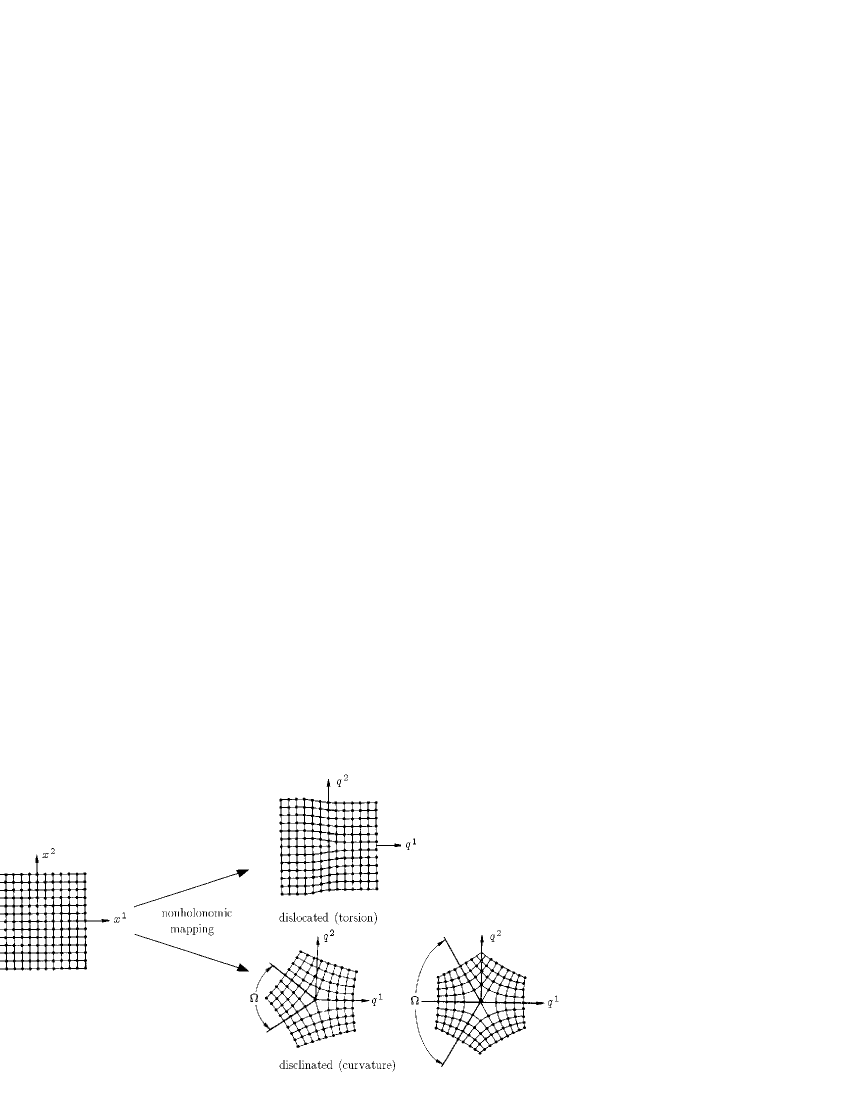
FIG. 1.:

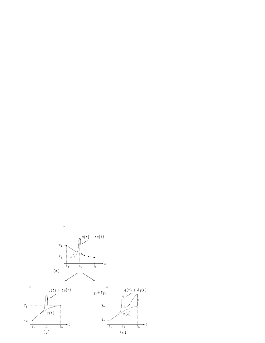
FIG. 2.:

REFERENCES

-
[1]
B.S. DeWitt, Rev. Mod. Phys. 29, 337 (1957).
His work makes use of the semiclassical amplitude by C. DeWitt-Morette, Phys. Rev. 81, 848 (1951). - [2] B. Podolsky, Phys. Rev. 32, 812 (1929).
-
[3]
K.S. Cheng, J. Math. Phys. 13, 1723 (1972),
who has an extra -term. See also related problems in
H. Kamo and T. Kawai, Prog. Theor. Phys. 50, 680 (1973); M.B. Menskii, Theor. Math. Phys 18, 190 (1974);
T. Kawai, Found. Phys. 5, 143 (1975);
M.M. Mizrahi, J. Math. Phys. 16, 2201 (1975);
M. Omote, Nucl. Phys. B 120, 325 (1977);
H. Dekker, Physica A 103, 586 (1980);
G.M. Gavazzi, Nuovo Cimento 101A, 241 (1981);
M. Böhm and G. Junker, J. Math. Phys. 28, 1978 (1987); C. Grosche and F. Steiner, J. Math. Phys. 36, 2354 (1995).
The last reference gives the most elaborate study of different discretizations, A Schrödinger equation without an additional -term is ensured by an a posteriori addition of appropriate nonclassical terms to the short-time action. A review on a variety of ambiguous attempts at quantizing such systems is given in the article by
M.S. Marinov, Physics Reports 60, 1 (1980).
A measure in the phase space formulation of path integrals which avoids an -term was found by
K. Kuchar, J. Math. Phys. 24, 2122 (1983).
-
[4]
Among the most widely discussed procedures was a
postpoint discretization due to Ito
and a midpoint discretization due to Stratonovich,
with different mathematical
advantages.
For a detailed discussion see
the textbooks
H. Risken, The Fokker-Planck Equation, ibid., 1983, Vol. 18;
R. Kubo, M. Toda, and N. Hashitsume, Statistical Physics II, Springer, Berlin, 1985. A recent description of the relation between time slicing and Ito versus Stratonovich calculus can be found in
H. Nakazato, K. Okano, L. Schülke, and Y. Yamanaka, Nucl. Phys. B 346, 611 (1990).
Stochastic differential equations in curved spaces are developed in
K.D. Elworthy, Stochastic differential equations on manifolds Cambridge Univ. Press, 1982;
M. Emery, Stochastic calculus in manifolds, Springer, Berlin, 1989. -
[5]
The basic observation underlying path integrals for time evolution
amplitudes
goes back to the historic article
P.A.M. Dirac, Physikalische Zeitschrift der Sowjetunion 3, 64 (1933).
He observed that the short-time propagator is the exponential of times the classical action. See also
P.A.M. Dirac, The Principles of Quantum Mechanics, Oxford University Press, Oxford, 1947,
and
E.T. Whittaker, Proc. Roy. Soc. Edinb. 61, 1 (1940).
Path integrals in configuration space were invented by R. P. Feynman in his 1942 Princeton thesis. The theory was published in 1948 in
R.P. Feynman, Rev. Mod. Phys. 20, 367 (1948).
- [6] L.D. Landau and E.M. Lifshitz, Quantum Mechanics, Pergamon, New York, 1965.
-
[7]
D.J. Simms and N. M. J. Woodhouse,
Lectures on geometric quantization,
Springer, Berlin, 1976;
J. Sniatycki, Geometric quantization and quantum mechanics, Springer, Berlin, 1980;
P.L. Robinson and J.H. Rawnsley, The metaplectic representation, Mpc structures, and geometric quantization, publ. by the American Mathematical Society in the series Memoirs of the American Mathematical Society no. 410 0065-9266, Providence, R.I., 1989.
Compare also
K.D. Elworthy, Path Integration on Manifolds, in Mathematical Aspects of Superspace, eds. H.-J. Seifert, C. Clarke, and A. Rosenblum, Reidel, 1984. - [8] H. Duru and H. Kleinert, Phys. Lett. B 84, 185 (1979); Fortschr. d. Phys. 30, 401 (1982).
-
[9]
H. Kleinert,
Path Integrals in Quantum Mechanics,
Statistics and Polymer Physics,
World Scientific, Singapore 1995. - [10] H. Kleinert, Mod. Phys. Lett. A 4, 2329 (1989);
- [11] H. Kleinert, Phys. Lett. B 236, 315 (1990).
- [12] The details are shown in Appendix 11A of Ref. [9].
- [13] P. Fiziev and H. Kleinert, New Action Principle for Classical Particle Trajectories In Spaces with Torsion, Berlin preprint (hep-th/9503074).
- [14] P. Fiziev and H. Kleinert, Euler Equations for Rigid-Body — A Case for Autoparallel Trajectories in Spaces with Torsion, Berlin preprint (hep-th/9503075).
-
[15]
H. Kleinert, Collective Quantum Fields,
Lectures presented at the First Erice Summer School on Low-Temperature Physics, 1977, Fortschr. Physik 26, 565-671 (1978).
See also the predecessors:
H. Kleinert, Field Theory of Collective Excitations — A Solvable Model,
Phys. Lett. B 69, 9 (1977). -
[16]
For a review on pairing forces:
D.R. Bes, R.A. Broglia, Lectures delivered at “E. Fermi” Varenna Summer School, Varenna, Como Italy, 1976;
D.R. Bes, R.A. Broglia, R. Liotta, B.R. Mottelson, Phys. Letters B 52, 253 (1974); B 56, 109 (1975); Nuclear Phys. A 260, 127 (1976);
R.W. Richardson, J. Math. Phys. 9, 1329 (1968), Ann. Phys. (N.Y.) 65, 249 (1971), and N.Y.U. Preprint 1977,
as well as references therein. - [17] L.P. Gorkov, Sov. Phys. JETP 9, 1364 (1959).
- [18] V.L. Ginzburg and L.D. Landau, Eksp. Teor. Fiz. 20, 1064 (1950).
-
[19]
For the derivation of an SU(3)SU(3) chirally invariant
collective quantum field theory
of mesons from a quark theory see
H. Kleinert, Hadronization of Quark Theories and a Bilocal form of QED,
Phys. Lett. B 62, 429 (1976);
H. Kleinert, On the Hadronization of Quark Theories, Lectures presented at the Erice Summer Institute 1976, in Understanding the Fundamental Constituents of Matter, Plenum Press, New York, 1978, A. Zichichi ed., pp. 289-390.
The recent status is summarized in
D. Blaschke, Path Integral Approach to Effective QCD at Finite Temperatures, Lecture presented at the 5th International Conference on Path Integrals from meV to MeV in Dubna, May 26-31, 1996. Proceedings in press. - [20] A.L. Leggett, Rev. Mod. Phys. 47, 331 (1975)
-
[21]
See also:
K.D. Schotte and U. Schotte, Phys. Rev. 182, 479 (1969);
S. Tomonaga, Progr. Theor. Phys. 5, 63 (1950) - [22] J. Hubbard, Phys. Rev. Letters 3, 77 (1959); B. Mühlschlegel, J. Math. Phys. , 3, 522 (1962); J. Langer, Phys. Rev. A 134, 553 (1964); T.M. Rice, Phys. Rev. A 140 1889 (1965); J. Math. Phys. 8, 1581 (1967); A.V. Svidzinskij, Teor. Mat. Fiz. 9, 273 (1971); D. Sherrington, J. Phys. C 4, 401 (1971).
-
[23]
E. Witten, Commun. Math. Phys. 92, 455 (1984);
P. DiVecchia and P. Rossi, Phys. Lett. B 140, 344 (1984);
P. DiVecchia, B. Durhuus and J.L. Petersen, Phys. Lett. B 144, 245 (1984);
Y. Frishman, Phys. Lett. B 146, 204 (1984);
E. Abdalla and M.C.B. Abdalla, Nucl. Phys. B 225, 392 (1985);
D. Gonzales and A.N. Redlich, Phys. Lett. B 147, 150 (1984);
C.M. Naón, Phys. Rev. D 31, 2035 (1985);
See also the recent development by
P.H. Damgaard, H.B. Nielsen, and R. Sollacher, Nuclear Phys. B 385, 227 (1992) (hep-th/9407022);
P.H. Damgaard and R. Sollacher, Cern preprint (hep-th/9407022);
A.N. Theron; F.A. Schaposnik,and H.B. Geyer, Nucl. Phys. B 437, 187 (1995) (hep-th/9410035);
C.P. Burgess and F. Quevedo, Phys. Lett. B 329 (1994) 457; Nucl. Phys. B 421, 373 (1994);
C.P. Burgess, A. Lutkin, and F. Quevedo, Phys. Lett. B 336, 18 (1994);
J. Fröhlich, R. Götschmann and P.A. Marchetti, preprint (hep-th/9406154); -
[24]
S. Coleman, Phys. Rev. D 11, 2088 (1975);
S. Mandelstam, Phys. Rev. D 11, 3026 (1975);
B. Schroer and T.T. Truong, Phys. Rev. D 15, 1684 (1977). -
[25]
For details and more references see
H. Kleinert, Gauge Fields in Condensed Matter, Vol. I Superflow and Vortex Lines,
pp. 1–744. and Vol. II Stresses and Defects,
World Scientific Publishing Co., Singapore 1989, pp. 744-1443. -
[26]
K. Kondo, in: Proc. 2nd Japan Nat. Congr. Applied Mechanics,
Tokio, 1952
B.A. Bilby, R. Bullough and E. Smith, Proc. R. Soc. London A231, 263 (1955);
E. Kröner, in: Physics of defects, Les Houches summer school XXXV, North-Holland, Amsterdam 1981; -
[27]
For a semiclassical study of the model at finite times see
H. Kleinert and H. Reinhardt, Nucl. Phys. A 332, 33 (1979).
FIGURE HEADINGS