June 1996 PAR–LPTHE 96–17 and ITFA 96–16, hep-th/9606029
SPONTANEOUSLY BROKEN
ABELIAN CHERN-SIMONS THEORIES

Abstract

A detailed analysis of Chern-Simons (CS) theories in which a compact abelian direct product gauge group $U(1)^{k}$ is spontaneously broken down to a direct product of cyclic groups $H\simeq{\mbox{\bf Z}}_{N^{(1)}}\times\cdots\times{\mbox{\bf Z}}_{N^{(k)}}$ is presented. The spectrum features global $H$ charges, vortices carrying magnetic flux labeled by the elements of $H$ and dyonic combinations. Due to the Aharonov-Bohm effect these particles exhibit topological interactions. The remnant of the $U(1)^{k}$ CS term in the discrete ${H}$ gauge theory describing the effective long distance physics of such a model is shown to be a 3-cocycle for ${H}$ summarizing the nontrivial topological interactions for the magnetic fluxes implied by the ${U(1)^{k}}$ CS term. It is noted that there are in general three types of 3-cocycles for a finite abelian gauge group ${H}$: one type describes topological interactions between vortices carrying flux w.r.t. the same cyclic group in the direct product $H$, another type gives rise to topological interactions among vortices carrying flux w.r.t. two different cyclic factors of $H$ and a third type leading to topological interactions between vortices carrying flux w.r.t. three different cyclic factors. Among other things, it is demonstrated that only the first two types can be obtained from a spontaneously broken $U(1)^{k}$ CS theory. The 3-cocycles that can not be reached in this way turn out to be the most interesting. They render the theory nonabelian and in general lead to dualities with planar theories with a nonabelian finite gauge group. In particular, the CS theory with finite gauge group $H\simeq{\mbox{\bf Z}}_{2}\times{\mbox{\bf Z}}_{2}\times{\mbox{\bf Z}}_{2}$ defined by such a 3-cocycle is shown to be dual to the planar discrete $D_{4}$ gauge theory with $D_{4}$ the dihedral group of order 8.

1 Introduction

A characteristic feature of 2+1 dimensional space time is the possibility to endow a gauge theory with a Chern-Simons (CS) term. Ever since the pioneering work by Schonfeld and Deser, Jackiw and Templeton [1] in the early eighties, these topological terms have had an impact in various seemingly unrelated branches of physics and mathematics. Notably, in a seminal paper [2] Witten pointed out the significance of pure CS theories in the setting of knot invariants and in so doing revealed a deep connection between pure CS theory and 1+1 dimensional rational conformal field theory. Earlier on, it was demonstrated by Hagen and Arovas, Schrieffer and Wilczek [4] that sources coupled to abelian CS gauge fields in general behave as anyons [3], i.e. particles with fractional spin and quantum statistics intermediate between bosons and fermions. Anyons and CS theories gained further attention after it was shown that an ideal gas of anyons is superconducting [5]. Moreover, it is by know well-established that anyons are realized in nature as quasi-particles in fractional quantum Hall liquids [6]. This remarkable observation due to Lauglin and the aforementioned general results initiated a large body of work in which fractional quantum Hall systems have served as a playground for applications of 1+1 dimensional conformal field theory and 2+1 dimensional CS theories (e.g. [7] and references therein). Finally, CS theory also plays a role in 2+1 dimensional gravity [8].

In this paper, the main focus is on the implications of adding a CS term to planar gauge theories which are spontaneously broken down to a finite residual gauge group via the Higgs mechanism. That is, the models under consideration are governed by an action of the form

$$S = S_{\mbox{\scriptsize YMH}}+S_{\mbox{\scriptsize matter}}+S_{\mbox{\scriptsize CS}}\,,$$ (1.1)

where the Yang-Mills Higgs action $S_{\rm{\mbox{\scriptsize YMH}}}$ gives rise to the spontaneous breakdown of some continuous compact gauge group $G$ to a finite subgroup ${H}$ and $S_{\mbox{\scriptsize matter}}$ describes a conserved matter current minimally coupled to the gauge fields. Finally, $S_{\mbox{\scriptsize CS}}$ denotes the CS action for the gauge gauge fields.

The discrete $H$ gauge theories describing the long distance physics of the models (1.1) without CS term $S_{\mbox{\scriptsize CS}}$ for the broken gauge group $G$ have been studied by various authors both in 2+1 and 3+1 dimensional space time and are by now completely understood. (For a recent detailed treatment and an up to date account of the literature on these models, the interested reader is referred to the lecture notes [9].) The spectrum features topological defects which in 2+1 dimensional space time appear as (particle-like) vortices carrying magnetic flux labeled by the elements of the finite gauge group $H$. In case $H$ is nonabelian, the vortices generally exhibit a nonabelian Aharonov-Bohm (AB) effect [10]: upon braiding two vortices their fluxes affect each other through conjugation [11]. Under the action of the residual global gauge group $H$, the fluxes also transform through conjugation and the conclusion is that the different magnetic vortices are labeled by the conjugacy classes of $H$. This is in a nutshell the physics described by the Yang-Mills Higgs part $S_{\mbox{\scriptsize YMH}}$ of the action (1.1). The matter fields, covariantly coupled to the gauge fields in the matter part $S_{\mbox{\scriptsize matter}}$ of the action, form multiplets which transform irreducibly under the broken gauge group ${G}$. In the broken phase, these branch to irreducible representations of the residual gauge group ${H}$. So, the matter fields introduce point charges in the broken phase labeled by the unitary irreducible representations (UIR’s) $\Gamma$ of $H$. If such a charge encircles a magnetic flux $h\in H$, it also undergoes an AB effect [12, 13, 14]. That is, it returns transformed by the matrix $\Gamma(h)$ assigned to the group element $h$ in the representation $\Gamma$ of $H$. Since the gauge fields in these models are completely massive, the foregoing topological AB effects form the only long range interactions among the charges and vortices. Of course, the complete spectrum also features the dyons obtained by composing the vortices and charges. These are labeled by the conjugacy classes of $H$ paired with a nontrivial centralizer representation [15]. Finally, as has been pointed out in reference [15] as well, this spectrum of charges, vortices and dyons and the spin, braiding and fusion properties of these particles is fully described by the representation theory of the quasitriangular Hopf algebra $D(H)$ resulting [16] from Drinfeld’s double construction [17] applied to the abelian algebra ${\cal F}(H)$ of functions on the finite group ${H}$.

The presence of a CS term $S_{\mbox{\scriptsize CS}}$ for the broken gauge group $G$ in the action (1.1) naturally has a bearing on the long distance physics. In [18, 19], it was argued on general grounds that the remnant of a CS term in the discrete $H$ gauge theory describing the long distance physics of the model is a 3-cocycle $\omega\in H^{3}(H,U(1))$ for the residual finite gauge group $H$, which governs the additional AB interactions among the vortices implied by the original CS term $S_{\mbox{\scriptsize CS}}$ for the broken gauge group $G$. Accordingly, the related algebraic structure now becomes the quasi-Hopf algebra $D^{\omega}(H)$ being a natural deformation of $D(H)$ depending on this 3-cocycle $\omega$. These general results were just explicitly illustrated by the example of the abelian CS Higgs model in which the (compact) gauge group $G\simeq U(1)$ is broken down to a cyclic subgroup $H\simeq{\mbox{\bf Z}}_{N}$. In the present paper, this analysis is extended to the general case of spontaneously broken abelian CS theories (1.1). That is, we will concentrate on symmetry breaking schemes

$${G}\;\simeq\;U(1)^{k} \longrightarrow {H}\,,$$ (1.2)

with $U(1)^{k}$ being the direct product of $k$ compact $U(1)$ gauge groups and the finite subgroup $H$ a direct product of $k$ cyclic groups ${\mbox{\bf Z}}_{N^{(i)}}$ of order $N^{(i)}$

$${H} \simeq {\mbox{\bf Z}}_{N^{(1)}}\times{\mbox{\bf Z}}_{N^{(2)}}\times\cdots\times{\mbox{\bf Z}}_{N^{(k)}}\,.$$ (1.3)

One of the main aims is to give a complete classification of these broken abelian planar gauge theories.

In fact, unbroken CS theory with direct product gauge group $U(1)^{k}$ endowed with minimally coupled matter fields has received considerable attention recently (e.g. [20, 21] and references therein). One of the motivations to study these theories is that they find an application in multi-layered quantum Hall systems. To give a brief sketch of the main results, the CS terms for the gauge group $U(1)^{k}$ are known to fall into two types. On the one hand, there are CS terms (type I) that describe self-couplings of the various $U(1)$ gauge fields. On the other hand, there are terms (type II) that establish couplings between two different $U(1)$ gauge fields. To be concrete, the most general CS action for the gauge group $G\simeq U(1)\times U(1)$, for instance, is of the form

$$S_{\mbox{\scriptsize CS}} = \int d\,^{3}x\;\left(\,\frac{\mu^{(12)}}{2}\epsilon^{\kappa\sigma\rho}A^{(1)}_{\kappa}\partial_{\sigma}A^{(2)}_{\rho}\>+\>\sum_{i=1}^{2}\frac{\mu^{(i)}}{2}\epsilon^{\kappa\sigma\rho}A^{(i)}_{\kappa}\partial_{\sigma}A^{(i)}_{\rho}\,\right),$$ (1.4)

with $A_{\kappa}^{(1)}$ and $A_{\kappa}^{(2)}$ the two $U(1)$ gauge fields and $\epsilon^{\kappa\sigma\rho}$ the three dimensional anti-symmetric Levi-Civita tensor normalized such that $\epsilon^{012}=1$. The parameters $\mu^{(1)}$ and $\mu^{(2)}$ denote the topological masses characterizing the CS actions of type I and $\mu^{(12)}$ the topological mass characterizing the CS action of type II. In the unbroken phase, these CS terms assign magnetic fluxes to the quantized matter charges $q^{(1)}$ and $q^{(2)}$ coupled to the two compact $U(1)$ gauge fields. Specifically, the type I CS term for the gauge field $A_{\kappa}^{(i)}$ attaches a magnetic flux $\phi^{(i)}=-q^{(i)}/\mu^{(i)}$ to a matter charge $q^{(i)}=n^{(i)}e^{(i)}$ with $n^{(i)}\in{\mbox{\bf Z}}$ and $e^{(i)}$ the coupling constant for $A_{\kappa}^{(i)}$. As a consequence, there are nontrivial topological AB interactions among these charges. When a charge $q^{(i)}$ encircles a remote charge $q^{(i)^{\prime}}$ in a counterclockwise fashion, the wave function acquires [22] the AB phase $\exp(-\imath q^{(i)}q^{(i)^{\prime}}/\mu^{(i)})$. The CS term of type II, in turn, attaches fluxes which belong to one $U(1)$ gauge group to the matter charges of the other. That is, a charge $q^{(1)}$ induces a flux $\phi^{(2)}=-2q^{(1)}/\mu^{(12)}$ and a charge $q^{(2)}$ induces a flux $\phi^{(1)}=-2q^{(2)}/\mu^{(12)}$. Hence, the type II CS term gives rise to topological interactions among matter charges of the two different $U(1)$ gauge groups [20]. A counterclockwise monodromy of a charge $q^{(1)}$ and a charge $q^{(2)}$, for example, yields the AB phase $\exp(-2\imath q^{(1)}q^{(2)}/\mu^{(12)})$.

The spontaneously broken versions (1.2) of these abelian CS theories, however, have not yet been fully explored. Among other things, I will argue that in the broken case the $U(1)^{k}$ CS term gives rise to nontrivial AB phases among the vortices labeled by the elements of the residual gauge group (1.3). To be specific, the $k$ different vortex species carry quantized flux $\phi^{(i)}=\frac{2\pi a^{(i)}}{N^{(i)}e^{(i)}}$ with $a^{(i)}\in{\mbox{\bf Z}}$ and $N^{(i)}$ the order of the $i^{\rm th}$ cyclic group of the product group (1.3). A type I CS term for the gauge field $A_{\kappa}^{(i)}$ then implies the AB phase $\exp(\imath\mu^{(i)}\phi^{(i)}\phi^{(i)^{\prime}})$ for a counterclockwise monodromy of a vortex $\phi^{(i)}$ and a vortex $\phi^{(i)^{\prime}}$. A CS term of type II coupling the gauge fields $A_{\kappa}^{(i)}$ and $A_{\kappa}^{(j)}$, in turn, gives rise to the AB phase $\exp(\imath\mu^{(ij)}\phi^{(i)}\phi^{(j)})$ for the process in which a vortex $\phi^{(i)}$ circumnavigates a vortex $\phi^{(j)}$ in a counterclockwise fashion. In agreement with the general remarks in an earlier paragraph, these additional AB phases among the vortices are shown to be the only distinction with the abelian discrete $H$ gauge theory describing the long distance physics in the absence of a CS action for the broken gauge group $U(1)^{k}$. That is, as was already pointed out for the simplest case $U(1)\rightarrow{\mbox{\bf Z}}_{N}$ in [14, 18, 19], the Higgs mechanism removes the fluxes attached the matter charges $q^{(i)}$ in the unbroken CS phase. Hence, contrary to the unbroken CS phase, there are no AB interactions among the matter charges in the CS Higgs phase. The canonical AB interactions $\exp(\imath q^{(i)}\phi^{(i)})$ between the matter charges $q^{(i)}$ and the magnetic vortices $\phi^{(i)}$ persist though.

A key role in the analysis of this paper is played by the Dirac monopoles [23] that can be introduced in these compact $U(1)^{k}$ CS theories. There are $k$ different species corresponding to the $k$ different compact $U(1)$ gauge groups. It is known [21, 24, 25] that a consistent incorporation of these monopoles requires the quantization of the topological masses characterizing the type I and type II CS terms. Moreover, it has been argued that in contrast to ordinary 2+1 dimensional compact QED [26], the presence of Dirac monopoles does not lead to confinement of the charges $q^{(i)}$ in the unbroken CS phase [25, 27, 28]. Instead, the monopoles in these CS theories describe tunneling events leading to the creation or annihilation of charges $q^{(i)}$ with magnitude depending on the integral CS parameter. That is, the spectrum just features a finite number of stable charges depending on the integral CS parameter [19, 21, 28]. As usual, the presence of Dirac monopoles in the broken phase implies that the magnetic fluxes $a^{(i)}$ carried by the vortices are conserved modulo $N^{(i)}$, but the flux decay driven by the monopoles is now accompanied by the creation of matter charge where the species of the charge depends on the type of the CS term and the magnitude is again proportional to the integral CS parameter (see also [18, 19]). Finally, it is shown that the quantization of topological mass implied by the presence of Dirac monopoles is precisely such that the $U(1)^{k}$ CS terms indeed boil down to a 3-cocycle for the residual finite gauge group $H$ in the broken phase.

The organization of this paper is as follows. In section 2, I start by briefly recalling a result due to Dijkgraaf and Witten [29] stating that the different CS actions $S_{\mbox{\scriptsize CS}}$ for a compact gauge group $G$ are labeled by the elements of the cohomology group $H^{4}(BG,{\mbox{\bf Z}})$ of the classifying space $BG$. A classification which for finite groups $H$ boils down to the cohomology group $H^{3}(H,U(1))$ of the group $H$ itself. In other words, the different CS theories for a finite gauge group $H$ correspond to the inequivalent 3-cocycles $\omega\in H^{3}(H,U(1))$. The new observation in this section is that the effective long distance physics of a CS theory in which the gauge group $G$ is broken down to a finite subgroup $H$ via the Higgs mechanism is described by a discrete $H$ CS theory defined by the 3-cocycle $\omega\in H^{3}(H,U(1))$ determined by the original CS action $S_{\mbox{\scriptsize CS}}\in H^{4}(BG,{\mbox{\bf Z}})$ for the broken gauge group $G$ through the natural homomorphism $H^{4}(BG,{\mbox{\bf Z}})\rightarrow H^{3}(H,U(1))$ induced by the inclusion $H\subset G$. Section 3 subsequently contains a short introduction to the cohomology groups $H^{n}(H,U(1))$ of finite abelian groups $H$. In particular, the explicit realization of the complete set of independent 3-cocycles $\omega\in H^{3}(H,U(1))$ for the abelian groups (1.3) is presented there. It turns out that these split up into three different types, namely 3-cocycles (type I) which give rise to nontrivial AB interactions among fluxes of the same cyclic gauge group in the direct product (1.3), those (type II) that describe interactions between fluxes corresponding to two different cyclic gauge groups and finally 3-cocycles (type III) that lead to additional AB interactions between fluxes associated to three different cyclic gauge groups. Section 4 then deals with the classification of CS actions for the compact gauge group $U(1)^{k}$. As mentioned before, these come in two types: CS actions (type I) that describe self couplings of the different $U(1)$ gauge fields and CS action (type II) establishing pairwise couplings between different $U(1)$ gauge fields. The natural conclusion is that the homomorphism $H^{4}(B(U(1)^{k}),{\mbox{\bf Z}})\to H^{3}(H,U(1))$ induced by the spontaneous symmetry breakdown (1.2) is not onto. That is, the only CS theories with finite abelian gauge group (1.3) that may arise from a spontaneously broken $U(1)^{k}$ CS theory are those corresponding to a 3-cocycle of type I and/or type II, while 3-cocycles of type III do not occur.

Section 5 is devoted to a discussion of the quasi–Hopf algebra $D^{\omega}(H)$ related to an abelian discrete $H$ CS theory defined by the 3-cocycle $\omega\in H^{3}(H,U(1))$. The emphasis is on the unified description this algebraic framework gives of the spin, braid and fusion properties of the magnetic vortices, charges and dyons constituting the spectrum of such a discrete $H$ CS theory.

In the next sections, the foregoing general considerations are illustrated by some representative examples. Specifically, section 6 deals with the abelian CS Higgs model in which the compact gauge group $G\simeq U(1)$ is broken down to the cyclic subgroup $H\simeq{\mbox{\bf Z}}_{N}$. First, the unbroken $U(1)$ phase of this model is briefly reviewed. In particular, it is recalled that a consistent implementation of Dirac monopoles requires the topological mass to be quantized as $\mu=\frac{pe^{2}}{\pi}$ with $p\in{\mbox{\bf Z}}$ and $e$ the coupling constant, which is in agreement with the fact that the different CS actions for a compact gauge group $U(1)$ are classified by the integers: $H^{4}(BU(1),{\mbox{\bf Z}})\simeq{\mbox{\bf Z}}$. Subsequently, the broken phase of the model is discussed. Among other things, it is established that the long distance physics is indeed described by a ${\mbox{\bf Z}}_{N}$ CS theory with 3-cocycle $\omega\in H^{3}({\mbox{\bf Z}}_{N},U(1))\simeq{\mbox{\bf Z}}_{N}$ fixed by the natural homomorphism $H^{4}(BU(1),{\mbox{\bf Z}})\to H^{3}({\mbox{\bf Z}}_{N},U(1))$. In other words, the integral CS parameter $p$ becomes periodic in the broken phase with period $N$. Section 7 then contains a similar treatment of a CS theory of type II with gauge group $G\simeq U(1)\times U(1)$ spontaneously broken down to $H\simeq{\mbox{\bf Z}}_{N^{(1)}}\times{\mbox{\bf Z}}_{N^{(2)}}$. The effective long distance physics of this model is described by a ${\mbox{\bf Z}}_{N^{(1)}}\times{\mbox{\bf Z}}_{N^{(2)}}$ CS theory defined by a 3-cocycle of type II. The abelian discrete $H$ CS theories which do not occur as the remnant of a spontaneously broken $U(1)^{k}$ CS theory are actually the most interesting. These are the CS theories defined by the aforementioned 3-cocycles of type III. The simplest example of such a theory, namely that with gauge group $H\simeq{\mbox{\bf Z}}_{2}\times{\mbox{\bf Z}}_{2}\times{\mbox{\bf Z}}_{2}$, is treated in full detail in section 8. It is pointed out that the incorporation of the corresponding 3-cocycle of type III renders the theory nonabelian. That is, the resulting type III CS theory exhibits nonabelian phenomena like Alice fluxes, Cheshire charges, nonabelian Aharonov-Bohm sacttering and the multi-particle configurations generally satisfy nonabelian braid statistics. Probably the most striking result of this section is that this theory turns out to be dual to the ordinary $D_{4}$ planar gauge theory with $D_{4}$ the nonabelian dihedral group of order $8$. Moreover, it is argued that the ${\mbox{\bf Z}}_{2}\times{\mbox{\bf Z}}_{2}\times{\mbox{\bf Z}}_{2}$ CS theory defined by the product of the 3-cocycle of type III and either one of the three 3-cocycles of type I is dual to the ordinary $\bar{D}_{2}$ planar gauge theory with $\bar{D}_{2}$ the quaternion group being the other nonabelian group of order $8$.

Finally, section 9 presents some new results on the Dijkgraaf-Witten invariant for lens spaces based on the three different types of 3-cocycles for various finite abelian groups $H$, whereas some concluding remarks and an outlook can be found in section 10.

In addition, there are three appendices. In appendix A, I have collected the derivation of some identities in the theory of group cohomology used in the main text. In particular, it contains a derivation of the content of the cohomology group $H^{3}(H,U(1))$ for an arbitrary abelian finite group $H$ of the form (1.3) and a derivation of the content of the cohomology group $H^{4}(B(U(1)^{k}),{\mbox{\bf Z}})$. Further, one of the novel observations in this paper is that rather than representations of the ordinary braid groups the multi-particle systems in abelian discrete $H$ CS theories realize representations of so-called truncated braid groups being factor groups of the ordinary braid groups. The precise definition of these truncated braid groups is given in appendix B along with useful identifications of some of them with well-known finite groups. Finally, the characteristic features of a planar gauge theory with finite nonabelian gauge group the dihedral group $D_{4}$ (being dual to the ${\mbox{\bf Z}}_{2}\times{\mbox{\bf Z}}_{2}\times{\mbox{\bf Z}}_{2}$ CS theory defined by a 3-cocycle of type III as argued in section 8.3) are briefly discussed in appendix C.

In passing, the treatment of the examples in sections 6, 7 and 8 is more or less self contained. So, the more physically inclined reader who may not be so much interested in the rather mathematical classification side of the problem could well start with section 6 and occasionally go back to earlier sections for definitions and technicalities.

As for conventions, throughout this paper natural units in which $\hbar=c=1$ are employed. We will exclusively work in 2+1 dimensional Minkowsky space with signature $(+,-,-)$. Spatial coordinates are denoted by $x^{1}$ and $x^{2}$ and the time coordinate by $x^{0}=t$. As usual, greek indices run from 0 to 2, while spatial components are labeled by latin indices$\in 1,2$. Unless stated otherwise, we will use Einstein’s summation convention.

2 Group cohomology and symmetry breaking

As has been argued by Dijkgraaf and Witten [29], the CS actions $S_{\mbox{\scriptsize CS}}$ for a compact gauge group $G$ are in one-to-one correspondence with the elements of the cohomology group $H^{4}(B{G},{\mbox{\bf Z}})$ of the classifying space $B{G}$ with integer coefficients Z.  In particular, this classification includes the case of finite gauge groups $H$. The isomorphism [31]

$$H^{n}(B{H},{\mbox{\bf Z}}) \simeq H^{n}({H},{\mbox{\bf Z}})\,,$$ (2.1)

which only holds for finite groups ${H}$, shows that the cohomology of the classifying space $BH$ is the same as that of the group $H$ itself. In addition, we have the isomorphism

$$H^{n}(H,{\mbox{\bf Z}}) \simeq H^{n-1}({H},U(1))\qquad\forall\,n>1\,.$$ (2.2)

A derivation of this result, using the universal coefficients theorem, is contained in appendix A. Especially, we now arrive at the identification

$$H^{4}({BH},{\mbox{\bf Z}}) \simeq H^{3}({H},U(1))\,,$$ (2.3)

which expresses the fact that the different CS theories for a finite gauge group $H$ are, in fact, defined by the different elements $\omega\in H^{3}({H},U(1))$, i.e. algebraic 3-cocycles $\omega$ taking values in $U(1)$. These 3-cocycles can be interpreted as $\omega=\exp(\imath S_{\mbox{\scriptsize CS}})$, where $S_{\mbox{\scriptsize CS}}$ denotes a CS action for the finite gauge group $H$ [29]. With abuse of language, we will usually call $\omega$ itself a CS action for $H$.

Let $K$ be a subgroup of a compact group $G$. The inclusion $K\subset G$ induces a natural homomorphism

$$H^{4}(B{G},{\mbox{\bf Z}}) \longrightarrow H^{4}(BK,{\mbox{\bf Z}})\,,$$ (2.4)

called the restriction (e.g. [32]). This homomorphism determines the fate of a given CS action $S_{\mbox{\scriptsize CS}}\in H^{4}(B{G},{\mbox{\bf Z}})$ when the gauge group $G$ is spontaneously broken down to $K$ via the Higgs mechanism. That is, the mapping (2.4) fixes the CS action $\in H^{4}(BK,{\mbox{\bf Z}})$ for the residual gauge group $K$ to which $S_{\mbox{\scriptsize CS}}$ reduces in the broken phase. In the following, we will only be concerned with CS theories in which a continuous (compact) gauge group $G$ is broken down to a finite subgroup $H$. The long distance physics of such a model is described by a discrete $H$ CS theory with 3-cocycle $\omega\in H^{3}({H},U(1))$ determined by the original CS action $S_{\mbox{\scriptsize CS}}$ for the broken gauge group $G$ through the natural homomorphism

$$H^{4}(B{G},{\mbox{\bf Z}}) \longrightarrow H^{3}({H},U(1))\,,$$ (2.5)

being the composition of the restriction $H^{4}(B{G},{\mbox{\bf Z}})\to H^{4}(BH,{\mbox{\bf Z}})$ induced by the inclusion $H\subset G$, and the isomorphism (2.3). As will become clear in the following sections, the 3-cocycle $\omega$ governs the additional AB phases among the magnetic fluxes (labeled by the elements $h\in H$) in the broken phase implied by the CS action $S_{\mbox{\scriptsize CS}}$.

The restrictions (2.4) and (2.5) for continuous subgroups $K\subset G$ and finite subgroups $H\subset G$, respectively, are not necessarily onto. Hence, it is not guaranteed that all CS theories with continuous gauge group $K$ (or finite gauge group $H$) can be obtained from spontaneously broken CS theories with gauge group $G$. Particularly, in section 4, we will see that the natural homomorphism $H^{4}(B(U(1)^{k}),{\mbox{\bf Z}})\to H^{3}(H,U(1))$ induced by the symmetry breaking (1.2) is not onto.

3 Cohomology of finite abelian groups

In this section, I give a brief introduction to the cohomology groups $H^{n}({H},U(1))$ of a finite abelian group $H$. The plan is as follows. In subsection 3.1, I recall the basic definitions and subsequently focus on the cocycle structure occurring in an abelian discrete $H$ CS theory. Finally, subsection 3.2 contains the explicit realization of all independent 3-cocycles $\omega\in H^{3}({H},U(1))$ for an arbitrary abelian group ${H}$.

3.1 $H^{n}(H,U(1))$

In the (multiplicative) algebraic description of the cohomology groups $H^{n}(H,U(1))$ the $n$-cochains are represented as $U(1)$ valued functions

$$c:\;\underbrace{{H}\times\cdots\times{H}}_{n\;\mbox{\scriptsize times}} \longrightarrow U(1)\,.$$ (3.1)

The set of all $n$-cochains forms the abelian group $C^{n}({H},U(1)):=C^{n}$ with pointwise multiplication $(c\cdot d)\,(A_{1},\ldots,A_{n})=c\,(A_{1},\ldots,A_{n})\;d\,(A_{1},\ldots,A_{n}),$ where the capitals $A_{j}$ (with $1\leq j\leq n$) denote elements of the finite group ${H}$ and $c,d\in C^{n}$. The coboundary operator $\delta$ then establishes a mapping

$$\delta:\;C^{n} \longrightarrow C^{n+1}$$

$$c \longmapsto \delta c\,,$$

given by

$$\delta c\,(A_{1},\ldots,A_{n+1})\;:=$$

$$c\,(A_{2},\ldots,A_{n+1})\;c\,(A_{1},\ldots,A_{n})^{(-1)^{n+1}}\;\prod_{i=1}^{n}c\,(A_{1},\dots,A_{i}\cdot A_{i+1},\ldots,A_{n+1})^{(-1)^{i}}\,,$$

which acts as a derivation. That is, $\delta(c\cdot d)=\delta c\cdot\delta d$. It can be checked explicitly that $\delta$ is indeed nilpotent: $\delta^{2}=1$. The coboundary operator $\delta$ naturally defines two subgroups $Z^{n}$ and $B^{n}$ of $C^{n}$. Specifically, the subgroup $Z^{n}\subset C^{n}$ consists of $n$-cocycles being the $n$-cochains $c$ in the kernel of $\delta$

$$\delta c = 1\qquad\forall\,\,c\in Z^{n}\,,$$ (3.3)

whereas the subgroup $B^{n}\subset Z^{n}\subset C^{n}$ contains the $n$-coboundaries or exact $n$-cocycles

$$c = \delta b\qquad\forall\,\,c\in B^{n}\,.$$ (3.4)

with $b$ some cochain $\in C^{n-1}$. As usual, the cohomology group $H^{n}({H},U(1))$ is then defined as $H^{n}({H},U(1)):=Z^{n}/B^{n}$. In other words, the elements of $H^{n}({H},U(1))$ correspond to the different classes of $n$-cocycles (3.3) with equivalence relation $c\sim c\delta b$.

The so-called slant product $i_{A}$ with arbitrary but fixed $A\in H$ is a mapping in the opposite direction to the coboundary operator (e.g. [33])

$$i_{A}:\;C^{n} \longrightarrow C^{n-1}$$

$$c \longmapsto i_{A}c\,,$$

defined as

$$i_{A}c\,(A_{1},\ldots,A_{n-1})\;:=$$

$$c\,(A,A_{1},\ldots,A_{n-1})^{(-1)^{n-1}}\prod_{i=1}^{n-1}c\,(A_{1},\ldots,A_{i},A,A_{i+1},\ldots,A_{n-1})^{(-1)^{n-1+i}}\,.$$

It can be shown (e.g. [33]) that the slant product satisfies the relation $\delta(i_{A}c)=i_{A}\,\delta c$ for all $n$-cochains $c$. Notably, if $c$ is a $n$-cocycle, we immediately infer from this relation that $i_{A}c$ becomes a $(n-1)$-cocycle: $\delta(i_{A}c)=i_{A}\,\delta c=1$. Hence, the slant product establishes a homomorphism $i_{A}:H^{n}({H},U(1))\rightarrow H^{n-1}({H},U(1))$ for each $A\in H$.

Let us finally turn to the cocycle structure appearing in an abelian discrete $H$ gauge theory with CS action $\omega\in H^{3}({H},U(1))$. First of all, as indicated by (3.1) and (3.3), the 3-cocycle $\omega$ satisfies the relation

$$\omega(A,B,C)\;\omega(A,B\cdot C,D)\;\omega(B,C,D) = \omega(A\cdot B,C,D)\;\omega(A,B,C\cdot D)\,,\qquad$$ (3.6)

for all $A,B,C\in H$. To continue, the slant product (3.1) as applied to $\omega$ gives rise to a set of 2-cocycles $c_{A}\in H^{2}({H},U(1))$

$$c_{A}(B,C)\;:=\;i_{A}\omega(B,C)\;=\;\frac{\omega(A,B,C)\;\omega(B,C,A)}{\omega(B,A,C)}\,,$$ (3.7)

which are labeled by the different elements $A$ of $H$. As will become clear in section 5, these 2-cocycles enter the definition of the projective dyon charge representations associated to the magnetic fluxes in this abelian discrete $H$ CS gauge theory. To be specific, the different charges we can assign to a given abelian magnetic flux $A\in H$ to form dyons are labeled by the inequivalent unitary irreducible projective representations $\alpha$ of $H$ defined as

$${\alpha}(B)\,\cdot\,{\alpha}(C) = c_{A}(B,C)\;{\alpha}(B\cdot C)\,.$$ (3.8)

Here, the 2-cocycle relation satisfied by $c_{A}$

$$c_{A}(B,C)\;c_{A}(B\cdot C,D) = c_{A}(B,C\cdot D)\;c_{A}(C,D)\,,$$ (3.9)

implies that the representations $\alpha$ are associative. To conclude, as follows from (3.1) and (3.3), the 1-cocycles obey the relation $c\,(B)\;c\,(C)=c\,(B\cdot C)$. In other words, the different 1-cocycles being the elements of the cohomology group $H^{1}({H},U(1))$ correspond to the inequivalent ordinary UIR’s of the abelian group ${H}$. These label the conceivable free charges in a CS theory with finite abelian gauge group $H$.

3.2 Chern-Simons actions for finite abelian groups

An abstract group cohomological derivation (contained in appendix A) reveals the following results for the first three cohomology groups of the finite abelian group $H$ being the direct product ${\mbox{\bf Z}}_{N}^{k}$ of $k$ cyclic groups ${\mbox{\bf Z}}_{N}$ of order $N$

$$H^{1}({\mbox{\bf Z}}_{N}^{k},U(1)) \simeq {\mbox{\bf Z}}_{N}^{k}$$ (3.10)

$$H^{2}({\mbox{\bf Z}}_{N}^{k},U(1)) \simeq {\mbox{\bf Z}}_{N}^{\frac{1}{2}k(k-1)}$$ (3.11)

$$H^{3}({\mbox{\bf Z}}_{N}^{k},U(1)) \simeq {\mbox{\bf Z}}_{N}^{k+\frac{1}{2}k(k-1)+\frac{1}{3!}k(k-1)(k-2)}\,.$$ (3.12)

As we have seen in the previous subsection, the first result labels the inequivalent UIR’s of ${\mbox{\bf Z}}_{N}^{k}$, the second the different 2-cocycles entering the projective representations of ${\mbox{\bf Z}}_{N}^{k}$, and the last the number of different 3-cocycles or CS actions for ${\mbox{\bf Z}}_{N}^{k}$. The derivation of the isomorphism (3.12) in appendix A pointed out that there are, in fact, three dissimilar types of 3-cocycles. The explicit realization of these 3-cocycles involves some notational conventions which I establish first.

Let $A,B$ and $C$ denote elements of ${\mbox{\bf Z}}_{N}^{k}$, i.e.

$$A := (a^{(1)},a^{(2)},\ldots,a^{(k)})\qquad\mbox{with $a^{(i)}\in{\mbox{\bf Z}}_{N}$ for $i=1,\ldots,k$}\,,$$ (3.13)

and similar decompositions for $B$ and $C$. I adopt the additive presentation for the abelian group ${\mbox{\bf Z}}_{N}^{k}$, that is, the elements $a^{(i)}$ of ${\mbox{\bf Z}}_{N}$ take values in the range $0,\ldots,N-1$, and group multiplication is defined as

$$A\cdot B\;=\;[A+B]\;:=\;([a^{(1)}+b^{(1)}],\ldots,[a^{(k)}+b^{(k)}])\,.$$ (3.14)

Here, the rectangular brackets denote modulo $N$ calculus such that the sum always lies in the range $0,\ldots,N-1$. With these conventions, the three types of 3-cocycles for the direct product group ${\mbox{\bf Z}}_{N}^{k}$ can then be presented as

$$\halign to=0.0pt{\hskip\@centering$\displaystyle{#}$\@eqnsel&\global\@eqcnt\@ne\hskip\tw@\arraycolsep\hfil${#}$\hfil&\global\@eqcnt\tw@\hskip\tw@\arraycolsep$\displaystyle{#}$\hfil&\global\@eqcnt\thr@@\hskip\tw@\arraycolsep\hfil\hbox{#}&\global\@eqcnt 4 \hbox\bgroup\hss#\egroup\cr 0.0pt plus 1000.0pt$\displaystyle{\omega_{\rm I}^{(i)}(A,B,C) \!\!\! &10.0pt\hfil${=&10.0pt$\displaystyle{\!\!\! \exp\left( \frac{2 \pi\imath p^{(i)}_{\mbox{\scriptsize I}}}{N^{2}} a^{(i)}(b^{(i)} +c^{(i)} -[b^{(i)}+c^{(i)}]) \right) &10.0pt\hfil\hbox{$\!\!1\leq i\leq k$ \, \\ \omega_{\mbox{\scriptsize II}}^{(ij)}(A,B,C) \!\!\!&{\hss=}&\!\!\!\exp\left(\frac{2\pi\imath p^{(ij)}_{\mbox{\scriptsize II}}}{N^{2}}a^{(i)}(b^{(j)}+c^{(j)}-[b^{(j)}+c^{(j)}])\right)&$\!\! 1 \leq i < j \leq k$\,\\\omega_{\mbox{\scriptsize III}}^{(ijl)}(A,B,C)\!\!\!&=&\!\!\!\exp\left(\frac{2\pi\imath p^{(ijl)}_{\mbox{\scriptsize III}}}{N}a^{(i)}b^{(j)}c^{(l)}\right)&$\!\! 1 \leq i < j < l \leq k$,(3.15)\cr}}}}}$$

where the integral parameters $p_{\rm I}^{(i)}$, $p_{\mbox{\scriptsize II}}^{(ij)}$ and $p^{(ijl)}_{\mbox{\scriptsize III}}$ label the different elements of the cohomology group $H^{3}({\mbox{\bf Z}}_{N}^{k},U(1))$. In accordance with (3.12), the 3-cocycles are periodic functions of these parameters with period $N$. For the 3-cocycles of type III this periodicity is obvious, while for the 3-cocycles of type I and II it is immediate after the observation that the factors $(b^{(i)}+c^{(i)}-[b^{(i)}+c^{(i)}])$, with $1\leq i\leq k$, either vanish or equal $N$. It is also readily checked that the 3-cocycles (3.2)–(3.2) indeed satisfy the 3-cocycle relation (3.6).

The $k$ different 3-cocycles (3.2) of type I describe self-couplings, i.e. couplings between the magnetic fluxes ($a^{(i)}$,$b^{(i)}$ and $c^{(i)}$) associated to the same gauge group ${\mbox{\bf Z}}_{N}$ in the direct product ${\mbox{\bf Z}}_{N}^{k}$. In this counting procedure, it is, of course, understood that every 3-cocycle actually stands for a set of $N-1$ nontrivial 3-cocycles labeled by the periodic parameter $p_{\mbox{\scriptsize I}}^{(i)}$. The 3-cocycles (3.2) of type II, in turn, establish pairwise couplings between the magnetic fluxes corresponding to different gauge groups ${\mbox{\bf Z}}_{N}$ in the direct product ${\mbox{\bf Z}}_{N}^{k}$. Note that the 3-cocycles $\omega_{\mbox{\scriptsize II}}^{(ij)}$ and $\omega_{\mbox{\scriptsize II}}^{(ji)}$ are equivalent, since they just differ by a 3-coboundary (3.4). In other words, there are only $\frac{1}{2}k(k-1)$ distinct 3-cocycles of type II. A similar argument holds for the 3-cocycles (3.2) of type III. A permutation of the labels $i$, $j$ and $k$ in these 3-cocycles yields an equivalent 3-cocycle. Hence, we end up with $\frac{1}{3!}k(k-1)(k-2)$ different 3-cocycles of type III, which realize couplings between the fluxes associated to three distinct ${\mbox{\bf Z}}_{N}$ gauge groups in the direct product ${\mbox{\bf Z}}_{N}^{k}$.

We are now well prepared to discuss the 3-cocycle structure for general abelian groups $H$ being direct products (1.3) of cyclic groups possibly of different order. Let us assume that ${H}$ consists of $k$ cyclic factors. The abstract analysis in appendix A shows that depending on the divisibility of the orders of the different cyclic factors, there are again $k$ distinct 3-cocycles of type I, $\frac{1}{2}k(k-1)$ different 3-cocycles of type II and $\frac{1}{3!}k(k-1)(k-2)$ different 3-cocycles of type III. It is easily verified that the associated generalization of the 3-cocycle realizations (3.2), (3.2) and (3.2) becomes

$$\omega_{\mbox{\scriptsize I}}^{(i)}(A,B,C) = \exp\left(\frac{2\pi\imath p^{(i)}_{\mbox{\scriptsize I}}}{N^{(i)\;2}}\;a^{(i)}(b^{(i)}+c^{(i)}-[b^{(i)}+c^{(i)}])\right)$$ (3.16)

$$\omega_{\mbox{\scriptsize II}}^{(ij)}(A,B,C) = \exp\left(\frac{2\pi\imath p_{\mbox{\scriptsize II}}^{(ij)}}{N^{(i)}N^{(j)}}\;a^{(i)}(b^{(j)}+c^{(j)}-[b^{(j)}+c^{(j)}])\right)$$ (3.17)

$$\omega_{\mbox{\scriptsize III}}^{(ijl)}(A,B,C) = \exp\left(\frac{2\pi\imath p_{\mbox{\scriptsize III}}^{(ijl)}}{{\gcd}(N^{(i)},N^{(j)},N^{(l)})}\;a^{(i)}b^{(j)}c^{(l)}\right),$$ (3.18)

where $N^{(i)}$ (with $1\leq i\leq k$) denotes the order of the $i^{\rm th}$ cyclic factor of the direct product group $H$. In accordance with the isomorphism (A.28) of appendix A, the 3-cocycles of type III are cyclic in the integral parameter $p_{\mbox{\scriptsize III}}^{(ijl)}$ with period the greatest common divisor ${\gcd}(N^{(i)},N^{(j)},N^{(l)})$ of $N^{(i)}$, $N^{(j)}$ and $N^{(l)}$. The periodicity of the 3-cocycles of type I coincides with the order $N^{(i)}$ of the associated cyclic factor of $H$. Finally, the 3-cocycles of type II are periodic in the integral parameter $p_{\mbox{\scriptsize II}}^{(ij)}$ with period the greatest common divisor ${\gcd}(N^{(i)},N^{(j)})$ of $N^{(i)}$ and $N^{(j)}$. This last periodicity becomes clear upon using the chinese remainder theorem

$$\frac{\gcd(N^{(i)},N^{(j)})}{N^{(i)}N^{(j)}} = \frac{x}{N^{(i)}}+\frac{y}{N^{(j)}}\qquad\qquad\mbox{with $x,y\in{\mbox{\bf Z}}$}\,,$$ (3.19)

which indicates that (3.17) boils down to a 3-coboundary for $p_{\mbox{\scriptsize II}}^{(ij)}={\gcd}(N^{(i)},N^{(j)})$.

Let us finally focus on the 2-cocycles following from the three different types of 3-cocycles through the slant product (3.7). Upon substituting the expressions (3.16) and (3.17) in (3.7), we infer that the resulting 2-cocycles $c_{A}$ associated to the 3-cocycles of type I and II, respectively, correspond to the trivial element of the second cohomology group $H^{2}({H},U(1))$. To be precise, these 2-cocycles are 2-coboundaries

$$c_{A}(B,C)\;=\;\delta\varepsilon_{A}(B,C)\;=\;\frac{\varepsilon_{A}(B)\;\varepsilon_{A}(C)}{\varepsilon_{A}(B\cdot C)}\,,$$ (3.20)

where the 1-cochains $\varepsilon_{A}$ of type I and type II read

$$\varepsilon^{\mbox{\scriptsize I}}_{A}(B) = \exp\left(\frac{2\pi\imath p^{(i)}_{\mbox{\scriptsize I}}}{N^{(i)\,2}}\;a^{(i)}b^{(i)}\right)$$ (3.21)

$$\varepsilon^{\mbox{\scriptsize II}}_{A}(B) = \exp\left(\frac{2\pi\imath p^{(ij)}_{\mbox{\scriptsize II}}}{N^{(i)}N^{(j)}}\;a^{(i)}b^{(j)}\right).$$ (3.22)

Hence, the dyon charges in an abelian discrete $H$ gauge theory endowed with a CS action of type I and/or type II correspond to trivial projective representations (3.8) of $H$ of the form $\alpha=\varepsilon_{A}\Gamma$, where $\Gamma$ denotes an ordinary UIR of $H$. In contrast, the 2-cocycles $c_{A}$ obtained from the 3-cocycles (3.18) of type III correspond to nontrivial elements of the cohomology group $H^{2}({H},U(1))$. The conclusion is that the dyon charges featuring in an abelian discrete $H$ gauge theory with a CS action of type III are nontrivial (i.e. higher dimensional) projective representations of $H$.

4 Chern-Simons actions for $U(1)^{k}$ gauge theories

This section is concerned with the classification of the CS actions for the compact gauge group $U(1)^{k}$. In addition, it is established which CS theories with finite abelian gauge group $H$ may result from a spontaneous breakdown of the corresponding $U(1)^{k}$ CS theories.

As mentioned in the introduction, the most general CS action for a planar $U(1)^{k}$ gauge theory is of the form [20]

$$S_{\mbox{\scriptsize CS}} = \int d\,^{3}x\;({\cal L}_{\mbox{\scriptsize CSI}}+{\cal L}_{\mbox{\scriptsize CSII}})$$ (4.1)

$${\cal L}_{\mbox{\scriptsize CSI}} = \sum_{i=1}^{k}\;\frac{\mu^{(i)}}{2}\epsilon^{\kappa\sigma\rho}A^{(i)}_{\kappa}\partial_{\sigma}A^{(i)}_{\rho}$$ (4.2)

$${\cal L}_{\mbox{\scriptsize CSII}} = \sum_{i<j=1}^{k}\frac{\mu^{(ij)}}{2}\epsilon^{\kappa\sigma\rho}A^{(i)}_{\kappa}\partial_{\sigma}A^{(j)}_{\rho}\,,$$ (4.3)

where $A^{(i)}_{\kappa}$ (with $i=1,\dots,k$) denote the various $U(1)$ gauge fields, $\mu^{(i)}$, $\mu^{(ij)}$ the topological masses and $\epsilon^{\kappa\sigma\rho}$ the three dimensional anti-symmetric Levi-Civita tensor normalized such that $\epsilon^{012}=1$. Hence, there are $k$ distinct CS terms (4.2) describing self couplings of the $U(1)$ gauge fields. In analogy with the terminology developed in the previous section, we will call these terms CS terms of type I. In addition, there are $\frac{1}{2}k(k-1)$ distinct CS terms of type II establishing pairwise couplings between different $U(1)$ gauge fields. Note that by a partial integration a term labeled by $(ij)$ becomes a term $(ji)$. Therefore, these terms are equivalent and should not be counted separately. Also note that up to a total derivative the CS terms of type I and type II are indeed invariant under $U(1)^{k}$ gauge transformations $A^{(i)}_{\rho}\rightarrow A^{(i)}_{\rho}-\partial_{\rho}\Omega^{(i)}$ with $i=1,\ldots,k$, while the requirement of abelian gauge invariance immediately rules out ‘CS terms of type III’ $\sum_{i<j<l=1}^{k}\frac{\mu^{(ijl)}}{2}\epsilon^{\kappa\sigma\rho}A^{(i)}_{\kappa}A^{(j)}_{\sigma}A^{(l)}_{\rho}\,,$ which would establish a coupling between three different $U(1)$ gauge fields.

Let us now assume that this abelian gauge theory is compact and features a family of Dirac monopoles [23] for each compact $U(1)$ gauge group. That is, the complete spectrum of Dirac monopoles consists of the magnetic charges $g^{(i)}=\frac{2\pi m^{(i)}}{e^{(i)}}$ with $m^{(i)}\in{\mbox{\bf Z}}$, $1\leq i\leq k$ and $e^{(i)}$ the fundamental charge associated with the compact $U(1)$ gauge group being the $i^{\rm th}$ factor in the direct product $U(1)^{k}$. In this 2+1 dimensional Minkowsky setting, these monopoles are, of course, instantons tunneling between states with flux difference $\Delta\phi^{(i)}=\frac{2\pi m^{(i)}}{e^{(i)}}$. A consistent implementation of these monopoles/instantons requires that the topological masses in (4.2) and (4.3) are quantized as

$$\mu^{(i)} = \frac{p^{(i)}_{\mbox{\scriptsize I}}e^{(i)}e^{(i)}}{\pi}\;\qquad\qquad\mbox{with $p^{(i)}_{\mbox{\scriptsize I}}\in{\mbox{\bf Z}}$}$$ (4.4)

$$\mu^{(ij)} = \frac{p^{(ij)}_{\mbox{\scriptsize II}}e^{(i)}e^{(j)}}{\pi}\qquad\qquad\mbox{with $p^{(ij)}_{\mbox{\scriptsize II}}\in{\mbox{\bf Z}}$}\,.$$ (4.5)

This will be shown in sections 6.3 and 7.3, where we will discuss these models in further detail. The integral CS parameters $p^{(i)}_{\mbox{\scriptsize I}}$ and $p^{(ij)}_{\mbox{\scriptsize II}}$ now label the different elements of the cohomology group

$$H^{4}(B(U(1)^{k}),{\mbox{\bf Z}}) \simeq {\mbox{\bf Z}}^{k+\frac{1}{2}k(k-1)}\,,$$ (4.6)

where a derivation of the isomorphism (4.6) is contained in appendix A.

We now have all the ingredients to make explicit the homomorphism (2.5) accompanying the spontaneous symmetry breakdown of the gauge group $U(1)^{k}$ to the finite abelian group $H\simeq{\mbox{\bf Z}}_{N^{(1)}}\times\cdots\times{\mbox{\bf Z}}_{N^{(k)}}$. In terms of the integral CS parameters in (4.4) and (4.5), it takes the form

$$H^{4}(B(U(1)^{k}),{\mbox{\bf Z}}) \longrightarrow H^{3}({H},U(1))$$ (4.7)

$$p^{(i)}_{\mbox{\scriptsize I}} \longmapsto p^{(i)}_{\mbox{\scriptsize I}}\qquad\;\bmod N^{(i)}$$ (4.8)

$$p^{(ij)}_{\mbox{\scriptsize II}} \longmapsto p^{(ij)}_{\mbox{\scriptsize II}}\qquad\bmod\gcd(N^{(i)},N^{(j)})\,,$$ (4.9)

where the periodic parameters being the images of this mapping label the different 3-cocycles (3.16) and (3.17) of type I and type II. The conclusion is that the long distance physics of a spontaneously broken $U(1)^{k}$ CS theory of type I/II is described by a CS theory of type I/II with the residual finite abelian gauge group $H$. We will illustrate this result with two representative examples in sections 6 and 7. As a last obvious remark, from (4.7) we also learn that abelian discrete $H$ gauge theories with a CS action of type III can not be obtained from a spontaneously broken $U(1)^{k}$ CS theory.

5 Quasi-quantum doubles

There are deep connections between two dimensional rational conformal field theory, three dimensional topological field theory and quantum groups or Hopf algebras, e.g. [2, 34] and references therein. Planar discrete $H$ gauge theories, being examples of three dimensional topological field theories, naturally fit in this general scheme. In [15], see also reference [9], the Hopf algebra related to the discrete $H$ gauge theory describing the long distance physics of the spontaneously broken model (1.1) without CS term has been identified as the quasitriangular Hopf algebra $D(H)$ being the result [16] of applying Drinfeld’s quantum double construction [17] to the abelian algebra ${\cal F}(H)$ of functions on the finite group ${H}$. Following reference [9], we will simply refer to the Hopf algebra $D(H)$ as the quantum double. To proceed, according to the discussion of section 2, in the presence of a nontrivial CS term $S_{\mbox{\scriptsize CS}}\in H^{4}(BG,{\mbox{\bf Z}})$ for the broken gauge group $G$ in the action (1.1), the long distance physics of the model is described by a discrete $H$ CS theory with 3-cocycle $\omega\in H^{3}({H},U(1))$ determined by the natural homomorphism (2.5). As has been pointed in [18], see also the references [19, 35], the related Hopf algebra now becomes the so-called quasi-quantum double $D^{\omega}(H)$ being a natural deformation of $D(H)$ depending on the 3-cocycle $\omega\in H^{3}({H},U(1))$.

To put the results outlined in the previous paragraph in historical perspective, the quantum double $D({H})$ and the corresponding quasi-quantum doubles $D^{\omega}(H)$ were first proposed by Dijkgraaf, Pasquier and Roche [16]. They identified these as the Hopf algebras associated with certain two dimensional holomorphic orbifolds of rational conformal field theories [36] and the related three dimensional topological field theories with finite gauge group $H$ introduced by Dijkgraaf and Witten [29]. One of the essentially new observations in the references [9, 15, 18, 19, 35] in this respect was that such a topological field theory finds a natural realization as the residual discrete $H$ (CS) gauge theory describing the long range physics of (CS) gauge theories (1.1) in which some continuous gauge group $G$ is spontaneously broken down to a finite subgroup $H$.

In this section, I recall the basic features of the quasi-quantum double $D^{\omega}({H})$ for abelian finite groups $H$ and subsequently elaborate on the unified description this algebraic framework gives of the spin, braid and fusion properties of the particles in the spectrum of a discrete $H$ gauge theory with CS action $\omega\in H^{3}({H},U(1))$. For a general study of quasi-Hopf algebras, the interested reader is referred to the original papers by Drinfeld [17] and the excellent book by Shnider and Sternberg [37].

5.1 $D^{\omega}(H)$ for abelian $H$

The quasi-quantum double $D^{\omega}({H})$ for an abelian finite group $H$ is spanned by the basis elements  $\{{\mbox{P}}_{A}\,B\}_{A,B\in{H}}$ representing a global symmetry transformation $B\in H$ followed by the operator ${\mbox{P}}_{A}$ projecting out the magnetic flux $A\in H$. The deformation of the quantum double $D({H})$ into the quasi-quantum double $D^{\omega}({H})$ amounts to relaxing the coassociativity condition for the comultiplication. That is, the comultiplication $\Delta$ for $D^{\omega}({H})$ now satisfies the quasi-coassociativity condition [16]

$$({\mbox{id}}\otimes\Delta)\,\Delta(\,{\mbox{P}}_{A}\,B\,) = \varphi\cdot(\Delta\otimes{\mbox{id}})\,\Delta(\,{\mbox{P}}_{A}B\,)\cdot\varphi^{-1}\,,$$ (5.1)

with the invertible associator $\varphi\in D^{\omega}({H})^{\otimes 3}$ defined in terms of the 3-cocycle $\omega$ for $H$ as

$$\varphi := \sum_{A,B,C}\,\omega^{-1}(A,B,C)\;{\mbox{P}}_{A}\otimes{\mbox{P}}_{B}\otimes{\mbox{P}}_{C}\,.$$ (5.2)

The multiplication and comultiplication are deformed accordingly

$${\mbox{P}}_{A}\,B\cdot{\mbox{P}}_{D}\,C = \delta_{A,D}\;\;{\mbox{P}}_{A}\,B\cdot C\;\;c_{A}(B,C)$$ (5.3)

$$\Delta(\,{\mbox{P}}_{A}\,B\,) = \sum_{C\cdot D=A}\;{\mbox{P}}_{C}\,B\otimes{\mbox{P}}_{D}\,B\;\;c_{B}(C,D)\,,$$ (5.4)

where $c$ denotes the 2-cocycle obtained from $\omega$ through the slant product (3.7) and $\delta_{A,B}$ the Kronecker delta function for the group elements of $H$. The 2-cocycle relation (3.9) satisfied by $c$ implies that the multiplication (5.3) is associative and, in addition, that the comultiplication (5.4) is indeed quasi-coassociative (5.1). By repeated use of the 3-cocycle relation (3.6) for $\omega$, one also easily verifies the relation

$$c_{A}(C,D)\;c_{B}(C,D)\;c_{C}(A,B)\;c_{D}(A,B) = c_{A\cdot B}(C,D)\;c_{C\cdot D}(A,B)\,,$$ (5.5)

which indicates that the comultiplication (5.4) defines an algebra morphism from $D^{\omega}({H})$ to $D^{\omega}({H})^{\otimes 2}$.

As mentioned before, the particles in the associated discrete $H$ gauge theory with CS action $\omega$ are labeled by a magnetic flux $A\in H$ paired with a projective UIR $\alpha$ of $H$ defined as (3.8). Thus the spectrum can be presented as

$$(\,A,{\alpha}\,)\,,$$ (5.6)

where $A$ runs over the different elements of $H$ and $\alpha$ over the range of inequivalent projective UIR’s (3.8) of $H$ associated with the 2-cocycle $c_{A}$ given in (3.7). The spectrum (5.6) constitutes the complete set of inequivalent irreducible representations of the quasi-quantum double $D^{\omega}({H})$. The internal Hilbert space $V_{\alpha}^{A}$ assigned to a given particle $(\,A,{\alpha}\,)$ is spanned by the states

$$\{|\,A,\,^{\alpha}v_{j}\rangle\}_{j=1,\ldots,d_{\alpha}}\,,$$ (5.7)

with ${}^{\alpha}\!v_{j}$ a basis vector and $d_{\alpha}$ the dimension of the representation space associated with $\alpha$. The irreducible representation $\Pi^{A}_{\alpha}$ of $D^{\omega}({H})$ carried by $V_{\alpha}^{A}$ is then given by [16]

$$\Pi^{A}_{\alpha}(\,{\mbox{P}}_{B}\,C\,)\;|\,A,\,^{\alpha}v_{j}\rangle = \delta_{A,B}\;\,|\,A,\,\alpha(C)_{ij}\,^{\alpha}v_{i}\rangle\,.$$ (5.8)

So, the global symmetry transformations $C\in H$ affect the projective dyon charge $\alpha$ and leave the abelian magnetic flux $A$ invariant. The projection operator ${\mbox{P}}_{B}$ subsequently projects out the flux $B\in H$. Note that although the dyon charges $\alpha$ are projective representations of ${H}$, the action (5.8) defines an ordinary representation of the quasi-quantum double: $\Pi^{A}_{\alpha}(\,{\mbox{P}}_{B}\,C\,)\cdot\Pi^{A}_{\alpha}(\,{\mbox{P}}_{D}\,E\,)\;=\;\Pi^{A}_{\alpha}(\,{\mbox{P}}_{B}\,C\cdot{\mbox{P}}_{D}\,E\,)$.

As follows from the discussion in section 3.2, we may now distinguish two cases. Depending on the actual 3-cocycle $\omega$ at hand, the 2-cocycle $c_{A}$ obtained from the slant product (3.7) is either trivial or nontrivial. When $c_{A}$ is trivial, it can be written as the coboundary (3.20) of a 1-cochain or phase factor $\varepsilon_{A}$. This situation occurs for the 2-cocycles $c_{A}$ related to the 3-cocycles (3.16) of type I, the 3-cocycles (3.17) of type II and products thereof. From the relations (3.8) and (3.20), we obtain that the inequivalent (trivial) projective dyon charge representations for this case are of the form

$${\alpha}(C) = \varepsilon_{A}(C)\;\;\Gamma^{n^{(1)}\cdots\;n^{(k)}}(C)\,,$$ (5.9)

where $\Gamma^{n^{(1)}\cdots\;n^{(k)}}$ denotes an ordinary (1-dimensional) UIR of ${H}$

$$\Gamma^{n^{(1)}\cdots\;n^{(k)}}(C) = \exp\left(\sum_{l=1}^{k}\frac{2\pi\imath}{N^{(l)}}\,n^{(l)}c^{(l)}\right)\,.$$ (5.10)

For a 3-cocycle of type I, the epsilon factor appearing in the dyon charge representation (5.9) is given by (3.21), while a 3-cocycle of type II leads to the factor (3.22). If we are dealing with a 3-cocycle $\omega$ being a product of various 3-cocycles of type I and II, then the total epsilon factor naturally becomes the product of the epsilon factors related to the 3-cocycles of type I and II constituting the total 3-cocycle $\omega$. The 2-cocycles $c_{A}$ associated to the 3-cocycles (3.18) of type III, in contrast, are nontrivial. As a consequence, the dyon charges correspond to nontrivial higher dimensional irreducible projective representations of ${H}$ when the total 3-cocycle $\omega$ contains a factor of type III.

There is a spin assigned to the particles (5.6). In a counterclockwise rotation over an angle of $2\pi$, the dyon charge $\alpha$ of the particle $(A,\alpha)$ is transported around the flux $A$ and as a result of the AB effect picks up a global transformation $\alpha(A)$ by this flux.  The element of $D^{\omega}(H)$ that implements this effect is the central element $\sum_{B}\;{\mbox{P}}_{B}\,B$. It signals the flux of a given quantum state (5.7) and implements this flux on the dyon charge:

$$\Pi^{A}_{\alpha}(\,\sum_{B}\;{\mbox{P}}_{B}\,B\,)\;|\,A,\,^{\alpha}v_{j}\rangle = |\,A,\,\alpha(A)_{ij}\,^{\alpha}v_{i}\rangle\,.$$ (5.11)

Upon using (3.8) and subsequently (3.7), we infer that the matrix $\alpha(A)$ commutes with all other matrices appearing in the projective UIR $\alpha$ of ${H}$

$$\alpha(A)\,\cdot\,\alpha(B)\;=\;\frac{c_{A}(A,B)}{c_{A}(B,A)}\;\alpha(B)\,\cdot\,\alpha(A)\;=\;\alpha(B)\,\cdot\,\alpha(A)\qquad\forall B\in{H}.$$ (5.12)

From Schur’s lemma, we then conclude that $\alpha(A)$ is proportional to the unit matrix in this irreducible projective representation of $H$

$$\alpha(A) = e^{2\pi\imath s_{(A,\alpha)}}\;{\mbox{\bf 1}}_{\alpha}\,,$$ (5.13)

where $s_{(A,\alpha)}$ denotes the spin carried by the particle $(\,A,{\alpha}\,)$ and ${\mbox{\bf 1}}_{\alpha}$ the unit matrix. Relation (5.13), in particular, reveals the physical relevance of the epsilon factors entering the definition (5.9) of the dyon charges in the presence of CS actions of type I and/or type II. Under a counterclockwise rotation over an angle of $2\pi$, they give rise to an additional spin factor $\varepsilon_{A}(A)$ in the internal quantum state describing a particle carrying the magnetic flux $A$. To keep track of the writhing of the trajectories of the particles and the associated nontrivial spin factors (5.13), the particle trajectories are depicted by ribbons instead of lines in the following. See, for instance, figure 1.

The action (5.8) of the quasi-quantum double $D^{\omega}(H)$ is extended to two-particle states by means of the comultiplication (5.4). Specifically, the tensor product representation $(\Pi^{A}_{\alpha}\otimes\Pi^{B}_{\beta},V_{\alpha}^{A}\otimes V_{\beta}^{B})$ of $D^{\omega}(H)$ associated to a system consisting of the two particles $(\,A,\alpha\,)$ and $(\,B,\beta\,)$ is defined by the action $\Pi^{A}_{\alpha}\otimes\Pi^{B}_{\beta}(\Delta(\,{\mbox{P}}_{A}\,B\,))$. The tensor product representation of the quasi-quantum double related to a system of three particles $(\,A,\alpha\,)$, $(\,B,\beta\,)$ and $(\,C,\gamma\,)$ may now be defined either through $(\Delta\otimes{\mbox{id}})\,\Delta$ or through $({\mbox{id}}\otimes\Delta)\,\Delta$. Let $(V_{\alpha}^{A}\otimes V_{\beta}^{B})\otimes V_{\gamma}^{C}$ denote the representation space corresponding to $(\Delta\otimes{\mbox{id}})\,\Delta$ and $V_{\alpha}^{A}\otimes(V_{\beta}^{B}\otimes V_{\gamma}^{C})$ the one corresponding to $({\mbox{id}}\otimes\Delta)\,\Delta$. The quasi-coassociativity condition (5.1) indicates that these representations are equivalent. To be precise, their equivalence is established by the nontrivial isomorphism or intertwiner

$$\Phi:\;(V_{\alpha}^{A}\otimes V_{\beta}^{B})\otimes V_{\gamma}^{C} \longrightarrow V_{\alpha}^{A}\otimes(V_{\beta}^{B}\otimes V_{\gamma}^{C})\,,$$ (5.14)

with $\Phi:=\Pi_{\alpha}^{A}\!\otimes\!\Pi_{\beta}^{B}\!\otimes\Pi_{\gamma}^{C}\,(\varphi)=\omega^{-1}(A,B,C)$, where I used relation (5.2) in the last equality sign. Finally, the 3-cocycle relation (3.6) implies consistency in rearranging the brackets, i.e. commutativity of the following pentagonal diagram 

$$\begin{array}[]{ccccc}\!((V_{A}\otimes V_{B})\otimes V_{C})\otimes V_{D}\!\!\!&\stackrel{{\scriptstyle\scriptscriptstyle{\Phi\otimes{\mbox{\tiny\bf 1}}}}}{{\rightarrow}}&\!\!\!(V_{A}\otimes(V_{B}\otimes V_{C}))\otimes V_{D}\!\!\!&\stackrel{{\scriptstyle\scriptscriptstyle{({\mbox{\tiny id}}\otimes\Delta\otimes{\mbox{\tiny id}})(\Phi)}}}{{\longrightarrow}}&\!\!\!\!V_{A}\otimes((V_{B}\otimes V_{C})\otimes V_{D})\\ &&&&\\ \downarrow{\scriptstyle(\Delta\otimes{\mbox{\scriptsize id}}\otimes{\mbox{\scriptsize id}})(\Phi)}&&&&\downarrow{\scriptstyle{\mbox{\scriptsize\bf 1}}\otimes\Phi}\\ &&&&\\ \!(V_{A}\otimes V_{B})\otimes(V_{C}\otimes V_{D})&&\stackrel{{\scriptstyle({\mbox{\scriptsize id}}\otimes{\mbox{\scriptsize id}}\otimes\Delta)(\Phi)}}{{\longrightarrow}}&&\!\!\!V_{A}\otimes(V_{B}\otimes(V_{C}\otimes V_{D}))\,.\end{array}$$

The braid operation is implemented by the so-called universal $R$-matrix being the element $R=\sum_{C,D}\;{\mbox{P}}_{C}\otimes{\mbox{P}}_{D}\,C$ of $D^{\omega}(H)^{\otimes 2}$ which acts on a given two-particle state as a global symmetry transformation on the second particle by the flux of the first particle. The physical braid operator ${\cal R}$ establishing a counterclockwise interchange of two particles $(\,A,\alpha\,)$ and $(\,B,\beta\,)$ is then defined as the action of this $R$-matrix followed by a permutation $\sigma$ of the two particles, i.e.

$${\cal R}_{\alpha\beta}^{AB} := \sigma\circ(\Pi_{\alpha}^{A}\otimes\Pi_{\beta}^{B})(\,R\,)\,.$$ (5.15)

So, on the two-particle internal Hilbert space $V_{\alpha}^{A}\otimes V_{\beta}^{B}$, the braid operator ${\cal R}$ acts as

$${\cal R}\;|\,A,\,^{\alpha}v_{j}\rangle|\,B,\,^{\beta}v_{l}\rangle = |\,B,\,{\beta}(A)_{ml}\,^{\beta}v_{m}\rangle|\,A,\,^{\alpha}v_{j}\rangle\,.$$ (5.16)

From (5.9) and (5.16), we then learn that the particles in an abelian discrete $H$ gauge theories endowed with a CS action of type I and/or type II obey abelian braid statistics. That is, the effect of braiding two particles in these theories is just an AB phase in the (scalar) internal wave function, where on top of the conventional AB phase $\Gamma^{n^{(1)}\cdots\;n^{(k)}}(A)$ for a global $H$ charge $n^{(1)}\cdots\;n^{(k)}$ and a magnetic flux $B$ the epsilon factors (3.21) and (3.22) represent additional AB phases generated between the magnetic fluxes. This picture changes drastically in the presence of a CS action of type III. In that case, the expression (5.16) indicates that the higher dimensional internal charge of a particle $(\,B,\beta\,)$ picks up an AB matrix $\beta(A)$ upon encircling another remote particle $(\,A,\alpha\,)$ in a counterclockwise fashion. In the same process, the particle $(\,A,\alpha\,)$ picks up the AB matrix $\alpha(B)$. Thus, the introduction of a CS action of type III in an abelian discrete gauge theory leads to nonabelian phenomena. In particular, the multi-particle configurations in such a theory generally realize nonabelian braid statistics.

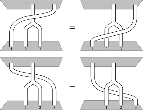
Figure 1: Compatibility of fusion and braiding as expressed by the quasitriangularity conditions. It makes no difference whether a third particle braids with two particles separately or with the composite that arises after fusing these two particles. The ribbons represent the trajectories of the particles.

Relation (3.7) implies that the comultiplication (5.4), the associator (5.14) and the braid operator (5.15) satisfy the so-called quasitriangularity conditions:

$${\cal R}\>\Delta(\,{\mbox{P}}_{A}\,B\,) = \Delta(\,{\mbox{P}}_{A}\,B\,)\>{\cal R}$$ (5.17)

$$({\mbox{id}}\otimes\Delta)({\cal R}) = \Phi^{-1}\;{\cal R}_{2}\;\Phi\;{\cal R}_{1}\;\Phi^{-1}$$ (5.18)

$$(\Delta\otimes{\mbox{id}})({\cal R}) = \Phi\;{\cal R}_{1}\;\Phi^{-1}\;{\cal R}_{2}\;\Phi\,.$$ (5.19)

Here, the braid operator ${\cal R}_{1}$ acts as ${\cal R}\otimes{\mbox{\bf 1}}$ on the three particle internal Hilbert space $(V_{\alpha}^{A}\otimes V_{\beta}^{B})\otimes V_{\gamma}^{C}$ and ${\cal R}_{2}$ as ${\mbox{\bf 1}}\otimes{\cal R}$ on $V_{\alpha}^{A}\otimes(V_{\beta}^{B}\otimes V_{\gamma}^{C})$. The condition (5.17) obviously states that the action of $D^{\omega}(H)$ on a two-particle internal Hilbert space commutes with the braid operation. The conditions (5.18) and (5.19), in turn, indicate that the following hexagonal diagrams commute

$$\begin{array}[]{ccccc}V^{A}_{\alpha}\otimes(V^{B}_{\beta}\otimes V^{C}_{\gamma})&\stackrel{{\scriptstyle\Phi^{-1}}}{{\rightarrow}}&(V^{A}_{\alpha}\otimes V^{B}_{\beta})\otimes V^{C}_{\gamma}&\stackrel{{\scriptstyle{\cal R}_{1}}}{{\rightarrow}}&(V^{B}_{\beta}\otimes V^{A}_{\alpha})\otimes V^{C}_{\gamma}\\ \downarrow{\scriptstyle({\mbox{\scriptsize id}}\otimes\Delta)({\cal R})}&&&&\downarrow{\scriptstyle\Phi}\\ (V^{B}_{\beta}\otimes V^{C}_{\gamma})\otimes V^{A}_{\alpha}&\stackrel{{\scriptstyle\Phi^{-1}}}{{\leftarrow}}&V^{B}_{\beta}\otimes(V^{C}_{\gamma}\otimes V^{A}_{\alpha})&\stackrel{{\scriptstyle{\cal R}_{2}}}{{\leftarrow}}&V^{B}_{\beta}\otimes(V^{A}_{\alpha}\otimes V^{C}_{\gamma})\\ &&&&\\ (V^{A}_{\alpha}\otimes V^{B}_{\beta})\otimes V^{C}_{\gamma}&\stackrel{{\scriptstyle\Phi}}{{\rightarrow}}&V^{A}_{\alpha}\otimes(V^{B}_{\beta}\otimes V^{C}_{\gamma})&\stackrel{{\scriptstyle{\cal R}_{2}}}{{\rightarrow}}&V^{A}_{\alpha}\otimes(V^{C}_{\gamma}\otimes V^{B}_{\beta})\\ \downarrow{\scriptstyle(\Delta\otimes{\mbox{\scriptsize id}})({\cal R})}&&&&\downarrow{\scriptstyle\Phi^{-1}}\\ V^{C}_{\gamma}\otimes(V^{A}_{\alpha}\otimes V^{B}_{\beta})&\stackrel{{\scriptstyle\Phi}}{{\leftarrow}}&(V^{C}_{\gamma}\otimes V^{A}_{\alpha})\otimes V^{B}_{\beta}&\stackrel{{\scriptstyle{\cal R}_{1}}}{{\leftarrow}}&(V^{A}_{\alpha}\otimes V^{C}_{\gamma})\otimes V^{B}_{\beta}\,.\end{array}$$

In other words, these conditions express the compatibility of braiding and fusion as depicted in figure 1.

Due to the finite order of the braid operator, multi-particle systems in planar discrete gauge theories without CS action realize representations of factor groups  of the well-known braid groups [9, 35]. This property persists if one adds a CS action $\omega\in H^{3}({H},U(1))$ to an abelian discrete $H$ gauge theory (or a nonabelian one for that matter). However, from the quasitriangularity conditions (5.17)–(5.19), we infer that instead of the ordinary Yang-Baxter equation, the braid operators now satisfy the quasi-Yang-Baxter equation

$${\cal R}_{1}\;\Phi^{-1}\,{\cal R}_{2}\,\Phi\;{\cal R}_{1} = \Phi^{-1}\,{\cal R}_{2}\,\Phi\;{\cal R}_{1}\;\Phi^{-1}\,{\cal R}_{2}\,\Phi\,.$$ (5.21)

Hence, the truncated braid group representations realized by the multi-particle systems in abelian discrete CS gauge theories in principle involve the associator (5.2), which takes care of the rearrangement of brackets. Let $(((V_{\alpha_{1}}^{A_{1}}\otimes V_{\alpha_{2}}^{A_{2}})\otimes\cdots\otimes V_{\alpha_{n-1}}^{A_{n-1}})\otimes V_{\alpha_{n}}^{A_{n}})$ denote an internal Hilbert space for a system of $n$ particles. Thus, all left brackets occur at the beginning. Depending on whether we are dealing with a system of identical particles, distinguishable particles, or a system consisting of different subsystems of identical particles, the associated $n$-particle internal Hilbert space $(((V_{\alpha_{1}}^{A_{1}}\otimes V_{\alpha_{2}}^{A_{2}})\otimes\cdots\otimes V_{\alpha_{n-1}}^{A_{n-1}})\otimes V_{\alpha_{n}}^{A_{n}})$ then carries an unitary representation of an ordinary truncated braid group, a colored truncated braid group or a partially colored truncated braid group on $n$ strands respectively. This representation is defined by the formal assignment [38]

$$\tau_{i} \longmapsto \Phi_{i}^{-1}\;{\cal R}_{i}\;\Phi_{i}\,,$$ (5.22)

with $1\leq i\leq n-1$ and

$${\cal R}_{i} := {\mbox{\bf 1}}^{\otimes(i-1)}\otimes{\cal R}\otimes{\mbox{\bf 1}}^{\otimes(n-i-1)}$$ (5.23)

$$\Phi_{i} := \left(\bigotimes_{i=1}^{n}\Pi_{\alpha_{i}}^{A_{i}}\right)\left(\Delta_{L}^{i-2}(\varphi)\otimes 1^{\otimes(n-i-1)}\right)\,.$$ (5.24)

Here, $\varphi$ is the associator (5.2), whereas the object $\Delta_{L}$ stands for the mapping

$$\Delta_{L}(\,{\mbox{P}}_{C_{1}}\,D_{1}\otimes{\mbox{P}}_{C_{2}}\,D_{2}\otimes\cdots\otimes{\mbox{P}}_{C_{m}}\,D_{m}\,) := \Delta(\,{\mbox{P}}_{C_{1}}\,D_{1}\,)\otimes{\mbox{P}}_{C_{2}}\,D_{2}\otimes\cdots\otimes{\mbox{P}}_{C_{m}}\,D_{m}\,,$$

from $D^{\omega}({H})^{\otimes m}$ to $D^{\omega}({H})^{\otimes(m+1)}$ and $\Delta_{L}^{k}$ for the associated mapping from $D^{\omega}({H})^{\otimes m}$ to $D^{\omega}({H})^{\otimes(m+k)}$ being the result of applying $\Delta_{L}$ $k$ times. The isomorphism (5.24) now parenthesizes the adjacent internal Hilbert spaces $V_{\alpha_{i}}^{A_{i}}$ and $V_{\alpha_{i+1}}^{A_{i+1}}$ and ${\cal R}_{i}$ acts as (5.16) on this pair of internal Hilbert spaces. At this point, it is important to note that the 3-cocycles of type I and type II, displayed in (3.16) and (3.17), are symmetric in the two last entries, i.e. $\omega(A,B,C)=\omega(A,C,B)$. This implies that the isomorphism $\Phi_{i}$ commutes with the braid operation ${\cal R}_{i}$ for these 3-cocycles. A similar observation appears for the 3-cocycles of type III given in (3.18). To start with, $\Phi_{i}$ obviously commutes with ${\cal R}_{i}$, iff the exchanged particles carry the same fluxes, that is, $A_{i}=A_{i+1}$. Since the 3-cocycles of type III are not symmetric in their last two entries, this no longer holds when the particles carry different fluxes $A_{i}\neq A_{i+1}$. In this case, however, only the monodromy operation ${\cal R}_{i}^{2}$ is relevant, which clearly commutes with the isomorphism $\Phi_{i}$. The conclusion is that the isomorphism $\Phi_{i}$ drops out of the formal definition (5.22) of the truncated braid group representations in CS theories with an abelian finite gauge group $H$. It should be stressed, though, that this simplification only occurs for abelian gauge groups $H$. In CS theories with a nonabelian finite gauge group, in which the fluxes exhibit flux metamorphosis [11], the isomorphism $\Phi_{i}$ has to be taken into account [35].

All in all, the internal Hilbert space of a multi-particle system in an abelian discrete gauge theory with CS action $\omega\in H^{3}({H},U(1))$ carries a representation of he quasi-quantum double $D^{\omega}(H)$ and some truncated braid group. Both representations are in general reducible. It is now easily verified that relation (5.17) extends to an internal Hilbert space describing an arbitrary number of particles and states that the action of the quasi-quantum double commutes with the action of the related truncated braid group. Hence, the multi-particle internal Hilbert space in these theories, in fact, decomposes into irreducible subspaces under the action of the direct product of $D^{\omega}(H)$ and the related truncated braid group. I will discuss this decomposition and the relation with the spins assigned to the particles in further detail in the following subsection.

As a last remark, it can be shown [16] that the deformation of the quantum double $D(H)$ into the quasi-quantum double $D^{\omega}(H)$ just depends on the cohomology class of $\omega$ in $H^{3}(H,U(1)$. That is, the quasi-quantum double $D^{\omega\delta\beta}({H})$ with $\delta\beta$ a 3-coboundary is isomorphic to $D^{\omega}({H})$, which is consistent with the fact (see section 3.2) that these 3-cocycles define equivalent CS theories.

5.2 Fusion, spin and braid statistics

Let $(\Pi^{A}_{\alpha},V_{\alpha}^{A})$ and $(\Pi^{B}_{\beta},V_{\beta}^{B})$ be two irreducible representations of $D^{\omega}(H)$ defined in (5.8). The tensor product representation $(\Pi^{A}_{\alpha}\otimes\Pi^{B}_{\beta},V_{\alpha}^{A}\otimes V_{\beta}^{B})$ constructed by means of the comultiplication (5.4) in general decomposes into a direct sum of irreducible representations

$$\Pi^{A}_{\alpha}\otimes\Pi^{B}_{\beta} = \bigoplus_{C,\gamma}N^{AB\gamma}_{\alpha\beta C}\;\Pi^{C}_{\gamma}\,,$$ (5.25)

with $N^{AB\gamma}_{\alpha\beta C}$ the multiplicity of the irreducible representation $(\Pi^{C}_{\gamma},V^{C}_{\gamma})$ given by [16]

$$N^{AB\gamma}_{\alpha\beta C} = \frac{1}{|{H}|}\,\sum_{D,E}\mbox{tr}\left(\Pi^{A}_{\alpha}\otimes\Pi^{B}_{\beta}(\Delta(\,{\mbox{P}}_{E}\,D\,))\right)\;\mbox{tr}\left(\Pi^{C}_{\gamma}(\,{\mbox{P}}_{E}\,D\,)\right)^{*}$$

$$= \delta_{C,A\cdot B}\;\frac{1}{|{H}|}\,\sum_{D}\mbox{tr}\left(\alpha(D)\right)\;\mbox{tr}\left(\beta(D)\right)\;\mbox{tr}\left(\gamma(D)\right)^{*}\;c_{D}(A,B)\,.$$

Here, tr stands for taking the trace, $|{H}|$ for the order of the abelian group ${H}$, $*$ for complex conjugation and $c_{D}(A,B)$ for the 2-cocycle (3.7). The so-called fusion rule (5.25) determines which particles $(\,C,\gamma\,)$ can be formed in the composition of two given particles $(\,A,\alpha\,)$ and $(\,B,\beta\,)$, or if read backwards, gives the decay channels of the particle $(\,C,\gamma\,)$. The Kronecker delta in (5.2) then indicates that the various composites $(\,C,\gamma\,)$ which may result from fusing the particles $(\,A,\alpha\,)$ and $(\,B,\beta\,)$ carry the flux $C=A\cdot B$, whereas the rest of the formula determines the composition rules for the dyon charges $\alpha$ and $\beta$.

The fusion algebra spanned by the elements $\Pi^{A}_{\alpha}$ with multiplication rule (5.25) is commutative and associative and can therefore be diagonalized. The matrix implementing this diagonalization is the so-called modular $S$ matrix [39]

$$S^{AB}_{\alpha\beta} = \frac{1}{|{H}|}\,\mbox{tr}\;{\cal R}^{-2\;AB}_{\;\;\;\;\;\alpha\beta}\;=\;\frac{1}{|{H}|}\,\mbox{tr}\left(\alpha(B)\right)^{*}\;\mbox{tr}\left(\beta(A)\right)^{*}\,.$$ (5.27)

This matrix contains all information concerning the fusion algebra (5.25). In particular, the multiplicities (5.2) can be expressed in terms of the modular $S$ matrix by means of Verlinde’s formula [39]

$$N^{AB\gamma}_{\alpha\beta C} = \sum_{D,\delta}\frac{S^{AD}_{\alpha\delta}S^{BD}_{\beta\delta}(S^{*})^{CD}_{\gamma\delta}}{S^{eD}_{0\delta}}\,.$$ (5.28)

Whereas the modular $S$ matrix is determined through the monodromy operator following from (5.16), the modular matrix $T$ contains the spin factors (5.13) assigned to the particles in the spectrum of an abelian discrete $H$ CS theory

$$T^{AB}_{\alpha\beta} = \delta_{\alpha,\beta}\,\delta^{A,B}\;\exp(2\pi\imath s_{(A,\alpha)})\;=\;\delta_{\alpha,\beta}\,\delta^{A,B}\frac{1}{d_{\alpha}}\,\mbox{tr}\left(\alpha(A)\right)\,,$$ (5.29)

with $d_{\alpha}$ the dimension of the projective dyon charge representation $\alpha$. The matrices (5.27) and (5.29) now realize an unitary representation of the discrete modular group $SL(2,{\mbox{\bf Z}})$ with the following relations [36]

$$\halign to=0.0pt{\hskip\@centering$\displaystyle{#}$\@eqnsel&\global\@eqcnt\@ne\hskip\tw@\arraycolsep\hfil${#}$\hfil&\global\@eqcnt\tw@\hskip\tw@\arraycolsep$\displaystyle{#}$\hfil&\global\@eqcnt\thr@@\hskip\tw@\arraycolsep\hfil\hbox{#}&\global\@eqcnt 4 \hbox\bgroup\hss#\egroup\cr 0.0pt plus 1000.0pt$\displaystyle{{\cal C} &10.0pt\hfil${=&10.0pt$\displaystyle{(ST)^{3} \; = \; S^{2}\, , &10.0pt\hfil\hbox{ \\ S^* &{\hss=}&{\cal C}S\;=\;S^{-1}\,,&$\qquad S^t \;=\; S \, , $\\T^{*}&=&T^{-1}\,,&$\qquad T^t \;=\; T \, ,$(5.30)\cr}}}}}$$

The relations (5.2) and (5.2) express the fact that the matrices (5.27) and (5.29) are symmetric and unitary. To proceed, the matrix ${\cal C}$ defined in (5.2) represents the charge conjugation operator which assigns an unique anti-partner ${\cal C}\,(\,A,\alpha\,)=(\,\bar{A},\bar{\alpha}\,)$ to every particle $(\,A,\alpha\,)$ in the spectrum such that the vacuum channel occurs in the fusion rule (5.25) for the particle/anti-particle pairs. Also note that the complete set of relations (5.2)–(5.2) indicate that the charge conjugation matrix ${\cal C}$ commutes with the modular matrix $T$, which implies that a given particle carries the same spin as its anti-partner.

We are now well prepared to address the issue of braid statistics and the fate of the spin-statistics connection in these 2+1 dimensional models. Let me emphasize from the outset that much of what follows has been established elsewhere in a more general setting. See for instance [34, 40] and the references therein for the 1+1 dimensional conformal field theory point of view and [2, 41] for the related 2+1 dimensional space time perspective.

We first focus on a system consisting of two distinguishable particles $(\,A,\alpha\,)$ and $(\,B,\beta\,)$. The associated two particle internal Hilbert space $V_{\alpha}^{A}\otimes V_{\beta}^{B}$ carries a representation of the cyclic truncated colored braid group $P(2,m)\simeq{\mbox{\bf Z}}_{m/2}$ (defined in appendix B) with $m/2\in{\mbox{\bf Z}}$ the order of the monodromy matrix ${\cal R}^{2}$ depending on the nature of the two particles. The aforementioned representation decomposes into a direct sum of one dimensional irreducible subspaces, each being labeled by the associated eigenvalue of the monodromy matrix ${\cal R}^{2}$. As follows immediately from relation (5.17), the monodromy operation commutes with the action of the quasi-quantum double. This implies that the decomposition (5.25) simultaneously diagonalizes the monodromy matrix. That is, the two particle total flux/charge eigenstates spanning a given fusion channel $V_{\gamma}^{C}$ all carry the same monodromy eigenvalue, which in addition can be shown to satisfy the generalized spin-statistics connection [16]

$$K^{ABC}_{\alpha\beta\gamma}\;{\cal R}^{2} = e^{2\pi\imath(s_{(C,\gamma)}-s_{(A,\alpha)}-s_{(B,\beta)})}\;\;K^{ABC}_{\alpha\beta\gamma}\,.$$ (5.31)

Here, $K^{ABC}_{\alpha\beta\gamma}$ stands for the projection on the irreducible component $V_{\gamma}^{C}$ of $V_{\alpha}^{A}\otimes V_{\beta}^{B}$. So, the monodromy operation on a two particle state in a given fusion channel is the same as a clockwise rotation over an angle of $2\pi$ of the two particles separately accompanied by a counterclockwise rotation over an angle of $2\pi$ of the single particle state emerging after fusion. This is consistent with the fact that these two processes can be continuously deformed into each other, which is easily verified with the associated ribbon diagrams depicted in figure 2. The discussion can now be summarized by the statement that the total internal Hilbert space $V_{\alpha}^{A}\otimes V_{\beta}^{B}$ decomposes into the following direct sum of irreducible representations of the direct product $D^{\omega}(H)\times P(2,m)$

$$\bigoplus_{C,\gamma}N^{AB\gamma}_{\alpha\beta C}\;(\Pi^{C}_{\gamma},\Lambda_{C-A-B})\,,$$ (5.32)

where $\Lambda_{C-A-B}$ denotes the one dimensional irreducible representation of $P(2,m)$ in which the generator $\gamma_{12}$ of $P(2,m)$ acts as (5.31).

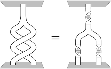
Figure 2: Generalized spin-statistics connection. The displayed ribbon diagrams are homotopic as can be checked with a pair of pants. In other words, a monodromy of two particles in a given fusion channel followed by fusion of the pair can be continuously deformed into the process describing a rotation over an angle of $-2\pi$ of the two particles seperately followed by fusion of the pair and a final rotation over an angle of $2\pi$ of the composite.

The discussion for a system of two identical particles $(\,A,\alpha\,)$ is similar. The total internal Hilbert space $V_{\alpha}^{A}\otimes V_{\alpha}^{A}$ now decomposes into one dimensional irreducible subspaces under the action of the cyclic truncated braid group $B(2,m)\simeq{\mbox{\bf Z}}_{m}$. In the conventions set in appendix B, $m$ denotes the order of the braid operator ${\cal R}$, which depends on the system under consideration. By the same argument as before, the two particle total flux/charge eigenstates spanning a given fusion channel $V_{\gamma}^{C}$ all carry the same one dimensional representation of $B(2,m)$. The quantum statistics phase assigned to this channel now satisfies the square root version of the generalized spin-statistics connection (5.31)

$$K^{AAC}_{\alpha\alpha\gamma}\;{\cal R} = \epsilon\;e^{\pi\imath(s_{(C,\gamma)}-2s_{(A,\alpha)})}\;\;K^{AAC}_{\alpha\alpha\gamma}\,,$$ (5.33)

with $\epsilon$ a sign depending on whether the fusion channel $V_{\gamma}^{C}$ appears in a symmetric or an anti-symmetric fashion [34]. Thus, the internal space Hilbert space for a system of two identical particles $(\,A,\alpha\,)$ breaks up into the following irreducible representations of the direct product $D^{\omega}(H)\times B(2,m)$

$$\bigoplus_{C,\gamma}N^{AA\gamma}_{\alpha\alpha C}\;(\Pi^{C}_{\gamma},\Lambda_{C-2A})\,,$$ (5.34)

with $\Lambda_{C-2A}$ the one dimensional representation of the truncated braid group $B(2,m)$ defined in (5.33).

In fact, the generalized spin-statistics connection (5.33) incorporates the so-called canonical one. This can be seen using a topological proof of the canonical spin-statistics connection orginally due to Finkelstein and Rubinstein [42]. Finkelstein and Rubinstein restricted themselves to skyrmions in 3+1 dimensions, but their argument naturally extends to particles in 2+1 dimensional space time. (See also reference [43] and [41] for an algebraic approach.) The crucial ingredient in their topological proof of the canonical spin-statistics connection for a given model is the existence of an anti-particle for every particle in the spectrum such that the pair can annihilate into the vacuum after fusion. Given this, one may then consider the process depicted at the l.h.s. of the equality sign in figure 3. It describes the creation of two separate identical particle/anti-particle pairs from the vacuum, a subsequent counterclockwise exchange of the particles of the two pairs and a final annihilation of the two pairs. It is readily checked that the closed ribbon associated with the process just explained can be continuously deformed into the ribbon at the r.h.s. of figure 3 corresponding to a counterclockwise rotation of the particle over an angle of $2\pi$ around its own centre. In other words, the effect of interchanging two identical particles in a consistent quantum description should be the same as the effect of rotating one particle over an angle of $2\pi$ around its centre. The effect of this rotation in the wave function is the spin factor $\exp(2\pi\imath s)$ with $s$ the spin of the particle (which may take any real value in 2+1 dimensional space time). Therefore, the result of exchanging the two identical particles necessarily boils down to a quantum statistical phase factor $\exp(\imath\Theta)$ in the wave function being the same as the spin factor

$$\exp(\imath\Theta) = \exp(2\pi\imath s)\,.$$ (5.35)

This relation is known as the canonical spin-statistics connection. Actually, a further consistency condition can be inferred from this ribbon argument. The writhing in the particle trajectory can be continuously deformed into a writhing with the same orientation in the anti-particle trajectory. Hence, the anti-particle necessarily carries the same spin and statistics as the particle.

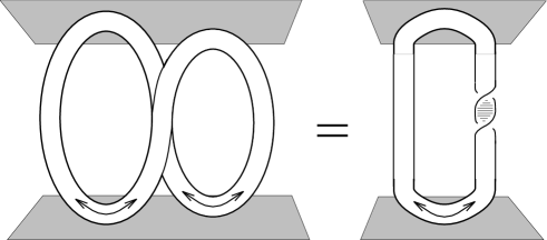
Figure 3: Canonical spin-statistics connection. The particle trajectories describing a counterclockwise interchange of two particles in separate particle/anti-particle pairs (the 8 laying on its back) can be continuously deformed into a single pair in which the particle undergoes a counterclockwise rotation over an angle of $2\pi$ around its own centre (the 0 with a twisted leg).

The basic assertions for the foregoing topological proof of the canonical spin-statistics connection are satisfied in the abelian discrete $H$ CS theories under consideration. That is to say, for every particle $(\,A,\alpha\,)$ in the spectrum there exists an anti-particle $(\,{\bar{A}},\bar{\alpha}\,)$ such that under the proper composition the pair acquires the quantum numbers of the vacuum and may decay. Moreover, as indicated by the fact that the charge conjugation operator ${\cal C}$ commutes with the modular matrix $T$, every particle carries the same spin as its anti-partner. It should be noted now that the ribbon argument in figure 3 actually only applies to states in which the particles that propagate along the exchanged ribbons are in strictly identical internal states. Otherwise the ribbons can not be closed. Indeed, we find that the action (5.16) of the braid operator on two particles in identical internal flux/charge eigenstates

$${\cal R}\;|\,A,\,^{\alpha}\!v_{j}\rangle|\,A,\,^{\alpha}\!v_{j}\rangle = |\,A,\,\alpha\,(\,^{A}\!h_{1}\,)_{mj}\,^{\alpha}\!v_{m}\rangle|\,A,\,^{\alpha}\!v_{j}\rangle\,,$$ (5.36)

boils down to the diagonal matrix (5.13) and therefore to the same spin factor (5.37)

$$\exp(\imath\Theta_{(A,\alpha)}) = \exp(2\pi\imath s_{(A,\alpha)})\,,$$ (5.37)

for all $j$. The conclusion is that the canonical spin-statistics connection holds in the fusion channels spanned by linear combinations of the states (5.36) in which the particles are in strictly identical internal flux/charge eigenstates. The quantum statistics phase (5.33) assigned to these channels reduces to the spin factor in (5.37). Thus the effect of a counterclockwise interchange of the two particles in the states in these channels is the same as the effect of rotating one of the particles over an angle of $2\pi$. To conclude, the closed ribbon proof does not apply to the other channels and we are left with the more involved connection (5.33) following from the open ribbon argument displayed in figure 2.

Higher dimensional irreducible truncated braid group representations are conceivable for systems consisting of more than two particles in abelian discrete $H$ gauge theories with a type III CS action (3.18). The occurrence of such representations simply means that the generators of the associated truncated braid group can not be diagonalized simultaneously. What happens in this situation is that under the full set of braid operations, the system jumps between isotypical fusion channels, i.e. fusion channels of the same type or ‘color’. Let us make this statement more precise. To keep the discussion general, we do not specify the nature of the particles in the system. Depending on whether the system consists of identical particles, distinguishable particles or some ‘mixture’, we are dealing with a truncated braid group, a colored truncated braid group or a partially colored truncated braid group respectively. The decomposition of the internal Hilbert for a system of more then two particles into a direct sum of irreducible subspaces (or fusion channels) under the action of the quasi-quantum double $D^{\omega}(H)$ simply follow from the fusion rules (5.25) and the fact that the fusion algebra is associative. Given that the action of the associated truncated braid group commutes with that of the quasi-quantum double, we are left with two possibilities. On the one hand, there will in general be some fusion channels being separately invariant under the action of the associated truncated braid group. As in the two particle systems discussed before, the total flux/charge eigenstates spanning such a fusion channel, say $V_{\gamma}^{C}$, carry the same one dimensional irreducible representation $\Lambda_{\mbox{\scriptsize abelian}}$ of the related truncated braid group. That is, these states realize abelian braid statistics with the same quantum statistics or monodromy phase. So, the fusion channel $V_{\gamma}^{C}$ carries the irreducible representation $(\Pi_{\gamma}^{C},\Lambda_{\mbox{\scriptsize abelian}})$ of the direct product of the quasi-quantum double and the related truncated braid group. On the other hand, it is also feasible that states carrying the same total flux and charge in different (isotypical) fusion channels are mixed under the action of the related truncated braid group. In that case, we are dealing with a higher dimensional irreducible representation of the truncated braid group or nonabelian braid statistics. Note that nonabelian braid statistics is conceivable, if and only if some fusion channel, say $V_{\delta}^{D}$, occurs more then once in the decomposition of the Hilbert space under the action of $D^{\omega}(H)$. Only then there are some orthogonal states with the same total flux and charge available to span an higher dimensional irreducible representation of the associated truncated braid group. The number $n$ of fusion channels $V_{\delta}^{D}$ related by the action of the braid operators now constitutes the dimension of the irreducible representation $\Lambda_{\mbox{\scriptsize nonabelian}}$ of the braid group and the multiplicity of this representation is the dimension $d$ of the fusion channel $V_{\delta}^{D}$. To conclude, the direct sum of these $n$ fusion channels $V_{\delta}^{D}$ then carries an $n\cdot d$ dimensional irreducible representation $(\Pi_{\delta}^{D},\Lambda_{\mbox{\scriptsize nonabelian}})$ of the direct product of $D^{\omega}(H)$ and the associated truncated braid group.

6 $U(1)$ Chern-Simons theory

We turn to the simplest example of a spontaneously broken CS gauge theory, namely the planar abelian Higgs model equipped with a CS term (4.2) for the gauge fields. So, the action of the model under consideration reads

$$S = \int d\,^{3}x\;({\cal L}_{\mbox{\scriptsize YMH}}+{\cal L}_{\mbox{\scriptsize matter}}+{\cal L}_{\mbox{\scriptsize CSI}})$$ (6.1)

$${\cal L}_{\mbox{\scriptsize YMH}} = -\frac{1}{4}F^{\kappa\nu}F_{\kappa\nu}+({\cal D}^{\kappa}\Phi)^{*}{\cal D}_{\kappa}\Phi-V(|\Phi|)$$ (6.2)

$${\cal L}_{\mbox{\scriptsize matter}} = -j^{\kappa}A_{\kappa}$$ (6.3)

$${\cal L}_{\mbox{\scriptsize CSI}} = \frac{\mu}{2}\epsilon^{\kappa\nu\tau}A_{\kappa}\partial_{\nu}A_{\tau}\,,$$ (6.4)

where the Higgs field $\Phi$ is assumed to carry the global $U(1)$ charge $Ne$. In our conventions, this means that the covariant derivative takes the form ${\cal D}_{\kappa}\Phi=(\partial_{\kappa}+\imath NeA_{\kappa})\Phi$. Further, the Higgs potential

$$V(|\Phi|) = \frac{\lambda}{4}(|\Phi|^{2}-v^{2})^{2}\qquad\qquad\mbox{with $\lambda,v>0\,,$}$$ (6.5)

endows the Higgs field $\Phi$ with a nonvanishing vacuum expectation value $|\langle\Phi\rangle|=v$. So, the compact $U(1)$ gauge symmetry is spontaneously broken to the finite cyclic subgroup ${\mbox{\bf Z}}_{N}$ at the energy scale $M_{H}=v\sqrt{2\lambda}$. Finally, the matter charges $q$ introduced by the current $j^{\kappa}$ in (6.3) are assumed to be multiples of the fundamental charge unit $e$. That is, $q=ne$ with $n\in{\mbox{\bf Z}}$.

In fact, with the incorporation of the topological CS term (6.4), the complete phase diagram for a compact planar $U(1)$ gauge theory endowed with matter exhibits the following structure. Depending on the parameters in our model (6.1) and the presence of Dirac monopoles/instantons, we can distinguish the phases:

• $\mu=v=0$ $\Rightarrow$ Coulomb phase. The spectrum consists of the quantized matter charges $q=ne$ exhibitting Coulomb interactions, where the Coulomb potential depends logarithmically on the distances between the charges in this two spatial dimensional setting.

• $\mu=v=0$ with Dirac monopoles $\Rightarrow$ confining phase. As has been shown by Polyakov [26], the contribution of monopoles/instantons to the partition function leads to linear confinement of the quantized charges $q$.

• $v\neq 0,\,\mu=0$ $\Rightarrow$ ${\mbox{\bf Z}}_{N}$ Higgs phase, e.g. [9, 15] and references therein. The spectrum consists of screened matter charges $q=ne$, magnetic fluxes quantized as $\phi=\frac{2\pi a}{Ne}$ with $a\in{\mbox{\bf Z}}$ and dyonic combinations. The long range interactions are topological AB interactions: in the process of circumnavigating a flux $\phi$ counterclockwise with a matter charge $q$, for instance, the wave function of the system picks up the AB phase $\exp(\imath q\phi)$. Under these remaining long range interactions, the charges and fluxes become ${\mbox{\bf Z}}_{N}$ quantum numbers. Further, in the presence of Dirac monopoles/instantons, magnetic flux $a$ is conserved modulo $N$.

• $v=0,\,\mu\neq 0$ $\Rightarrow$ CS electrodynamics [1]. The gauge fields carry the topological mass $|\mu|$. The charges $q=ne$ constituting the spectrum are screened by induced magnetic fluxes $\phi=-q/\mu$. The long range interactions between the matter charges are AB interactions with coupling constant $\sim 1/\mu$, i.e. a counterclockwise monodromy involving a charge $q$ and a charge $q^{\prime}$ gives rise [22] to the AB phase $\exp(-\imath qq^{\prime}/\mu)$. It has been argued [25, 27, 28] that the presence of Dirac monopoles does not lead to confinement of the matter charges in this massive CS phase. A consistent implementation of Dirac monopoles requires that the topological mass is quantized [25] as $\frac{pe^{2}}{\pi}$ with $p\in{\mbox{\bf Z}}$. The Dirac monopoles then describe tunneling events between particles with charge difference $\Delta q=2pe$ with $p$ the integral CS parameter. Thus, the spectrum only contains a total number of $2p-1$ distinct stable charges in this case.

• $v\neq 0,\,\mu\neq 0$ $\Rightarrow$ ${\mbox{\bf Z}}_{N}$ CS Higgs phase [14, 18, 19, 35]. Again, the spectrum features screened matter charges $q=ne$, magnetic fluxes quantized as $\phi=\frac{2\pi a}{Ne}$ with $a\in{\mbox{\bf Z}}$ and dyonic combinations. In this phase, we have the conventional long range AB interaction $\exp(\imath q\phi)$ between charges and fluxes, and, in addition, AB interactions $\exp(\imath\mu\phi\phi^{\prime})$ between the fluxes themselves [14, 18]. Under these interactions, the charges then obviously remain ${\mbox{\bf Z}}_{N}$ quantum numbers, whereas a compactification of the magnetic flux quantum numbers only occurs for fractional values of the topological mass $\mu$ [18]. In particular, the aforementioned quantization of the topological mass required in the presence of Dirac monopoles renders the magnetic fluxes to be ${\mbox{\bf Z}}_{N}$ quantum numbers. The flux tunneling $\Delta a=-N$ induced by the minimal Dirac monopole is now accompanied by a charge jump $\Delta n=2p$, with $p$ the integral CS parameter. Finally, as implied by the homomorphism (4.8) for this case, the CS parameter becomes periodic in this broken phase, that is, there are just $N-1$ distinct ${\mbox{\bf Z}}_{N}$ CS Higgs phases in which both charges and fluxes are ${\mbox{\bf Z}}_{N}$ quantum numbers [18, 19].

In this section, we just focus on the phases summarized in the last two items. The discussion is organized as follows. Subsection 6.1 contains a brief exposition of CS electrodynamics featuring Dirac monopoles. In subsection 6.2, we then turn to the CS Higgs screening mechanism for the electromagnetic fields generated by the matter charges and the magnetic vortices in the broken phase and establish the above mentioned long range AB interactions between these particles. To conclude, a detailed discussion of the discrete ${\mbox{\bf Z}}_{N}$ CS gauge theory describing the long distance physics in the broken phase is presented in subsection 6.3.

6.1 Dirac monopoles and topological mass quantization

For future use and reference, I begin by briefly reviewing the basic features of CS electrodynamics, i.e. we set the symmetry breaking scale in our model (6.1) to zero for the moment ($v=0$) and take $\mu\neq 0$. Varying the action (6.1) w.r.t. the vector potential $A_{\kappa}$ then yields the field equations

$$\partial_{\nu}F^{\nu\kappa}+\mu\epsilon^{\kappa\nu\tau}\partial_{\nu}A_{\tau} = j^{\kappa}+j^{\kappa}_{H}\,,$$ (6.6)

where

$$j^{\kappa}_{H} = \imath Ne(\Phi^{*}{\cal D}^{\kappa}\Phi-({\cal D}^{\kappa}\Phi)^{*}\Phi)\,,$$ (6.7)

denotes the Higgs current and $j^{\kappa}$ the matter current in (6.3). These field equations indicate that the gauge fields are massive. To be precise, this model features a single component photon carrying the topological mass $|\mu|$ [1]. So, the electromagnetic fields generated by the currents in (6.6) are screened: they fall off exponentially with mass $|\mu|$. Hence, at distances $\gg 1/|\mu|$ the Maxwell term in (6.6) can be neglected which immediately reveals how the screening mechanism operating in CS electrodynamics works. The currents $j^{\kappa}$ and $j^{\kappa}_{H}$ induce magnetic flux currents $-\frac{1}{2}\epsilon^{\kappa\nu\tau}\partial_{\nu}A_{\tau}$ exactly screening the electromagnetic fields generated by $j^{\kappa}$ and $j^{\kappa}_{H}$. Specifically, from Gauss’ law

$$Q=q+q_{H}+\mu\phi=0\,,$$ (6.8)

with $Q=\int\!d\,^{2}x\,\nabla\!\cdot\!{\mbox{\bf E}}=0$, $q=\int\!d\,^{2}x\,j^{0}$, $q_{H}=\int\!d\,^{2}x\,j^{0}_{H}$ and $\phi=\int\!d\,^{2}x\,\epsilon^{ij}\partial_{i}A^{j}$, we learn that the CS screening mechanism attaches fluxes $\phi=-q/\mu$ and $\phi_{H}=-q_{H}/\mu$ of characteristic size $1/|\mu|$ to the point charges $q$ and $q_{H}$ respectively [1].

The remaining long range interactions between these screened charges $q$ are the topological AB interactions [10] implied by the matter coupling (6.3) and the CS coupling (6.4). These can be summarized [22] as 

$${\cal R}^{2}\;|q\rangle|q^{\prime}\rangle = e^{-\imath\frac{qq^{\prime}}{\mu}}|q\rangle|q^{\prime}\rangle$$ (6.9)

$${\cal R}\;|q\rangle|q\rangle = e^{-\imath\frac{qq}{2\mu}}\,|q\rangle|q\rangle\,.$$ (6.10)

So, the particles in this theory realize abelian braid statistics. Particularly, relation (6.10) indicates that identical particle configurations in general exhibit anyon statistics [3] with quantum statistics phase $\exp(\imath\Theta_{q})=\exp(-\imath\frac{qq}{2\mu})$ depending on the square of the charge $q$ of the particles and the inverse of the topological mass $\mu$. Further, the assertions for the topological proof of the canonical spin-statistics connection (5.35) are obviously satisfied in this model. Hence, a rotation of a charge $q$ over an angle of $2\pi$ gives rise to the spin factor $\exp(2\pi\imath s_{q})=\exp(\imath\Theta_{q})=\exp(-\imath\frac{qq}{2\mu})$.

Figure 4: Spectrum of unbroken $U(1)$ CS theory. We depict the flux $\phi$ versus the global $U(1)$ charge $q$. The CS parameter $\mu$ is set to its minimal nontrivial value $\mu=\frac{e^{2}}{\pi}$, i.e. $p=1$. The arrow represents the effect of a charged Dirac monopole/instanton, which shows that there is just one stable (fermionic) particle in this theory.

Let us now assume that this compact $U(1)$ CS gauge theory features singular Dirac monopoles [23] carrying magnetic charges quantized as $g=\frac{2\pi m}{e}$ with $m\in{\mbox{\bf Z}}$. In this 2+1 dimensional model, these monopoles become instantons corresponding to tunneling events between states with flux difference and to obey Gauss’ law (6.8) also charge difference [24, 25, 27, 28]. To be explicit, the minimal Dirac monopole induces the tunneling

instanton: $$\left\{\begin{array}[]{lcl}\Delta\phi&=&-\frac{2\pi}{e}\\ \Delta q&=&\mu\frac{2\pi}{e}\,.\end{array}\right.$$ (6.13)

A consistent implementation of these Dirac monopoles requires the quantization of the matter charges $q$ in multiples of $e$ and as a direct consequence quantization of the topological mass $\mu$. Dirac’s argument [23] works also in the presence of a CS term. In this case, the argument goes as follows. The tunneling event (6.13) corresponding to the minimal Dirac monopole should be invisible to the monodromies (6.9) with the charges $q$ present in our model. In other words, the AB phase $\exp(-\imath\frac{q\Delta q}{\mu})=\exp(-\imath\frac{2\pi q}{e})$ should be trivial, which implies the charge quantization $q=ne$ with $n\in{\mbox{\bf Z}}$. Furthermore, the tunneling event (6.13) should respect this quantization rule for $q$. So, the charge jump has to be a multiple of $e$: $\Delta q=\mu\frac{2\pi}{e}=pe$ with $p\in{\mbox{\bf Z}}$, which leads to the quantization $\mu=\frac{pe^{2}}{2\pi}$. There is, however, a further restriction on the values of the topological mass $\mu$. So far, we have only considered the monodromies in this theory, but the particles connected by Dirac monopoles should as a matter of course also have the same quantum statistics phase (6.10) or equivalently the same spin factor. In particular, the spin factor for the charge $\Delta q$ connected to the vacuum $q=0$ should be trivial: $\exp(-\imath\frac{(\Delta q)^{2}}{2\mu})=\exp(-\imath\frac{\mu}{2}(\frac{2\pi}{e})^{2})=1$. The conclusion then becomes that in the presence of Dirac monopoles the topological mass is necessarily quantized as 

$$\mu = \frac{pe^{2}}{\pi}\qquad\qquad\mbox{with $p\in{\mbox{\bf Z}}$}\,,$$ (6.14)

which is the result alluded to in (4.4). To conclude the argument, substituting relation (6.14) into expression (6.13) reveals that the presence of Dirac monopoles/instantons imply that the quantized charges $q=ne$ are conserved modulo $2pe$ with $p$ being the integral CS parameter. Thus, the spectrum of this unbroken $U(1)$ CS theory just consists of $2p-1$ stable charges $q=ne$ screened by the induced magnetic fluxes $\phi=-q/\mu$. (See also [19, 28, 44] and references therein.) We have depicted this spectrum for $p=1$ in figure 4.

Alternatively, we may embed a $U(1)$ CS theory in a nonabelian compact CS gauge theory. In that case, the whole or part of the foregoing spectrum of singular Dirac monopoles turns into regular ’t Hooft-Polyakov monopoles (e.g. [9, 45, 46] and references therein). As will be illustrated next with two representative examples, the correct quantization of the topological mass is automatic. This is as it should, since the regular monopoles/instantons, in any case, can not be left out in such a theory. Let us first consider a CS theory in which the gauge group $SU(2)$ is spontaneously broken down to $U(1)$ [18, 19]. It is well-known (e.g. Deser et al. in reference [1]) that in order to end up with a gauge invariant quantum theory, the topological mass for a $SU(2)$ CS theory is necessarily quantized as $\mu_{SU(2)}=\frac{ke^{2}}{4\pi}$ with $k\in{\mbox{\bf Z}}$. At first sight, this finer quantization seems to be in conflict with (6.14). This is not the case though. The point is that the effective low energy $U(1)$ CS theory of the foregoing model features $U(1)$ matter charges quantized as $q=\frac{ne}{2}$ with $n\in{\mbox{\bf Z}}$ and regular ’t Hooft-Polyakov monopoles/instantons [9, 45, 46] with magnetic charge quantized as $g=\frac{4\pi m}{e}$ with $m\in{\mbox{\bf Z}}$. In other words, upon redefining $e\mapsto\frac{e}{2}$ the spectrum of matter and (Dirac) magnetic charges and the quantization (6.14) of the topological mass for the compact $U(1)$ CS theory discussed in the previous paragraph coincides with that for the foregoing broken theory. In short, the finer quantization of the topological mass as compared to (6.14) is perfectly consistent with the larger quantization of magnetic charge in this broken theory. For an $SO(3)$ CS gauge theory, in turn, a rather abstract argument [44] (see also [29]) showed that the integer CS parameter must be divisible by four in units in which any integer is allowed for $SU(2)$. So, $\mu_{SO(3)}=\frac{pe^{2}}{\pi}$ with $p\in{\mbox{\bf Z}}$. This is, in fact, precisely the quantization required for a consistent implementation of the ${\mbox{\bf Z}}_{2}$ Dirac monopoles [45] (carrying magnetic charge $g=\frac{2\pi m_{s}}{e}$ with $m_{s}\in 0,1$) that can be introduced in a $SO(3)$ CS theory. If this theory is subsequently broken down to $U(1)$, we obtain regular ’t Hooft-Polyakov monopoles [46] carrying magnetic charge quantized as $g=\frac{4\pi m_{r}}{e}$ with $m_{r}\in{\mbox{\bf Z}}$. Hence, with the incorporation of the aforementioned Dirac monopoles, the complete monopole spectrum in this broken theory consists of the magnetic charges $g=\frac{2\pi m}{e}$ with $m\in{\mbox{\bf Z}}$. As for the matter part, in the presence of the ${\mbox{\bf Z}}_{2}$ Dirac monopoles in the original $SO(3)$ theory, matter fields carrying faithful (i.e. half integral spin) representations of the universal covering group $SU(2)$ of $SO(3)$ are ruled out. Thus, only $U(1)$ matter charges $q$ carrying integral multiples of $e$ are conceivable in the foregoing broken theory. All in all, we then arrive at the same spectrum of matter and magnetic charges as the compact $U(1)$ CS theory of the previous paragraph, while the correct quantization of the topological mass (6.14) required for a consistent implemention of this spectrum of singular and regular monopoles is again automatic. To conclude, from the foregoing discussion it is also immediate that the natural homomorpisms (2.4) accompanying the spontaneous breakdown of these theories, i.e. the restrictions $H^{4}(BSU(2),{\mbox{\bf Z}})\rightarrow H^{4}(BU(1),{\mbox{\bf Z}})$ and $H^{4}(BSO(3),{\mbox{\bf Z}})\rightarrow H^{4}(BU(1),{\mbox{\bf Z}})$ induced by the inclusions $U(1)\subset SU(2)$ and $U(1)\subset SO(3)$ respectively, are not just onto, but even ono-to-one.

6.2 Dynamics of the Chern-Simons Higgs medium

We continue with an analysis of the Higgs phase of the model (6.1). So, from now on $v\neq 0$. To keep the discussion general, however, the topological mass $\mu$ may take any real value in this subsection. The incorporation of Dirac monopoles in this phase, which requires the quantization (6.14) of $\mu$, will be discussed in the next subsection.

Let me first recall some of the basic dynamical features of this model. To start with, the complex Higgs field $\Phi(x)=\rho(x)\exp(\imath\sigma(x))$ describes two physical degrees of freedom: the charged Goldstone boson field $\sigma(x)$ and the physical field $\rho(x)-v$ with mass $M_{H}=v\sqrt{2\lambda}$ corresponding to the charged neutral Higgs particles. The Higgs mass $M_{H}$ sets the characteristic energy scale of this model. At energies larger then $M_{H}$, the massive Higgs particles can be excited. At energies smaller then $M_{H}$ on the other hand, the massive Higgs particles are frozen in. For simplicity we will restrict ourselves to the latter low energy regime. In this case, the Higgs field is completely condensed, i.e. it acquires ground state values everywhere: $\Phi(x)\mapsto\langle\Phi(x)\rangle=v\exp(\imath\sigma(x))$. The condensation of the Higgs field implies that the Yang-Mills Higgs part (6.2) of the action reduces to

$${\cal L}_{\mbox{\scriptsize YMH}} \longmapsto -\frac{1}{4}F^{\kappa\nu}F_{\kappa\nu}+\frac{M_{A}^{2}}{2}\tilde{A}^{\kappa}\tilde{A}_{\kappa}\,,$$ (6.15)

with $\tilde{A}_{\kappa}:=A_{\kappa}+\frac{1}{Ne}\partial_{\kappa}\sigma$ and $M_{A}:=Nev\sqrt{2}.$ Hence, in the low energy regime, our model is governed by the effective action obtained from substituting (6.15) in (6.1). The effective field equations which follow from varying the resulting effective action w.r.t.  $A_{\kappa}$ and the Goldstone boson $\sigma$, respectively, read

$$\partial_{\nu}F^{\nu\kappa}+\mu\epsilon^{\kappa\nu\tau}\partial_{\nu}A_{\tau} = j^{\kappa}+j^{\kappa}_{\mbox{\scriptsize scr}}$$ (6.16)

$$\partial_{\kappa}j^{\kappa}_{\mbox{\scriptsize scr}} = 0\,.$$ (6.17)

The important difference with the field equations (6.6) for the unbroken case is that the Higgs current (6.7) has become the screening current [14]

$$j^{\kappa}_{\mbox{\scriptsize scr}} = -M_{A}^{2}\tilde{A}^{\kappa}\,.$$ (6.18)

From the equations (6.16) and (6.17), it is then readily inferred that the two polarizations $+$ and $-$ of the photon field $\tilde{A}_{\kappa}$ in the CS Higgs medium carry the masses [47]

$$M_{\pm} = \sqrt{M_{A}^{2}+\frac{1}{2}\mu^{2}\pm\frac{1}{2}\mu^{2}\sqrt{\frac{4M_{A}^{2}}{\mu^{2}}+1}}\,,$$ (6.19)

which differ by the topological mass $|\mu|$. As an aside, by setting $\mu=0$ in (6.19), we restore the fact that in the ordinary Higgs phase both polarizations of the photon carry the same mass $M_{+}=M_{-}=M_{A}$. Taking the limit $v\rightarrow 0$, on the other hand, yields $M_{+}=|\mu|$ and $M_{-}=0$. The $-$ component then ceases to be a physical degree of freedom [47] and we recover the fact that unbroken CS electrodynamics features a single component photon with mass $|\mu|$.

There are now two dually charged types of sources for electromagnetic fields in this CS Higgs medium: the quantized point charges $q=ne$ introduced by the matter current $j^{\kappa}$ and magnetic vortices [48] corresponding to holes in the CS Higgs medium of characteristic size $\sim 1/M_{H}$ carrying quantized magnetic flux. Specifically, inside the core of a vortex (i.e. $r<1/M_{H}$ with $r$ the distance to the centre of the vortex), the Higgs field vanishes ($\Phi(r=0)=0$), while outside the core ($r>1/M_{H}$) the Higgs field makes a noncontractible winding in the vacuum manifold: $\Phi(r>1/M_{H},\theta)=v\exp\left(\imath\sigma(r>1/M_{H},\theta)\right)$. Here, $\theta$ denotes the polar angle defined w.r.t. the centre of the vortex and $\sigma$ the (multi-valued) Goldstone boson

$$\sigma(r>1/M_{H},\theta+2\pi)-\sigma(r>1/M_{H},\theta) = 2\pi a\,,$$ (6.20)

with $a\in{\mbox{\bf Z}}$ to keep the Higgs field $\Phi$ itself single valued. Demanding the vortex solution to be of minimal (finite) energy also implies that the covariant derivative of the Higgs field vanishes away from the core:

$${\cal D}_{i}\Phi(r>1/M_{H},\theta)=0 \Rightarrow \tilde{A}_{i}(r>1/M_{H},\theta)=0\,.$$ (6.21)

So, the holonomy in the Goldstone boson field is accompanied by a holonomy in the gauge fields and the magnetic flux $\phi$ trapped inside the core of the vortex is quantized as

$$\phi\;=\;\oint dl^{i}A^{i}(r>1/M_{H})\;=\;\frac{1}{Ne}\oint dl^{i}\partial_{i}\sigma(r>1/M_{H})\;=\;\frac{2\pi a}{Ne}\;\;\;\;\mbox{with $a\in{\mbox{\bf Z}}\,.$}$$ (6.22)

Both the matter charges $q=ne$ and the magnetic vortices $\phi=\frac{2\pi a}{Ne}$ enter the field equations (6.16) describing the physics outside the cores of the vortices. The matter charges enter by means of the matter current $j^{\kappa}$ and the vortices through the magnetic flux current $-\frac{1}{2}\epsilon^{\kappa\nu\tau}\partial_{\nu}A_{\tau}$. From these equations, we learn that both the matter current and the flux current generate electromagnetic fields, which are screened at large distances by an induced current $j^{\kappa}_{\mbox{\scriptsize scr}}$ in the CS Higgs medium [14]. This becomes clear from Gauss’ law for this case

$$Q=q+q_{\mbox{\scriptsize scr}}+\mu\phi=0\,,$$ (6.23)

with $q_{\mbox{\scriptsize scr}}=\int d\,^{2}x\,j^{0}_{\mbox{\scriptsize scr}}=-\int d\,^{2}x\,M_{A}^{2}\tilde{A}^{0}$, which indicates that both the matter charges $q$ and the magnetic vortices $\phi$ are surrounded by localized screening charge densities $j^{0}_{\mbox{\scriptsize scr}}$. At large distances, the contribution to the long range Coulomb fields of the induced screening charges

$$\begin{array}[]{rcl}q=ne&\Rightarrow&q_{\mbox{\scriptsize scr}}=-q\\ \phi=\frac{2\pi a}{Ne}&\Rightarrow&q_{\mbox{\scriptsize scr}}=-\mu\phi\,,\end{array}$$ (6.26)

then completely cancel those of the matter charges $q$ and the fluxes $\phi$ respectively. Here, it is of course understood that the screening charge density $j^{0}_{\mbox{\scriptsize scr}}$ accompanying a magnetic vortex is localized in a ring outside the core, since inside the core the Higgs field vanishes and the CS Higgs medium is destroyed. Let me also stress that just as in the ordinary Higgs medium [9] (i.e. no CS term) the matter charges $q$ are screened by charges $q_{\mbox{\scriptsize scr}}=-q$ provided by the Higgs condensate in this CS Higgs medium and not by attaching fluxes to them as in the case of unbroken CS electrodynamics. This is already apparent from the simple fact that the irrational ‘screening’ fluxes $\phi=-q/\mu$ would render the Higgs condensate multi-valued.

An important observation [14] concerning the induced screening charges in (6.26) is that they do not exhibit the long range AB effect [10] in the process of taking them around a remote vortex. (See also [9].) The point is that the screening charge $q_{\mbox{\scriptsize scr}}$ (attached either to a matter charge $q$ or a vortex $\phi$) not only couples to the holonomy in the gauge connection $A_{\kappa}$ around a remote vortex, but also to the holonomy (6.20) in the Goldstone boson field. This is immediate from the effective low energy action following from substituting (6.15) in (6.1). Let $j_{\mbox{\scriptsize scr}}^{\kappa}$ be the screening current (6.18) associated with some screening charge $q_{\mbox{\scriptsize scr}}$. The second term at the l.h.s. of (6.15) couples this current to the massive photon field $\tilde{A}_{\kappa}$ around the remote vortex: $j_{\mbox{\scriptsize scr}}^{\kappa}\tilde{A}_{\kappa}$. As we have seen in (6.21), outside the core of the vortex, the holonomies in the gauge fields and the Goldstone boson are related such that $\tilde{A}_{\kappa}$ strictly vanishes. Consequently, as long as the screening charge stays well away from the core of the vortex, the interaction term $j_{\mbox{\scriptsize scr}}^{\kappa}\tilde{A}_{\kappa}$ vanishes and therefore does not generate an AB phase in the process of taking a screening charge around a remote vortex. This proves our claim. An immediate conclusion is that the screening charges $q_{\mbox{\scriptsize scr}}=-q$ attached to the matter charges $q$ screen the Coulomb interactions between the matter charges, but not their AB interactions with the magnetic vortices. That is, a counterclockwise monodromy of a screened charge $q$ and a remote screened magnetic flux $\phi$ leads to the conventional AB phase

$${\cal R}^{2}\;|q\rangle|\phi\rangle = e^{\imath q\phi}\;|q\rangle|\phi\rangle\,,$$ (6.27)

as implied by the coupling (6.3). Relation (6.27) summarizes all the long range interactions for the mater charges. So, in contrast with unbroken CS electrodynamics, there are no long range AB interactions between the matter charges themselves in this broken phase. Instead, we now obtain nontrivial AB interactions among the screened magnetic fluxes

$${\cal R}^{2}\;|\phi\rangle|\phi^{\prime}\rangle = e^{\imath\mu\phi\phi^{\prime}}\;|\phi\rangle|\phi^{\prime}\rangle$$ (6.28)

$${\cal R}\;|\phi\rangle|\phi\rangle = e^{\imath\frac{\mu}{2}\phi\phi}\;|\phi\rangle|\phi\rangle\,,$$ (6.29)

entirely due to the CS coupling (6.4). From (6.29), we conclude that depending on their flux and the topological mass, identical magnetic vortices realize anyon statistics.

In retrospect, the basic characteristics of the CS Higgs screening mechanism uncovered in [14] and outlined above find their confirmation in results established in earlier studies of the static magnetic vortex solutions of the abelian CS Higgs model. In fact, the study of these so-called CS vortices was started by Paul and Khare [49], who noted that they correspond to finite energy solutions carrying both magnetic flux and electric charge. Subsequently, various authors have obtained both analytical and numerical results on these static vortex solutions. See for example [50]–[57] and the references therein. Here, I just collect the main results. In general, one takes the following ansatz for a static vortex solution of the field equations corresponding to (6.1)

$$\Phi(r,\theta)=\rho(r)\exp\left(\imath\sigma(\theta)\right)\,,\qquad A_{0}(r,\theta)=A_{0}(r)\,,\qquad A_{i}(r,\theta)=-A(r)\partial_{i}\sigma(\theta)\,,$$ (6.30)

where $r$ and $\theta$ again denote the polar coordinates and $\sigma$ the multi-valued Goldstone boson

$$\sigma(\theta+2\pi)-\sigma(\theta) = 2\pi a\,,$$ (6.31)

with $a\in{\mbox{\bf Z}}$ to render the Higgs field $\Phi$ itself single valued. Regularity of the solution imposes the following boundary conditions as $r\rightarrow 0$

$$\begin{array}[]{lll}\rho\rightarrow 0\,,&A_{0}\rightarrow{\mbox{constant}}\,,&A\rightarrow 0\,,\end{array}$$ (6.33)

whereas, for finite energy, the asymptotical behavior for $r\rightarrow\infty$ becomes

$$\begin{array}[]{lll}\rho\rightarrow v\,,&A_{0}\rightarrow 0\,,&A\rightarrow\frac{1}{Ne}\,.\end{array}$$ (6.35)

From (6.35), (6.30) and (6.31) it then follows that this solution corresponds to the quantized magnetic flux (6.22).

Since the two polarizations of the photon carry the distinct masses (6.19), it seems, at first sight, that there are two different vortex solutions corresponding to a long range exponential decay of the electromagnetic fields either with mass $M_{-}$ or with mass $M_{+}$. However, a careful analysis [51] (see also [56]) of the differential equations following from the field equations with this ansatz shows that the $M_{+}$ solution does not exist for finite $r$. Hence, we are left with the $M_{-}$ solution. To proceed, it turns out that the modulus $\rho$ of the Higgs field $\Phi$ in (6.30) grows monotonically from zero (at $r=0$) to its asymptotic ground state value (6.35) at $r=1/M_{H}$, where the profile of this growth does not change much in the full range of the parameters, e.g. [56].

An important issue is, of course, whether vortices will actually form or not, i.e. whether the superconductor we are describing is type II or I respectively. In this context, the competition between the penetration depth $1/M_{-}$ of the electromagnetic fields and the coresize $1/M_{H}$ becomes important. In ordinary superconductors ($\mu=0$), an evaluation of the free energy yields that we are dealing with a type II superconductor if $M_{H}/M_{A}=\sqrt{\lambda}/Ne\geq 1$ and a type I superconductor otherwise [58]. Since $M_{-}$ is smaller then $M_{A}$, it is expected that in the presence of a CS term the type II region is extended. A perturbative analysis for small $\mu$ shows that this is indeed the case [55]. In the following, we will always assume that our parameters are adjusted such that we are in the type II region.

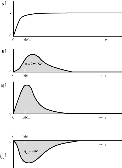
Figure 5: Qualitative behavior of the vortex solution carrying the quantized magnetic flux $\phi=\frac{2\pi a}{Ne}$ in the CS limit. We have depicted the modulus of the Higgs field $\rho$, the magnetic field $B$, the electric field $|{\mbox{\bf E}}|$ and the screening charge density $j^{0}_{\mbox{\scriptsize scr}}=-2(Ne)^{2}\rho^{2}A^{0}$, respectively, versus the radius $r$. The electromagnetic fields and the screening charge density vanish at $r=0$, reach there maximal value outside the core at $r=1/M_{H}$ and subsequently drop off exponentially with mass $M_{-}$ at larger distances.

Let us now briefly recall the structure of the electromagnetic fields of the vortex solution in the full range of parameters. To start with, the distribution of the magnetic field $B=\partial_{1}A^{2}-\partial_{2}A^{1}$ strongly depends on the topological mass $\mu$. For $\mu=0$, we are dealing with the Abrikosov-Nielsen-Olesen vortex [48]. In that case, the magnetic field reaches its maximal value at the center ($r=0$) of the vortex and drops off exponentially with mass $M_{A}$ at distances $r>1/M_{H}$. For $\mu\neq 0$, the magnetic field then decays exponentially with mass $M_{-}$ at distances $r>1/M_{H}$. Moreover, as $|\mu|$ increases from zero, the magnetic field at the origin $r=0$ diminishes until it completely vanishes in the so-called CS limit: $e,|\mu|\rightarrow\infty$, with fixed ratio $e^{2}/\mu$ [56]. (Note that in case the topological mass $\mu$ is quantized as (6.14), this limit simply means $e\rightarrow\infty$ leaving the CS parameter $p$ fixed.) Hence, in the CS limit, which amounts to neglecting the Maxwell term in (6.2), the magnetic field is localized in a ring-shaped region around the core at $r=1/M_{H}$ as depicted in figure 5 [52]–[56]. Further, as indicated by the zeroth component of the field equation (6.6), a magnetic field distribution $B$ generates an electric field distribution E iff $\mu\neq 0$. These electric fields are localized in a ring shaped region around the core at $1/M_{H}$ for all values of $\mu\neq 0$. Specifically, they vanish at $r=0$ and fall off exponentially with mass $M_{-}$ at distances $r>1/M_{H}$. We have seen in (6.26) how these electric fields induced by the magnetic field of the vortex are screened by the CS Higgs medium occurring at $r>1/M_{H}$. A screening charge density $j_{\mbox{\scriptsize scr}}^{0}$ develops in the neighborhood of the core of the vortex, which falls off exponentially with mass $M_{-}$ at $r>1/M_{H}$. In this static case, the screening charge density boils down to $j^{0}_{\mbox{\scriptsize scr}}=-M_{A}^{2}A^{0}$, i.e. the Goldstone boson does not contribute. The analytical and numerical evaluations in for example [52]–[56] show that the distribution of $A_{0}$ is indeed of the shape described above.

The spin that can be calculated for this classical CS vortex solution takes the value

$$s\;=\;\int d\,^{2}x\,\epsilon^{ij}x^{i}\,T^{0j}\;=\;\frac{\mu\phi^{2}}{4\pi}\,,$$ (6.36)

where $T^{0j}$ denotes the energy momentum tensor [52]–[56]. Note that this spin value is consistent with the quantum statistics phase $\exp(\imath\Theta)=\exp(\imath\mu\phi^{2}/2)$ in (6.29). That is, these vortices satisfy the canonical spin-statistics connection (5.35). This is actually a good point to resolve some inaccuracies in the literature. It is often stated (e.g. [52, 56]) that it is the fact that the CS vortices carry the charge (6.26) which leads to nontrivial AB interactions among these vortices. As we have argued, however, the screening charges $q_{\mbox{\scriptsize scr}}$ do not couple to the AB interactions [14] and the phases in (6.28) and (6.29) are entirely due to the CS term (6.4). In fact, erroneously assuming that the screening charges accompanying the vortices do couple to the AB interactions leads to the quantum statistics phase $\exp(-\imath\mu\phi^{2}/2)$, which is inconsistent with the spin (6.36) carried by these vortices. In this respect, we remark that the correct quantum statistics phase (6.29) for the vortices has also been derived in the dual formulation of this model [57].

To my knowledge, the nature of the static point charge solutions $j=(q\delta({\mbox{\bf x}}),0,0)$ of the field equations (6.16) have not been studied in the literature so far. An interesting question in this context is with which mass (6.19) the electromagnetic fields fall off around these matter charges. It is tempting to conjecture that this exponential decay corresponds to the mass $M_{+}$. The appealing overall picture would then become that the magnetic vortices $\phi$ excite the $-$ polarization of the massive photon in the CS Higgs medium, whereas the $+$ polarization is excited around the matter charges $q$.

6.3 ${\mbox{\bf Z}}_{N}$ Chern-Simons theory

I turn to the inclusion of Dirac monopoles in the ${\mbox{\bf Z}}_{N}$ CS Higgs phase discussed in the previous subsection. In other words, $\mu$ is quantized as (6.14) in the following. Among other things, it will be argued that with this particular quantization the ${\mbox{\bf Z}}_{N}$ CS theory describing the long distance physics in this Higgs phase corresponds to the 3-cocycle $\omega_{I}$ determined by the homomorphism (4.8) for this case [18, 19].

As we have seen in the previous subsection, the Higgs mechanism causes the identification of charge and flux occurring in unbroken CS electrodynamics to disappear. That is, the spectrum of the ${\mbox{\bf Z}}_{N}$ CS Higgs phase consists of the quantized matter charges $q=ne$, the quantized magnetic fluxes $\phi=\frac{2\pi a}{Ne}$ and dyonic combinations of the two. We will label these particles as $(a,n)$ with $a,n\in{\mbox{\bf Z}}$. Upon implementing the quantization (6.19) of the topological mass $\mu$, the AB interactions (6.27), (6.28) and (6.29) can be cast in the form

$${\cal R}^{2}\;|a,n\rangle|a^{\prime},n^{\prime}\rangle = e^{\frac{2\pi\imath}{N}(na^{\prime}+n^{\prime}a+\frac{2p}{N}aa^{\prime})}\;|a,n\rangle|a^{\prime},n^{\prime}\rangle$$ (6.37)

$${\cal R}\;|a,n\rangle|a,n\rangle = e^{\frac{2\pi\imath}{N}(na+\frac{p}{N}aa)}\;|a,n\rangle|a,n\rangle$$ (6.38)

$$T\;|a,n\rangle = e^{\frac{2\pi\imath}{N}(na+\frac{p}{N}aa)}\;|a,n\rangle\,,$$ (6.39)

where $p$ denotes the integral CS parameter. Expression (6.39) contains the spin factors assigned to the particles. Under these topological interactions, the charge label $n$ obviously becomes a ${\mbox{\bf Z}}_{N}$ quantum number, i.e. at large distances we are only able to distinguish the charges $n$ modulo $N$. Furthermore, in the presence of the Dirac monopoles/instantons (6.13) magnetic flux $a$ is conserved modulo $N$. However, the flux decay events are now accompanied by charge creation [15, 19]. To be specific, in terms of the integral flux and charge quantum numbers $a$ and $n$, the tunneling event induced by the minimal Dirac monopole can be recapitulated as

instanton: $$\left\{\begin{array}[]{lcl}a&\mapsto&a-N\\ n&\mapsto&n+2p\,.\end{array}\right.$$ (6.42)

I have depicted this effect of a Dirac monopole in the spectrum of a ${\mbox{\bf Z}}_{4}$ CS Higgs phase in figure 6. Recall from section 6.1 that the quantization (6.14) of the topological mass was such that the particles connected by monopoles were invisible to the monodromies (6.9) and carried the same spin in the unbroken phase. This feature naturally persists in this broken phase. It is readily checked that the particles connected by the monopole (6.42) can not be distinguished by the AB interactions (6.37) and give rise to the same spin factor (6.39). As a result, the spectrum of this broken phase can be presented as

$$(a,n)\qquad\qquad\qquad\mbox{with}\qquad a,n\in 0,1,\ldots,N-1\,,$$ (6.43)

where it is understood that the modulo $N$ calculus for the magnetic fluxes $a$ involves the charge jump (6.42).

Figure 6: The spectrum of a ${\mbox{\bf Z}}_{4}$ CS Higgs phase compactifies to the particles inside the dashed box. We depict the flux $\phi$ versus the matter charge $q$ and the screening charge $-q_{\mbox{\scriptsize scr}}=q+\mu\phi$ respectively. The CS parameter $\mu$ is set to its minimal nontrivial value $\mu=\frac{e^{2}}{\pi}$, that is, $p=1$. The arrows visualize the tunneling event induced by a minimal Dirac monopole.

Let us now explicitly verify that we are indeed dealing with a ${\mbox{\bf Z}}_{N}$ gauge theory with CS action (3.2), i.e.

$$\omega_{\mbox{\scriptsize I}}(a,b,c) = \exp\left(\frac{2\pi\imath p}{N^{2}}\,a(b+c-[b+c])\right)\,,$$ (6.44)

where the rectangular brackets denote modulo $N$ calculus such that the sum always lies in the range $0,1,\ldots,N-1$. First of all, the different particles (6.43) constitute the compactified spectrum on which the quasi-quantum double $D^{\omega_{I}}({\mbox{\bf Z}}_{N})$ acts. The additional AB interactions among the fluxes are then absorbed in the definition of the dyon charges.  To be specific, the dyon charge (5.9) corresponding to the flux $a$ is given by ${\alpha}(b)=\varepsilon_{a}(b)\;\Gamma^{n}(b)$ with $\varepsilon_{a}(b)$ defined in (3.21) as

$$\varepsilon_{a}(b) = \exp\left(\frac{2\pi\imath p}{N^{2}}ab\right),$$ (6.45)

and $\Gamma^{n}(b)=\exp\left(\frac{2\pi\imath}{N}nb\right)$ an UIR of ${\mbox{\bf Z}}_{N}$. The action of the braid operator (5.16) now gives rise to the AB phases presented in (6.37) and (6.38), whereas the action of the central element (5.11) yields the spin factor (6.39). Furthermore, the fusion rules for $D^{\omega_{I}}({\mbox{\bf Z}}_{N})$ following from (5.2)

$$(a,n)\times(a^{\prime},n^{\prime}) = \left([a+a^{\prime}],[n+n^{\prime}+\frac{2p}{N}(a+a^{\prime}-[a+a^{\prime}])]\right)\,,$$ (6.46)

express the tunneling properties of the Dirac monopoles. Specifically, if the sum of the fluxes $a+a^{\prime}$ exceeds $N-1$, the composite carries unstable flux and tunnels back to the range (6.43) by means of the charged monopole (6.42). Note that the charge jump induced by the monopole for CS parameter $p\neq 0$ implies that the fusion algebra now equals ${\mbox{\bf Z}}_{kN}\times{\mbox{\bf Z}}_{N/k}$ [36]. Here, we defined $k:=N/{\gcd}(p,N)$ for odd $N$ and $k:=N/{\gcd}(2p,N)$ for even $N$, where $\gcd$ stands for the greatest common divisor. In particular, for odd $N$ and $p=1$, the complete spectrum is generated by the single magnetic flux $a=1$. Finally, the charge conjugation operator ${\cal C}=S^{2}$ following from (5.27) takes the form

$${\cal C}\;(a,n) = \left([-a],[-n+\frac{2p}{N}(-a-[-a])]\right)\,.$$ (6.47)

So, as usual, under the action of the charge conjugation operator the fluxes $a$ and charges $n$ reverse sign. Subsequently, the ‘twisted’ modulo $N$ calculus for the fluxes (6.42) and the ordinary modulo $N$ calculus for the charges are applied to return to the range (6.43). Also, note that the particles and anti-particles in this theory naturally carry the same spin, i.e. the action (6.39) of the modular $T$ matrix indeed commutes with ${\cal C}$.

Having established that the U(1) CS term (6.4) gives rise to the 3-cocycle (6.44) in the residual ${\mbox{\bf Z}}_{N}$ gauge theory in the Higgs phase, I now turn to the periodicity $N$ of the CS parameter $p$ indicated by the homomorphism (4.8). This periodicity can be made explicit as follows. From the braid properties (6.37), the spin factors (6.39) and the fusion rules (6.46), we infer that setting the CS parameter to $p=N$ amounts to an automorphism $(a,n)\mapsto(a,[n+2a])$ of the spectrum (6.43) for $p=0$. In other words, for $p=N$ the theory describes the same topological interactions between the particles as for $p=0$. We just have relabeled the dyons.

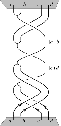
Figure 7: The 3-cocycle condition states that the topological action $\exp(\imath S_{\mbox{\scriptsize CSI}})$ for this process is trivial. The vertices in which the fluxes are fused correspond to a minimal Dirac instanton iff the total flux of the composite is larger then $N-1$.

Let me close this section by identifying the process corresponding to the CS action (6.44). A comparison of the expressions (6.44) and (6.45) yields

$$\omega_{\mbox{\scriptsize I}}(a,b,c) = \varepsilon_{b}(a)\;\varepsilon_{c}(a)\;\varepsilon^{-1}_{[b+c]}(a)\,,$$ (6.48)

from which we immediately conclude

$$\omega_{\mbox{\scriptsize I}}(a,b,c) = \exp(\imath S_{\mbox{\scriptsize CSI}})\left\{\vbox{\epsfbox{kocykle.eps}}\right\}\,.$$ (6.49)

Here, the fluxes $a$,$b$ and $c$ are again assumed to take values in the range $0,1,\ldots,N-1$. For convenience, the trajectories of the fluxes are depicted as lines rather than ribbons.  The vertex corresponding to fusion of the fluxes $b$ and $c$ then describes the tunneling event (6.42) induced by the minimal Dirac monopole iff the total flux $b+c$ of the composite exceeds $N-1$. Of course, the total AB phase for the process depicted in (6.49), which also involves the matter coupling (6.3), is trivial as witnessed by the fact that the quasitriangularity condition (5.18) is satisfied. The contribution (6.49) of the CS term (6.4) to this total AB phase, however, is nontrivial iff the vertex corresponds to a monopole. It only generates AB phases between magnetic fluxes and therefore only notices the flux tunneling at the vertex and not the charge creation. Specifically, in the first braiding of the process (6.49), the CS coupling generates the AB phase $\varepsilon_{b}(a)$, in the second $\varepsilon_{c}(a)$ and in the last $\varepsilon^{-1}_{[b+c]}(a)$. Hence, the total CS action for this process indeed becomes (6.48). With the prescription (6.49), factorization of the topological action, the so-called skein relation

$$\exp(\imath S_{\mbox{\scriptsize CSI}})\left\{\vbox{\epsfbox{actie.eps}}\right\}\;=\;\exp(\imath S_{\mbox{\scriptsize CSI}})\left\{\vbox{\epsfbox{triv.eps}}\right\}\;=\;1\,,$$ (6.50)

and the obvious relation

$$\omega_{\mbox{\scriptsize I}}^{-1}(a,b,c) = \exp(\imath S_{\mbox{\scriptsize CSI}})\left\{\vbox{\epsfbox{kocinv.eps}}\right\}\,,$$ (6.51)

it is then readily verified that the 3-cocycle condition

$$\omega_{\mbox{\scriptsize I}}(a,b,c)\;\,\omega_{\mbox{\scriptsize I}}(a,[b+c],d)\;\,\omega_{\mbox{\scriptsize I}}^{-1}(a,b,[c+d])\;\,\omega_{\mbox{\scriptsize I}}^{-1}([a+b],c,d)\;\,\omega_{\mbox{\scriptsize I}}(b,c,d)\;=\;1\,,$$ (6.52)

boils down to the statement that the topological action $\exp(\imath S_{\mbox{\scriptsize CSI}})$ for the process depicted in figure 7 is trivial. In fact, this condition can now be interpreted as the requirement that the particles connected by Dirac monopoles should give rise to the same spin factor, which, in turn, imposes the quantization (6.14) of the topological mass. To that end, I first note that iff the total flux of either one of the particle pairs in figure 7 does not exceed $N-1$, i.e. $a+b<N-1$ and/or $c+d<N-1$, the 3-cocycle condition (6.52) is trivially satisfied, as follows from the skein relation (6.50). When both pairs carry flux larger then $N-1$, all vertices in figure 7 correspond to Dirac monopoles (6.42), transferring fluxes $N$ into the charges $2p$ and vice versa. The requirement that the action $\exp(\imath S_{\mbox{\scriptsize CSI}})$ for this process is trivial now becomes nonempty. Let us, for example, consider the case $a+b=N$ and $c+d=N$. Each pair may then be viewed as a single particle carrying either unstable flux $N$ or charge $2p$ depending on the vertex it has crossed. The total CS action $\exp(\imath S_{\mbox{\scriptsize CSI}})$ for this case then reduces to the quantum statistical parameter (or spin factor) $\varepsilon_{N}(N)=\exp(2\pi\imath p)$ generated in the first braiding. Note that this AB phase is not cancelled by the one implied by the matter coupling (6.3) for this process. To be specific, this AB phase becomes $\exp(\imath S_{\mbox{\scriptsize matter}})=\exp(-4\pi\imath p)$ corresponding to the second braiding in figure 7 where the charge $2p$ is exchanged with the flux $N$ in a clockwise fashion. The last two braidings do not contribute. Upon demanding the total topological action $\exp(\imath S_{\mbox{\scriptsize CSI}}+\imath S_{\mbox{\scriptsize matter}})=\exp(-2\pi\imath p)$ to be trivial, we finally rederive the fact that the CS parameter $p$ has to be integral. To conclude, the 3-cocycle condition (6.52) is necessary and sufficient for a consistent implementation of Dirac monopoles in a ${\mbox{\bf Z}}_{N}$ CS gauge theory.

7 Type II $U(1)\times U(1)$ Chern-Simons theory

The type II CS terms (4.3) establish pairwise couplings between the different $U(1)$ gauge fields $A^{(i)}_{\kappa}$ of a direct product gauge group $U(1)^{k}$. In this section, I discuss the simplest example  of such a CS theory of type II, namely that with gauge group $U(1)\times U(1)$ spontaneously broken down to the product of two cyclic groups ${\mbox{\bf Z}}_{N^{(1)}}\times{\mbox{\bf Z}}_{N^{(2)}}$. Specifically, the spontaneously broken planar $U(1)\times U(1)$ CS theory to be studied here is of the form

$$S = \int d\,^{3}x\;({\cal L}_{\mbox{\scriptsize YMH}}+{\cal L}_{\mbox{\scriptsize matter}}+{\cal L}_{\mbox{\scriptsize CSII}})$$ (7.1)

$${\cal L}_{\mbox{\scriptsize YMH}} = \sum_{i=1}^{2}\{-\frac{1}{4}F^{(i)\kappa\nu}F^{(i)}_{\kappa\nu}+({\cal D}^{\kappa}\Phi^{(i)})^{*}{\cal D}_{\kappa}\Phi^{(i)}-V(|\Phi^{(i)}|)\}$$ (7.2)

$${\cal L}_{\mbox{\scriptsize matter}} = -\sum_{i=1}^{2}j^{(i)\kappa}A^{(i)}_{\kappa}$$ (7.3)

$${\cal L}_{\mbox{\scriptsize CSII}} = \frac{\mu}{2}\epsilon^{\kappa\nu\tau}A^{(1)}_{\kappa}\partial_{\nu}A^{(2)}_{\tau}\,,$$ (7.4)

where $A^{(1)}_{\kappa}$ and $A^{(2)}_{\kappa}$ denote the two different $U(1)$ gauge fields. I assume that these gauge symmetries are realized with quantized charges, i.e. the $U(1)$ gauge groups are compact. To keep the discussion general, however, different fundamental charges for the two different compact $U(1)$ gauge groups are allowed. The fundamental charge associated to the gauge field $A^{(1)}_{\kappa}$ is denoted by $e^{(1)}$, while $e^{(2)}$ denotes the fundamental charge for $A^{(2)}_{\kappa}$. The two Higgs fields $\Phi^{(1)}$ and $\Phi^{(2)}$, respectively, are then assumed to carry charge $N^{(1)}e^{(1)}$ and $N^{(2)}e^{(2)}$, i.e. ${\cal D}_{\kappa}\Phi^{(i)}=(\partial_{\kappa}+\imath N^{(i)}e^{(i)}A_{\kappa}^{(i)})\Phi^{(i)}$. The charges introduced by the matter currents $j^{(1)}$ and $j^{(2)}$ in (7.3), in turn, are quantized as $q^{(1)}=n^{(1)}e^{(1)}$ and $q^{(2)}=n^{(2)}e^{(2)}$, respectively, with $n^{(1)},n^{(2)}\in{\mbox{\bf Z}}$. For convenience, both Higgs fields are endowed with the same (nonvanishing) vacuum expectation value $v$

$$V(|\Phi^{(i)}|) = \frac{\lambda}{4}(|\Phi^{(i)}|^{2}-v^{2})^{2}\qquad\qquad\lambda,v>0\qquad\mbox{and $i=1,2\,.$}$$ (7.5)

Hence, both compact $U(1)$ gauge groups are spontaneously broken down at the same energy scale $M_{H}=v\sqrt{2\lambda}$.

We proceed along the line of argument in the previous section. So, we start with an analysis of the unbroken phase and present the argument for the quantization (4.5) of the topological mass $\mu$ in the presence of Dirac monopoles in subsection 7.1. In subsection 7.2, we then discuss the CS Higgs screening mechanism in the broken phase and establish the AB interactions between the charges and magnetic fluxes in the spectrum. Finally, subsection 7.3 contains a study of the type II ${\mbox{\bf Z}}_{N^{(1)}}\times{\mbox{\bf Z}}_{N^{(2)}}$ CS theory describing the long distance physics in the broken phase of this model.

7.1 Unbroken phase with Dirac monopoles

In this subsection, we address the implications of the presence of Dirac monopoles in the unbroken phase of the model (7.1). That is, we set $v=0$ and $\mu\neq 0$ for the moment.

Variation of the action (7.1) w.r.t. the gauge fields $A_{\kappa}^{(1)}$ and $A_{\kappa}^{(2)}$, respectively, gives rise to the following field equations

$$\begin{array}[]{lcl}\partial_{\nu}F^{(1)\;\nu\kappa}+\frac{\mu}{2}\epsilon^{\kappa\nu\tau}\partial_{\nu}A^{(2)}_{\tau}&=&j^{(1)\;\kappa}+j^{(1)\;\kappa}_{H}\\ \partial_{\nu}F^{(2)\;\nu\kappa}+\frac{\mu}{2}\epsilon^{\kappa\nu\tau}\partial_{\nu}A^{(1)}_{\tau}&=&j^{(2)\;\kappa}+j^{(2)\;\kappa}_{H}\,,\end{array}$$ (7.8)

with $j^{(i)}$ the two matter currents in (7.3) and $j^{(i)}_{H}$ the two Higgs currents in this model. This coupled set of differential equations leads to Klein-Gordon equations for the dual field strengths $\tilde{F}^{(1)}$ and $\tilde{F}^{(2)}$ with mass $|\mu|/2$. Thus the field strengths fall off exponentially and the Gauss’ laws take the form

$$\begin{array}[]{lcl}Q^{(1)}&=&q^{(1)}+q_{H}^{(1)}+\frac{\mu}{2}\phi^{(2)}\;=\;0\\ Q^{(2)}&=&q^{(2)}+q_{H}^{(2)}+\frac{\mu}{2}\phi^{(1)}\;=\;0\,,\end{array}$$ (7.11)

with $Q^{(i)}=\int\!d\,^{2}x\,\nabla\!\cdot\!\mbox{\bf E}^{(i)}=0$, $\phi^{(i)}=\int\!d\,^{2}x\,\epsilon^{jk}\partial_{j}A^{(i)\;k}$, $q^{(i)}=\int\!d\,^{2}x\,j^{(i)\;0}$ and $q_{H}^{(i)}\;=\;\int\!d\,^{2}x\,j^{(i)\;0}_{H}$. Hence, the screening mechanism operating in this theory attaches fluxes which belong to one $U(1)$ gauge group to the charges of the other [20].

The long range interactions that remain between the particles in the spectrum of this model are the topological AB interactions implied by the couplings (7.3) and (7.4). These can be summarized as [20]

$${\cal R}^{2}\;|q^{(1)},q^{(2)}\rangle|q^{(1)^{\prime}},q^{(2)^{\prime}}\rangle = e^{-\imath(\frac{2q^{(1)}q^{(2)^{\prime}}}{\mu}\,+\,\frac{2q^{(1)^{\prime}}q^{(2)}}{\mu})}\,|q^{(1)},q^{(2)}\rangle|q^{(1)^{\prime}},q^{(2)^{\prime}}\rangle$$ (7.12)

$${\cal R}\;|q^{(1)},q^{(2)}\rangle|q^{(1)},q^{(2)}\rangle = e^{-\imath\frac{2q^{(1)}q^{(2)}}{\mu}}\,|q^{(1)},q^{(2)}\rangle|q^{(1)},q^{(2)}\rangle\,.$$ (7.13)

From (7.13), we then conclude that the only particles endowed with a nontrivial spin are those that carry charges w.r.t. both $U(1)$ gauge groups. In other words, only these particles obey anyon statistics. The other particles are bosons.

Figure 8: Spectrum of unbroken $U(1)\times U(1)$ CS theory of type II. We just depict the $q^{(1)}$ versus $\phi^{(2)}$ diagram. The topological mass $\mu$ is set to its minimal nontrivial value $\mu=\frac{e^{(1)}e^{(2)}}{\pi}$, i.e. $p=1$. The arrow represents the tunneling induced by a charged Dirac monopole/instanton $(2)$, which indicates that there are no stable particles in this theory for $p=1$. The charge/flux diagram for $q^{(2)}$ versus $\phi^{(1)}$ is obtained from this one by the replacement $(1)\leftrightarrow(2)$.

We proceed with the incorporation of Dirac monopoles/instantons in this compact CS gauge theory (see also reference [21]). There are two different species associated to the two compact $U(1)$ gauge groups. The magnetic charges carried by these Dirac monopoles are quantized as $g^{(i)}=\frac{2\pi m^{(i)}}{e^{(i)}}$ with $m^{(i)}\in{\mbox{\bf Z}}$ and $i=1,2$. Given the coupling between the two $U(1)$ gauge fields established by the CS term (7.4), the magnetic flux tunnelings induced by these monopoles in one $U(1)$ gauge group are accompanied by charge tunnelings in the other. Specifically, as indicated by the Gauss’ laws (7.11), the tunnelings associated with the two minimal Dirac monopoles become

instanton $$(1) \left\{\begin{array}[]{lcllcl}\Delta\phi^{(1)}&=&-\frac{2\pi}{e^{(1)}}\,,&\qquad\Delta\phi^{(2)}&=&0\\ \Delta q^{(1)}&=&0\,,&\qquad\Delta q^{(2)}&=&\mu\frac{\pi}{e^{(1)}}\end{array}\right.$$ : (7.16)

instanton $$(2) \left\{\begin{array}[]{lcllcl}\Delta\phi^{(1)}&=&0\,,&\qquad\;\Delta\phi^{(2)}&=&-\frac{2\pi}{e^{(2)}}\\ \Delta q^{(1)}&=&\mu\frac{\pi}{e^{(2)}}\,,&\qquad\;\Delta q^{(2)}&=&0\,.\end{array}\right.$$ : (7.19)

The presence of the Dirac monopole (7.16) implies quantization of the charges $q^{(1)}$ in multiples of $e^{(1)}$. This can be seen by the following simple argument. The tunneling event induced by the monopole (7.16) should be invisible to the monodromies involving the various charges in the spectrum of this theory. Hence, from (7.12) we infer that the AB phase $\exp(-\imath\frac{2q^{(1)}\Delta q^{(2)}}{\mu})=\exp(-\imath\frac{2\pi q^{(1)}}{e^{(1)}})$ should be trivial. Therefore, $q^{(1)}=n^{(1)}e^{(1)}$ with $n^{(1)}\in{\mbox{\bf Z}}$. In a similar way, we infer that the presence of the Dirac monopole (7.19) leads to quantization of $q^{(2)}$ in multiples of $e^{(2)}$. Moreover, for consistency, the tunneling events induced by the monopoles should respect these quantization rules for $q^{(1)}$ and $q^{(2)}$. As follows from (7.16) and (7.19), this means that the topological mass is necessarily quantized as 

$$\mu = \frac{pe^{(1)}e^{(2)}}{\pi}\qquad\qquad\mbox{with $p\in{\mbox{\bf Z}}$}\,,$$ (7.20)

which is the result alluded to in (4.5). It is easily verified that the consistency demand requiring the particles connected by Dirac monopoles to give rise to the same spin factor or quantum statistics phase (7.13) does not lead to a further constraint on $\mu$ in this case.

To conclude, the spectrum of this unbroken $U(1)\times U(1)$ CS theory featuring Dirac monopoles can be presented as in figure 8. The modulo calculus for the charges $q^{(1)}$ and $q^{(2)}$ induced by the Dirac monopoles (7.19) and (7.16), respectively, implies a compactification of the spectrum to $(p-1)^{2}$ different stable particles [21, 35] with $p$ the integral CS parameter in (7.20).

7.2 Higgs phase

We now switch on the Higgs mechanism, so $v\neq 0$ in the following. At energies well below the symmetry breaking scale $M_{H}=v\sqrt{2\lambda}$ both Higgs fields $\Phi^{(i)}$ are then completely condensed: $\Phi^{(i)}(x)\mapsto v\exp(\imath\sigma^{(i)}(x))$ for $i=1,2$. Hence, the dynamics of the CS Higgs medium in this model is described by the effective action obtained from the following simplification in (7.1)

$$({\cal D}^{\kappa}\Phi^{(i)})^{*}{\cal D}_{\kappa}\Phi^{(i)}-V(|\Phi^{(i)}|) \longmapsto \frac{M_{A}^{(i)\,2}}{2}\tilde{A}^{(i)\;\kappa}\tilde{A}^{(i)}_{\kappa}\,,\qquad\qquad$$ (7.21)

with $\tilde{A}^{(i)}_{\kappa}:=A^{(i)}_{\kappa}+\frac{1}{N^{(i)}e^{(i)}}\partial_{\kappa}\sigma^{(i)}$ and $M_{A}^{(i)}:=N^{(i)}e^{(i)}v\sqrt{2}$ for $i=1,2$. A derivation similar to the one for (6.19) reveals that the two polarizations $+$ and $-$ of the photon fields $\tilde{A}^{(i)}_{\kappa}$ acquire masses $M^{(i)}_{\pm}$ which differ by the topological mass $|\mu|/2$. I refrain from giving the explicit expressions of the masses $M^{(i)}_{\pm}$ in terms of $\mu$, $M_{A}^{(1)}$ and $M_{A}^{(2)}$.

In this broken phase, the Higgs currents $j_{H}^{(i)}$ appearing in the field equations (7.8) become screening currents. That is, $j_{H}^{(i)}\mapsto j_{\mbox{\scriptsize scr}}^{(i)}:=-M_{A}^{(i)\,2}\tilde{A}^{(i)}$. In particular, the Gauss’ laws (7.11) now take the form

$$\begin{array}[]{lcl}Q^{(1)}&=&q^{(1)}+q_{\mbox{\scriptsize scr}}^{(1)}+\frac{\mu}{2}\phi^{(2)}\;=\;0\\ Q^{(2)}&=&q^{(2)}+q_{\mbox{\scriptsize scr}}^{(2)}+\frac{\mu}{2}\phi^{(1)}\;=\;0\,,\end{array}$$ (7.24)

with $q_{\mbox{\scriptsize scr}}^{(i)}:=\int\!d\,^{2}x\,j^{(i)\,0}_{\mbox{\scriptsize scr}}$. As we have seen in section 6.2, the emergence of these screening charges $q_{\mbox{\scriptsize scr}}^{(i)}$ is at the heart of the de-identification of charge and flux occurring in the phase transition from the unbroken phase to the broken phase in a CS gauge theory. They accompany the matter charges $q^{(i)}$ provided by the currents $j^{(i)}$ as well as the magnetic vortices.

Let us first focus on the magnetic vortices in this model. There are two different species associated with the winding of the two different Higgs fields $\Phi^{(1)}$ and $\Phi^{(2)}$. These two different vortex species (both of characteristic size $1/M_{H}$) carry the quantized magnetic fluxes

$$\phi^{(1)}\;=\;\frac{2\pi a^{(1)}}{N^{(1)}e^{(1)}}\qquad\mbox{and}\qquad\phi^{(2)}\;=\;\frac{2\pi a^{(2)}}{N^{(2)}e^{(2)}}\qquad\mbox{with $a^{(1)},a^{(2)}\in{\mbox{\bf Z}}$}\,,$$ (7.25)

and (as indicated by the Gauss’ laws (7.24)) induce the screening charges $q_{\mbox{\scriptsize scr}}^{(1)}=-\mu\phi^{(2)}/2$ and $q_{\mbox{\scriptsize scr}}^{(2)}=-\mu\phi^{(1)}/2$, respectively, in the Higgs medium. These screening charges completely screen the Coulomb fields generated by the magnetic fluxes (7.25) carried by the vortices, but do not couple to the AB interactions. Therefore, the long range AB interactions among the vortices implied by the CS coupling (7.4) are not screened

$${\cal R}^{2}\;|\phi^{(1)},\phi^{(2)}\rangle|\phi^{(1)^{\prime}},\phi^{(2)^{\prime}}\rangle = e^{\imath\frac{\mu}{2}(\phi^{(1)}\phi^{(2)^{\prime}}+\,\phi^{(1)^{\prime}}\phi^{(2)})}\,|\phi^{(1)},\phi^{(2)}\rangle|\phi^{(1)^{\prime}},\phi^{(2)^{\prime}}\rangle$$ (7.26)

$${\cal R}\;|\phi^{(1)},\phi^{(2)}\rangle|\phi^{(1)},\phi^{(2)}\rangle = e^{\imath\frac{\mu}{2}\phi^{(1)}\phi^{(2)}}\,|\phi^{(1)},\phi^{(2)}\rangle|\phi^{(1)},\phi^{(2)}\rangle\,.$$ (7.27)

Note that there are no AB phases generated among vortices of the same species. Thus there is only a nontrivial spin assigned to composites carrying flux w.r.t. both broken $U(1)$ gauge groups.

Finally, the matter charges $q^{(i)}$ provided by the currents $j^{(i)}$ induce the screening charges $q_{\mbox{\scriptsize scr}}^{(i)}=-q^{(i)}$ in the Higgs medium, screening their Coulomb interactions, but not their long range AB interactions with the vortices $\phi^{(i)}$ implied by the matter coupling (7.3):

$${\cal R}^{2}\;|q^{(1)},q^{(2)}\rangle|\phi^{(1)},\phi^{(2)}\rangle = e^{\imath(q^{(1)}\phi^{(1)}+\,q^{(2)}\phi^{(2)})}\,|q^{(1)},q^{(2)}\rangle|\phi^{(1)},\phi^{(2)}\rangle\,.$$ (7.28)

7.3 ${\mbox{\bf Z}}_{N^{(1)}}\times{\mbox{\bf Z}}_{N^{(2)}}$ Chern-Simons theory of type II

The discussion in the previous subsection pertained to all values of the topological mass $\mu$. Henceforth, it is again assumed that the model features the Dirac monopoles (7.16) and (7.19), so $\mu$ is quantized as (7.20). It will be shown that under these circumstances the long distance physics of the Higgs phase is described by a ${\mbox{\bf Z}}_{N^{(1)}}\times{\mbox{\bf Z}}_{N^{(2)}}$ gauge theory with a 3-cocycle $\omega_{\mbox{\scriptsize II}}$ of type II determined by the homomorphism (4.9).

Let me first recall from the previous subsection that the spectrum of the ${\mbox{\bf Z}}_{N^{(1)}}\times{\mbox{\bf Z}}_{N^{(2)}}$ CS Higgs phase consists of the quantized matter charges $q^{(i)}=n^{(i)}e^{(i)}$, the quantized magnetic fluxes (7.25) and the dyonic combinations. These particles will e labeled as $\left(A,n^{(1)}n^{(2)}\right)$ with $A:=(a^{(1)},a^{(2)})$ and $a^{(i)},n^{(i)}\in{\mbox{\bf Z}}$. Upon implementing the quantization condition (7.20), the AB interactions (7.26), (7.27) and (7.28) between these particles can then be recapitulated as

$${\cal R}^{2}\;|A,n^{(1)}n^{(2)}\rangle|A^{\prime},n^{(1)^{\prime}}n^{(2)^{\prime}}\rangle = \alpha^{\prime}(A)\;\alpha(A^{\prime})\;|A,n^{(1)}n^{(2)}\rangle|A^{\prime},n^{(1)^{\prime}}n^{(2)^{\prime}}\rangle\qquad$$ (7.29)

$${\cal R}\;|A,n^{(1)}n^{(2)}\rangle|A,n^{(1)}n^{(2)}\rangle = \alpha(A)\;|A,n^{(1)}n^{(2)}\rangle|A,n^{(1)}n^{(2)}\rangle$$ (7.30)

$$T\;|A,n^{(1)}n^{(2)}\rangle = \alpha(A)\;|A,n^{(1)}n^{(2)}\rangle\,,$$ (7.31)

with $\alpha(A^{\prime}):=\varepsilon_{A}(A^{\prime})\;\Gamma^{n^{(1)}n^{(2)}}(A^{\prime})$ and $\alpha^{\prime}(A):=\varepsilon_{A^{\prime}}(A)\;\Gamma^{n^{(1)^{\prime}}n^{(2)^{\prime}}}(A)$. The epsilon factors appearing here are identical to (3.22), i.e. $\varepsilon_{A}(A^{\prime})=\exp\left(\frac{2\pi\imath p}{N^{(1)}N^{(2)}}\,a^{(1)}a^{(2)^{\prime}}\right)$ with $p$ the integral CS parameter in (7.20), whereas $\Gamma^{n^{(1)}n^{(2)}}(A)=\exp\left(\frac{2\pi\imath}{N^{(1)}}\,n^{(1)}a^{(1)}+\frac{2\pi\imath}{N^{(2)}}\,n^{(2)}a^{(2)}\right)$ denotes an UIR of the group ${\mbox{\bf Z}}_{N^{(1)}}\times{\mbox{\bf Z}}_{N^{(2)}}$. Under the remaining long range AB interactions (7.29) and (7.30), the charge labels $n^{(i)}$ clearly become ${\mbox{\bf Z}}_{N^{(i)}}$ quantum numbers. Moreover, in the presence of the Dirac monopoles (7.16) and (7.19) the fluxes $a^{(i)}$ are conserved modulo $N^{(i)}$. Specifically, in terms of the integral charge and flux quantum numbers $n^{(i)}$ and $a^{(i)}$ the tunneling events corresponding to these minimal monopoles read

instanton $$(1) \left\{\begin{array}[]{lcl}a^{(1)}&\mapsto&a^{(1)}-N^{(1)}\\ n^{(2)}&\mapsto&n^{(2)}+p\end{array}\right.$$ : (7.34)

instanton $$(2) \left\{\begin{array}[]{lcl}a^{(2)}&\mapsto&a^{(2)}-N^{(2)}\\ n^{(1)}&\mapsto&n^{(1)}+p\,.\end{array}\right.$$ : (7.37)

Here, I substituted (7.20) in (7.16) and (7.19) respectively. Hence, the decay of an unstable flux corresponding to one residual cyclic gauge group is accompanied by the creation of the charge $p$ w.r.t. the other cyclic gauge group, as displayed in figure 9. It is again easily verified that these local tunneling events are invisible to the long range AB interactions (7.29) and that the particles connected by the monopoles exhibit the same spin factor (7.31). The conclusion then becomes that the spectrum of a ${\mbox{\bf Z}}_{N^{(1)}}\times{\mbox{\bf Z}}_{N^{(2)}}$ Higgs phase corresponding to an integral CS parameter $p$ compactifies to

$$\left(A,n^{(1)}n^{(2)}\right)\qquad\qquad\mbox{with $A=(a^{(1)},a^{(2)})$ and $a^{(i)},n^{(i)}\in 0,1,\ldots,N^{(i)}-1$}\,,\qquad$$ (7.38)

where the modulo calculus for the flux quantum numbers $a^{(i)}$ involves the charge jumps displayed in (7.34) and (7.37).

Figure 9: The spectrum of a Higgs phase with residual gauge group ${\mbox{\bf Z}}_{2}\times{\mbox{\bf Z}}_{4}$ and CS action of type II compactifies to the particles in the dashed boxes. We have displayed the flux $\phi^{(2)}$ versus the charge $q^{(1)}$ and the flux $\phi^{(1)}$ versus the charge $q^{(2)}$. Here, the topological mass is assumed to take its minimal nontrivial value $\mu=\frac{e^{(1)}e^{(2)}}{\pi}$, that is,  $p=1$. The arrows in figure (a) and (b) visualize the tunnelings corresponding to the Dirac monopole (2) and the monopole (1) respectively.

It is now readily checked that in accordance with the homomorphism (4.9) for this case, the ${\mbox{\bf Z}}_{N^{(1)}}\times{\mbox{\bf Z}}_{N^{(2)}}$ gauge theory labeled by the integral CS parameter $p$ corresponds to the 3-cocycle of type II given in (3.17), which we repeat for convenience

$$\omega_{\mbox{\scriptsize II}}(A,B,C) = \exp\left(\frac{2\pi\imath p}{N^{(1)}N^{(2)}}\;a^{(1)}(b^{(2)}+c^{(2)}-[b^{(2)}+c^{(2)}])\right).$$ (7.39)

In other words, the spectrum (7.38) with the topological interactions summarized in the expressions (7.29), (7.30) and (7.31) is governed by the quasi-quantum double $D^{\omega_{\mbox{\tiny II}}}({\mbox{\bf Z}}_{N^{(1)}}\times{\mbox{\bf Z}}_{N^{(2)}})$ with $\omega_{\mbox{\scriptsize II}}$ the 3-cocycle (7.39). In particular, the fusion rules following from (5.2)

$$\left(A,n^{(1)}n^{(2)}\right)\times\left(A^{\prime},n^{(1)^{\prime}}n^{(2)^{\prime}}\right) = \left([A+A^{\prime}],n_{\mbox{\scriptsize sum}}^{(1)}n_{\mbox{\scriptsize sum}}^{(2)}\right),$$ (7.40)

with

$$[A+A^{\prime}] = ([a^{(1)}+a^{(1)^{\prime}}],[a^{(2)}+a^{(2)^{\prime}}])$$

$$n_{\mbox{\scriptsize sum}}^{(1)} = [n^{(1)}+n^{(1)^{\prime}}+\frac{p}{N^{(2)}}(a^{(2)}+a^{(2)^{\prime}}-[a^{(2)}+a^{(2)^{\prime}}])]$$

$$n_{\mbox{\scriptsize sum}}^{(2)} = [n^{(2)}+n^{(2)^{\prime}}+\frac{p}{N^{(1)}}(a^{(1)}+a^{(1)^{\prime}}-[a^{(1)}+a^{(1)^{\prime}}])]\,,$$

are again a direct reflection of the tunneling properties induced by the monopoles (7.16) and (7.19). Note that these ‘twisted’ tunneling properties actually imply that the complete spectrum (7.38) of this theory is just generated by the two fluxes $a^{(1)}=1$ and $a^{(2)}=1$, if the CS parameter $p$ is set to $1$.

To conclude, at first sight the periodicity $\gcd(N^{(1)},N^{(2)})$ in the CS parameter $p$ as indicated by the mapping (4.9) is not completely obvious from the fusion rules (6.46) and the topological interactions (7.29), (7.30) and (7.31). To make this periodicity explicit, we have to appeal to the chinese remainder theorem (3.19), which was the crucial ingredient in the proof that the 3-cocycle (7.39) boils down to a 3-coboundary for $p=\gcd(N^{(1)},N^{(2)})$. With this theorem, we simply infer that setting $p$ to $\gcd(N^{(1)},N^{(2)})$ amounts to the automorphism $\left(A,n^{(1)}n^{(2)}\right)\mapsto\left(A,[n^{(1)}+xa^{(2)}][n^{(2)}+ya^{(1)}]\right)$ of the spectrum (7.38) for $p=0$, where $x$ and $y$ are the integers appearing at the r.h.s. of (3.19). Hence, the theories for $p=0$ and $p=\gcd(N^{(1)},N^{(2)})$ are the same up to a relabeling of the dyons.

8 ${\mbox{\bf Z}}_{2}\times{\mbox{\bf Z}}_{2}\times{\mbox{\bf Z}}_{2}$ Chern-Simons theory

CS actions (3.18) of type III are conceivable for finite abelian gauge groups ${H}$ being direct products of three or more cyclic groups. As indicated by the homomorphism (2.5), such type III CS theories do not occur as the long distance remnant of spontaneously broken $U(1)^{k}$ CS theories. At present, it is not clear to me whether there actually exist symmetry breaking schemes giving rise to 3-cocycles of type III for a residual finite abelian gauge group in the Higgs phase. This point deserves further scrutiny since adding a type III CS action to an abelian discrete $H$ gauge theory has a drastic consequence: it renders such a theory nonabelian. In general these type III CS theories are, in fact, dual versions of gauge theories featuring a nonabelian finite gauge group.

In this section, I illustrate these phenomena with the simplest example of a type III CS theory, namely that with gauge group ${H}\simeq{\mbox{\bf Z}}_{2}\times{\mbox{\bf Z}}_{2}\times{\mbox{\bf Z}}_{2}$. The generalization to other abelian groups allowing for 3-cocycles of type III is straightforward. The outline is as follows. In subsection 8.1, it will be shown that the incorporation of the type III CS action in a ${\mbox{\bf Z}}_{2}\times{\mbox{\bf Z}}_{2}\times{\mbox{\bf Z}}_{2}$ gauge theory involves a ‘collapse’ of the spectrum. Whereas the ordinary ${\mbox{\bf Z}}_{2}\times{\mbox{\bf Z}}_{2}\times{\mbox{\bf Z}}_{2}$ theory features 64 different singlet particles, the spectrum just consists of 22 different particles in the presence of the 3-cocycle of type III. Specifically, the dyon charges, which formed one dimensional UIR’s of ${\mbox{\bf Z}}_{2}\times{\mbox{\bf Z}}_{2}\times{\mbox{\bf Z}}_{2}$, are reorganized into two dimensional or doublet projective representations of ${\mbox{\bf Z}}_{2}\times{\mbox{\bf Z}}_{2}\times{\mbox{\bf Z}}_{2}$. This abelian gauge theory then describes nonabelian topological interactions between these doublet dyons, which will be discussed in some detail in subsection 8.2. In subsection 8.3, I finally establish that this theory is actually a dual version of the ordinary discrete gauge theory with nonabelian gauge group the dihedral group $D_{4}$. Furthermore, I show that upon adding a type I CS action, the theory becomes dual to the ordinary discrete gauge theory with gauge group the double dihedral (or quaternion) group $\bar{D}_{2}$.

8.1 Spectrum

The type III CS action (3.2) for the gauge group ${\mbox{\bf Z}}_{2}\times{\mbox{\bf Z}}_{2}\times{\mbox{\bf Z}}_{2}$ takes the form

$$\omega_{\mbox{\scriptsize III}}(A,B,C) = \exp\left(\pi\imath\,a^{(1)}b^{(2)}c^{(3)}\right),$$ (8.1)

where I have set the integral cocycle parameter to its nontrivial value, i.e.  $p_{\mbox{\scriptsize III}}=1$. From the slant product (3.7) applied to the 3-cocycle (8.1), we infer that the 2-cocycle $c_{A}$ entering the definition of the projective ${\mbox{\bf Z}}_{2}\times{\mbox{\bf Z}}_{2}\times{\mbox{\bf Z}}_{2}$ dyon charge representations (3.8) for the magnetic flux $A$ in this CS theory reads

$$c_{A}(B,C) = \exp\left(\pi\imath\{a^{(1)}b^{(2)}c^{(3)}+b^{(1)}c^{(2)}a^{(3)}-b^{(1)}a^{(2)}c^{(3)}\}\right).$$ (8.2)

For the trivial magnetic flux sector $A=(0,0,0):=0$, this 2-cocycle naturally vanishes. So the pure charges are given by the ordinary UIR’s of ${\mbox{\bf Z}}_{2}\times{\mbox{\bf Z}}_{2}\times{\mbox{\bf Z}}_{2}$. For the nontrivial magnetic flux sectors $A\neq 0$, the 2-cocycle $c_{A}$ is nontrivial. That is, it can not be decomposed as (3.20). Hence, we are dealing with projective representations that can not be obtained from ordinary representations by the inclusion of extra AB phases $\varepsilon$ as in (5.9).

An important result in projective representation theory now states that for a given finite group ${H}$ the number of inequivalent irreducible projective representations (3.8) associated with a 2-cocycle $c$ equals the number of $c$-regular classes in ${H}$ [59]. An element $h\in{H}$ is called c-regular iff $c(h,g)=c(g,h)$ for all $g\in{H}$. If $h$ is c-regular, so are all its conjugates. In our abelian example with the 2-cocycle $c_{A}$ for $A\neq 0$, it is easily verified that there are only two $c_{A}$ regular classes in ${\mbox{\bf Z}}_{2}\times{\mbox{\bf Z}}_{2}\times{\mbox{\bf Z}}_{2}$, namely the trivial flux $0$ and $A$ itself. Hence, there are only two inequivalent irreducible projective representations associated with $c_{A}$. Just as for ordinary UIR’s, the sum of the squares of the dimensions of these projective UIR’s should equal the order 8 of the group ${\mbox{\bf Z}}_{2}\times{\mbox{\bf Z}}_{2}\times{\mbox{\bf Z}}_{2}$ and we find that both representations are two dimensional. An explicit construction of these representations can be found in [59].

Let me illustrate these general remarks by considering the effect of the presence of the 2-cocycle $c_{A}$ for the particular magnetic flux $A=100$.  Substituting (8.2) in (3.8) yields the following set of defining relations for the generators of ${\mbox{\bf Z}}_{2}\times{\mbox{\bf Z}}_{2}\times{\mbox{\bf Z}}_{2}$ in the projective representation $\alpha$

$$\begin{array}[]{rcl}\alpha(100)^{2}&=&\alpha(010)^{2}\;=\;\alpha(001)^{2}\;=\;{\mbox{\bf 1}}\\ \alpha(100)\,\cdot\,\alpha(010)&=&\alpha(010)\,\cdot\,\alpha(100)\\ \alpha(100)\,\cdot\,\alpha(001)&=&\alpha(001)\,\cdot\,\alpha(100)\\ \alpha(010)\,\cdot\,\alpha(001)&=&-\alpha(001)\,\cdot\,\alpha(010)\,,\end{array}$$ (8.7)

where 1 denotes the unit matrix. In other words, the generators $\alpha(010)$ and $\alpha(001)$ become anti-commuting, which indicates that the projective representation $\alpha$ is necessarily higher dimensional. Specifically, the two inequivalent two dimensional projective UIR’s associated to the 2-cocycle $c_{100}$ are given by [59]

$$\alpha^{1}_{\pm}(100)=\pm\left(\begin{array}[]{rr}1&0\\ 0&1\end{array}\right),\qquad\alpha^{1}_{\pm}(010)=\left(\begin{array}[]{rr}0&1\\ 1&0\end{array}\right),\qquad\alpha^{1}_{\pm}(001)=\left(\begin{array}[]{rr}1&0\\ 0&-1\end{array}\right).$$ (8.8)

Here, the subscript $+$ and $-$ labels the two inequivalent representations, whereas the superscript $1$ refers to the fact that $A=100$ denotes the nontrivial magnetic flux associated to the first gauge group ${\mbox{\bf Z}}_{2}$ in the product ${\mbox{\bf Z}}_{2}\times{\mbox{\bf Z}}_{2}\times{\mbox{\bf Z}}_{2}$. In passing, I note that the set of matrices (8.8) generates the two dimensional UIR of the dihedral point group $D_{4}$ displayed in the character table 4 of appendix C.

It is instructive to examine the projective representations in (8.8) a little closer. In an ordinary ${\mbox{\bf Z}}_{2}\times{\mbox{\bf Z}}_{2}\times{\mbox{\bf Z}}_{2}$ gauge theory, the three global ${\mbox{\bf Z}}_{2}$ symmetry generators commute with each other and with the flux projection operators. Thus the total internal Hilbert space of this gauge theory allows for a basis of mutual eigenvectors $|A,n^{(1)}n^{(2)}n^{(3)}\rangle$, where the labels $n^{(i)}\in 0,1$ denote the ${\mbox{\bf Z}}_{2}$ representations and $A\in{\mbox{\bf Z}}_{2}\times{\mbox{\bf Z}}_{2}\times{\mbox{\bf Z}}_{2}$ the different magnetic fluxes. In other words, the spectrum consists of 64 different particles each carrying a one dimensional internal Hilbert space labeled by a flux and a charge. Upon introducing the type III CS action (8.1) in this abelian discrete gauge theory, the global ${\mbox{\bf Z}}_{2}$ symmetry generators cease to commute with each other as we have seen explicitly for the flux sector $A=100$ in (8.7). In this sector, the eigenvectors of the two non-commuting ${\mbox{\bf Z}}_{2}$ generators are rearranged into an irreducible doublet representation. We can, however, still diagonalize the generators in this doublet representation separately to uncover the ${\mbox{\bf Z}}_{2}$ eigenvalues $1$ and $-1$. Hence, the ${\mbox{\bf Z}}_{2}$ charge quantum numbers $n^{(i)}\in 0,1$ remain unaltered in the presence of a CS action of type III.

The analysis is completely similar for the other flux sectors. First of all, the two 2-dimensional projective dyon charge representations $\alpha^{2}_{\pm}$ associated with the magnetic flux $A=010$ follow from a cyclic permutation of the set of matrices in (8.8) such that the diagonal matrix $\pm{\mbox{\bf 1}}$ ends up at the second position. That is, $\alpha^{2}_{\pm}(010)=\pm{\mbox{\bf 1}}$. Here, the superscript $2$ indicates that we are dealing with a nontrivial flux w.r.t. the second cyclic gauge group in the product ${\mbox{\bf Z}}_{2}\times{\mbox{\bf Z}}_{2}\times{\mbox{\bf Z}}_{2}$. The two projective representations $\alpha^{3}_{\pm}$ for $A=001$ are then defined by the cyclic permutation of the matrices in (8.8) fixed by demanding $\alpha^{3}_{\pm}(001)=\pm{\mbox{\bf 1}}$. To proceed, the two 2-dimensional projective representations $\beta_{\pm}^{1}$ for the flux $A=011$ are determined by

$$\beta^{1}_{\pm}(100)=\left(\begin{array}[]{rr}1&0\\ 0&-1\end{array}\right),\qquad\beta^{1}_{\pm}(010)=\left(\begin{array}[]{rr}0&1\\ 1&0\end{array}\right),\qquad\beta^{1}_{\pm}(001)=\pm\left(\begin{array}[]{rr}0&1\\ 1&0\end{array}\right).$$ (8.9)

Here, the subscript $+$ and $-$ again labels the two inequivalent representations, while the superscript now reflects the fact that $A=011$ corresponds to a trivial flux w.r.t. the first gauge group ${\mbox{\bf Z}}_{2}$ in the product ${\mbox{\bf Z}}_{2}\times{\mbox{\bf Z}}_{2}\times{\mbox{\bf Z}}_{2}$. The two representations $\beta_{\pm}^{2}$ associated to the flux $A=101$ are defined by the same set of matrices (8.9) moved one step to the right with cyclic boundary conditions, whereas the representations $\beta_{\pm}^{3}$ for $A=110$ are given by the same set moved two steps to the right with cyclic boundary conditions. Finally, the two inequivalent dyon charge representations $\gamma_{\pm}$ for the magnetic flux $A=111$ are generated by the Pauli matrices

$$\gamma_{\pm}(100)=\pm\left(\begin{array}[]{rr}0&1\\ 1&0\end{array}\right),\;\;\;\gamma_{\pm}(010)=\pm\left(\begin{array}[]{rr}0&-\imath\\ \imath&0\end{array}\right),\;\;\;\gamma_{\pm}(001)=\pm\left(\begin{array}[]{rr}1&0\\ 0&-1\end{array}\right).$$ (8.10)

In contrast with the sets of matrices contained in (8.8) and (8.9), which generate the 2-dimensional representation of the dihedral group $D_{4}$, the two sets in (8.10) generate the two dimensional UIR’s of the truncated pure braid group $P(3,4)$ displayed in the character table 2 of appendix B.

The complete spectrum of this ${\mbox{\bf Z}}_{2}\times{\mbox{\bf Z}}_{2}\times{\mbox{\bf Z}}_{2}$ CS theory of type III can now be summarized as

$$\begin{array}[]{cc}\mbox{particle}&\qquad\exp(2\pi\imath s)\\ (0,n^{(1)}n^{(2)}n^{(3)})&\qquad 1\\ (100,\alpha^{1}_{\pm}),\,(010,\alpha^{2}_{\pm}),\,(001,\alpha^{3}_{\pm})&\qquad\pm 1\\ (011,\beta^{1}_{\pm}),\,(101,\beta^{2}_{\pm}),\,(110,\beta^{3}_{\pm})&\qquad\pm 1\\ (111,\gamma_{\pm})&\qquad\mp\imath\,,\end{array}$$ (8.11)

where the spin factors for the particles are obtained from the action of the flux of the particle on its own dyon charge as indicated by expression (5.13). Hence, there are 7 nontrivial pure charges $(0,n^{(1)}n^{(2)}n^{(3)})$ labeled by the ordinary nontrivial one dimensional ${\mbox{\bf Z}}_{2}\times{\mbox{\bf Z}}_{2}\times{\mbox{\bf Z}}_{2}$ representations (5.10). The trivial representation naturally corresponds to the vacuum. In addition, there are 14 dyons carrying a nontrivial abelian magnetic flux and a doublet charge. The conclusion then becomes that the introduction of a CS action of type III leads to a compactification or ‘collapse’ of the spectrum. Whereas an ordinary ${\mbox{\bf Z}}_{2}\times{\mbox{\bf Z}}_{2}\times{\mbox{\bf Z}}_{2}$ gauge theory features 64 different singlet particles, we only have 22 distinct particles in the presence of a type III CS action (8.1). To be specific, the singlet dyon charges are rearranged into doublets so that the squares of the dimensions of the internal Hilbert spaces for the particles in the spectrum still add up to the order of the quasi-quantum double $D^{\omega_{\mbox{\tiny III}}}({\mbox{\bf Z}}_{2}\times{\mbox{\bf Z}}_{2}\times{\mbox{\bf Z}}_{2})$, that is, $8^{2}=8\cdot 1^{2}+14\cdot 2^{2}$. Let me close with the remark that this collapse of the spectrum can also be seen directly by evaluating the Dijkgraaf-Witten invariant for the 3-torus $S^{1}\times S^{1}\times S^{1}$ with the 3-cocycle (8.1). See section 9 in this connection.

8.2 Nonabelian topological interactions

Here, I highlight the nonabelian nature of the topological interactions in the type III CS theory with abelian gauge group ${\mbox{\bf Z}}_{2}\times{\mbox{\bf Z}}_{2}\times{\mbox{\bf Z}}_{2}$ of the previous subsection.

Let me start by considering an AB scattering experiment [10, 60, 61] with an incoming beam of dyons $(100,\alpha_{+}^{1})$ and scatterer the dyon $(011,\beta^{1}_{+})$. I choose the following natural flux/charge eigenbasis for the associated four dimensional 2-particle internal Hilbert space $V^{100}_{\alpha^{1}_{+}}\times V^{011}_{\beta^{1}_{+}}$

$$e_{1} = |100,\left(\begin{array}[]{c}1\\ 0\end{array}\right)\rangle\otimes|011,\left(\begin{array}[]{c}1\\ 0\end{array}\right)\rangle\;:=\;{|\uparrow\,\rangle|\uparrow\,\rangle}$$ (8.16)

$$e_{2} = |100,\left(\begin{array}[]{c}0\\ 1\end{array}\right)\rangle\otimes|011,\left(\begin{array}[]{c}1\\ 0\end{array}\right)\rangle\;:=\;{|\downarrow\,\rangle|\uparrow\,\rangle}$$ (8.21)

$$e_{3} = |100,\left(\begin{array}[]{c}1\\ 0\end{array}\right)\rangle\otimes|011,\left(\begin{array}[]{c}0\\ 1\end{array}\right)\rangle\;:=\;|\uparrow\,\rangle|\downarrow\,\rangle$$ (8.26)

$$e_{4} = |100,\left(\begin{array}[]{c}0\\ 1\end{array}\right)\rangle\otimes|011,\left(\begin{array}[]{c}0\\ 1\end{array}\right)\rangle\;:=\;|\downarrow\,\rangle|\downarrow\,\rangle\,.$$ (8.31)

From relations (5.16), (8.8) and (8.9), one infers that the monodromy matrix takes the following block diagonal form in this basis

$${\cal R}^{2} = \left(\begin{array}[]{rrrr}0&1&0&0\\ -1&0&0&0\\ 0&0&0&-1\\ 0&0&1&0\end{array}\right),$$ (8.36)

where I used

$$\alpha_{+}^{1}(011)\;=\;c_{100}^{-1}(010,001)\;\alpha_{+}^{1}(010)\,\cdot\,\alpha_{+}^{1}(001)\;=\;\left(\begin{array}[]{rr}0&1\\ -1&0\end{array}\right),$$

which follows from relation (3.8), (8.2) and (8.8). The monodromy matrix (8.36) expresses the fact that the magnetic flux $A=011$ acts as an Alice flux on the doublet dyon charge $\alpha_{+}^{1}$. That is, after transporting the dyon $(100,\alpha_{+}^{1})$ in a counterclockwise fashion around the dyon $(011,\beta^{1}_{+})$, it returns with the orientation ($\uparrow$ or $\downarrow$) of its charge $\alpha_{+}^{1}$ flipped ($\downarrow$ or $\uparrow$). Furthermore, the orientation of the doublet dyon charge $\beta^{1}_{+}$ is unaffected by this process, as witnessed by the block diagonal form of (8.36). As a matter of fact, the monodromy matrix (8.36) is identical to the one displayed in Eq. (3.2.2) of reference [9] for a system of a pure doublet charge $\chi$ and a pure doublet flux $\sigma_{2}^{+}$ in a $\bar{D}_{2}$ gauge theory without CS action. So, this AB scattering problem is equivalent to the one discussed in section 3.2 of reference [9] and gives rise to the same cross sections, which we repeat for convenience

$$\frac{{\rm d}\sigma_{+}}{{\rm d}\theta} = \frac{1+\sin{(\theta/2)}}{8\pi p\sin^{2}{(\theta/2)}}$$ (8.38)

$$\frac{{\rm d}\sigma_{-}}{{\rm d}\theta} = \frac{1-\sin{(\theta/2)}}{8\pi p\sin^{2}{(\theta/2)}}$$ (8.39)

$$\frac{{\rm d}\sigma}{{\rm d}\theta} = \frac{{\rm d}\sigma_{-}}{{\rm d}\theta}+\frac{{\rm d}\sigma_{+}}{{\rm d}\theta}\;=\;\frac{1}{4\pi p\sin^{2}{(\theta/2)}}\;.$$ (8.40)

Here, $\theta$ denotes the scattering angle and $p$ the momentum of the incoming projectiles $(100,\alpha_{+}^{1})$. The (multi-valued) exclusive Lo-Preskill [61] cross section (8.38) is measured by a detector which only signals scattered dyons $(100,\alpha_{+}^{1})$ with the same charge orientation as the incoming beam of projectiles. A device just detecting dyons $(100,\alpha_{+}^{1})$ with charge orientation opposite to the charge orientation of the projectiles, in turn, measures the multi-valued charge flip cross section (8.39). Finally, Verlinde’s [60] single-valued inclusive cross section (8.40) for this case is measured by a detector which signals scattered dyons $(100,\alpha_{+}^{1})$ irrespective of the orientation of their charge.

The fusion rules for the particles in the spectrum (8.11) are easily obtained from expression (5.2). I refrain from presenting the complete set and confine ourselves to the fusion rules that will enter the discussion later on. First of all, the pure charges naturally add modulo $2$

$$(0,n^{(1)}n^{(2)}n^{(3)})\times(0,n^{(1)^{\prime}}n^{(2)^{\prime}}n^{(3)^{\prime}})\>=\>(0,[n^{(1)}+n^{(1)^{\prime}}][n^{(2)}+n^{(2)^{\prime}}][n^{(3)}+n^{(3)^{\prime}}])\,.$$ (8.41)

The same holds for the magnetic fluxes of the dyons, whereas the composition rules for the dyon charges are less trivial, e.g.

$$(100,\alpha^{1}_{s})\times(100,\alpha^{1}_{s}) = (0)+(0,010)+(0,001)+(0,011)$$ (8.42)

$$(011,\beta^{1}_{s})\times(011,\beta^{1}_{s}) = (0)+(0,100)+(0,111)+(0,011)$$ (8.43)

$$(111,\gamma_{s})\times(111,\gamma_{s}) = (0)+(0,011)+(0,101)+(0,110)$$ (8.44)

$$(010,\alpha^{2}_{s})\times(001,\alpha^{3}_{s}) = (011,\beta^{1}_{+})+(011,\beta^{1}_{-})$$ (8.45)

$$(100,\alpha^{1}_{+})\times(011,\beta^{1}_{s}) = (111,\gamma_{+})+(111,\gamma_{-})\,,$$ (8.46)

with $s\in+,-$ and $(0)$ denoting the vacuum. The occurrence of the vacuum in the fusion rules (8.42), (8.43) and (8.44), respectively, then indicates that the dyons $(100,\alpha^{1}_{\pm})$, $(011,\beta^{1}_{\pm})$ and $(111,\gamma_{\pm})$ are their own anti-particles. In fact, it is easily verified that this observation holds for all particles in the spectrum, i.e. the charge conjugation operator (5.2) acts diagonal on the spectrum (8.11): $\cal{C}=S^{2}=\mbox{\bf 1}$.

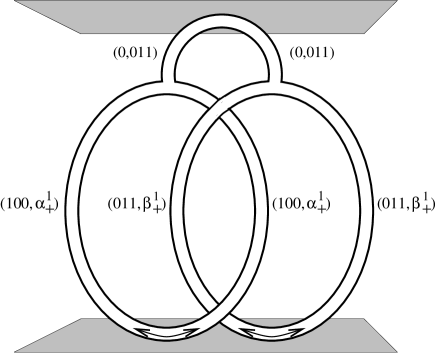
Figure 10: A dyon/anti-dyon pair $(100,\alpha^{1}_{+})$ and a dyon/anti-dyon pair $(011,\beta^{1}_{+})$ are created from the vacuum at a certain time slice. The ribbons represent the worldlines of the particles. After the dyon $(100,\alpha^{1}_{+})$ has encircled the flux $(011,\beta^{1}_{+})$, both particle/anti-particle pairs carry Cheshire charge $(0,011)$. These Cheshire charges become localized upon bringing the members of the pairs together again. Subsequently, the two charges $(0,011)$ annihilate each other.

From the fusion rules (8.42) and (8.43), respectively, we learn that a pair of dyons $(100,\alpha^{1}_{+})$ as well as a pair of dyons $(011,\beta^{1}_{+})$ can carry three different types of nontrivial Cheshire charge [9, 13, 15, 19, 62]. The nondiagonal form of the matrix (8.36) then implies that these two different pairs exchange Cheshire charge when a particle in one pair encircles a particle in the other pair. Consider, for instance, the process depicted in figure 10 in which a certain timeslice sees the creation of a $(100,\alpha^{1}_{+})$ dyon/anti-dyon pair and a $(011,\beta^{1}_{+})$ dyon/anti-dyon pair from the vacuum. Hence, both pairs carry a trivial Cheshire charge at this stage, i.e. both pairs are in the vacuum channel $(0)$ of their fusion rule. After the monodromy involving a dyon in the pair $(100,\alpha^{1}_{+})$ and a dyon in the pair $(011,\beta^{1}_{+})$, both pairs carry the nonlocalizable Cheshire charge $(0,011)$ which become localized charges upon fusing the members of the pairs. As follows from the rule (8.41), these localized charges annihilate each other when they are brought together. Hence, as it should, global ${\mbox{\bf Z}}_{2}\times{\mbox{\bf Z}}_{2}\times{\mbox{\bf Z}}_{2}$ charge is conserved in this process. All this becomes clear upon writing the process described above in terms of the associated internal quantumstates:

$$|0\rangle \longmapsto \frac{1}{2}\{|100,\left(\begin{array}[]{c}1\\ 0\end{array}\right)\rangle|100,\left(\begin{array}[]{c}1\\ 0\end{array}\right)\rangle\;+\;|100,\left(\begin{array}[]{c}0\\ 1\end{array}\right)\rangle|100,\left(\begin{array}[]{c}0\\ 1\end{array}\right)\rangle\}\otimes\qquad$$ (8.64)

$$\otimes\{|011,\left(\begin{array}[]{c}1\\ 0\end{array}\right)\rangle|011,\left(\begin{array}[]{c}0\\ 1\end{array}\right)\rangle\;+\;|011,\left(\begin{array}[]{c}0\\ 1\end{array}\right)\rangle|011,\left(\begin{array}[]{c}1\\ 0\end{array}\right)\rangle\}\qquad$$

$$\stackrel{{\scriptstyle{\mbox{\scriptsize\bf 1}}\otimes{\cal R}^{2}\otimes{\mbox{\scriptsize\bf 1}}}}{{\longmapsto}} \frac{1}{2}\{|100,\left(\begin{array}[]{c}1\\ 0\end{array}\right)\rangle|100,\left(\begin{array}[]{c}0\\ 1\end{array}\right)\rangle\;-\;|100,\left(\begin{array}[]{c}0\\ 1\end{array}\right)\rangle|100,\left(\begin{array}[]{c}1\\ 0\end{array}\right)\rangle\}\otimes\qquad$$

$$\otimes\{|011,\left(\begin{array}[]{c}0\\ 1\end{array}\right)\rangle|011,\left(\begin{array}[]{c}1\\ 0\end{array}\right)\rangle\;-\;|011,\left(\begin{array}[]{c}1\\ 0\end{array}\right)\rangle|011,\left(\begin{array}[]{c}0\\ 1\end{array}\right)\rangle\}\qquad$$

$$\longmapsto |0,011\rangle\otimes|0,011\rangle$$

$$\longmapsto |0\rangle\,.$$

The quasi-quantum double $D^{\omega_{\mbox{\tiny III}}}({\mbox{\bf Z}}_{2}\times{\mbox{\bf Z}}_{2}\times{\mbox{\bf Z}}_{2})$ acts on the two particle state (8.64) for the dyons $(100,\alpha^{1}_{+})$ through the comultiplication (5.4) with the 2-cocycle (8.2). From the action of the flux projection operators, we obtain that this state carries trivial total flux. Further, the global symmetry transformations, which act by means of the matrices (8.8), leave this two particle state invariant. So, this state indeed carries trivial total ${\mbox{\bf Z}}_{2}\times{\mbox{\bf Z}}_{2}\times{\mbox{\bf Z}}_{2}$ charge. In a similar fashion, we infer that the two particle state (8.64) for the dyons $(011,\beta^{1}_{+})$ corresponds to trivial total flux and charge. After the monodromy, which involves the matrix (8.36), both two particle states then carry the global charge $(0,011)$. Note that just as in the analogous process in the $\bar{D}_{2}$ theory discussed in [9] this exchange of Cheshire charge is accompanied by an exchange of quantum statistics. That is to say, the two particle states (8.64) and (8.64) are bosonic in accordance with the trivial spin (8.11) assigned to the dyons $(100,\alpha^{1}_{+})$ and $(011,\beta^{1}_{+})$ respectively. Both two particle states emerging after the monodromy, in turn, are fermionic.

As has been explained in section 5, the internal Hilbert space for a multi-particle system in an abelian discrete (CS) theory carries a representation of the direct product of the associated (quasi-) quantum double and some truncated braid group defined in appendix B. In the remainder of this subsection, I identify the truncated braid groups showing up in this particular type III ${\mbox{\bf Z}}_{2}\times{\mbox{\bf Z}}_{2}\times{\mbox{\bf Z}}_{2}$ CS theory and elaborate on the decomposition of the internal Hilbert space for some representative 3-particle systems into a direct some of irreducible subspaces under the action of the direct product of the quasi-quantum double $D^{\omega_{\mbox{\tiny III}}}({\mbox{\bf Z}}_{2}\times{\mbox{\bf Z}}_{2}\times{\mbox{\bf Z}}_{2})$ and the related truncated braid group. I start with the identical particle systems.

In fact, the only identical particle systems that obey nontrivial braid statistics in this model are those that consist either of the dyons $(111,\gamma_{+})$ or of the dyons $(111,\gamma_{-})$. It is easily verified that the braid operator (5.16) for these systems is of order $4$. Hence, the internal Hilbert space for a system containing $n$ of such identical dyons carries a representation of the truncated braid group $B(n,4)$ which is in general reducible, i.e. it decomposes into a direct sum of UIR’s. The one dimensional UIR’s that may occur in this decomposition then correspond to semion statistics, whereas the higher dimensional UIR’s correspond to nonabelian braid statistics. All other identical particle systems realize permutation statistics. That is, the associated truncated braid groups boil down to the permutation group. Specifically, the pure charges $(0,n^{(1)}n^{(2)}n^{(3)})$ are bosons, which is in accordance with the canonical spin statistics connection (5.37), since there is a trivial spin factor (8.11) assigned to these particles. Finally, the remaining dyons in general obey bose, fermi or parastatistics.

As an example of an identical particle system, I consider a system consisting of 3 dyons $(111,\gamma_{+})$. From the fusion rule (8.44) and the rules

$$(111,\gamma_{+})\times(0,011)\;=\;(111,\gamma_{+})\times(0,101)\;=\;(111,\gamma_{+})\times(0,101)\;=\;(111,\gamma_{-})\,,$$

one obtains that the associated 3-particle internal Hilbert space decomposes into the following irreducible pieces under the action of $D^{\omega_{\mbox{\tiny III}}}({\mbox{\bf Z}}_{2}\times{\mbox{\bf Z}}_{2}\times{\mbox{\bf Z}}_{2})$

$$(111,\gamma_{+})\times(111,\gamma_{+})\times(111,\gamma_{+}) = 4\;(111,\gamma_{-})\,.$$ (8.83)

According to the general discussion at the end of section 5.2, the occurrence of four isotypical fusion channels indicates that nonabelian braid statistics is conceivable for this identical particle system. Indeed, higher dimensional UIR’s of the related truncated braid group $B(3,4)$ appear. The 96 elements of $B(3,4)$ are divided into 16 conjugacy classes as displayed in relation (B.7) of appendix B. The matrices assigned to these elements in the representation of $B(3,4)$ realized by this distinguishable particle system follow from the relations (5.22), (3.8), (8.2) and (8.10). A lengthy but straightforward calculation of the trace of an arbitrary representative for each of the 16 conjugacy classes in (B.7) and a subsequent evaluation of the innerproduct of the resulting character vector with those for the UIR’s of $B(3,4)$ displayed in table 1 of appendix B then reveals that the $B(3,4)$ representation carried by the internal Hilbert space of this system breaks up into the following irreducible pieces

$$\Lambda_{B(3,4)} = 4\;\Lambda_{3}+2\;\Lambda_{5}\,.$$ (8.84)

Here, $\Lambda_{3}$ denotes the 1-dimensional UIR and $\Lambda_{5}$ the 2-dimensional UIR of $B(3,4)$ defined in character table 1. From (8.83) and (8.84), we now conclude that under the action of the direct product $D^{\omega_{\mbox{\tiny III}}}({\mbox{\bf Z}}_{2}\times{\mbox{\bf Z}}_{2}\times{\mbox{\bf Z}}_{2})\times B(3,4)$ the internal Hilbert space for a system of three dyons $(111,\gamma_{+})$ decomposes into the following irreducible pieces

$$2\;((111,\gamma_{-}),\Lambda_{3})\>+\>((111,\gamma_{-}),\Lambda_{5})\,,$$ (8.85)

where $((111,\gamma_{-}),\Lambda_{3})$ stands for a 2-dimensional representation and $((111,\gamma_{-}),\Lambda_{5})$ for a 4-dimensional representation. Further, from relation (B.7) and table 1 in appendix B, we learn that the generators $\tau_{1}$ and $\tau_{2}$ of $B(3,4)$ are represented by the scalar $-\imath$ in the representation $\Lambda_{3}$, which coincides with the spin factor (8.11) assigned to the dyon $(111,\gamma_{+})$. Thus the 3-particle states in the irreducible components $((111,\gamma_{-}),\Lambda_{3})$ in (8.85) satisfy the canonical spin-statistics connection (5.37). In passing, I just mention that an analogous calculation shows that the internal Hilbert space for a system of three dyons $(111,\gamma_{-})$ decomposes into the following irreducible subspaces under the action of $D^{\omega_{\mbox{\tiny III}}}({\mbox{\bf Z}}_{2}\times{\mbox{\bf Z}}_{2}\times{\mbox{\bf Z}}_{2})\times B(3,4)$

$$2\;((111,\gamma_{+}),\Lambda_{1})\>+\>((111,\gamma_{+}),\Lambda_{5})\,,$$ (8.86)

with $\Lambda_{1}$ the complex conjugate of the 1-dimensional UIR $\Lambda_{3}$ of $B(3,4)$ in (8.84).

Let me finally also briefly comment on the distinguishable particle systems in this theory. It is readily checked that the maximal order of the monodromy operator for distinguishable particles in this theory is 4. So, the distinguishable particles configurations in this theory realize representations of the truncated colored braid group $P(n,8)$ and its subgroups. The order of the two monodromy operators for a system consisting of the three dyons $(100,\alpha^{1}_{+})$, $(010,\alpha^{2}_{+})$ and $(001,\alpha^{3}_{+})$, for instance, is of order 2. Hence, the associated truncated colored braid group is $P(3,4)\subset P(3,8)$ discussed in appendix B. It consists of 16 elements organized into 10 conjugacy classes as displayed in relation (B.14). The matrices assigned to these elements in the representation of $P(3,4)$ realized by this 3-particle system now follow from the relations (B.8), (5.22), and (8.8). In a similar fashion as before, it is readily inferred that the $P(3,4)$ representation carried by the internal Hilbert space of this system breaks up into the following irreducible pieces

$$\Lambda_{P(3,4)} = 2\;\Omega_{8}+2\;\Omega_{9}\,,$$ (8.87)

with $\Omega_{8}$ and $\Omega_{9}$ the two dimensional UIR’s in the character table 2 of appendix B. To proceed, from the fusion rules (8.45) and (8.46), we learn that under the action of $D^{\omega_{\mbox{\tiny III}}}({\mbox{\bf Z}}_{2}\times{\mbox{\bf Z}}_{2}\times{\mbox{\bf Z}}_{2})$, the internal Hilbert space for this 3-particle system decomposes into the following direct sum of 4 irreducible representations

$$(100,\alpha^{1}_{+})\times(010,\alpha^{2}_{+})\times(001,\alpha^{3}_{+}) = 2\;(111,\gamma_{+})+2\;(111,\gamma_{-})\,.$$ (8.88)

To conclude, by constructing a basis adapted to the simultaneous decomposition of this 3-particle internal Hilbert space, it can be verified that the two UIR’s $\Omega_{8}$ of $P(3,4)$ in (8.87) combine with the two UIR’s $(111,\gamma_{+})$ of $D^{\omega_{\mbox{\tiny III}}}({\mbox{\bf Z}}_{2}\times{\mbox{\bf Z}}_{2}\times{\mbox{\bf Z}}_{2})$ in (8.88) and the two UIR’s $\Omega_{9}$ with the two UIR’s $(111,\gamma_{-})$. So, this internal Hilbert space system decomposes into the following irreducible subspaces

$$\left((111,\gamma_{+}),\Omega_{8}\right)\>+\>\left((111,\gamma_{-}),\Omega_{9}\right),$$ (8.89)

under the action of the direct product $D^{\omega_{\mbox{\tiny III}}}({\mbox{\bf Z}}_{2}\times{\mbox{\bf Z}}_{2}\times{\mbox{\bf Z}}_{2})\times P(3,4)$, where $\left((111,\gamma_{+}),\Omega_{8}\right)$ and $\left((111,\gamma_{-}),\Omega_{9}\right)$ both label a four dimensional representation.

8.3 Electric/magnetic duality

The analysis of the previous subsections revealed some striking similarities between the type III CS theory with gauge group ${\mbox{\bf Z}}_{2}\times{\mbox{\bf Z}}_{2}\times{\mbox{\bf Z}}_{2}$ and the ordinary discrete gauge theory with nonabelian finite gauge group the double dihedral group $\bar{D}_{2}$ discussed in full detail in [9, 35]. See also [15, 18, 19]. First of all, the orders of these gauge groups are the same: $|{\mbox{\bf Z}}_{2}\times{\mbox{\bf Z}}_{2}\times{\mbox{\bf Z}}_{2}|=|\bar{D}_{2}|=8$. Moreover, including the vacuum, the spectrum of both theories consists of $8$ singlet particles and $14$ doublet particles which adds up to a total number of 22 distinct particles. Also, the charge conjugation operation acts trivially on these spectra: ${\cal C}=S^{2}={\mbox{\bf 1}}$. That is, the particles in both theories are their own anti-particle. Finally, the truncated braid groups that govern the particle exchanges in these discrete gauge theories are similar. Hence, it seems that these theories are dual. As it stands, however, this is not the case. This becomes clear upon comparing the spins of the particles in the two different theories. The spin factors assigned to the particles in the $\bar{D}_{2}$ gauge theory can be found in Eq. (3.1.2) of reference [9]. In particular, there are three particles with spin factor $\imath$ and three particles with spin factor $-\imath$. As displayed in (8.11), the spectrum of the ${\mbox{\bf Z}}_{2}\times{\mbox{\bf Z}}_{2}\times{\mbox{\bf Z}}_{2}$ CS theory of type III, in contrast, contains just one particle with spin factor $\imath$ and one with $-\imath$. Hence, the modular $T$ matrices associated to these models differ. Moreover, it can be verified that the modular $S$ matrices classifying the monodromy properties of the particles in these theories are also distinct.

Let me now recall from (3.12) that the full set of CS actions for the gauge group ${\mbox{\bf Z}}_{2}\times{\mbox{\bf Z}}_{2}\times{\mbox{\bf Z}}_{2}$ consists of three nontrivial 3-cocycles (3.2) of type I, three 3-cocycles (3.2) of type II, one 3-cocycle (8.1) of type III and products thereof. It turns out that the ${\mbox{\bf Z}}_{2}\times{\mbox{\bf Z}}_{2}\times{\mbox{\bf Z}}_{2}$ CS theories corresponding to the product of the 3-cocycle of type III and either one of the three 3-cocycles of type I are, in fact, dual to a $\bar{D}_{2}$ gauge theory. Here, I just explicitly show this duality for the ${\mbox{\bf Z}}_{2}\times{\mbox{\bf Z}}_{2}\times{\mbox{\bf Z}}_{2}$ CS theory defined by

$$\omega_{\mbox{\scriptsize{I+III}}}(A,B,C) = \exp\left(\frac{\pi\imath}{2}a^{(1)}(b^{(1)}+c^{(1)}-[b^{(1)}+c^{(1)}])+\pi\imath\,a^{(1)}b^{(2)}c^{(3)}\right).\qquad$$ (8.90)

So the total CS action is the product of the 3-cocycle (8.1) of type III and the nontrivial 3-cocycle (3.2) of type I for the first ${\mbox{\bf Z}}_{2}$ gauge group in ${\mbox{\bf Z}}_{2}\times{\mbox{\bf Z}}_{2}\times{\mbox{\bf Z}}_{2}$. As indicated by (5.13), (5.9) and (3.21), adding this type I 3-cocycle to the $\{{\mbox{\bf Z}}_{2}\times{\mbox{\bf Z}}_{2}\times{\mbox{\bf Z}}_{2},\omega_{\mbox{\scriptsize{III}}}\}$ CS theory implies the assignment of an additional imaginary spin factor $\imath$ to those dyons in the spectrum (8.11) that carry nontrivial flux w.r.t.  the first ${\mbox{\bf Z}}_{2}$ gauge group of the product ${\mbox{\bf Z}}_{2}\times{\mbox{\bf Z}}_{2}\times{\mbox{\bf Z}}_{2}$. The spin factors of the other particles are unaffected. Thus the spin factors associated to the different particles in the $\{{\mbox{\bf Z}}_{2}\times{\mbox{\bf Z}}_{2}\times{\mbox{\bf Z}}_{2},\omega_{\mbox{\scriptsize{I+III}}}\}$ CS theory become

$$\begin{array}[]{cc}\mbox{particle}&\qquad\exp(2\pi\imath s)\\ (0,n^{(1)}n^{(2)}n^{(3)})&\qquad 1\\ (011,\beta^{1}_{\pm}),\,(010,\alpha^{2}_{\pm}),\,(001,\alpha^{3}_{\pm})&\qquad\pm 1\\ (100,\alpha^{1}_{\pm}),\,(101,\beta^{2}_{\pm}),\,(110,\beta^{3}_{\pm})&\qquad\pm\imath\\ (111,\gamma_{\pm})&\qquad\pm 1\,.\end{array}$$ (8.91)

Note that the spin structure of the spectrum of this theory indeed matches that of the $\bar{D}_{2}$ gauge theory exhibited in Eq. (3.1.2) of reference [9]. Moreover, it is readily checked that the modular $S$ matrix (5.27) for this ${\mbox{\bf Z}}_{2}\times{\mbox{\bf Z}}_{2}\times{\mbox{\bf Z}}_{2}$ CS theory is also equivalent to that for the $\bar{D}_{2}$ theory given in table 3.3 of reference [9]. To be explicit, the exchange

$$\bar{D}_{2} \longleftrightarrow \{{\mbox{\bf Z}}_{2}\times{\mbox{\bf Z}}_{2}\times{\mbox{\bf Z}}_{2},\omega_{\mbox{\scriptsize{I+III}}}\}\,,$$ (8.92)

which involves the following interchange of the particles in the $\bar{D}_{2}$ theory  with the particles (8.91) in the $\{{\mbox{\bf Z}}_{2}\times{\mbox{\bf Z}}_{2}\times{\mbox{\bf Z}}_{2},\omega_{\mbox{\scriptsize{I+III}}}\}$ CS theory

$$\begin{array}[]{rclrcl}1&\longleftrightarrow&(0)\,,&\qquad\bar{1}&\longleftrightarrow&(0,100)\\ J_{1}&\longleftrightarrow&(0,011)\,,&\qquad\bar{J}_{1}&\longleftrightarrow&(0,111)\\ J_{2}&\longleftrightarrow&(0,101)\,,&\qquad\bar{J}_{2}&\longleftrightarrow&(0,001)\\ J_{3}&\longleftrightarrow&(0,110)\,,&\qquad\bar{J}_{3}&\longleftrightarrow&(0,010)\\ \chi&\longleftrightarrow&(111,\gamma_{+})\,,&\qquad\bar{\chi}&\longleftrightarrow&(111,\gamma_{-})\\ \sigma^{\pm}_{1}&\longleftrightarrow&(011,\beta^{1}_{\pm})\,,&\qquad\tau^{\pm}_{1}&\longleftrightarrow&(100,\alpha^{1}_{\pm})\\ \sigma^{\pm}_{2}&\longleftrightarrow&(010,\alpha^{2}_{\pm})\,,&\qquad\tau^{\pm}_{2}&\longleftrightarrow&(101,\beta^{2}_{\pm})\\ \sigma^{\pm}_{3}&\longleftrightarrow&(001,\alpha^{3}_{\pm})\,,&\qquad\tau^{\pm}_{3}&\longleftrightarrow&(110,\beta^{3}_{\pm})\,,\end{array}$$ (8.101)

corresponds to an invariance of the modular matrices:

$$S_{\bar{D}_{2}}\;=\;S_{\{\mbox{\scriptsize\bf Z}_{2}\times\mbox{\scriptsize\bf Z}_{2}\times\mbox{\scriptsize\bf Z}_{2},\,\omega_{\mbox{\tiny{I+III}}}\}}\,,\qquad T_{\bar{D}_{2}}\;=\;T_{\{\mbox{\scriptsize\bf Z}_{2}\times\mbox{\scriptsize\bf Z}_{2}\times\mbox{\scriptsize\bf Z}_{2},\,\omega_{\mbox{\tiny{I+III}}}\}}\,.$$ (8.102)

Hence, these two theories are dual; they describe the same spectrum and the same topological interactions.

A couple of remarks concerning the foregoing duality are in order. To start with, the duality transformation (8.101) exchanges the nonabelian $\bar{D}_{2}$ magnetic flux doublets with the projective ${\mbox{\bf Z}}_{2}\times{\mbox{\bf Z}}_{2}\times{\mbox{\bf Z}}_{2}$ doublet dyon charges, while the ${\mbox{\bf Z}}_{4}$ singlet dyon charges associated to these $\bar{D}_{2}$ doublet fluxes are exchanged with the abelian ${\mbox{\bf Z}}_{2}\times{\mbox{\bf Z}}_{2}\times{\mbox{\bf Z}}_{2}$ magnetic fluxes. Also, the pure $\bar{D}_{2}$ singlet flux $\bar{1}$ is exchanged with the pure ${\mbox{\bf Z}}_{2}\times{\mbox{\bf Z}}_{2}\times{\mbox{\bf Z}}_{2}$ charge $(0,100)$. In short, we are dealing with some kind of nonabelian electric/magnetic duality. It should be stressed though that the interchange of electric and magnetic quantum numbers does not extend to the other particles. That is, the pure $\bar{D}_{2}$ singlet charges $J_{1}$, $J_{2}$ and $J_{3}$ and the singlet dyons $\bar{J}_{1}$, $\bar{J}_{2}$ and $\bar{J}_{3}$ are exchanged with pure ${\mbox{\bf Z}}_{2}\times{\mbox{\bf Z}}_{2}\times{\mbox{\bf Z}}_{2}$ singlet charges, the pure doublet charge $\chi$ with the doublet dyon $(111,\gamma_{+})$, while the singlet flux of the dyon $\bar{\chi}$ is exchanged with the singlet flux of the dyon $(111,\chi_{-})$ and the doublet dyon charge of $\bar{\chi}$ with the doublet dyon charge $\gamma_{-}$. As a next remark, the duality of the ${\mbox{\bf Z}}_{2}\times{\mbox{\bf Z}}_{2}\times{\mbox{\bf Z}}_{2}$ gauge theories with CS action the product of the 3-cocycle of type III and either one of the other two 3-cocycles (3.2) of type I with the $\bar{D}_{2}$ theory is inferred in a similar way. The duality transformation for these cases is given by a natural permutation of that in (8.101). Furthermore, it can be checked that duality with the $\bar{D}_{2}$ theory also emerges for the ${\mbox{\bf Z}}_{2}\times{\mbox{\bf Z}}_{2}\times{\mbox{\bf Z}}_{2}$ gauge theory featuring the CS action $\omega_{\mbox{\scriptsize I+I+I+III}}$, but is lost for the case $\omega_{\mbox{\scriptsize I+I+III}}$. Here, $\omega_{\mbox{\scriptsize I+I+I+III}}$ denotes the product of the three distinct 3-cocycles of type I and the 3-cocycle of type III, while $\omega_{\mbox{\scriptsize I+I+III}}$ stands for a product of two distinct 3-cocycles of type I and the 3-cocycle of type III. It is easily verified that the spin structure of the spectrum for the latter theory is not matching that of the $\bar{D}_{2}$ theory, since the spectrum for $\omega_{\mbox{\scriptsize I+I+III}}$ contains five dyons with spin factor $\imath$ and five dyons with spin factor $-\imath$. Finally, besides the double dihedral group $\bar{D}_{2}$ also the other nonabelian group of order 8 enters the scene, namely the dihedral group $D_{4}$. As we will argue next, the ${\mbox{\bf Z}}_{2}\times{\mbox{\bf Z}}_{2}\times{\mbox{\bf Z}}_{2}$ gauge theory with the type III CS action (8.1) itself, for instance, is dual to the ordinary 2+1 dimensional $D_{4}$ gauge theory discussed in appendix C. In fact, our earlier observation that the sets of matrices (8.8) and (8.9) associated to the dyon charges $\alpha^{i}_{\pm}$ and $\beta^{i}_{\pm}$, respectively, generate the two dimensional UIR of $D_{4}$ already formed circumstantial evidence supporting this result.

As displayed in relation (C.19) of appendix C, the $D_{4}$ theory features fourteen particles with trivial spin factor 1, six particles with spin factor $-1$, one with spin factor $\imath$ and one with $-\imath$. So, the spin structure (and thus the modular $T$ matrix) of the $D_{4}$ theory is the same as that given in relation (8.11) for the $\{{\mbox{\bf Z}}_{2}\times{\mbox{\bf Z}}_{2}\times{\mbox{\bf Z}}_{2},\omega_{\mbox{\scriptsize III}}\}$ CS theory. In addition, it can be verified that the modular $S$ matrix (5.27) for the $\{{\mbox{\bf Z}}_{2}\times{\mbox{\bf Z}}_{2}\times{\mbox{\bf Z}}_{2},\omega_{\mbox{\scriptsize III}}\}$ CS theory is equivalent to that for the $D_{4}$ theory exhibited in table 5 of appendix C. Specifically, the duality transformation $D_{4}\leftrightarrow\{{\mbox{\bf Z}}_{2}\times{\mbox{\bf Z}}_{2}\times{\mbox{\bf Z}}_{2},\omega_{\mbox{\scriptsize III}}\}$ for this case involves the following exchange of the particles in the spectrum (C.10) of the $D_{4}$ theory with the particles (8.11) featuring in the $\{{\mbox{\bf Z}}_{2}\times{\mbox{\bf Z}}_{2}\times{\mbox{\bf Z}}_{2},\omega_{\mbox{\scriptsize III}}\}$ CS theory

$$\begin{array}[]{rclrcl}(0,++)&\longleftrightarrow&(0)\,,&\qquad(2,++)&\longleftrightarrow&(0,111)\\ (0,+-)&\longleftrightarrow&(0,011)\,,&\qquad(2,+-)&\longleftrightarrow&(0,100)\\ (0,-+)&\longleftrightarrow&(0,010)\,,&\qquad(2,-+)&\longleftrightarrow&(0,101)\\ (0,--)&\longleftrightarrow&(0,001)\,,&\qquad(2,--)&\longleftrightarrow&(0,110)\\ (0,1)&\longleftrightarrow&(100,\alpha^{1}_{+})\,,&\qquad(2,1)&\longleftrightarrow&(100,\alpha^{1}_{-})\\ (1,0)&\longleftrightarrow&(011,\beta^{1}_{+})\,,&(X,\pm+)&\longleftrightarrow&(101,\beta^{2}_{\pm})\\ (1,1)&\longleftrightarrow&(111,\gamma_{-})\,,&(X,\pm-)&\longleftrightarrow&(001,\alpha^{3}_{\pm})\\ (1,2)&\longleftrightarrow&(011,\beta^{1}_{-})\,,&(\bar{X},\pm+)&\longleftrightarrow&(110,\beta^{3}_{\pm})\\ (1,3)&\longleftrightarrow&(111,\gamma_{+})\,,&(\bar{X},\pm-)&\longleftrightarrow&(010,\alpha^{2}_{\pm})\,.\end{array}$$ (8.112)

To proceed, a straightforward calculation shows that adding either one of the three 3-cocycles (3.2) of type II to the $\{{\mbox{\bf Z}}_{2}\times{\mbox{\bf Z}}_{2}\times{\mbox{\bf Z}}_{2},\omega_{\mbox{\scriptsize III}}\}$ CS theory does not destruct the duality with the $D_{4}$ theory. That is, we also have the duality $D_{4}\leftrightarrow\{{\mbox{\bf Z}}_{2}\times{\mbox{\bf Z}}_{2}\times{\mbox{\bf Z}}_{2},\omega_{\mbox{\scriptsize II+III}}\},$ where the associated duality transformation between the two spectra again corresponds to a permutation of the one in (8.112).

To conclude, a complete discussion, which is beyond the scope of this paper, also involves the finite set of CS actions for the two nonabelian gauge groups $D_{4}$ and $\bar{D}_{2}$. This and the generalization of the foregoing nonabelian dualities to higher order finite abelian gauge groups allowing for CS actions of type III is left for future work. An interesting question concerning the latter generalization is whether the nonabelian dual gauge groups are restricted to the dihedral and double dihedral series or also involve other nonabelian finite groups.

9 Dijkgraaf-Witten invariants

In reference [29], Dijkgraaf and Witten defined a topological invariant for a compact, closed oriented three manifold ${\cal M}$ in terms of a 3-cocycle $\omega\in H^{3}({H},U(1))$ for a finite group $H$. They represented this invariant as the partition function $Z({\cal M})$ of a lattice gauge theory with gauge group $H$ and CS action $\omega$. It was shown explicitly that $Z(M)$ is indeed a combinatorial invariant of the manifold ${\cal M}$. In this section, I present some results on the Dijkgraaf-Witten inavariant for lens spaces using the 3-cocycles of type II and of type III for a finite abelian group $H$, which to my knowledge have not appeared in the literature before. In addition, the value of the Dijkgraaf-Witten invariant for the 3-torus ${\cal M}=S^{1}\times S^{1}\times S^{1}$ associated with the three types of 3-cocycles for ${H}\simeq{\mbox{\bf Z}}_{2}\times{\mbox{\bf Z}}_{2}\times{\mbox{\bf Z}}_{2}$ is derived.

The Dijkgraaf-Witten invariant for the lens space $L(p,q)$ associated with an abelian finite group $H$ and 3-cocycle $\omega$ takes the following form [29, 38]

$$Z(L(p,q)) = \frac{1}{|{H}|}\sum_{\{A\in{H}|[A^{p}]=0\}}\;\;\prod_{j=1}^{p-1}\omega(A,A^{j},A^{n})\,,$$ (9.1)

with $|H|$ the order of $H$ and $n$ the inverse of $q$ mod $p$. It is known [38, 63] that the Dijkgraaf-Witten invariant for the 3-cocycles (3.2) of type I for ${H}\simeq{\mbox{\bf Z}}_{5}$ can distinguish the lens spaces $L(5,1)$ and $L(5,2)$, which are homeomorphic but of different homotopy type:

$$Z(L(5,1)) = \left\{\begin{array}[]{ll}1&\mbox{for $p_{\mbox{\scriptsize I}}=0$}\\ \frac{1}{\sqrt{5}}&\mbox{for $p_{\mbox{\scriptsize I}}=1,4$}\\ -\frac{1}{\sqrt{5}}&\mbox{for $p_{\mbox{\scriptsize I}}=2,3$}\end{array}\right.$$ (9.5)

$$Z(L(5,2)) = \left\{\begin{array}[]{cl}1&\mbox{for $p_{\mbox{\scriptsize I}}=0$}\\ -\frac{1}{\sqrt{5}}&\mbox{for $p_{\mbox{\scriptsize I}}=1,4$}\\ \frac{1}{\sqrt{5}}&\mbox{for $p_{\mbox{\scriptsize I}}=2,3$}\,.\end{array}\right.$$ (9.9)

A simple numerical evaluation using for example Mathematica shows that this nice property of the Dijkgraaf-Witten invariant (9.1) is lost for 3-cocycles of type II and III. Specifically, for ${H}\simeq{\mbox{\bf Z}}_{5}\times{\mbox{\bf Z}}_{5}$ and a 3-cocycle (3.2) of type II, one arrives at

$$Z(L(5,1))\;=\;Z(L(5,2))\;=\;\left\{\begin{array}[]{ll}1&\mbox{for $p_{\mbox{\scriptsize II}}=0$}\\ \frac{1}{5}&\mbox{for $p_{\mbox{\scriptsize II}}=1,\dots,4$}\,,\end{array}\right.$$ (9.12)

while for ${H}\simeq{\mbox{\bf Z}}_{5}\times{\mbox{\bf Z}}_{5}\times{\mbox{\bf Z}}_{5}$ and a 3-cocycle (3.2) of type III the situation becomes completely trivial

$$Z(L(5,1))\;=\;Z(L(5,2))\;=\;1\qquad\mbox{for $p_{\mbox{\scriptsize III}}=0,1,\ldots,4$}\,.$$ (9.13)

In fact, it turns out that in general the invariant (9.1) based on the 3-cocycles of type II and III have less distinctive power then the one based on 3-cocycles of type I. Further, the result for the nontrivial 3-cocycle of type I for ${H}\simeq{\mbox{\bf Z}}_{2}$

$$Z(L(p,1)) = \left\{\begin{array}[]{ll}\frac{1}{2}&\mbox{for odd $p$}\\ \frac{1}{2}(1+(-1)^{p/2})&\mbox{for even $p$}\,,\end{array}\right.$$ (9.16)

established in [29], generalizes in the following manner to the nontrivial 3-cocycle (3.2) of type II for ${H}\simeq{\mbox{\bf Z}}_{2}\times{\mbox{\bf Z}}_{2}$

$$Z(L(p,1)) = \left\{\begin{array}[]{ll}\frac{1}{4}&\mbox{for odd $p$}\\ \frac{1}{4}(3+(-1)^{p/2})&\mbox{for even $p$}\,,\end{array}\right.$$ (9.19)

and to

$$Z(L(p,1)) = \left\{\begin{array}[]{ll}\frac{1}{8}&\mbox{for odd $p$}\\ \frac{1}{8}(7+(-1)^{p/2})&\mbox{for even $p$}\,,\end{array}\right.$$ (9.22)

for the nontrivial 3-cocycle (3.2) of type III for ${H}\simeq{\mbox{\bf Z}}_{2}\times{\mbox{\bf Z}}_{2}\times{\mbox{\bf Z}}_{2}$.

The Dijkgraaf-Witten invariant for the 3-torus $S^{1}\times S^{1}\times S^{1}$ is of particular interest, since it counts the number of particles in the spectrum of a discrete ${H}$ CS gauge theory [29]. For abelian groups ${H}$ it takes the form

$$Z(S^{1}\times S^{1}\times S^{1}) = \frac{1}{|{H}|}\sum_{A,B,C\in{H}}W(A,B,C)\,,$$ (9.23)

with

$$W(A,B,C) = \frac{\omega(A,B,C)\;\omega(B,C,A)\;\omega(C,A,B)}{\omega(A,C,B)\;\omega(B,A,C)\;\omega(C,B,A)}\,.$$ (9.24)

It is not difficult to check that for the three different types of 3-cocycles for the direct product group ${H}\simeq{\mbox{\bf Z}}_{2}\times{\mbox{\bf Z}}_{2}\times{\mbox{\bf Z}}_{2}$, the invariant takes the values

$$Z(S^{1}\times S^{1}\times S^{1}) = \left\{\begin{array}[]{cl}64&\mbox{for type~{}I and~{}II}\\ 22&\mbox{for type~{}III}\,,\end{array}\right.$$ (9.27)

expressing the collapse of the spectrum we found for 3-cocycles of type III in section 8.

As an aside, with the same data entering the Dijkgraaf-Witten invariant, namely a finite group ${H}$ and a 3-cocycle $\omega$, Altschuler and Coste [38, 63] constructed a surgery invariant ${\cal F}({\cal M})$ from a surgery presentation of the manifold ${\cal M}$. They conjectured that up to normalization these two invariants are the same. That is, ${\cal F}({\cal M)}=Z({\cal M})/Z(S^{3})$ with $Z(S^{3})=1/|{H}|$. Altschuler and Coste verified their conjecture for lens spaces using the 3-cocycles of type I for cyclic groups ${H}\simeq{\mbox{\bf Z}}_{N}$. In [35], I subsequently reported that extending this analysis to the 3-cocycles of type II and of type III, which were not treated in [38, 63], did not lead to any counter–examples. In the meanwhile, I have become aware of reference [64] which contains the proof of the conjecture of Altschuler and Coste.

10 Concluding remarks and outlook

Some time ago Dijkgraaf and Witten [29] pointed out that the Chern-Simons (CS) actions for a compact gauge group $G$ are in one to one correspondence with the different elements of the cohomology group $H^{4}(BG,{\mbox{\bf Z}})$ with $BG$ the classifying space for $G$. They also noted that this classification includes the case of finite gauge groups $H$. The isomorphism $H^{4}(BH,{\mbox{\bf Z}})\simeq H^{3}(H,U(1))$, which only holds for finite $H$, then indicates that the different CS actions for a finite gauge group $H$ correspond to the inequivalent 3-cocycles $\omega\in H^{3}(H,U(1))$. One of the key results of the present paper has been that effective the long distance physics of a CS theory in which the gauge group $G$ is broken down to a subgroup $K$ via the Higgs mechanism is described by a CS theory with residual gauge group $K$ and CS action $S_{\mbox{\scriptsize CS}}^{\prime}\in H^{4}(BK,{\mbox{\bf Z}})$ determined by the original CS action $S_{\mbox{\scriptsize CS}}\in H^{4}(BG,{\mbox{\bf Z}})$ for the broken gauge group $G$ through the natural homomorphism $H^{4}(BG,{\mbox{\bf Z}})\rightarrow H^{4}(BK,{\mbox{\bf Z}})$ induced by the inclusion $K\subset G$. In case $G$ is broken down to a finite residual gauge group $H$, the foregoing homomorphism, also known as the restriction, and the aforementioned isomorphism $H^{4}(BH,{\mbox{\bf Z}})\simeq H^{3}(H,U(1))$ then combines into a natural homomorphism $H^{4}(BG,{\mbox{\bf Z}})\rightarrow H^{3}(H,U(1))$. The 3-cocycle $\omega\in H^{3}(H,U(1))$ being the image of some $S_{\mbox{\scriptsize CS}}\in H^{4}(BG,{\mbox{\bf Z}})$ under the latter mapping simply summarizes the additional Aharonov-Bohm (AB) interactions cast upon the magnetic vortices featuring in this model by the original CS action $S_{\mbox{\scriptsize CS}}$ for the broken gauge group $G$. This general scheme was illustrated with CS theories in which some continuous compact abelian gauge group, typically a direct product $G\simeq U(1)^{k}$ of $k$ compact $U(1)$ gauge groups, is spontaneously broken down to a finite subgroup being a direct product $H\simeq{\mbox{\bf Z}}_{N^{(1)}}\times{\mbox{\bf Z}}_{N^{(2)}}\times\cdots\times{\mbox{\bf Z}}_{N^{(k)}}$ with ${\mbox{\bf Z}}_{N^{(i)}}$ the cyclic group of order ${N^{(i)}}$. Among other things, it has been argued that the restriction $H^{4}(B(U(1)^{k}),{\mbox{\bf Z}})\rightarrow H^{3}({\mbox{\bf Z}}_{N^{(1)}}\times\cdots\times{\mbox{\bf Z}}_{N^{(k)}},U(1))$ accompanying this case is not onto. Specifically, there are two types of CS terms for $U(1)^{k}$. One type describes self couplings of the distinct $U(1)$ gauge fields, whereas the other type establishes pairwise couplings between the different $U(1)$ gauge fields. Further, in the presence of Dirac monopoles the topological masses characterizing these CS terms are necessarily quantized which is in agreement with the fact that the different CS actions for a compact gauge group $U(1)^{k}$ are labeled by the integers: $H^{4}(B(U(1)^{k}),{\mbox{\bf Z}})\simeq{\mbox{\bf Z}}^{k+\frac{1}{2}k(k-1)}$. The 3-cocycles for the direct product group ${\mbox{\bf Z}}_{N^{(1)}}\times\cdots\times{\mbox{\bf Z}}_{N^{(k)}}$, on the other hand, were shown to split up into three different types. The first type describes additional AB interactions between vortices carrying flux w.r.t. the same cyclic gauge group in the direct product, the second type between vortices belonging to two different cyclic gauge group in the direct product, and the third type realizes couplings between fluxes associated with three distinct cyclic gauge groups. It has been demonstrated that only the first two types of 3-cocycles can be obtained from a spontaneously broken $U(1)^{k}$ CS theory.

In fact, the 3-cocycles of the third type that can not be reached from the spontaneous breakdown of a $U(1)^{k}$ CS theory turned out to be the most interesting. Adding such a 3-cocycle or CS action to an abelian discrete $H$ gauge theory renders the theory nonabelian. Moreover, the ${\mbox{\bf Z}}_{2}\times{\mbox{\bf Z}}_{2}\times{\mbox{\bf Z}}_{2}$ CS theory defined by such a 3-cocycle, for instance, was shown to be dual to an ordinary $D_{4}$ gauge theory with $D_{4}$ the dihedral group of order 8, while the ${\mbox{\bf Z}}_{2}\times{\mbox{\bf Z}}_{2}\times{\mbox{\bf Z}}_{2}$ CS theory given by the product of a 3-cocycle of the first and third type was demonstrated to be dual to an ordinary $\bar{D}_{2}$ gauge theory with $\bar{D}_{2}$ the double dihedral group of order 8. The corresponding duality transformations involve the exchange of electric and magnetic quantum numbers. Future research should point out how these nonabelian electric/magnetic dualities generalize to higher order abelian finite gauge groups $H$. Another question that deserves further scrutiny is whether abelian discrete $H$ theories with a 3-cocycle of the third type can be embedded in CS theories with a nonabelian broken continuous gauge group.

The focus of the discussion of the type II $U(1)\times U(1)$ CS theory in section 7 was on the case in which both $U(1)$ gauge groups are simultaneously broken down to a cyclic group. Of course , it is also conceivable that just one $U(1)$ gauge group is broken to a cyclic group. A group cohomogical derivation for the latter case analogous to those in appendix A yields $H^{4}(B(U(1)\times{\mbox{\bf Z}}_{N}),{\mbox{\bf Z}})\simeq{\mbox{\bf Z}}\oplus{\mbox{\bf Z}}_{N}\oplus{\mbox{\bf Z}}_{N}$. Here, Z naturally labels the different type I CS actions for the compact $U(1)$ gauge group, one of the ${\mbox{\bf Z}}_{N}$ terms the 3-cocycles of type I for the finite cyclic gauge group ${\mbox{\bf Z}}_{N}$ and the other ${\mbox{\bf Z}}_{N}$ term the type II CS action for $U(1)\times{\mbox{\bf Z}}_{N}$. This results indicates that if one of the $U(1)$ groups of a type II $U(1)\times U(1)$ CS theory is spontaneously broken down to ${\mbox{\bf Z}}_{N}$ the integral type II CS parameter becomes periodic with period $N$. The characteristics of this model are currently under investigation.

Also, the vortices, pure charges and dyons in these spontaneously broken models have been treated as point particles in the first quantized description in this paper. Rerunning the discussion in the framework of canonical quantization involves the construction of magnetic vortex creation operators and charge creation operators and an analysis of their nontrivial commutation relations [65].

Another obvious next step is to consider CS theories in which some continuous nonabelian gauge group is spontaneously broken down to a finite nonabelian gauge group. For a concise discussion of these models, the reader is referred to [35] and references therein. A more detailed study will be presented elsewhere.

Finally, it has recently been suggested [20, 21] that $U(1)^{k}$ CS theories may play a role in multi-layered fractional quantum Hall systems. At present, it is not clear to me whether the broken version of these models considered in this paper are also relevant in this setting.

A Cohomological derivations

This appendix contains the derivation of some of the group cohomological results used in this paper. In passing, I stress that in contrast with the main text the cohomology and abelian groups will be presented in the additive rather than multiplicative form. In the additive presentation, a direct product of $k$ cyclic factors ${\mbox{\bf Z}}_{N}$, for example, becomes the direct sum denoted by ${\mbox{\bf Z}}_{N}^{k}:=\oplus_{i=1}^{k}{\mbox{\bf Z}}_{N}$.

My first objective is to prove the isomorphism (2.2). This will be done using the universal coefficients theorem (e.g. [67])

$$H^{n}(X,{\mbox{\bf B}}) \simeq H^{n}(X,{\mbox{\bf Z}})\otimes{\mbox{\bf B}}\oplus\mbox{Tor}(H^{n+1}(X,{\mbox{\bf Z}}),{\mbox{\bf B}})\,,$$ (A.1)

relating the cohomology of some topological space $X$ with coefficients in some abelian group B and the cohomology of $X$ with integer coefficients Z. Here, $\otimes$ stands for the symmetric tensor product and $\mbox{Tor}(\,.\,\,,\,.\,)$ for the torsion product. The symmetric tensor product ${\mbox{\bf A}}\otimes{\mbox{\bf B}}$ (over Z) for abelian groups A and B is the abelian group of all ordered pairs $a\otimes b$ ($a\in{\mbox{\bf A}}$ and $b\in{\mbox{\bf B}}$) with relations [67]

$$(a+a^{\prime})\otimes b = a\otimes b+a^{\prime}\otimes b,\qquad a\otimes(b+b^{\prime})\;=\;a\otimes b+a\otimes b^{\prime}$$

$$m(a\otimes b) = ma\otimes b\;=\;a\otimes mb\qquad\forall\,m\in{\mbox{\bf Z}}\,.$$

It is not difficult to check that these relations imply the following identifications

$${\mbox{\bf Z}}_{N}\otimes{\mbox{\bf Z}}_{M} \simeq {\mbox{\bf Z}}_{{\gcd}(N,M)}$$ (A.2)

$${\mbox{\bf Z}}_{N}\otimes{\mbox{\bf Z}} \simeq {\mbox{\bf Z}}_{N}$$ (A.3)

$${\mbox{\bf Z}}_{N}\otimes U(1) \simeq 0$$ (A.4)

$${\mbox{\bf Z}}\otimes U(1) \simeq U(1)$$ (A.5)

$${\mbox{\bf Z}}\otimes{\mbox{\bf Z}} \simeq {\mbox{\bf Z}}\,,$$ (A.6)

with ${\gcd}(N,M)$ the greatest common divisor of $N$ and $M$. Finally, the symmetric tensor product $\otimes$ is obviously distributive

$$(\oplus_{i}{\mbox{\bf A}}_{i})\otimes{\mbox{\bf B}} \simeq \oplus_{i}({\mbox{\bf A}}_{i}\otimes{\mbox{\bf B}})\,.$$ (A.7)

The definition of the torsion product $\mbox{Tor}(\,.\,\,,\,.\,)$ can be found in any textbook on algebraic topology. For our purposes, the following properties suffice [67]. Let A and B again be abelian groups, then

$$\mbox{Tor}({\mbox{\bf A}},{\mbox{\bf B}}) \simeq \mbox{Tor}({\mbox{\bf B}},{\mbox{\bf A}})$$

$$\mbox{Tor}({\mbox{\bf Z}}_{N},{\mbox{\bf B}}) \simeq {\mbox{\bf B}}[N]\;\simeq\;\{b\in{\,\mbox{\bf B}}\,|\,Nb=0\,\}\,,$$

so in particular

$$\mbox{Tor}({\mbox{\bf Z}}_{N},{\mbox{\bf Z}}_{M}) \simeq {\mbox{\bf Z}}_{{\gcd}(N,M)}$$ (A.8)

$$\mbox{Tor}({\mbox{\bf Z}}_{N},U(1)) \simeq {\mbox{\bf Z}}_{N}$$ (A.9)

$$\mbox{Tor}({\mbox{\bf A}},{\mbox{\bf Z}}) \simeq 0\qquad\qquad\forall{\mbox{\bf A}}\,.$$ (A.10)

The last identity follows from the fact that the group of integers Z is torsion free, i.e. it does not contain elements of finite order. Just as the symmetric tensor product, the torsion product is distributive

$$\mbox{Tor}(\oplus_{i}{\mbox{\bf A}}_{i},{\mbox{\bf B}}) \simeq \oplus_{i}\mbox{Tor}({\mbox{\bf A}}_{i},{\mbox{\bf B}})\,.$$ (A.11)

The proof of the isomorphism (2.2) now goes as follows. First we note that for finite groups ${H}$ all cohomology in fixed degree $n>0$ is finite. With this knowledge, the universal coefficients theorem (A.1) directly gives the desired result

$$H^{n}({H},U(1)) \simeq H^{n}({H},{\mbox{\bf Z}})\otimes U(1)\oplus\mbox{Tor}(H^{n+1}({H},{\mbox{\bf Z}}),U(1))$$ (A.12)

$$\simeq H^{n+1}({H},{\mbox{\bf Z}})\qquad\mbox{for $n>0$}\,.$$

In the last step, we used the distributive property of the tensor product (A.7) and the torsion product (A.11) together with the identities (A.4) and (A.9).

We turn to the derivation of the identities (3.10)–(3.12). Our starting point will be the standard result (e.g. [33])

$$H^{n}({\mbox{\bf Z}}_{N},{\mbox{\bf Z}}) \simeq \left\{\begin{array}[]{ll}{\mbox{\bf Z}}_{N}&\mbox{if $n$ is even}\\ 0&\mbox{if $n$ is odd}\\ {\mbox{\bf Z}}&\mbox{if $n=0\,,$}\end{array}\right.$$ (A.16)

which together with (A.12) implies that the identities in (3.10)–(3.12) are valid for $k=1$. The extension to $k>1$ involves the so-called Künneth formula (e.g. [67])

$$H^{n}(X\times Y,{\mbox{\bf Z}})\;\simeq\sum_{i+j=n}H^{i}(X,{\mbox{\bf Z}})\otimes H^{j}(Y,{\mbox{\bf Z}})\oplus\!\!\!\sum_{p+q=n+1}\!\!\!\mbox{Tor}(H^{p}(X,{\mbox{\bf Z}}),H^{q}(Y,{\mbox{\bf Z}}))\,,\;\;$$ (A.17)

which states that the cohomology of a direct product space is completely determined in terms of the cohomology of its factors. With the ingredients (A.16) and (A.17), the identities (3.10)–(3.12) can then be proven by induction. To lighten the notation a bit, we will omit explicit mention of the coefficients of the cohomology groups if the integers Z are meant. So, $H^{n}({\mbox{\bf Z}}_{N}^{k}):=H^{n}({\mbox{\bf Z}}_{N}^{k},{\mbox{\bf Z}})$. Let us start with the trivial cohomology group $H^{0}({\mbox{\bf Z}}_{N}^{k})$. Upon using the Künneth formula (A.17), the property (A.10) of the torsion product and the result (A.16), we easily infer

$$H^{0}({\mbox{\bf Z}}_{N}^{k})\;\simeq\;H^{0}({\mbox{\bf Z}}_{N}^{k-1})\otimes H^{0}({\mbox{\bf Z}}_{N}^{k})\;\simeq\;H^{0}({\mbox{\bf Z}}_{N}^{k-1})\otimes{\mbox{\bf Z}}\;\simeq\;{\mbox{\bf Z}}\,,$$ (A.18)

where the last isomorphism follows by induction. To be explicit, as indicated by (A.16) this isomorphism obviously holds for $k=1$. If we subsequently assume that this isomorphism is valid for some fixed $k$, we obtain with (A.6) that it also holds for $k+1$. To proceed, in a similar fashion, we arrive at

$$H^{1}({\mbox{\bf Z}}_{N}^{k})\;\simeq\;H^{1}({\mbox{\bf Z}}_{N}^{k-1})\otimes H^{0}({\mbox{\bf Z}}_{N})\;\simeq\;H^{1}({\mbox{\bf Z}}_{N}^{k-1})\;\simeq\;0\,.$$ (A.19)

These results enter the following derivation starting from the Künneth formula (A.17)

$$H^{2}({\mbox{\bf Z}}_{N}^{k}) \simeq H^{0}({\mbox{\bf Z}}_{N}^{k-1})\otimes H^{2}({\mbox{\bf Z}}_{N})\oplus H^{2}({\mbox{\bf Z}}_{N}^{k-1})\otimes H^{0}({\mbox{\bf Z}}_{N})$$

$$\simeq {\mbox{\bf Z}}_{N}\oplus H^{2}({\mbox{\bf Z}}_{N}^{k-1})\;\simeq\;{\mbox{\bf Z}}_{N}^{k}\,.$$

Here, we used the distributive property (A.7) of the tensor product and again induction to establish the last isomorphism. We continue with

$$H^{3}({\mbox{\bf Z}}_{N}^{k}) \simeq H^{3}({\mbox{\bf Z}}_{N}^{k-1})\otimes H^{0}({\mbox{\bf Z}}_{N})\oplus\mbox{Tor}(H^{2}({\mbox{\bf Z}}_{N}^{k-1}),H^{2}({\mbox{\bf Z}}_{N}))$$

$$\simeq H^{3}({\mbox{\bf Z}}_{N}^{k-1})\oplus{\mbox{\bf Z}}_{N}^{k-1}\;\simeq\;{\mbox{\bf Z}}_{N}^{\frac{1}{2}k(k-1)}\,.$$

Finally, using the previous results and induction, we obtain

$$H^{4}({\mbox{\bf Z}}_{N}^{k}) \simeq H^{0}({\mbox{\bf Z}}_{N}^{k-1})\otimes H^{4}({\mbox{\bf Z}}_{N})\oplus H^{2}({\mbox{\bf Z}}_{N}^{k-1})\otimes H^{2}({\mbox{\bf Z}}_{N})\oplus$$

$$H^{4}({\mbox{\bf Z}}_{N}^{k-1})\otimes H^{0}({\mbox{\bf Z}}_{N})\oplus\mbox{Tor}(H^{3}({\mbox{\bf Z}}_{N}^{k-1}),H^{2}({\mbox{\bf Z}}_{N}))$$

$$\simeq H^{4}({\mbox{\bf Z}}_{N})\oplus H^{2}({\mbox{\bf Z}}_{N}^{k-1})\oplus H^{4}({\mbox{\bf Z}}_{N}^{k-1})\oplus\mbox{Tor}(H^{3}({\mbox{\bf Z}}_{N}^{k-1}),H^{2}({\mbox{\bf Z}}_{N}))$$

$$\simeq {\mbox{\bf Z}}_{N}\oplus{\mbox{\bf Z}}_{N}^{k-1}\oplus H^{4}({\mbox{\bf Z}}_{N}^{k-1})\oplus{\mbox{\bf Z}}_{N}^{\frac{1}{2}(k-1)(k-2)}$$

$$\simeq {\mbox{\bf Z}}_{N}^{k+\frac{1}{2}(k-1)(k-2)}\oplus H^{4}({\mbox{\bf Z}}_{N}^{k-1})$$

$$\simeq {\mbox{\bf Z}}_{N}^{k+\frac{1}{2}k(k-1)+\frac{1}{3!}k(k-1)(k-2)}\,.$$

To conclude, the results (A), (A) and (A) together with (A.12) lead to the identities (3.10), (3.11) and (3.12) respectively.

The foregoing derivation also gives a nice insight into the structure of the terms building up the cohomology group $H^{4}({\mbox{\bf Z}}_{N}^{k})\simeq H^{3}({\mbox{\bf Z}}_{N}^{k},U(1))$. We can, in fact, distinguish three types of terms that contribute here. By induction, we find that there are $k$ terms of the form $H^{4}({\mbox{\bf Z}}_{N})$. These are the terms that label the 3-cocycles (3.2) of type I. By a similar argument, we infer that there are $\frac{1}{2}k(k-1)$ terms of the form $H^{2}({\mbox{\bf Z}}_{N}^{k-1})$. These terms label the type II 3-cocycles (3.2). Finally, the $\frac{1}{3!}k(k-1)(k-2)$ terms we are left with are entirely due to torsion products and label the 3-cocycles (3.2) of type III.

The generalization of the above results to abelian groups ${H}$ being direct products of cyclic groups possibly of different order is straightforward. The picture that the 3-cocycles divide into three different types remains unaltered. If the direct product ${H}$ consists of $k$ cyclic factors, then there are again $k$ different 3-cocycles of type I, $\frac{1}{2}k(k-1)$ different 3-cocycles of type II and $\frac{1}{3!}k(k-1)(k-2)$ different 3-cocycles of type III. The only distinction is that through (A.2) and (A.8) the greatest common divisors of the orders of the different cyclic factors constituting the direct product group $H$ enter the scene for 3-cocycles of type II and III. This is best illustrated by considering the direct product group $H\simeq{\mbox{\bf Z}}_{N}\times{\mbox{\bf Z}}_{M}\times{\mbox{\bf Z}}_{K}$ being the simplest example where all three types of 3-cocycles appear. The derivation (A.18)–(A) for this case leads to the following content of the relevant cohomology groups

$$\left\{\begin{array}[]{lcl}H^{1}({\mbox{\bf Z}}_{N}\times{\mbox{\bf Z}}_{M}\times{\mbox{\bf Z}}_{K},U(1))&\simeq&{\mbox{\bf Z}}_{N}\oplus{\mbox{\bf Z}}_{M}\oplus{\mbox{\bf Z}}_{K}\\ H^{2}({\mbox{\bf Z}}_{N}\times{\mbox{\bf Z}}_{M}\times{\mbox{\bf Z}}_{K},U(1))&\simeq&{\mbox{\bf Z}}_{{\gcd}(N,M)}\oplus{\mbox{\bf Z}}_{{\gcd}(N,K)}\oplus{\mbox{\bf Z}}_{{\gcd}(M,K)}\\ H^{3}({\mbox{\bf Z}}_{N}\times{\mbox{\bf Z}}_{M}\times{\mbox{\bf Z}}_{K},U(1))&\simeq&{\mbox{\bf Z}}_{N}\oplus{\mbox{\bf Z}}_{M}\oplus{\mbox{\bf Z}}_{K}\oplus\\ &&{\mbox{\bf Z}}_{{\gcd}(N,M)}\oplus{\mbox{\bf Z}}_{{\gcd}(N,K)}\oplus{\mbox{\bf Z}}_{{\gcd}(M,K)}\oplus\\ &&{\mbox{\bf Z}}_{{\gcd}(N,M,K)}\,.\end{array}\right.$$ (A.28)

The 3-cocycles of type I labeled by the terms ${\mbox{\bf Z}}_{N}$, ${\mbox{\bf Z}}_{M}$ and ${\mbox{\bf Z}}_{K}$ are of the form (3.16), whereas the explicit the 3-cocycles of type II labeled by the terms ${\mbox{\bf Z}}_{{\gcd}(N,M)}$, ${\mbox{\bf Z}}_{{\gcd}(N,K)}$ and ${\mbox{\bf Z}}_{{\gcd}(M,K)}$ take the form (3.17). The explicit realization of the 3-cocycles of type III corresponding to the term ${\mbox{\bf Z}}_{{\gcd}(N,M,K)}$ can be found in (3.18).

Let us close by establishing the isomorphism (4.6). The standard result (e.g. [29])

$$H^{n}(BU(1)) \simeq \left\{\begin{array}[]{ll}{\mbox{\bf Z}}&\mbox{if $n=0$ or $n$ even}\\ 0&\mbox{otherwise,}\end{array}\right.$$ (A.31)

(generated by the first Chern class of degree 2) indicates that (4.6) holds for $k=1$. For $k>1$, we may again appeal to the Künneth formula, because the classifying space of the product group $U(1)^{k}$ is the same as the product of the classifying spaces of the factors. That is, $B(U(1)^{k})=B(U(1)^{k-1})\times BU(1)$ (e.g. [30], page 132). The derivation of the result (4.6) then becomes similar to the one given for the finite abelian group ${\mbox{\bf Z}}_{N}^{k}$. Since the group Z is torsion free, however, the terms due to torsion products vanish in this case. The terms that persist are the following. First of all, there are $k$ terms of the form $H^{4}(BU(1))\simeq{\mbox{\bf Z}}$. These label the different CS actions of type I displayed in (4.2). In addition, there are $\frac{1}{2}k(k-1)$ terms of the form $H^{2}(BU(1))\simeq{\mbox{\bf Z}}$ which label the CS actions of type II given in (4.3).

B Truncated braid groups

A characteristic property of the braid operator (5.16) is that it is of finite order. That is, ${\cal R}^{m}={\mbox{\bf 1}}\otimes{\mbox{\bf 1}}$ with 1 the identity operator and $m$ some integer depending on the particles on which the braid operator acts. Hence, we can assign a finite integral number $m$ to any two particle internal Hilbert space $V_{\alpha}^{A}\otimes V_{\beta}^{B}$ such that the effect of $m$ braidings is trivial for all states in $V_{\alpha}^{A}\otimes V_{\beta}^{B}$. This result, which can be traced back directly to the finite order of ${H}$, implies that the multi-particle configurations appearing in abelian discrete ${H}$ CS theories actually realize representations of factor groups of the ordinary braid groups.  This appendix is dedicated to the definition of these factor groups and a subsequent identification of some of these factor groups with well-known finite groups.

Let me first recall [68] that the wave function of a system $n$ indistinguishable particles in the plane in general transforms as a nontrivial unitary representation of the braid group $B_{n}(\mbox{\bf R}^{2})$. For convenience, I suppose that the particles are numbered from $1$ to $n$. The braid group $B_{n}(\mbox{\bf R}^{2})$ can then be presented by $n-1$ generators $\tau_{i}$ (with $i\in 1,\ldots,n-1$) subject to the relations

$$\begin{array}[]{rcll}\tau_{i}\tau_{i+1}\tau_{i}&=&\tau_{i+1}\tau_{i}\tau_{i+1}&\qquad i=1,\ldots,n-2\\ \tau_{i}\tau_{j}&=&\tau_{j}\tau_{i}&\qquad|i-j|\geq 2\,.\end{array}$$ (B.3)

Here, the generator $\tau_{i}$ establishes a counterclockwise interchange of the particles $i$ and $i+1$. The braid relations (B.3) then express the fact that the particle trajectories corresponding to the composed interchange process at the l.h.s. of the equality sign can be continuously deformed into the one at the r.h.s. of the equality sign.

Let us now focus on a system of $n$ indistinguishable particles in a planar abelian discrete $H$ CS theory. So, all particles carry the same internal Hilbert space $V^{A}_{\alpha}$. Due to the finite order of the braid matrix (5.16), the assignment (5.22) now furnishes a representation on the associated $n$-particle internal Hilbert space of the factor group of $B_{n}(\mbox{\bf R}^{2})$ in which the generators $\tau_{i}$ satisfy the extra relation

$$\tau_{i}^{m} = e\;\;\;\;\;\;\;\;\;\;i=1,\ldots,n-1\,,$$ (B.4)

with $e$ the unit element or trivial braid. Of course, the order $m$ of the generators depends on the nature of the particles $(A,\alpha)$. For obvious reasons, we will call the foregoing factor group with defining relations (B.3) and the additional relations (B.4) the truncated braid group $B(n,m)$, where $n$ naturally stands for the number of particles and $m$ for the order of the generators $\tau_{i}$.

For a planar system consisting of $n$ distinguishable particles, in turn, only the monodromy operations on the particles are relevant. That is, the wave function of such a system generally transforms as a nontrivial unitary representation of the so-called pure or colored braid group $P_{n}(\mbox{\bf R}^{2})$ being the subgroup of the braid group $B_{n}(\mbox{\bf R}^{2})$ generated by the elements (see for instance [41])

$$\gamma_{ij} = \tau_{i}\cdots\tau_{j-2}\;\tau_{j-1}^{2}\;\tau_{j-2}^{-1}\cdots\tau_{i}^{-1}\qquad\qquad 1\leq i<j\leq n\,,$$ (B.5)

which establish a counterclockwise monodromy of the particles $i$ and $j$. The internal Hilbert space associated with a system of $n$ distinguishable particles in a discrete (CS) theory (i.e. the particles carry different colors or internal Hilbert spaces $V^{A_{i}}_{\alpha_{i}}$) then carries a representation of a truncated version or factor group $P(n,m)$ of the colored braid group $P_{n}(\mbox{\bf R}^{2})$. To be specific, the truncated colored braid group $P(n,m)$ is the subgroup of $B(n,m)$ generated by the elements (B.5) with the extra relation (B.4) implemented. So, the generators of $P(n,m)$ are of order $m/2$:

$$\gamma_{ij}^{m/2} = e\,,$$ (B.6)

from which it is clear that the truncated colored braid group $P(n,m)$ is, in fact, just defined for even $m$.

Finally, a ‘mixture’ of the foregoing systems is of course also possible. That is, a system which contains a subsystem of $n_{1}$ particles with ‘color’ $V^{A_{1}}_{\alpha_{1}}$, a subsystem of $n_{2}$ particles carrying the different ‘color’ $V^{A_{2}}_{\alpha_{2}}$ and so on. Let $n=n_{1}+n_{2}+\ldots$ again be the total number of particles in the system. The $n$-particle internal Hilbert space associated to this system then carries a representation of the truncated partially colored braid group being the subgroup of some truncated braid group $B(n,m)$ generated by the braid operations $\tau_{i}$ on particles with the same ‘color’ and the monodromy operations (B.5) on differently ‘colored’ particles.

The appearance of truncated rather than ordinary braid groups in discrete (CS) gauge theories facilitates the decomposition of a given multi-particle internal Hilbert space into irreducible subspaces under the braid/monodromy operations. The point is that the representation theory of ordinary braid groups is quite complicated due to their infinite order. The extra relation (B.4) for truncated braid groups $B(n,m)$, however, causes these to become finite for various values of the labels $n$ and $m$ leading to identifications with well-known groups of finite order [66]. The truncated braid group $B(2,m)$ for two indistinguishable particles, for instance, has only one generator $\tau$ satisfying $\tau^{m}=e$. Thus, we obtain the isomorphism $B(2,m)\simeq{\mbox{\bf Z}}_{m}$. For $m=2$, the relations (B.3) and (B.4) are the defining relations of the permutation group $S_{n}$ on $n$ strands: $B(n,2)\simeq S_{n}$. A less trivial example is the nonabelian truncated braid group $B(3,3)$ for 3 indistinguishable particles. By explicit construction from the defining relations (B.3) and (B.4) for $n=m=3$, we arrive at the identification $B(3,3)\simeq\bar{T}$ with $\bar{T}$ the lift of the tetrahedral group $T\subset SO(3)$ into $SU(2)$. We close this appendix with the structure of the truncated braid group $B(3,4)$ and the truncated colored braid group $P(3,4)$, representations of which are realized by certain three particle configurations in the planar type III CS theory with finite gauge group ${\mbox{\bf Z}}_{2}\times{\mbox{\bf Z}}_{2}\times{\mbox{\bf Z}}_{2}$ discussed in section 8 (see subsection 8.2).

	${\displaystyle C_{0}^{1}}$	${\displaystyle C_{0}^{2}}$	${\displaystyle C_{0}^{3}}$	${\displaystyle C_{0}^{4}}$	${\displaystyle C_{1}^{1}}$	${\displaystyle C_{1}^{2}}$	${\displaystyle C_{1}^{3}}$	${\displaystyle C_{1}^{4}}$	${\displaystyle C_{2}^{1}}$	${\displaystyle C^{2}_{2}}$	${\displaystyle C^{3}_{2}}$	${\displaystyle C^{4}_{2}}$	${\displaystyle C_{3}^{1}}$	${\displaystyle C_{3}^{2}}$	${\displaystyle C_{4}^{1}}$	${\displaystyle C_{4}^{2}}$
${\displaystyle\Lambda_{0}}$	${\displaystyle 1}$	${\displaystyle 1}$	${\displaystyle 1}$	${\displaystyle 1}$	${\displaystyle 1}$	${\displaystyle 1}$	${\displaystyle 1}$	${\displaystyle 1}$	${\displaystyle 1}$	${\displaystyle 1}$	${\displaystyle 1}$	${\displaystyle 1}$	${\displaystyle 1}$	${\displaystyle 1}$	${\displaystyle 1}$	${\displaystyle 1}$
${\displaystyle\Lambda_{1}}$	${\displaystyle 1}$	-${\displaystyle 1}$	${\displaystyle 1}$	-${\displaystyle 1}$	${\displaystyle\imath}$	-${\displaystyle\imath}$	${\displaystyle\imath}$	-${\displaystyle\imath}$	-${\displaystyle 1}$	${\displaystyle 1}$	-${\displaystyle 1}$	${\displaystyle 1}$	-${\displaystyle 1}$	${\displaystyle 1}$	-${\displaystyle\imath}$	${\displaystyle\imath}$
${\displaystyle\Lambda_{2}}$	${\displaystyle 1}$	${\displaystyle 1}$	${\displaystyle 1}$	${\displaystyle 1}$	-${\displaystyle 1}$	-${\displaystyle 1}$	-${\displaystyle 1}$	-${\displaystyle 1}$	${\displaystyle 1}$	${\displaystyle 1}$	${\displaystyle 1}$	${\displaystyle 1}$	${\displaystyle 1}$	${\displaystyle 1}$	-${\displaystyle 1}$	-${\displaystyle 1}$
${\displaystyle\Lambda_{3}}$	${\displaystyle 1}$	-${\displaystyle 1}$	${\displaystyle 1}$	-${\displaystyle 1}$	-${\displaystyle\imath}$	${\displaystyle\imath}$	-${\displaystyle\imath}$	${\displaystyle\imath}$	-${\displaystyle 1}$	${\displaystyle 1}$	-${\displaystyle 1}$	${\displaystyle 1}$	-${\displaystyle 1}$	${\displaystyle 1}$	${\displaystyle\imath}$	-${\displaystyle\imath}$
${\displaystyle\Lambda_{4}}$	${\displaystyle 2}$	${\displaystyle 2}$	${\displaystyle 2}$	${\displaystyle 2}$	${\displaystyle 0}$	${\displaystyle 0}$	${\displaystyle 0}$	${\displaystyle 0}$	-${\displaystyle 1}$	-${\displaystyle 1}$	-${\displaystyle 1}$	-${\displaystyle 1}$	${\displaystyle 2}$	${\displaystyle 2}$	${\displaystyle 0}$	${\displaystyle 0}$
${\displaystyle\Lambda_{5}}$	${\displaystyle 2}$	-${\displaystyle 2}$	${\displaystyle 2}$	-${\displaystyle 2}$	${\displaystyle 0}$	${\displaystyle 0}$	${\displaystyle 0}$	${\displaystyle 0}$	${\displaystyle 1}$	-${\displaystyle 1}$	${\displaystyle 1}$	-${\displaystyle 1}$	-${\displaystyle 2}$	${\displaystyle 2}$	${\displaystyle 0}$	${\displaystyle 0}$
${\displaystyle\Lambda_{6}}$	${\displaystyle 2}$	${\displaystyle 2\imath}$	-${\displaystyle 2}$	-${\displaystyle 2\imath}$	${\displaystyle\eta}$	-${\displaystyle\eta^{*}}$	-${\displaystyle\eta}$	${\displaystyle\eta^{*}}$	${\displaystyle\imath}$	-${\displaystyle 1}$	-${\displaystyle\imath}$	${\displaystyle 1}$	${\displaystyle 0}$	${\displaystyle 0}$	${\displaystyle 0}$	${\displaystyle 0}$
${\displaystyle\Lambda_{7}}$	${\displaystyle 2}$	${\displaystyle 2\imath}$	-${\displaystyle 2}$	-${\displaystyle 2\imath}$	-${\displaystyle\eta}$	${\displaystyle\eta^{*}}$	${\displaystyle\eta}$	-${\displaystyle\eta^{*}}$	${\displaystyle\imath}$	-${\displaystyle 1}$	-${\displaystyle\imath}$	${\displaystyle 1}$	${\displaystyle 0}$	${\displaystyle 0}$	${\displaystyle 0}$	${\displaystyle 0}$
${\displaystyle\Lambda_{8}}$	${\displaystyle 2}$	-${\displaystyle 2\imath}$	-${\displaystyle 2}$	${\displaystyle 2\imath}$	-${\displaystyle\eta^{*}}$	${\displaystyle\eta}$	${\displaystyle\eta^{*}}$	-${\displaystyle\eta}$	-${\displaystyle\imath}$	-${\displaystyle 1}$	${\displaystyle\imath}$	${\displaystyle 1}$	${\displaystyle 0}$	${\displaystyle 0}$	${\displaystyle 0}$	${\displaystyle 0}$
${\displaystyle\Lambda_{9}}$	${\displaystyle 2}$	-${\displaystyle 2\imath}$	-${\displaystyle 2}$	${\displaystyle 2\imath}$	${\displaystyle\eta^{*}}$	-${\displaystyle\eta}$	-${\displaystyle\eta^{*}}$	${\displaystyle\eta}$	-${\displaystyle\imath}$	-${\displaystyle 1}$	${\displaystyle\imath}$	${\displaystyle 1}$	${\displaystyle 0}$	${\displaystyle 0}$	${\displaystyle 0}$	${\displaystyle 0}$
${\displaystyle\Lambda_{10}}$	${\displaystyle 3}$	${\displaystyle 3}$	${\displaystyle 3}$	${\displaystyle 3}$	${\displaystyle 1}$	${\displaystyle 1}$	${\displaystyle 1}$	${\displaystyle 1}$	${\displaystyle 0}$	${\displaystyle 0}$	${\displaystyle 0}$	${\displaystyle 0}$	-${\displaystyle 1}$	-${\displaystyle 1}$	-${\displaystyle 1}$	-${\displaystyle 1}$
${\displaystyle\Lambda_{11}}$	${\displaystyle 3}$	-${\displaystyle 3}$	${\displaystyle 3}$	-${\displaystyle 3}$	${\displaystyle\imath}$	-${\displaystyle\imath}$	${\displaystyle\imath}$	-${\displaystyle\imath}$	${\displaystyle 0}$	${\displaystyle 0}$	${\displaystyle 0}$	${\displaystyle 0}$	${\displaystyle 1}$	-${\displaystyle 1}$	${\displaystyle\imath}$	-${\displaystyle\imath}$
${\displaystyle\Lambda_{12}}$	${\displaystyle 3}$	${\displaystyle 3}$	${\displaystyle 3}$	${\displaystyle 3}$	-${\displaystyle 1}$	-${\displaystyle 1}$	-${\displaystyle 1}$	-${\displaystyle 1}$	${\displaystyle 0}$	${\displaystyle 0}$	${\displaystyle 0}$	${\displaystyle 0}$	-${\displaystyle 1}$	-${\displaystyle 1}$	${\displaystyle 1}$	${\displaystyle 1}$
${\displaystyle\Lambda_{13}}$	${\displaystyle 3}$	-${\displaystyle 3}$	${\displaystyle 3}$	-${\displaystyle 3}$	-${\displaystyle\imath}$	${\displaystyle\imath}$	-${\displaystyle\imath}$	${\displaystyle\imath}$	${\displaystyle 0}$	${\displaystyle 0}$	${\displaystyle 0}$	${\displaystyle 0}$	${\displaystyle 1}$	-${\displaystyle 1}$	-${\displaystyle\imath}$	${\displaystyle\imath}$
${\displaystyle\Lambda_{14}}$	${\displaystyle 4}$	${\displaystyle 4}$	-${\displaystyle 4}$	-${\displaystyle 4}$	${\displaystyle 0}$	${\displaystyle 0}$	${\displaystyle 0}$	${\displaystyle 0}$	${\displaystyle 1}$	${\displaystyle 1}$	-${\displaystyle 1}$	-${\displaystyle 1}$	${\displaystyle 0}$	${\displaystyle 0}$	${\displaystyle 0}$	${\displaystyle 0}$
${\displaystyle\Lambda_{15}}$	${\displaystyle 4}$	-${\displaystyle 4}$	-${\displaystyle 4}$	${\displaystyle 4}$	${\displaystyle 0}$	${\displaystyle 0}$	${\displaystyle 0}$	${\displaystyle 0}$	-${\displaystyle 1}$	${\displaystyle 1}$	${\displaystyle 1}$	-${\displaystyle 1}$	${\displaystyle 0}$	${\displaystyle 0}$	${\displaystyle 0}$	${\displaystyle 0}$

Table 1: Character table of the truncated braid group $B(3,4)$. We used $\eta:=\imath+1$.

According to the general definition (B.3)–(B.4), the truncated braid group $B(3,4)$ for three indistinguishable particles is generated by two elements $\tau_{1}$ and $\tau_{2}$ subject to the relations $\tau_{1}\tau_{2}\tau_{1}=\tau_{2}\tau_{1}\tau_{2}$ and $\tau_{1}^{4}=\tau_{2}^{4}=e$. By explicit construction, which is a lengthy and not at all trivial job, it can be inferred that $B(3,4)$ is a group consisting 96 elements organized into the following 16 conjugacy classes

$$C_{0}^{1} = \{e\}$$ (B.7)

$$C_{0}^{2} = \{\tau_{1}\tau_{2}\tau_{1}\tau_{2}\tau_{1}\tau_{2}\}$$

$$C_{0}^{3} = \{\tau_{2}^{2}\tau_{1}^{2}\tau_{2}^{2}\tau_{1}^{2}\}$$

$$C_{0}^{4} = \{\tau_{2}^{2}\tau_{1}^{3}\tau_{2}^{2}\tau_{1}^{3}\}$$

$$C_{1}^{1} = \{\tau_{1}\;,\;\tau_{2}\;,\;\tau_{2}\tau_{1}\tau_{2}^{3}\;,\;\tau_{2}^{2}\tau_{1}\tau_{2}^{2}\;,\;\tau_{2}^{3}\tau_{1}\tau_{2}\;,\;\tau_{1}^{2}\tau_{2}\tau_{1}^{2}\}$$

$$C_{1}^{2} = \{\tau_{1}^{3}\tau_{2}\tau_{1}^{2}\tau_{2}\;,\;\tau_{2}^{3}\tau_{1}\tau_{2}^{2}\tau_{1}\;,\;\tau_{2}\tau_{1}^{3}\tau_{2}\tau_{1}^{2}\;,\;\tau_{2}^{2}\tau_{1}^{2}\tau_{2}^{2}\tau_{1}\;,\;\tau_{1}\tau_{2}^{3}\tau_{1}\tau_{2}^{2}\;,\;\tau_{1}^{2}\tau_{2}^{2}\tau_{1}^{2}\tau_{2}\}$$

$$C_{1}^{3} = \{\tau_{2}\tau_{1}^{3}\tau_{2}\tau_{1}^{3}\tau_{2}\;,\;\tau_{1}^{2}\tau_{2}\tau_{1}^{3}\tau_{2}^{2}\tau_{1}\;,\;\tau_{2}^{3}\tau_{1}\tau_{2}^{3}\tau_{1}^{2}\;,\;\tau_{1}\tau_{2}^{2}\tau_{1}^{3}\tau_{2}^{2}\tau_{1}\;,\;\tau_{2}\tau_{1}\tau_{2}^{3}\tau_{1}^{2}\tau_{2}^{2}\;,\;\tau_{2}\tau_{1}^{2}\tau_{2}^{3}\tau_{1}^{2}\tau_{2}\}$$

$$C_{1}^{4} = \{\tau_{2}^{2}\tau_{1}^{3}\tau_{2}^{2}\;,\;\tau_{1}^{2}\tau_{2}^{3}\tau_{1}^{2}\;,\;\tau_{2}^{3}\tau_{1}^{3}\tau_{2}\;,\;\tau_{1}^{3}\;,\;\tau_{2}\tau_{1}^{3}\tau_{2}^{3}\;,\;\tau_{2}^{3}\}$$

$$C_{2}^{1} = \{\tau_{1}\tau_{2}\;,\;\tau_{2}\tau_{1}\;,\;\tau_{1}^{2}\tau_{2}\tau_{1}^{3}\;,\;\tau_{1}^{3}\tau_{2}\tau_{1}^{2}\;,\;\tau_{2}\tau_{1}^{2}\tau_{2}^{2}\tau_{1}\;,\;\tau_{2}^{2}\tau_{1}\tau_{2}^{3}\;,\;\tau_{2}^{3}\tau_{1}\tau_{2}^{2}\;,\;\tau_{1}\tau_{2}^{2}\tau_{1}^{2}\tau_{2}\}$$

$$C_{2}^{2} = \{\tau_{1}^{2}\tau_{2}\tau_{1}^{3}\tau_{2}\tau_{1}\;,\;\tau_{1}\tau_{2}\tau_{1}^{3}\tau_{2}\tau_{1}^{2}\;,\;\tau_{2}\tau_{1}^{2}\tau_{2}^{2}\tau_{1}^{3}\;,\;\tau_{1}\tau_{2}\tau_{1}^{2}\tau_{2}^{2}\tau_{1}^{2}\;,\;$$

$$\;\tau_{2}\tau_{1}^{3}\tau_{2}^{2}\tau_{1}^{2}\;,\;\tau_{1}\tau_{2}\tau_{1}^{3}\tau_{2}^{2}\tau_{1}\;,\;\tau_{1}^{2}\tau_{2}\tau_{1}^{3}\tau_{2}^{2}\;,\;\tau_{1}^{2}\tau_{2}^{2}\tau_{1}^{3}\tau_{2}\}$$

$$C_{2}^{3} = \{\tau_{1}^{3}\tau_{2}\tau_{1}^{3}\tau_{2}^{2}\tau_{1}\;,\;\tau_{1}\tau_{2}^{2}\tau_{1}^{3}\tau_{2}\tau_{1}^{3}\;,\;\tau_{2}\tau_{1}^{3}\tau_{2}^{2}\;,\;\tau_{2}^{2}\tau_{1}^{3}\tau_{2}\;,\;\tau_{2}^{3}\tau_{1}^{3}\;,\;\tau_{1}\tau_{2}^{3}\tau_{1}^{2}\;,\;\tau_{1}^{2}\tau_{2}^{3}\tau_{1}\;,\;\tau_{1}^{3}\tau_{2}^{3}\}$$

$$C_{2}^{4} = \{\tau_{1}^{3}\tau_{2}^{3}\tau_{1}^{2}\;,\;\tau_{1}^{2}\tau_{2}^{3}\tau_{1}^{3}\;,\;\tau_{2}^{3}\tau_{1}\;,\;\tau_{1}\tau_{2}^{3}\;,\;\tau_{1}\tau_{2}\tau_{1}\tau_{2}\;,\;\tau_{1}^{3}\tau_{2}\;,\;\tau_{2}\tau_{1}^{3}\;,\;\tau_{2}\tau_{1}\tau_{2}\tau_{1}\}$$

$$C_{3}^{1} = \{\tau_{1}^{2}\;,\;\tau_{2}^{2}\;,\;\tau_{1}\tau_{2}^{2}\tau_{1}^{3}\;,\;\tau_{2}^{2}\tau_{1}^{2}\tau_{2}^{2}\;,\;\tau_{1}^{2}\tau_{2}^{2}\tau_{1}^{2}\;,\;\tau_{1}^{3}\tau_{2}^{2}\tau_{1}\}$$

$$C_{3}^{2} = \{\tau_{2}\tau_{1}^{2}\tau_{2}\;,\;\tau_{1}\tau_{2}^{2}\tau_{1}\;,\;\tau_{1}^{2}\tau_{2}^{2}\;,\;\tau_{2}^{3}\tau_{1}^{2}\tau_{2}^{3}\;,\;\tau_{1}^{3}\tau_{2}^{2}\tau_{1}^{3}\;,\;\tau_{2}^{2}\tau_{1}^{2}\}$$

$$C_{4}^{1} = \{\tau_{1}\tau_{2}\tau_{1}\;,\;\tau_{1}^{2}\tau_{2}\;,\;\tau_{2}^{2}\tau_{1}\;,\;\tau_{2}\tau_{1}^{2}\;,\;\tau_{1}\tau_{2}^{2}\;,\;\tau_{1}^{3}\tau_{2}\tau_{1}^{3}\;,\;\tau_{1}^{3}\tau_{2}\tau_{1}^{3}\tau_{2}^{2}\tau_{1}^{2}\;,\;$$

$$\;\tau_{2}\tau_{1}^{3}\tau_{2}^{2}\tau_{1}\;,\;\tau_{1}^{2}\tau_{2}^{2}\tau_{1}^{3}\;,\;\tau_{1}\tau_{2}^{2}\tau_{1}^{3}\tau_{2}\;,\;\tau_{1}^{3}\tau_{2}^{2}\tau_{1}^{2}\;,\;\tau_{1}\tau_{2}\tau_{1}^{3}\tau_{2}^{2}\}$$

$$C_{4}^{2} = \{\tau_{1}\tau_{2}\tau_{1}\tau_{2}\tau_{1}\tau_{2}\tau_{1}\tau_{2}\tau_{1}\;,\;\tau_{2}\tau_{1}^{2}\tau_{2}^{2}\;,\;\tau_{1}\tau_{2}^{2}\tau_{1}^{2}\;,\;\tau_{2}^{2}\tau_{1}^{2}\tau_{2}\;,\;\tau_{1}^{2}\tau_{2}^{2}\tau_{1}\;,\;\tau_{2}\tau_{1}^{3}\tau_{2}\;,\;$$

$$\;\tau_{2}^{3}\tau_{1}^{3}\tau_{2}^{3}\;,\;\tau_{2}^{3}\tau_{1}^{2}\;,\;\tau_{1}^{3}\tau_{2}^{2}\;,\;\tau_{2}^{2}\tau_{1}^{3}\;,\;\tau_{1}^{2}\tau_{2}^{3}\;,\;\tau_{1}\tau_{2}^{3}\tau_{1}\}\,.$$

Here, the conjugacy classes are presented such that $C_{k}^{i+1}=zC_{k}^{i}$ with $z=\tau_{1}\tau_{2}\tau_{1}\tau_{2}\tau_{1}\tau_{2}$ the generator for the centre of order 4 of $B(3,4)$. The character table of the truncated braid group $B(3,4)$ is displayed in table 1.

$P(3,4)$		$C_{0}$	$C_{1}$	$C_{2}$	$C_{3}$	$C_{4}$	$C_{5}$	$C_{6}$	$C_{7}$	$C_{8}$	$C_{9}$
$\Omega_{0}$		$1$	$1$	$1$	$1$	$1$	$1$	$1$	$1$	$1$	$1$
$\Omega_{1}$		$1$	$1$	$1$	$1$	$-1$	$-1$	$1$	$-1$	$-1$	$1$
$\Omega_{2}$		$1$	$1$	$1$	$1$	$-1$	$1$	$-1$	$1$	$-1$	$-1$
$\Omega_{3}$		$1$	$1$	$1$	$1$	$1$	$-1$	$-1$	$-1$	$1$	$-1$
$\Omega_{4}$		$1$	$-1$	$1$	$-1$	$-1$	$1$	$1$	$-1$	$1$	$-1$
$\Omega_{5}$		$1$	$-1$	$1$	$-1$	$1$	$-1$	$1$	$1$	$-1$	$-1$
$\Omega_{6}$		$1$	$-1$	$1$	$-1$	$1$	$1$	$-1$	$-1$	$-1$	$1$
$\Omega_{7}$		$1$	$-1$	$1$	$-1$	$-1$	$-1$	$-1$	$1$	$1$	$1$
$\Omega_{8}$		$2$	$2\imath$	$-2$	$-2\imath$	$0$	$0$	$0$	$0$	$0$	$0$
$\Omega_{9}$		$2$	$-2\imath$	$-2$	$2\imath$	$0$	$0$	$0$	$0$	$0$	$0$

Table 2: Character table of the truncated colored braid group $P(3,4)$.

The truncated colored braid group $P(3,4)$ consisting of the monodromy operations on a configuration of three distinguishable particles is the subgroup of $B(3,4)$ generated by

$$\gamma_{12}\;=\;\tau_{1}^{2}\,,\qquad\gamma_{13}\;=\;\tau_{1}\tau_{2}^{2}\tau_{1}^{-1}=\tau_{1}\tau_{2}^{2}\tau_{1}^{3}\,,\qquad\gamma_{23}\;=\;\tau_{2}^{2}\,,$$ (B.8)

which satisfy $\gamma_{12}^{2}\;=\;\gamma_{13}^{2}\;=\;\gamma_{23}^{2}\;=\;e.$ It can be verified that $P(3,4)$ is a group of order 16 splitting up in the following 10 conjugacy classes

$$\begin{array}[]{lcl lcl}C_{0}&=&\{e\}&\qquad C_{1}&=&\{\gamma_{13}\gamma_{12}\gamma_{23}\}\\ C_{2}&=&\{\gamma_{23}\gamma_{12}\gamma_{23}\gamma_{12}\}&\qquad C_{3}&=&\{\gamma_{23}\gamma_{12}\gamma_{13}\}\\ C_{4}&=&\{\gamma_{12}\;,\;\gamma_{23}\gamma_{12}\gamma_{23}\}&\qquad C_{5}&=&\{\gamma_{23}\;,\;\gamma_{12}\gamma_{23}\gamma_{12}\}\\ C_{6}&=&\{\gamma_{13}\;,\;\gamma_{12}\gamma_{13}\gamma_{12}\}&\qquad C_{7}&=&\{\gamma_{13}\gamma_{12}\;,\;\gamma_{12}\gamma_{13}\}\\ C_{8}&=&\{\gamma_{23}\gamma_{13}\;,\;\gamma_{13}\gamma_{23}\}&\qquad C_{9}&=&\{\gamma_{12}\gamma_{23}\;,\;\gamma_{23}\gamma_{12}\}\,.\end{array}$$ (B.14)

The centre of $P(3,4)$, contained in the first four conjugacy classes, coincides with that of $B(3,4)$. Further, the truncated colored braid group $P(3,4)$ turns out to be isomorphic to the coxeter group denoted as $16/8$ in [69]. Finally, the character table of $P(3,4)$ is given in table 2.

C $D_{4}$ gauge theory

In this last appendix, I derive the modular matrices for a 2+1 dimensional gauge theory with finite gauge group the dihedral group $D_{4}$ used in the analysis of section 8.3. The discussion will be concise. For a thorough treatment of planar gauge theories with a nonabelian finite gauge group $H$, the interested reader is referred to [9, 35].

Let me start with some general remarks. First of all, the spectrum of a planar nonabelian discrete $H$ gauge theory (without CS term) can be presented as [9, 15]

$$(\,^{A}C,\alpha\,)\,,$$ (C.1)

where $A$ labels the different conjugacy classes of ${H}$ and $\alpha$ the inequivalent UIR’s of the centralizer associated to the conjugacy class ${}^{A}C$. The particles only carrying magnetic flux are labeled by the nontrivial conjugacy classes paired with a trivial centralizer representation. The pure charges, on the other hand, correspond to the trivial conjugacy class (with centralizer the full group ${H}$) and are thus labeled by the different nontrivial UIR’s of ${H}$. The other particles are dyons. Let us now introduce an arbitrary but fixed ordering of the group elements in the different conjugacy classes of ${H}$:

$$^{A}C = \{\,^{A}h_{1},\,^{A}h_{2},\ldots,\,^{A}h_{k}\,\}\,.$$ (C.2)

Next, let ${}^{A}N\subset{H}$ be the centralizer of the group element ${}^{A}h_{1}$ (i.e. ${}^{A}N$ consists of the elements of $H$ that commute with ${}^{A}h_{1}$) and $\{\,^{A}x_{1},\,^{A}x_{2},\ldots,\,^{A}x_{k}\,\}$ an arbitrary but fixed set of representatives for the equivalence classes of ${H}/^{A}N$ such that ${}^{A}h_{i}=\,^{A}x_{i}\,^{A}h_{1}\,^{A}x_{i}^{-1}$. With these conventions, the modular matrices for a discrete $H$ gauge theory are given as

$$S^{AB}_{\alpha\beta} := \frac{1}{|{H}|}\,\sum_{\stackrel{{\,{}^{A}h_{i}\in\,^{A}C\,,^{B}h_{j}\in\,^{B}C}}{{[\,^{A}h_{i},\,^{B}h_{j}\,]\,=\,e}}}\mbox{tr}\left(\alpha(\,^{A}x_{i}^{-1}\,{}^{B}h_{j}\,^{A}x_{i})\right)^{*}\;\mbox{tr}\left(\beta(\,^{B}x_{j}^{-1}\,{}^{A}h_{i}\,^{B}x_{j})\right)^{*}$$ (C.3)

$$T^{AB}_{\alpha\beta} := \delta_{\alpha,\beta}\,\delta^{A,B}\;\exp(2\pi\imath s_{(A,\alpha)})\;=\;\delta_{\alpha,\beta}\,\delta^{A,B}\frac{1}{d_{\alpha}}\,\mbox{tr}\left(\alpha(^{A}h_{1})\right)\,,$$ (C.4)

with $[\,^{A}h_{i},\,^{B}h_{j}\,]:=\,^{A}h_{i}\,^{B}h_{j}\,^{A}h_{i}^{-1}\,{}^{B}h_{j}^{-1}$. Here, the capitals label the conjugacy classes of $H$ and the greek letters the associated centralizer representations. Further, $|H|$ denotes the order of $H$, $e$ the unit element of $H$, $*$ complex conjugation, $\delta$ the Kronecker delta function, $s_{(A,\alpha)}$ the spin assigned to the particle $(\,^{A}C,\alpha\,)$ and $d_{\alpha}$ the dimension of the centralizer representation $\alpha$.

Let us now focus on the case $H\simeq D_{4}$. The dihedral group $D_{4}$ of order 8 is the semi-direct product of the cyclic groups ${\mbox{\bf Z}}_{2}$ and ${\mbox{\bf Z}}_{4}$. Specifically, $D_{4}$ is defined by two generators $X$ and $R$ subject to the relations

$$X^{2}\;=\;e\,,\qquad R^{4}\;=\;e\,,\qquad XR\;=\;R^{-1}X\,.$$ (C.5)

For convenience, we will label the elements of $D_{4}$ by the 2-tuples

$$(K,k) := X^{K}R^{k}\qquad\qquad\mbox{with $K\in 0,1$ and $k\in-1,0,1,2\,.$}\qquad$$ (C.6)

Hence, the capital $K$ represents an element of the ${\mbox{\bf Z}}_{2}$ subgroup of $D_{4}$ generated by $X$ and the lower-case letter $k$ an element of the ${\mbox{\bf Z}}_{4}$ subgroup generated by $R$. From (C.5) and (C.6), we then infer that the multiplication law becomes

$$(K,k)\cdot(L,l) = ([K+L],[(-)^{L}k+l])\,,$$ (C.7)

where I used the abbrevation $(-):=(-1)$. The rectangular brackets appearing in the first entry of the 2-tuple indicate modulo $2$ calculus such that the sum lies in the range $0,1$ and those for the second entry modulo $4$ calculus in the range $-1,0,1,2$.

Conjugacy class		Centralizer
${}^{0}C=\{(0,0)\}\rule{0.0pt}{9.95845pt}$		${D}_{4}$
${}^{1}C=\{(0,1),(0,-1)\}\rule{0.0pt}{9.95845pt}$		${\mbox{\bf Z}}_{4}=\{(0,0),(0,1),(0,2),(0,-1)\}$
${}^{2}C=\{(0,2)\}\rule{0.0pt}{9.95845pt}$		${D}_{4}$
${}^{X}C=\{(1,0),(1,2)\}$		$\rule{0.0pt}{9.95845pt}{\mbox{\bf Z}}_{2}\times{\mbox{\bf Z}}_{2}=\{(0,0),(1,0),(0,2),(1,2)\}$
${}^{\bar{X}}C=\{(1,1),(1,-1)\}$		$\rule{0.0pt}{9.95845pt}{\mbox{\bf Z}}_{2}\times{\mbox{\bf Z}}_{2}=\{(0,0),(1,1),(0,2),(1,-1)\}$

Table 3: Conjugacy classes of the dihedral group $D_{4}$ and the associated centralizers.

$\rule{0.0pt}{9.95845pt}{D}_{4}\qquad$	${}^{0}C$	${}^{1}C$	${}^{2}C$	${}^{X}C$	${}^{\bar{X}}C$
$\pi^{++}\rule{0.0pt}{9.95845pt}$	$1$	$1$	$1$	$1$	$1$
$\pi^{+-}\rule{0.0pt}{9.95845pt}$	$1$	$1$	$1$	$-1$	$-1$
$\pi^{-+}\rule{0.0pt}{9.95845pt}$	$1$	$-1$	$1$	$1$	$-1$
$\pi^{--}\rule{0.0pt}{9.95845pt}$	$1$	$-1$	$1$	$-1$	$1$
$\pi^{1}\rule{0.0pt}{9.95845pt}$	$2$	$0$	$-2$	$0$	$0$

Table 4: Character table of ${D}_{4}$.

With (C.7), it is easily verified that the elements (C.6) of $D_{4}$ are organized in 5 conjugacy classes as displayed in table 3 together with their centralizers. From the character table 4, we subsequently infer that the spectrum of a $D_{4}$ gauge theory features 4 nontrivial pure charges: three singlet charges corresponding to the 1-dimensional UIR’s $\pi^{+-}$, $\pi^{-+}$, $\pi^{--}$ and one doublet charge associated with the 2-dimensional UIR $\pi^{1}$. The trivial $D_{4}$ representation $\pi^{++}$ denotes the vacuum. Further, as indicated by table 3, the conjugacy class ${}^{2}C$ consists of the nontrivial centre element element $(0,2)$ with centralizer the full group $D_{4}$. Hence, there are 5 particles with the singlet flux $(0,2)$, namely the pure flux $(0,2)$ itself and 4 dyons carrying this flux and a nontrivial $D_{4}$ charge. In addition, the spectrum consists of 3 pure doublet fluxes corresponding to the conjugacy classes ${}^{1}C$, ${}^{X}C$ and ${}^{\bar{X}}C$, which all contain two commuting elements. The 3 dyons associated with the doublet flux ${}^{1}C$ carry a nontrivial ${\mbox{\bf Z}}_{4}$ charge $\Gamma^{n}$ with $n\in 1,2,3$ defined as

$$\Gamma^{n}((0,k)) = \exp\left(\frac{\pi\imath}{2}\,nk\right)\,.$$ (C.8)

To proceed, there are 3 distinct dyons carrying doublet flux ${}^{X}C$ and a nontrivial ${\mbox{\bf Z}}_{2}\times{\mbox{\bf Z}}_{2}$ charge $\Gamma^{rs}$ with $r,s\in+,-$. In our conventions, the element $(1,0)$ is the generator of the first and $(0,2)$ the generator of the second ${\mbox{\bf Z}}_{2}$ factor of the ${\mbox{\bf Z}}_{2}\times{\mbox{\bf Z}}_{2}$ centralizer related to the conjugacy class ${}^{X}C$. The ${\mbox{\bf Z}}_{2}\times{\mbox{\bf Z}}_{2}$ representation $\Gamma^{rs}$ is then given by

$$\Gamma^{rs}((1,0)) = r1\,,\qquad\Gamma^{rs}((0,2))\;=\;s1\,.$$ (C.9)

Thus $r$ determines the sign assigned to the first ${\mbox{\bf Z}}_{2}$ generator in the UIR $\Gamma^{rs}$ and $s$ the sign of the second. Finally, there are 3 different dyons with doublet flux ${}^{\bar{X}}C$ and nontrivial ${\mbox{\bf Z}}_{2}\times{\mbox{\bf Z}}_{2}$ charge $\Gamma^{rs}$ with $r,s\in+,-$. Here, $\Gamma^{rs}$ is defined as before with the only distinction that the generator of the first ${\mbox{\bf Z}}_{2}$ factor for the ${\mbox{\bf Z}}_{2}\times{\mbox{\bf Z}}_{2}$ centralizer related to ${}^{\bar{X}}C$ is the element $(1,1)$. To conclude, including the vacuum, the spectrum of a $D_{4}$ gauge theory features 22 particles which will be denoted as

$$\begin{array}[]{rclrclrcl}(0,rs)&:=&(\,^{0}C,\,\pi^{rs}\,)\,,&\;(0,1)&:=&(\,^{0}C,\,\pi^{1}\,)\,,&\;(1,n)&:=&(\,^{1}C,\,\Gamma^{n}\,)\,,\\ (2,rs)&:=&(\,^{2}C,\,\pi^{rs}\,)\,,&\;(2,1)&:=&(\,^{2}C,\,\pi^{1}\,)\,,&&&\\ (\,{\bar{X}},\,rs\,)&:=&(\,^{\bar{X}}C,\,{\Gamma^{rs}}\,)\,,&\;(X,rs)&:=&(\,^{X}C,\,{\Gamma^{rs}}\,)\,,&&&\end{array}$$ (C.10)

where $r,s\in+,-$ label both the four ${D}_{4}$ singlet charges and the four ${\mbox{\bf Z}}_{2}\times{\mbox{\bf Z}}_{2}$ dyon charges and $n\in 0,1,2,3$ denote the four ${\mbox{\bf Z}}_{4}$ dyon charges.

$S$	$(0,rs)$	$(0,1)$	$(1,n)$	$(2,rs)$	$(2,1)$	$(X,rs)$	$(\bar{X},rs)$
$(0,r^{\prime}s^{\prime})$	$1$	$2$	$r^{\prime}2$	$1$	$2$	$s^{\prime}2$	$r^{\prime}s^{\prime}2$
$(0,1)$	$2$	$4$	$0$	$-2$	$-4$	$0$	$0$
$(1,n^{\prime})$	$r2$	$0$	$4\cos\left(\frac{\pi}{2}(n^{\prime}+n)\right)$	$r(-)^{n^{\prime}}2$	$0$	$0$	$0$
$(2,r^{\prime}s^{\prime})$	$1$	$-2$	$r^{\prime}(-)^{n}2$	$1$	$-2$	$s^{\prime}s2$	$r^{\prime}s^{\prime}s2$
$(2,1)$	$2$	$-4$	$0$	$-2$	$4$	$0$	$0$
$(X,r^{\prime}s^{\prime})$	$s2$	$0$	$0$	$s^{\prime}s2$	$0$	$r^{\prime}r4\delta_{s^{\prime},s}$	$0$
$(\bar{X},r^{\prime}s^{\prime})$	$rs2$	$0$	$0$	$rss^{\prime}2$	$0$	$0$	$r^{\prime}r4\delta_{s^{\prime},s}$

Table 5: Modular $S$ matrix for a $D_{4}$ gauge theory up to an overall factor $\frac{1}{8}$. Here, $\delta_{s^{\prime},s}$ denotes the Kronecker delta function. We also used the algebra of signs. For instance, the matrix element $S^{\;\;2\;\;\;\bar{X}}_{r^{\prime}s^{\prime}\;rs}=r^{\prime}s^{\prime}s2$ takes the value $(-)\cdot(-)\cdot(-)2=-2$ for $r^{\prime}=s^{\prime}=s=-$.

Let us finally turn to the modular matrices for a $D_{4}$ gauge theory. We will work with the ordering of the elements of $D_{4}$ indicated in table 3 and the following representatives (see the discussion concerning relation (C.2))

$$^{0}x_{1} = {}^{1}x_{1}\;=\;^{2}x_{1}\;=\;^{X}x_{1}\;=\;^{\bar{X}}x_{1}\;=\;(0,0)$$ (C.11)

$${}^{1}x_{2} = (1,0)\,,\;\;^{X}x_{2}\;=\;^{\bar{X}}x_{2}\;=\;(0,1)\,.$$ (C.12)

The modular $T$ matrix (C.4) contains the spin factors $\exp(2\pi\imath s_{(A,\alpha)})=\mbox{tr}\left(\alpha(^{A}h_{1})\right)/d_{\alpha}$ assigned to the different particles (C.1) in the spectrum of a discrete $H$ gauge theory. From table 4 and the relations (C.8) and (C.9), we easily infer the following spin factors for the particles (C.10) in our $D_{4}$ gauge theory:

$$\begin{array}[]{cc}\mbox{particle}&\qquad\exp(2\pi\imath s)\\ (0,rs),\,(0,1)&\qquad 1\\ (1,n)&\qquad\imath^{n}\\ (2,rs)&\qquad 1\\ (2,1)&\qquad-1\\ (X,rs),\,(\bar{X},rs)&\qquad r1\,.\end{array}$$ (C.19)

To conclude, a lengthy but straightforward calculation involving table 3, the character table 4 and the relations (C.8), (C.9) and (C.11) shows that the modular $S$ matrix (C.3) for this $D_{4}$ gauge theory is of the form displayed in table 5.

References

- [1] J. Schonfeld, Nucl. Phys. B185 (1981) 157; \\ S. Deser, R. Jackiw and S. Templeton, Phys. Rev. Lett. 48 (1982) 975; Ann. Phys. (NY) 140 (1982) 372.
- [2] E. Witten, Commun. Math. Phys. 121 (1989) 351.
- [3] J.M. Leinaas and J. Myrheim, Nuovo Cimento 37B (1977) 1; \\ F. Wilczek, Phys. Rev. Lett. 48 (1982) 1144; Phys. Rev. Lett. 49 (1982) 957.
- [4] C.R. Hagen, Ann. Phys. 157 (1984) 342; \\ D. Arovas, D. Schrieffer and F. Wilczek, Nucl. Phys. B251 [FS 13] (1985) 117.
- [5] R.B. Laughlin, Phys. Rev. Lett. 60 (1988) 2677;\\ A. Fetter, C. Hanna and R.B. Laughlin, Phys. Rev. B39 (1989) 9679;\\ Y.-H. Chen, F. Wilczek, E. Witten and B.I. Halperin, Int. J. Mod. Phys. B3 (1989) 1001; \\ For a review, see: F. Wilczek editor, Fractional statistics and anyon superconductivity, (World Scientific, Singapore, 1990).
- [6] R.B. Laughlin, Phys. Rev. Lett. 50 (1983) 1395;\\ B.I. Halperin, Phys. Rev. Lett. 52 (1984) 1538.
- [7] G. Moore and N. Read, Nucl. Phys. B360 (1991) 362;\\ J. Fröhlich and T. Kerler, Nucl. Phys. B354 (1991) 369; \\ B. Blok and X.-G. Wen, Nucl. Phys. B374 (1992) 615; \\ A. Cappelli, G.V. Dunne, C.A. Trugenberger and G.R. Zemba, Nucl. Phys. B398 (1993) 31.
- [8] E. Witten, Nucl. Phys. B311 (1988) 46.
- [9] M. de Wild Propitius and F.A. Bais, Discrete Gauge Theories, lectures presented at The CRM-CAP Summer School on Particles and Fields ’94, Banff, Canada (16-24 August 1994), preprint PAR–LPTHE 95–46 and ITFA 95–20 (1995) hep-th/9511201.
- [10] Y. Aharonov and D. Bohm, Phys. Rev. 115 (1959) 485.
- [11] F.A. Bais, Nucl. Phys. B170 (FSI) (1980) 32.
- [12] L. Krauss and F. Wilczek, Phys. Rev. Lett. 62 (1989) 1221.
- [13] J. Preskill and L. Krauss, Nucl. Phys. B341 (1990) 50.
- [14] F.A. Bais, A. Morozov and M. de Wild Propitius, Phys. Rev. Lett. 71 (1993) 2383.
- [15] F.A. Bais, P. van Driel and M. de Wild Propitius, Phys. Lett. B280 (1992) 63.
- [16] R. Dijkgraaf, V. Pasquier and P. Roche, Nucl. Phys. B (Proc. Suppl.) 18B (1990) 60.
- [17] V.G. Drinfeld, in Proceedings of the international congress of mathematicians, Berkeley, 1986, (Amer. Math. Soc., Providence, 1987); \\ V.G. Drinfeld, in Problems of modern quantum field theory, Proceedings of the Conference, Alushta, 1989, (Springer, Berlin, 1989).
- [18] F.A. Bais, P. van Driel and M. de Wild Propitius, Nucl. Phys. B393 (1993) 547.
- [19] F.A. Bais and M. de Wild Propitius, in The III International Conference on Mathematical Physics, String Theory and Quantum Gravity, Proceedings of the Conference, Alushta, 1993, Theor. Math. Phys. 98 (1994) 357.
- [20] C.R. Hagen, Phys. Rev. Lett. 68 (1992) 3821; \\ F. Wilczek, Phys. Rev. Lett. 69 (1992) 132; \\ Z.F. Ezawa and A. Iwazaki, Int. J. Mod. Phys. B6 (1992) 3205; \\ C.K. Kim, C. Lee, P. Ko, B.-H. Lee and H. Min, Phys. Rev. D48 (1993) 1821; \\ D. Wesolowsky and Y. Hosotani, Int. J. Mod. Phys. A9 (1994) 969; \\ C. Nayak and F. Wilczek, Quasihole States Realize –Dimensional Spinor Braid Statistics in Paired Quantum Hall States, preprint PUPT 1625 and IASSNS 96/52, cond-mat/9605145.
- [21] M.C. Diamantini, P. Sodano and C.A. Trugenberger, Nucl. Phys. B448 [FS] (1995) 505.
- [22] A.S. Goldhaber, R. MacKenzie and F. Wilczek, Mod. Phys. Lett. A4 (1989) 21.
- [23] P.A.M. Dirac, Proc. R. Soc. London A133 (1931) 60.
- [24] M. Henneaux and C. Teitelboim, Phys. Rev. Lett. 56 (1986) 689.
- [25] R.D. Pisarski, Phys. Rev. D34 (1986) 3851.
- [26] A.M. Polyakov, Nucl. Phys. B120 (1977) 429.
- [27] I. Affleck, J. Harvey, L. Palla and G. Semenoff, Nucl. Phys. B328 (1989) 575.
- [28] K. Lee, Nucl. Phys. B373 (1992) 735.
- [29] R. Dijkgraaf and E. Witten, Comm. Math. Phys. 129 (1990) 393.
- [30] B. Dubrovin, A. Fomenko and S. Novikov, Modern Geometry and Applications Part III. Introduction to Homology Theory, (Springer Verlag, New York, 1990).
- [31] J. Milnor, Ann. of Math. 63 (1956) 430.
- [32] H. Cartan and S. Eilenberg, Homological Algebra, (Princeton University Press, Princeton, 1956); \\ K.S. Brown, Cohomology of groups, Graduate Texts in Mathematics 87, (Springer, New York, 1982).
- [33] E. Spanier, Algebraic Topology, (Springer Verlag, New York, 1966).
- [34] L. Alvarez-Gaumé, C. Gomez and G. Sierra, Nucl. Phys. B319 (1989) 155; Nucl. Phys. B330 (1990) 347.
- [35] M. de Wild Propitius, Topological Interactions in Broken Gauge Theories, PhD thesis, Universiteit van Amsterdam (1995) hep-th/9511195.
- [36] R. Dijkgraaf, C. Vafa, E. Verlinde and H. Verlinde, Commun. Math. Phys. 123 (1989) 485.
- [37] S. Shnider and S. Sternberg, Quantum groups, from coalgebras to Drinfeld algebras, a guided tour, (International Press Incorporated, Boston, 1993).
- [38] D. Altschuler and A. Coste, Commun. Math. Phys. 150 (1992) 83.
- [39] E. Verlinde, Nucl. Phys. B300 (1988) 360.
- [40] G. Moore and N. Seiberg, Commun. Math. Phys. 123 (1989) 177.
- [41] J. Fröhlich and P.-A. Marchetti, Nucl. Phys. B356 (1991) 533; \\ J. Fröhlich, F. Gabbiani and P.-A. Marchetti, in Physics, geometry and topology, Proceedings of the Banff summerschool 1989, NATO ASI, edited by H.-C. Lee, (Plenum Press, New York, 1990).
- [42] D. Finkelstein and J. Rubinstein, J. Math. Phys. 9 (1968) 1762.
- [43] A.P. Balachandran, A. Daughton, Z.-C. Gu, G. Marmo, R.D. Sorkin and A.M. Srivastava, Mod. Phys. Lett. A5 (1990) 1575; \\ A.P. Balachandran, R.D. Sorkin, W.D. McGlinn, L. O’Raifeartaigh and S. Sen, Int. J. Mod. Phys. A7 (1992) 6887.
- [44] G. Moore and N. Seiberg, Phys. Lett. B220 (1989) 422.
- [45] S. Coleman, in New Phenomena in Subnuclear Physics, Proc. 1975 Int. School Subnucl. Phys., ed. A. Zichichi; \\ S. Coleman, in Proc. 1981 Int. School Subnucl. Phys., ed. A. Zichichi; \\ J. Preskill, Ann. Rev. Nucl. Part. Sci. 461 (1984) 461; \\ F.A. Bais and R. Laterveer, Nucl. Phys. B307 (1988) 487.
- [46] G. ’t Hooft, Nucl. Phys. B79 (1974) 276; \\ A.M. Polyakov, JETP Letters 20 (1974) 194.
- [47] R.D. Pisarski and S. Rao, Phys. Rev. D32 (1985) 2081.
- [48] A. Abrikosov, JETP 5 (1959) 1174; \\ H.B. Nielsen and P. Olesen, Nucl. Phys. B61 (1973) 45.
- [49] S.K. Paul and A. Khare, Phys. Lett. B174 (1986) 420.
- [50] H.J. de Vega and F. Schaposnik, Phys. Rev. Lett. 56 (1986) 2564.
- [51] V.I. Inozemtsev, Europhys. Lett. 5 (1988) 113.
- [52] J. Hong, Y. Kim and P.Y. Pac, Phys. Rev. Lett. 64 (1990) 2230.
- [53] R. Jackiw and E. Weinberg, Phys. Rev. Lett. 64 (1990) 2234.
- [54] D.P. Jatkar and A. Khare, Phys. Lett. B236 (1990) 283.
- [55] L. Jacobs, A. Khare, C.N. Kumar and S.K. Paul, Int. J. Mod. Phys. A6 (1991) 3441.
- [56] D. Boyanovsky, Nucl. Phys. B350 (1991) 906; Int. J. Mod. Phys. A7 (1992) 5917.
- [57] Y. Kim and K. Lee, Phys. Rev. D49 (1994) 2041.
- [58] P.G. de Gennes, Superconductivity of metals and alloys, (Benjamin, New York, 1966).
- [59] G. Karpilovsky, Projective Representations of Finite Groups, (Marcel Dekker, New York, 1985).
- [60] E. Verlinde, in International Colloquium on Modern Quantum Field Theory, Proceedings of the Conference, Bombay, 1990, edited by S. Das et al. (World Scientific, Singapore, 1991).
- [61] H.-K. Lo and J. Preskill, Phys. Rev. D48 (1993) 4821.
- [62] M.G. Alford, K. Benson, S. Coleman, J. March-Russell and F. Wilczek, Phys. Rev. Lett. 64 (1990) 1623; Nucl. Phys. B349 (1991) 414.
- [63] D. Altschuler and A. Coste, Journal of Geometry and Physics 11 (1993) 191.
- [64] D.S. Freed, in Quantum Topology (Series on Knots and Everything), eds. L.H. Kauffman and R.A. Baadhio, (World Scientific, Singapore, 1993); \\ D.S. Freed, Commun. Math. Phys. 159 (1994) 343; \\ D.S. Freed, Quantum Groups from Path Integrals, preprint q-alg/9501025.
- [65] F.A. Bais, M. de Wild Propitius and A. Morozov, in preparation.
- [66] M. de Wild Propitius and P. van Driel, unpublished.
- [67] J. Rotman, An Introduction to Algebraic Topology, (Springer Verlag, New York, 1988).
- [68] Y.-S. Wu, Phys. Rev. Lett. 52 (1984) 2103.
- [69] A.D. Thomas and G.V. Wood, Group Tables, (Shiva Publishing Limited, Orpington, 1980).