UKC/IMS/96-36 To appear in Physics Letters B
Seiberg-Witten theory, monopole spectral curves and affine Toda solitons

Abstract

Using Seiberg-Witten theory it is known that the dynamics of $N=2$ supersymmetric $SU(n)$ Yang-Mills theory is determined by a Riemann surface $\Sigma_{n}$. In particular the mass formula for BPS states is given by the periods of a special differential on $\Sigma_{n}$. In this note we point out that the surface $\Sigma_{n}$ can be obtained from the quotient of a symmetric $n$-monopole spectral curve by its symmetry group. Known results about the Seiberg-Witten curves then implies that these monopoles are related to the $A_{n-1}^{(1)}$ Toda lattice. We make this relation explicit via the ADHMN construction. Furthermore, in the simplest case, that of two $SU(2)$ monopoles, we find that the general two monopole solution is generated by an affine Toda soliton solution of the imaginary coupled theory.

1 Introduction

Seiberg and Witten [22] have determined exactly the nonperturbative low energy effective action for $N=2$ supersymmetric $SU(2)$ Yang-Mills theory. This involved the construction of a genus one surface, or more precisely a family of such surfaces, with a prescribed singularity behaviour. The moduli of the surface are important, but so is the surface itself since there exists a preferred differential such that the spectrum of BPS states is given by integration of this differential over the two one-cycles of the surface.

This approach was extended [15] to the $SU(n)$ case and involved the introduction of a surface $\Sigma_{n}$, which has genus $n-1$. Again a special differential exists so that its integration over the $2(n-1)$ one-cycles of $\Sigma_{n}$ determines the mass formula for BPS states. These surfaces (or equivalently the determining curves) were found by construction of a candidate curve and showing that it produces the correct quantum monodromies.

It was then observed [5] that these curves are precisely the spectral curves of a classical integrable system, the $A_{n-1}^{(1)}$ Toda lattice. Furthermore, the special differential emerges in the study of the Whitham dynamics of the Toda lattice, which essentially involves constructing a dynamics on the moduli space of the spectral curves.

Given that the Riemann surfaces $\Sigma_{n}$ are associated with a classical integrable system, the following interesting possibility now arises. Since we are studying a Yang-Mills theory with BPS monopoles there is already a classical integrable system around - namely the Bogomolny equation for static BPS monopoles, so is it possible that the surfaces $\Sigma_{n}$ could be related in some way to this integrable system ? In the following we show that there is such a relation. The surface $\Sigma_{n}$ can be obtained from the quotient of a strongly centred $C_{n}$ cyclically symmetric $n$-monopole spectral curve by its symmetry group.

The equivalence of the Toda and monopole curves thus implies a relation between the two systems. We make this relation explicit, within the framework of the ADHMN formulation, by proving that a solution of the Toda equations determines the Nahm data of a cyclically symmetric monopole.

The conventional $A_{n-1}^{(1)}$ Toda field theories do not allow soliton solutions, but Hollowood has shown [10] that soliton solutions exist in the case when the coupling constant is imaginary. We investigate in detail the simplest case of our above correspondence, namely $SU(2)$ 2-monopoles with $C_{2}$ symmetry, and find that the affine Toda soliton solution in the imaginary coupled theory generates precisely the known 2-monopole solution. In fact, since every 2-monopole has $C_{2}$ symmetry about some axis, this soliton solution generates the general solution for two monopoles. The case of higher charge monopoles is also considered.

2 Monopole spectral curves

We first consider classical $SU(2)$ Yang-Mills-Higgs monopoles in the BPS limit. Hitchin has shown [6, 7] that using twistor methods each static BPS monopole with magnetic charge $n$ is equivalent to a spectral curve, defined as follows. A spectral curve is an algebraic curve $S\subset T\hbox{\upright\hbox to0.0pt{I\hss}\kern 1.5ptP}_{1}$ which has the form

$$\eta^{n}+\eta^{n-1}a_{1}(\zeta)+\ldots+\eta^{r}a_{n-r}(\zeta)+\ldots+\eta a_{n-1}(\zeta)+a_{n}(\zeta)=0$$ (2.1)

where, for $1\leq r\leq n$, $a_{r}(\zeta)$ is a polynomial in $\zeta$ of maximum degree $2r$ where $\zeta$ is the inhomogeneous coordinate on the Riemann sphere and $(\zeta,\eta)$ are the standard local coordinates on $T$IP₁ defined by $(\zeta,\eta)\rightarrow\eta\frac{d}{d\zeta}$. It satisfies:

A1. Reality condition

$$a_{r}(\zeta)=(-1)^{r}\zeta^{2r}\overline{a_{r}(-\frac{1}{\overline{\zeta}})}.$$

This is the requirement that $S$ is real with respect to the standard real structure on $T$IP₁

$$\tau:(\zeta,\eta)\mapsto(-\frac{1}{\bar{\zeta}},-\frac{\bar{\eta}}{\bar{\zeta}^{2}}).$$ (2.2)

A2. $L^{2}$ is trivial on $S$ and $L(n-1)$ is real.

A3. $H^{0}(S,L^{\lambda}(n-2))=0$ for $\lambda\in(0,2)$.

Here, $L^{\lambda}$ is the holomorphic line bundle on $T$IP₁ defined by the transition function exp$(-\lambda\eta/\zeta)$ from $\zeta\not=\infty$ to $\zeta\not=0$ and $L^{\lambda}(m)$ has transition function $\zeta^{m}\exp{(-\lambda\eta/\zeta)}$.

A strongly centred monopole [8] is, roughly, one in which the centre of mass is at the origin and the total internal phase of the monopole is unity. The spectral curve of a strongly centred $n$-monopole has $a_{1}(\zeta)=0.$

We now consider strongly centred $n$-monopoles which are symmetric under the group $G=C_{n}$, the cyclic group of order $n$. The construction of spectral curves for symmetric monopoles has been discussed in [8]. The action of $G$ is generated by

$$\eta\mapsto\omega\eta,\hskip 28.45274pt\zeta\mapsto\omega\zeta$$ (2.3)

where $\omega$ is an $n$th root of unity, $\omega^{n}=1$. Imposing this symmetry and the reality condition on the spectral curve (2.1) results in the symmetric curve

$$\eta^{n}+\eta^{n-2}\zeta^{2}u_{2}+\eta^{n-3}\zeta^{3}u_{3}+...+\zeta^{n}u_{n}+\beta\zeta^{2n}+(-1)^{n}\bar{\beta}=0.$$ (2.4)

To satisfy the non-singularity condition A3 there will be some relations between the real coordinates $u_{i}$ and the complex coordinate $\beta$, but we shall not be concerned with those at this stage.

What we now claim is that the quotient of this curve by the symmetry group $G$ gives precisely the surface $\Sigma_{n}$. First we show that this quotient curve has the correct genus ie. $n-1$. The generic $n$-monopole spectral curve is irreducible and has genus $(n-1)^{2}$ [7]. Providing $\beta\neq 0$ the action of $G$ is free, since there are no fixed points which lie on the curve (2.4). By the Riemann-Hurwitz formula the Euler characteristic $\chi$ of the spectral curve is related to the Euler characteristic $\widetilde{\chi}$ of the quotient curve by

$$\chi=|G|\widetilde{\chi}.$$ (2.5)

So the genus $g$ of the quotient curve is determined by

$$(2-2(n-1)^{2})=n(2-2g)$$ (2.6)

giving $g=n-1$, as desired.

Now the $G$ invariants are $\eta/\zeta$ and $\zeta^{n}$, so we can introduce coordinates on the quotient curve given by

$$x=\eta/\zeta,\hskip 28.45274ptz=\zeta^{n}\beta$$ (2.7)

to obtain the form of the quotient curve

$$z+\mu/z+x^{n}+u_{2}x^{n-2}+u_{3}x^{n-3}+...+u_{n}=0$$ (2.8)

where $\mu=(-1)^{n}|\beta|^{2}$. These are the Seiberg-Witten curves for the surfaces $\Sigma_{n}$, as given in [16].

As mentioned earlier, for the curve (2.4) to correspond to an $SU(2)$ BPS monopole, that is to be a spectral curve, there are certain non-singularity conditions to be satisfied by the moduli $u_{i}$. However, these can be removed by considering $SU(n+1)$ monopoles rather than $SU(2)$ monopoles, as follows. For $SU(n+1)$ monopoles with maximal symmetry breaking (ie. to $U(1)^{n}$) monopoles correspond to a collection of $n$ spectral curves [14]. By taking a limit of this result, one can obtain the corresponding result for the case of minimal symmetry breaking (ie. to $U(n)$). In the special case of $n$-monopoles it can be seen that the data in $n-1$ of these spectral curves is trivial, so that there is again only one spectral curve [19, 11]. Furthermore, the non-singularity conditions get relaxed so that the constraining relations among the spectral curve parameters are removed. The simplest example of this situation, 2-monopoles in an $SU(3)$ breaking to $U(2)$ theory, has been examined in detail by Dancer [3].

As mentioned in the introduction it has been pointed out [5] that the curves (2.8) are the spectral curves of the classical $A_{n-1}^{(1)}$ Toda lattice. Hence a relation must exist between cyclic $n$-monopoles and the $A_{n-1}^{(1)}$ Toda lattice. In the following section we make this relation explicit.

3 Monopoles from affine Toda solitons

An alternative twistor formulation for monopoles is the ADHMN construction [18, 7], which provides an equivalence between $n$-monopoles and Nahm data. Here we briefly review this for the $SU(2)$ case.

Nahm data are $n\times n$ matrices $(T_{1},T_{2},T_{3})$ depending on a real parameter $s\in[0,2]$ and satisfying the following;

B1. Nahm’s equation

$$\frac{dT_{i}}{ds}=\frac{1}{2}\sum_{j,k=1}^{3}\epsilon_{ijk}[T_{j},T_{k}].$$ (3.1)

B2. $T_{i}(s)$ is regular for $s\in(0,2)$ and has simple poles at $s=0$ and $s=2$, the residues of which form the irreducible $n$-dimensional representation of $su(2)$.

B3. $T_{i}(s)=-T_{i}^{\dagger}(s)$,          $T_{i}(s)=T_{i}^{t}(2-s)$.

Nahm’s equation (3.1) describes linear flow on a complex torus which is the Jacobian of an algebraic curve. In fact this algebraic curve is the monopole spectral curve [9] and may be explicitly read off from the Nahm data as the equation

$$\mbox{det}(\eta+(T_{1}+iT_{2})-2iT_{3}\zeta+(T_{1}-iT_{2})\zeta^{2})=0.$$ (3.2)

The regularity condition B2 for $s\in(0,2)$ is the manifestation in the ADHMN approach of the A3 condition for spectral curves. Again by considering $SU(n+1)$ $n$-monopoles this condition gets relaxed [19, 11, 3] to a regularity for $s\in(0,n+1]$ ie. the second pole in the Nahm data is lost.

It is known [27] that the non-affine Toda lattice can be obtained as a reduction of Nahm’s equation. Here we slightly extend this result to the affine case, and moreover show that the associated monopoles have cyclic symmetry.

To define the Toda equations [20] consider the Lie algebra $A_{r}$, with $H_{i}$, $i=1,..,r$ the generators of the Cartan subalgebra and $E_{\pm i}$ the generators corresponding to the simple roots $\alpha_{i}$, $i=1,..,r$. In the Chevalley basis these satisfy

$$[H_{i},E_{\pm j}] =\pm C_{ij}E_{\pm j}$$ (3.3)

$$[E_{i},E_{-j}] =\delta_{ij}H_{j}$$ (3.4)

where $C_{ij}$ are the elements of the $r\times r$ Cartan matrix for $A_{r}$ given by

$$C_{ij}=\frac{2(\alpha_{i},\alpha_{j})}{(\alpha_{i},\alpha_{i})},\hskip 28.45274pti,j=1,..,r.$$ (3.5)

To define the affine Toda lattice, associated with the untwisted extended algebra $A_{r}^{(1)}$, we append minus the highest root

$$\alpha_{0}=-\sum_{j=1}^{r}\alpha_{j}$$ (3.6)

and its associated generator $E_{\pm 0}$ to the above structure. We then have the same form as above, but now indices run over the values $i=0,..,r$, also

$$H_{0}=-\sum_{j=1}^{r}H_{j}$$ (3.7)

and the $r\times r$ Cartan matrix $C$ is replaced by the $(r+1)\times(r+1)$ extended Cartan matrix $K$ with elements defined by

$$K_{ij}=\frac{2(\alpha_{i},\alpha_{j})}{(\alpha_{i},\alpha_{i})},\hskip 28.45274pti,j=0,..,r.$$ (3.8)

The connection to Nahm data is made by setting $r=n-1$ and introducing the ansatz

$$T_{1} =\frac{i\lambda}{2}\sum_{j=0}^{r}q_{j}(E_{+j}+E_{-j})$$ (3.9)

$$T_{2} =-\frac{\lambda}{2}\sum_{j=0}^{r}q_{j}(E_{+j}-E_{-j})$$

$$T_{3} =\frac{i\lambda}{2}\sum_{j=0}^{r}p_{j}H_{j}$$

where $\lambda$ is a scale parameter and the $p$’s and $q$’s are real functions of the scaled variable $x=\lambda s$. With this form of Nahm data, Nahm’s equation (3.1) becomes the set of equations

$$p_{i}^{\prime}=q_{i}^{2},\hskip 28.45274ptq_{i}^{\prime}=\frac{1}{2}q_{i}\sum_{j=0}^{r}p_{j}K_{ij}$$ (3.10)

where prime denotes differentiation with respect to $x$. Setting

$$\phi_{j}=2\log q_{j}$$ (3.11)

the above equations become the Toda lattice equation

$$\phi_{i}^{\prime\prime}=\sum_{j=0}^{r}K_{ij}e^{\phi_{j}}.$$ (3.12)

Taking the Nahm data (3.9) and using the formula (3.2) for the spectral curve we find that it is exactly of the form (2.4) for a $C_{n}$ symmetric $n$-monopole.

As illustration lets consider the simplest example, that of $n=2$. Choosing the basis

$$H_{1}=\left[\begin{array}[]{cc}1&0\\ 0&-1\end{array}\right]=-H_{0}$$ (3.13)

the roots are

$$\alpha_{1}=2=-\alpha_{0}$$ (3.14)

with generators $E_{+j}=E_{-j}^{\dagger}$ given by

$$E_{+1}=\left[\begin{array}[]{cc}0&1\\ 0&0\end{array}\right]=E_{-0}.$$ (3.15)

Thus the Nahm data has the form

$$T_{1}=\frac{\lambda(q_{0}+q_{1})}{2}\left[\begin{array}[]{cc}0&i\\ i&0\end{array}\right];\ T_{2}=\frac{\lambda(q_{0}-q_{1})}{2}\left[\begin{array}[]{cc}0&1\\ -1&0\end{array}\right];$$

$$T_{3}=-\frac{\lambda(p_{0}-p_{1})}{2}\left[\begin{array}[]{ccc}-i&0\\ 0&i\end{array}\right].$$ (3.16)

Equation (3.2) then gives the spectral curve

$$\eta^{2}+(\zeta^{4}+1)\lambda^{2}q_{0}q_{1}+\zeta^{2}\lambda^{2}(q_{0}^{2}+q_{1}^{2}-(p_{0}-p_{1})^{2})=0.$$ (3.17)

In fact every 2-monopole can always be translated and rotated so that it has a spectral curve of the above form. Of course, to be the spectral curve of an $SU(2)$ monopole the constants appearing in (3.17) must take special restricted values. We shall come to this shortly.

A couple of comments are now in order. The first is that the Toda equation (3.12) is usually appended with the consistent condition that $\sum_{j=0}^{r}\phi_{j}=0$, which we also implement here. This loses no generality due to the inclusion of the scale factor $\lambda$. Secondly, the above version of the Toda lattice is not quite that which is conventionally studied, due to a sign difference. The usual case corresponds to a hard sphere potential between the particles, in which case there is a minus sign in front of the second derivative term in (3.12). Note that we could easily convert to this situation via a Wick rotation $x\mapsto ix$, but we shall not do this here since it will appear more natural to handle this discrepancy by considering equation (3.12) as the static sector of the (1+1)-dimensional Toda field theory

$$(\partial_{t}^{2}-\partial_{x}^{2})\phi_{i}+\sum_{j=0}^{r}K_{ij}e^{\phi_{j}}=0.$$ (3.18)

This equation does not allow soliton solutions. Here we use the term soliton in its field theory context as a solution which interpolates between degenerate minima of the potential. The potential corresponding to equation (3.18) has a unique minimum and hence no possibility of soliton solutions. However, if we consider the theory with a purely imaginary coupling constant then there are degenerate minima of the potential and soliton solutions indeed exist [10]. Classically the coupling constant $g$ can be absorbed into a redefinition of the field, but we reintroduce it here to discuss the imaginary coupled theory. Set $\phi_{j}=g\psi_{j}$ and the coupling constant $g$ appears in the equation as

$$(\partial_{x}^{2}-\partial_{t}^{2})\psi_{i}=\frac{1}{g}\sum_{j=0}^{r}K_{ij}e^{g\psi_{j}}.$$ (3.19)

For the simplest case $n=2$, there is essentially only one field $\psi=\psi_{0}=-\psi_{1}$ and the equation is the sinh-Gordon equation

$$(\partial_{x}^{2}-\partial_{t}^{2})\psi=\frac{4}{g}\sinh g\psi$$ (3.20)

with no soliton solutions for $g$ real. But for imaginary coupling, which we may take to be $g=i$, the equation converts to the sine-Gordon equation

$$(\partial_{x}^{2}-\partial_{t}^{2})\psi=4\sin\psi$$ (3.21)

which is well-known to have explicit soliton solutions. The $n=2$ case is somewhat special in that the imaginary coupled theory can be written as a real theory, the sine-Gordon model. For $n>2$ the theory is intrinsically complex (ie. a non-unitary field theory) but remarkably the restriction to the soliton sector is unitary, with the complex solitons having real energy [10]. Later we shall see that the reality of these affine Toda solitons is not a problem in their relation to monopoles.

What we now show is that in the $n=2$ case the allowed values of the constants in the spectral curve (3.17) for two $SU(2)$ monopoles are determined by the soliton solution of the affine Toda theory, which is the sine-Gordon equation in this simplest case. Recall we are interested in the static sector of equation (3.21). For a 1-soliton solution the Lorentz invariance of the equation means that a moving soliton is always just a boosted version of the static soliton. The soliton solution on the infinite line is the well-known kink solution

$$\psi=4\tan^{-1}e^{2x}$$ (3.22)

but here we are interested in the more general quasi-periodic solution on a finite interval [21]. We use the results and the form of the solution as given in [24]

$$\psi=2\sin^{-1}cn(\frac{2x-\delta}{k},k)$$ (3.23)

where $cn(u,k)$ denotes the Jacobi elliptic function [4] with argument $u$ and modulus $k\in[0,1)$. This soliton solution is quasi-periodic on an interval of length $L$, that is $\psi(x+L)=\psi(x)+2\pi$, where $L=kK$ and $K$ denotes the complete elliptic integral of the first kind with modulus $k$. The constant $\delta$ is an arbitray position coordinate. The infinite period solution (3.22) is obtained from the solution (3.23) in the limit as $k\rightarrow 1$.

For the Nahm data generated from this soliton solution to satisfy the condition B2, we first require that the Nahm data is periodic in $s$ with period $2$. Since $x=\lambda s$, and the soliton is quasi-periodic in $x$ with period $L=kK$ this determines $\lambda$ to be $\lambda=kK/2$. Now

$$q_{0}=e^{\phi_{0}/2} =e^{i\psi/2}=sn(\frac{2x-\delta}{k},k)+icn(\frac{2x-\delta}{k},k)$$ (3.24)

$$q_{1}=e^{\phi_{1}/2} =e^{-i\psi/2}=sn(\frac{2x-\delta}{k},k)-icn(\frac{2x-\delta}{k},k).$$

Further, by equation (3.10)

$$p_{0}-p_{1}=\partial_{x}\log q_{0}=\frac{i}{2}\partial_{x}\psi$$ (3.25)

hence the second constant in the spectral curve (3.17) has the expression

$$q_{0}^{2}+q_{1}^{2}-(p_{0}-p_{1})^{2}=2-4\sin^{2}(\psi/2)+\frac{1}{4}(\partial_{x}\psi)^{2}.$$ (3.26)

But from [24]

$$(\partial_{x}\psi)^{2}=16(\sin^{2}(\psi/2)+\frac{1-k^{2}}{k^{2}})$$ (3.27)

thus

$$q_{0}^{2}+q_{1}^{2}-(p_{0}-p_{1})^{2}=\frac{2(2-k^{2})}{k^{2}}.$$ (3.28)

Substituting these expressions into the spectral curve (3.17) we obtain the final form

$$\eta^{2}+\frac{K^{2}}{4}(k^{2}(1+\zeta^{4})+2(2-k^{2})\zeta^{2})=0$$ (3.29)

which is the known 2-monopole spectral curve [1]. Note that we have not yet checked the reality, pole structure and residue behaviour of our soliton generated Nahm data but clearly since we have obtained the correct two monopole spectral curve this must be satisfied for some choice of the constant $\delta$. In fact taking $\delta=iK^{\prime}$, where $K^{\prime}$ is the complete elliptic integral of the first kind with modulus $k^{\prime}=\sqrt{1-k^{2}}$, satisfies all the requirements and the Nahm data corresponds exactly with a known form [12].

Having shown that the $C_{2}$ symmetric 2-monopole is generated by the $A_{1}^{(1)}$ Toda soliton it is now natural to see if a similar result holds for $n>2$. Note that this would indeed be of interest since only the $n=2$ monopole spectral curves are known. Even in case of $n=3$ the curves are of great interest since it is known that they include the curve of a 3-monopole with tetrahedral symmetry [8].

With a view to investigating the above issue we consider the example of $n=3$. Choosing the basis

$$H_{1}=\left[\begin{array}[]{ccc}1&0&0\\ 0&-1&0\\ 0&0&0\end{array}\right];\ H_{2}=\left[\begin{array}[]{ccc}0&0&0\\ 0&1&0\\ 0&0&-1\end{array}\right];\ H_{0}=\left[\begin{array}[]{ccc}-1&0&0\\ 0&0&0\\ 0&0&1\end{array}\right]$$ (3.30)

the extended plus simple roots are

$$\alpha_{1}=(2,0),\ \alpha_{2}=(-1,\sqrt{3}),\ \alpha_{0}=(-1,-\sqrt{3})$$ (3.31)

with generators $E_{+j}=E_{-j}^{\dagger}$ given by

$$E_{+1}=\left[\begin{array}[]{ccc}0&1&0\\ 0&0&0\\ 0&0&0\end{array}\right];\ E_{+2}=\left[\begin{array}[]{ccc}0&0&0\\ 0&0&1\\ 0&0&0\end{array}\right];\ E_{+0}=\left[\begin{array}[]{ccc}0&0&0\\ 0&0&0\\ 1&0&0\end{array}\right].$$ (3.32)

Thus the Nahm data has the form

$$T_{1}=\frac{i\lambda}{2}\left[\begin{array}[]{ccc}0&q_{1}&q_{0}\\ q_{1}&0&q_{2}\\ q_{0}&q_{2}&0\end{array}\right];\ T_{2}=\frac{\lambda}{2}\left[\begin{array}[]{ccc}0&-q_{1}&q_{0}\\ q_{1}&0&-q_{2}\\ -q_{0}&q_{2}&0\end{array}\right];$$

$$T_{3}=-\frac{i\lambda}{2}\left[\begin{array}[]{ccc}p_{0}-p_{1}&0&0\\ 0&p_{1}-p_{2}&0\\ 0&0&p_{2}-p_{0}\end{array}\right].$$ (3.33)

Equation (3.2) then gives the spectral curve

$$\eta^{3}+\eta\zeta^{2}u_{2}+\zeta^{3}u_{3}+\beta\zeta^{6}-\bar{\beta}=0$$ (3.34)

$$\beta =-i\lambda^{3}\prod_{j=0}^{2}q_{j},$$ (3.35)

$$u_{2} =\lambda^{2}\sum_{j=0}^{2}\ q_{j}^{2}+(p_{j}-p_{j+1})(p_{j+1}-p_{j+2})$$

$$u_{3} =\lambda^{3}\prod_{j=0}^{2}(p_{j}-p_{j+1})+\lambda^{3}\sum_{j=0}^{2}q_{j}^{2}(p_{j+1}-p_{j+2})$$

where the indices are defined modulo 3, in accordance with the periodicity of the lattice.

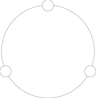
Figure 1: The Dynkin diagram of $A_{2}^{(1)}$

Note that the extended root system (3.31) has $C_{3}$ symmetry, so it is neat that it is related to $C_{3}$ symmetric monopoles. Although the planar interpretation is lost for $n>3$ the cyclic $C_{n}$ symmetry is still present for the extended root system of $A_{n-1}^{(1)}$, since the roots have a complex representation in terms of the $n$th roots of unity (see for eg [2]). The cyclic $C_{n}$ symmetry is transparent in the Dynkin diagram for $A_{n-1}^{(1)}$, which is a closed chain containing $n$ nodes. The example of $n=3$ is shown suggestively in Figure 1, to resemble three monopoles with cyclic symmetry. It would be interesting to consider the Toda lattice to monopoles correspondence for other Lie algebras, and to see whether the resulting monopoles have symmetries associated with those of the Dynkin diagram. Given the McKay correspondence [17] it is expected that the extended algebras of type A-D-E are associated to monopoles with respectively cyclic, dihedral and Platonic symmetry.

Now we have the Nahm data in terms of the Toda fields we need to compute the static quasi-periodic soliton. (Only solitons on the infinite line were studied in [10]). We can still work with the $\phi_{i}$ fields even in the imaginary coupled theory if we regard them as complex fields. Defining the field $f_{j}=e^{\phi_{j}}-1$ the static Toda field equation becomes

$$-\partial_{x}^{2}\log(1+f_{j})=f_{j+1}+f_{j-1}-2f_{j}.$$ (3.36)

The key to constructing the soliton solution is the remarkable elliptic function addition formula (which can be obtained from the one given in [26])

$$dc^{2}(u+v)+dc^{2}(u-v)-2dc^{2}(u)=-\frac{d^{2}}{du^{2}}\log(dc^{2}(u)-1-cs^{2}(v))$$ (3.37)

where all the elliptic functions have the same modulus $k$, which we suppress for clarity. Setting

$$u=x+2Kj/3+\delta,\hskip 28.45274ptv=2K/3,\hskip 28.45274ptf_{j}=dc^{2}(u)-B$$ (3.38)

the identity (3.37) is transformed into the equation (3.36) if the condition that

$$B=2+cs^{2}(2K/3)$$ (3.39)

is also satisfied. Hence the soliton solution is given by

$$f_{j}=dc^{2}(x+2jK/3+\delta)-2-cs^{2}(2K/3)$$ (3.40)

and has period $2K$ in $x$. Note that the periodicity of the lattice is satisfied $f_{j+3}=f_{j}$. In terms of the variables for the Nahm data the solution is

$$q_{j}^{2}=dc^{2}(\theta_{j})-1-cs^{2}(2K/3),\hskip 28.45274pt\mbox{where}\hskip 28.45274pt\theta_{j}=x+2jK/3+\delta.$$ (3.41)

The required periodicity in $s$ of the Nahm data can be achieved by a suitable choice of the scale $\lambda$, and the reality conditions are also satisfied. So the only condition that still needs to be met is that the Nahm data has a pole at $s=0$ whose residues define the 3-dimensional irreducible representation of $su(2)$. It is a simple task to position a pole at $s=0$ by choosing the constant $\delta=K$. Then since $dc(x+K)$ has a simple pole at $x=0$ by the above formula $q_{0}$ has a simple pole at $s=0$. Also by the above formulae it is clear that all the remaining $q_{i}$ are regular at $s=0$. Using Taylor series for the elliptic functions around $x=0$ gives that as $x\rightarrow 0$

$$q_{0}\sim\frac{1}{x},\ q_{1}\sim\frac{0}{x},\ q_{2}\sim\frac{0}{x}.$$ (3.42)

Now by equation (3.10)

$$\partial_{x}(p_{j}-p_{j+1})=q_{j}^{2}-q_{j+1}^{2}$$ (3.43)

which can be integrated to determine the pole behaviour

$$p_{0}-p_{1}\sim-\frac{1}{x},\ p_{1}-p_{2}\sim\frac{0}{x},\ p_{2}-p_{0}\sim\frac{1}{x}.$$ (3.44)

Hence at the $s=0$ pole the behaviour of the third Nahm matrix is $T_{3}\sim R_{3}/s$ where

$$R_{3}=\frac{i}{2}\mbox{diag}(1,0,-1).$$ (3.45)

Thus $\mbox{tr}R_{3}^{2}=-1/2$ which unfortunately identifies the representation formed by the matrix residues as the reducible representation $\underline{2}\oplus\underline{1}$. So the soliton generated Nahm matrices fall at the final hurdle and do not correspond to Nahm data. It is easy to see that at any pole of the soliton generated Nahm solutions only one of the $q_{i}$’s can be singular, and that this is the case for all $n$. Hence only for $n=2$ can the representation formed by the matrix residues be irreducible.

In summary, we have shown that for all $n$ the problem of solving Nahm’s equation to determine cyclic $C_{n}$ symmetric $n$-monopoles is equivalent to solving the quasi-periodic problem for the $A_{n-1}^{(1)}$ Toda lattice, but that only for the case $n=2$ does the simple soliton solution generate the Nahm data. For $n>2$ the Toda equation is still integrable, but the general solution will involve abelian integrals of genus $n-1$. The difficulty then lies in determining those solutions which satisfy the Nahm data conditions, which appears a highly non-trivial exercise.

4 Conclusion

In this note we have observed that the Seiberg-Witten curves, which are known to be equivalent to the spectral curves of the Toda lattice, can be related to the spectral curves of BPS monopoles. The implied connection between Toda theory and monopoles has been made explicit via the ADHMN construction and in the simplest case of two monopoles it has been shown that the affine Toda soliton generates the known 2-monopole solution.

Perhaps the observations in this note are no more than a curiosity, but there are a couple of speculative possibilities which could be pursued. The first is that the moduli space of a given Seiberg-Witten curve has singular points at which massless monopoles appear in the supersymmetric Yang-Mills theory. It has recently been shown [13, 25] that there are certain singular points in the classical BPS moduli space where the classical monopole solution developes additional spurious zeros of the Higgs field. Given the identification discussed in this note then perhaps there could be some connection between these two phenomena. Secondly, through the Toda lattice connection it was shown [5] that the special Seiberg-Witten differential emerges in the study of the Whitham dynamics of the Toda lattice, which essentially involves constructing a dynamics on the moduli space of the spectral curves. Hence is there a similar interpretation of the differential in terms of a dynamics on the monopole moduli space, and if so could the classical monopole moduli space metric play a role in $N=2$ SUSY duality as it does in S-duality in the corresponding $N=4$ SUSY theory [23].

Acknowledgements

Many thanks to Nigel Hitchin for useful comments.

References

- [1] M.F. Atiyah and N.J. Hitchin, ‘The geometry and dynamics of magnetic monopoles’, Princeton University Press, 1988.
- [2] H.W. Braden, E. Corrigan, P.E. Dorey and R. Sasaki, Nucl. Phys. B338, 689 (1990).
- [3] A.S. Dancer, Nonlinearity 5, 1355 (1992).
- [4] A. Erdm\a’elyi, Higher Transcendental Functions (Bateman Project) vol 3 (New York: McGraw-Hill).
- [5] A. Gorskii, I. Krichever, A. Marshakov, A. Mironov and A. Morozov, Phys. Lett. B355, 466 (1995).
- [6] N.J. Hitchin, Commun. Math. Phys. 83, 579 (1982).
- [7] N.J. Hitchin, Commun. Math. Phys. 89, 145 (1983).
- [8] N.J. Hitchin, N.S. Manton and M.K. Murray, Nonlinearity, 8, 661 (1995).
- [9] N.J. Hitchin and M.K. Murray, Commun. Math. Phys. 114, 463 (1988).
- [10] T.J. Hollowood, Nucl. Phys. B384, 523 (1992).
- [11] C.J. Houghton and P.M. Sutcliffe, in preparation.
- [12] C.J. Houghton and P.M. Sutcliffe, ‘Inversion symmetric 3-monopoles and the Atiyah-Hitchin manifold’, preprint DAMTP 96-32, UKC/IMS/96-24.
- [13] C.J. Houghton and P.M. Sutcliffe, Nucl. Phys. B464, 59 (1996).
- [14] J.Hurtubise and M.K. Murray, Commun. Math. Phys. 122, 35 (1989).
- [15] A. Klemm, W. Lerche, S. Yankielowicz and S. Theisen, Phys. Lett. B344, 169 (1995).
- [16] E.J. Martinec and N.P. Warner, Nucl. Phys. B459, 97 (1996).
- [17] J. McKay, Proc. Sympos. Pure Math. 37, 183 (1980).
- [18] W. Nahm, ‘The construction of all self-dual multimonopoles by the ADHM method’, in Monopoles in quantum field theory, eds. N.S. Craigie, P. Goddard and W. Nahm, World Scientific, 1982.
- [19] H. Nakajima, ‘Monopoles and Nahm’s equation’, talk presented at the British Mathematical Colloquium, UMIST, 1996.
- [20] D.I. Olive and N. Turok, Nucl. Phys. B220[FS8], 491 (1983).
- [21] P.D. Parmentier, in Solitons in Action, eds. K. Lonngren and A. Scott, New York Academic, 1978.
- [22] N. Seiberg and E. Witten, Nucl. Phys. B246, 19 (1994). Erratum-ibid B430, 485 (1994).
- [23] A. Sen, Phys. Lett. B329, 217 (1994).
- [24] P.M. Sutcliffe, Nonlinearity 8, 411 (1995).
- [25] P.M. Sutcliffe, ‘Monopole zeros’, to appear in Phys. Lett. B.
- [26] M.Toda, ‘Nonlinear waves and Solitons’, Kluwer Academic Publishers, 1989.
- [27] R.S. Ward, Phys. Lett. A112, 3 (1985).