TIT/HEP–333

March 1996

FRACTAL STRUCTURE OF SPACE–TIME IN TWO-DIMENSIONAL QUANTUM GRAVITY 

We show that universal functions play an important role in the observation of the fractal structure of space–time in the numerical simulation of quantum gravity.

1 Introduction

The fractal structure of space–time is one of the most interesting aspects in quantum gravity. Since we know well-defined theories of quantum gravity only in two dimensions, we here confine ourselves to the two-dimensional quantum gravity. We study the fractal structure of space–time from the points of view of the geodesic distance as well as the “time” in the diffusion equation.

The partition function for the two-dimensional quantum gravity is

$$Z_{V}\ =\ \int\!\!\!\int\!\frac{{\cal D}[g_{ab}]{\cal D}\phi}{\rm Vol(Diff)}\,\delta(\int\!\!\!\sqrt{g}-V)\,e^{-S_{\rm matter}[g,\phi]}\,,$$ (1)

where $\phi$ symbolizes matter fields. We have here fixed the volume of space–time $V=\int\!\!\sqrt{g}$ by $\delta$-function. The usual cosmological term $\Lambda\!\int\!\!\sqrt{g}$ is recovered by the Laplace transformation: $Z_{\Lambda}=\int_{0}^{\infty}\!\!dVe^{-\Lambda V}Z_{V}$.

1.1 Geodesic distance

We first study the fractal structure by using the geodesic distance. Let us consider the total length of the boundaries $S_{V}(R)$, which are separated from a given point with a geodesic distance $R$. The average of $S_{V}(R)$ is given by

$$\left\langle S_{V}(R)\right\rangle\ =\ \frac{G_{V}(R)}{VZ_{V}}\,,$$ (2)

where $G_{V}(R)$ is the two-point function defined by $\!{}^{{\bf?}}$

$$G_{V}(R) = \int\!\!\!\int\!\frac{{\cal D}[g_{ab}]{\cal D}\phi}{\rm Vol(Diff)}\,\delta(\int\!\!\!\sqrt{g}-V)\,e^{-S_{\rm matter}[g,\phi]}$$

$$\times\int\!\!\!\int\!d^{2}\xi\sqrt{g(\xi)}d^{2}\xi_{0}\sqrt{g(\xi_{0})}\,\delta(d_{g}(\xi,\xi_{0})-R)\,.$$

$d_{g}(\xi,\xi_{0})$ denotes the geodesic distance between two points labeled by $\xi$ and $\xi_{0}$. Since $dR\left\langle S_{V}(R)\right\rangle$ is a unit volume, we have

$$\int_{0}^{\infty}\!\!\!dR\left\langle S_{V}(R)\right\rangle\ =\ V\,.$$ (4)

According to the scaling arguments, the following generic behavior is derived:

$$\left\langle S_{V}(R)\right\rangle\ =\ V^{1-\nu}\,U(X)~{}~{}~{}~{}~{}\hbox{with}~{}~{}X\,=\,\frac{R}{V^{\nu}}\,.$$ (5)

Here a parameter $\nu$ is introduced so as to let $X=R/V^{\nu}$ be dimensionless.

Expanding (5) around $R\sim 0$, a kind of fractal structure is expected, i.e.,

$$\left\langle S_{V}(R)\right\rangle\ \sim\ {\rm const.}\,V^{1-\nu d_{h}}R^{d_{h}-1}~{}~{}~{}~{}{\rm for}~{}~{}R\sim 0\,,$$ (6)

which defines the intrinsic Hausdorff dimension $d_{h}$. For a smooth $d$-dimensional manifold we have $1/\nu=d_{h}=d$. If $\left\langle S_{V=\infty}(R)\right\rangle$ is non-zero finite, i.e.,

$$\nu\,d_{h}\,=\,1\,,$$ (7)

a kind of “flat” fractal space is realized when $V\to\infty$. We call the fractal which becomes a “flat” fractal space for $V\to\infty$ by the “smooth” fractal.

We will show later that the function $U(X)$ introduced in (5) plays an important role in numerical simulation. From (5) and (6) we obtain

$$U(X)\ =\ V^{\nu-1}\left\langle S_{V}(R)\right\rangle\ =\ X^{d_{h}-1}F(X)\,,$$ (8)

where $F(0)$ is non-zero finite. From (4) we find that $U(X)$ is normalized as

$$\int_{0}^{\infty}\!\!dX\,U(X)\ =\ 1\,.$$ (9)

In the case of pure quantum gravity, one can calculate $G_{V}(R)$ analytically $\!{}^{{\bf?}}$ using the transfer matrix formalism $\!{}^{{\bf?}}$: (See also the appendix in ref. $\!{}^{{\bf?}}$)

$$G_{V}(R)\ =\ 12\sqrt{\pi}A\int_{\sigma-i\infty}^{\sigma+i\infty}\!\frac{d\Lambda}{2\pi i}\,e^{\Lambda V}\Lambda^{3/4}\;\frac{\cosh\Lambda^{1/4}R}{\sinh^{3}\Lambda^{1/4}R}\,,$$ (10)

while $Z_{V}=A/V^{7/2}$, where $A$ is constant. Using (2) and (10), we find

$$\left\langle S_{V}(R)\right\rangle\ \sim\ {\rm const.}\,R^{3}~{}~{}~{}~{}{\rm for}~{}~{}R\sim 0\,.$$ (11)

Thus, we find $1/\nu=d_{h}=4$ in pure gravity. Note that the “smooth” fractal condition (7) is satisfied in this case.

1.2 Time of Diffusion

Now, let us introduce the “time” of diffusion in order to analyze another aspect of fractal structure. The diffusion equation has the form,

$$\frac{\partial}{\partial T}K_{g}(\xi,\xi_{0};T)\ =\ \Delta_{g}K_{g}(\xi,\xi_{0};T)\,.$$ (12)

We here consider the following initial condition,

$$K_{g}(\xi,\xi_{0};0)\ =\ \frac{1}{\sqrt{g(\xi)}}\,\delta(\xi-\xi_{0})\,.$$ (13)

$K_{g}(\xi,\xi_{0};T)$ is the probability of diffused matter per unit volume at coordinate $\xi$ at time $T$. We introduce the following wave function $\bar{K}_{V}(R;T)$, which is the average of $K_{g}(\xi,\xi_{0};T)$ with a fixed geodesic distance $R$:

$$\bar{K}_{V}(R;T) = \frac{1}{G_{V}(R)}\int\!\!\!\int\!\frac{{\cal D}[g_{ab}]{\cal D}\phi}{\rm Vol(Diff)}\,\delta(\int\!\!\!\sqrt{g}-V)\,e^{-S_{\rm matter}[g,\phi]}$$

$$\times\int\!\!\!\int\!d^{2}\xi\sqrt{g(\xi)}d^{2}\xi_{0}\sqrt{g(\xi_{0})}\,\delta(d_{g}(\xi,\xi_{0})-R)\,K_{g}(\xi,\xi_{0};T)\,.$$

Since $\bar{K}_{V}(R;T)$ satisfies

$$\int_{0}^{\infty}\!\!\!dR\left\langle S_{V}(R)\right\rangle\bar{K}_{V}(R;T)\ =\ 1\,,$$ (15)

the scaling arguments lead to

$$\bar{K}_{V}(R;T)\ =\ \frac{1}{V}\,P(X;Y)~{}~{}~{}~{}~{}\hbox{with}~{}~{}X\,=\,\frac{R}{V^{\nu}}\,,~{}~{}~{}Y\,=\,\frac{T}{V^{\lambda}}\,,$$ (16)

where a parameter $\lambda$ is introduced so as to let $Y=T/V^{\lambda}$ be dimensionless. Similarly to (9), we find

$$\int_{0}^{\infty}\!\!dX\,U(X)\,P(X;Y)\ =\ 1\,.$$ (17)

Thus, $P(X;Y)$ as well as $U(X)$ are considered as a kind of universal functions.

Now we consider $\bar{K}_{V}(0;T)$ which is the average of the return probability of diffused matter at time $T$. Around $T\sim 0$, $\bar{K}_{V}(0;T)$ will be

$$\bar{K}_{V}(0;T)\ \sim\ {\rm const.}\,\frac{V^{\lambda d_{s}/2-1}}{T^{d_{s}/2}}~{}~{}~{}~{}{\rm for}~{}~{}~{}T\sim 0\,,$$ (18)

which defines the spectral dimension $d_{s}$. We also consider the average geodesic distance travel by diffusion over time $T$,

$$\left\langle R_{V}(T)\right\rangle\stackrel{{\scriptstyle\rm def}}{{\equiv}}\int_{0}^{\infty}\!\!\!dR\left\langle S_{V}(R)\right\rangle R\,\bar{K}_{V}(R;T)\ \sim\ {\rm const.}\,V^{\nu-\lambda\sigma}\,T^{\sigma}~{}~{}~{}~{}{\rm for}~{}~{}~{}T\sim 0\,.$$ (19)

For a smooth $d$-dimensional manifold we have $2/\lambda=d_{s}=d$ and $\sigma=1/2$. If the surface is a “smooth” fractal, the right-hand sides of (18) and (19) take non-zero finite values for $V\to\infty$. Then we find

$$\lambda d_{s}\,=\,2\,,~{}~{}~{}\lambda\sigma\,=\,\nu\,,$$ (20)

as “smooth” fractal conditions. The universal functions for (18) and (19) are $P(0;Y)=V\bar{K}_{V}(0;T)$ and $\int_{0}^{\infty}dXU(X)XP(X;Y)=V^{-\nu}\left\langle R_{V}(T)\right\rangle$, respectively.

2 Numerical Simulation

The setup of the numerical simulations in ref $\!{}^{{\bf?}}$ is as follows: We use the dynamical triangulation, i.e., ensembles of surfaces built of equilateral triangles with spherical topology and a fixed number of triangles. These surfaces can be viewed as dual to planar $\phi^{3}$ diagrams. In the language of the $\phi^{3}$ theory, we include diagrams containing tadpole and self-energy subdiagrams. In simulation both the standard flips and the new global moves (minbu surgery) are organized. The new move helps to reduce the correlation times $\!{}^{{\bf?},{\bf?},{\bf?},{\bf?}}$. We study various sizes of systems with 1000, 2000, 4000, 8000, 16000 and 32000 triangles. In the analysis of the diffusion equation only triangulation with 4000 and 16000 triangles are used because of the large measurement times.

2.1 Geodesic distance

In the dynamical triangulation the volume $V$ is identified with the number of triangles $N$, while the geodesic distance $R$ is done with the number of dual links $r$ of geodesic curve defined as the shortest path on dual link between two triangles. Introducing the lattice spacing parameter $\varepsilon$, one can write

$$V\ =\ N\,\varepsilon^{2}\,,~{}~{}~{}~{}~{}~{}~{}R\ =\ \alpha\,r\,\varepsilon^{2\nu}\,,$$ (21)

where $\alpha$ is a dimensionless constant parameter. The parameter $\nu$ is introduced again because $X=R/V^{\nu}$ is dimensionless.

Let $S_{N}(r)$ be the number of triangles on the boundaries which can be reached from a given triangle with the geodesic distance $r$. The average of $S_{N}(r)$ under the dynamical triangulation, $\left\langle S_{N}(r)\right\rangle$, can be considered as a unit volume with the direction of $r$ on fractal surface, and then satisfies

$$\sum_{r=0}^{\infty}\left\langle S_{N}(r)\right\rangle\ =\ N\,.$$ (22)

The discrete version of $U(X)$ is

$$u(x)\ =\ N^{\nu-1}\left\langle S_{N}(r)\right\rangle\ =\ x^{d_{h}-1}f(x)~{}~{}~{}~{}~{}\hbox{with}~{}~{}x\ =\ \frac{r}{N^{\nu}}\,,$$ (23)

where $f(0)$ is non-zero finite. $u(x)$ and $x$ are related with $U(X)$ and $X$ as

$$u(x)\ =\ \alpha\,U(X)\,,~{}~{}~{}~{}~{}~{}~{}~{}\alpha\,x\ =\ X\,.$$ (24)

By choosing a reasonable value of $\nu$, the same function $u(x)$ is expected for any size of systems. Thus, one can determine the value of $\nu$ from the point of view of finite size scaling. One can also determine the value of $d_{h}$ by

$$\frac{d\log u(x)}{d\log x}\ =\ d_{h}-1+{\rm const.}\,x^{k}+o(x^{k})\,.$$ (25)

In refs. $\!{}^{{\bf?},{\bf?}}$, $d\log\left\langle S_{N}(r)\right\rangle/d\log r$ for large $N$ is studied by numerical simulation. In ref. $\!{}^{{\bf?}}$ the authors have succeeded in observing the scaling law for $c=-2$ model by using quite a lot of triangles (five million triangles). We will show that the universal function $u(x)$ helps us much more effectively to observe the fractal structure in numerical simulations.

Pure gravity

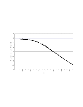
Pure gravity is a good test case for numerical simulations because we know the exact formula for $G_{V}(R)$ in (10), the value of $\nu=1/4$ and $\alpha=\sqrt{6/(12+13\sqrt{3})}$, and consequently the exact expression for $u(x)$. Comparing the numerical data with the analytic curve, we find that a much better result is obtained by using a “phenomenological” variable $x$,

$$x\ =\ \frac{r+a}{N^{\nu}+b}\,,$$ (26)

instead of $x=r/N^{\nu}$. This shift is reasonable from the point of view of lattice artifacts.

In fig. 1 we show the data as well as the theoretical curve of $u(x)$ with an optimal choice of $a$ and $b$. The agreement is almost perfect and the conclusion is that we already see continuum physics for systems as small as 1000 triangles in the case of pure gravity if we include simple finite size corrections like (26).

Figure 1: $u(x)$ as well as $d\log u(x)/d\log x$ for pure gravity with system sizes 1K, 2K, 4K, …, 32K triangles as a function of the scaled variable $x=(r+5.5)/(N^{1/4}-0.45)$. The theoretical distribution (the fully drawn line) is also displayed.

Gravity coupled to matter

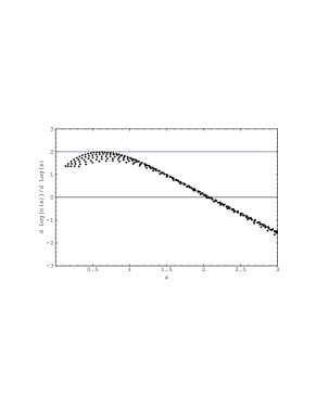
We can now perform the analysis outlined above in the case of gravity coupled to matter: Ising spins coupled to gravity ($c=1/2$), three-state Potts model coupled to gravity ($c=4/5$) and one to five Gaussian fields coupled to gravity ($c=1,\ldots,5$). The matter fields are placed in the centers of triangles. In these cases we do not know the theoretical values of $\nu$ and $d_{h}$.

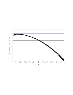
For all these theories we measure $u(x)$ and try to determine the values of $\nu$ and $d_{h}$ according to (23), (25) and (26). We illustrate $u(x)$ and $d\log u(x)/d\log x$ for $c=1/2$, $1$, $2$ and $c=5$ in fig. 2. Each of the graphs contains the scaled data for system sizes 1000, 2000, 4000, 8000, 16000 and 32000 triangles. The results for other models ($c=4/5$, $3$ and $4$) are similar. If $\nu$ is chosen to be $1/4$ for $c\leq 1$, $1/3$ for $c=2$ and $1/2$ for $c=5$, respectively, we see as good scaling as in the case of pure gravity. For $c\leq 1$ the best values of the constants $a$ and $b$ in (26) are very close to the pure gravity values. The result of $1/\nu$ is shown on the left in fig. 3. From the right in fig. 2 we find that the “smooth” fractal condition (7) is almost perfectly satisfied for all these theories. We have also checked that the exponent $k$ defined in (25) has the value, $k\sim 4$ for $c\leq 1$ while $k\sim 2$ for $c=4$ and $5$.

Figure 2: $u(x)$ as well as $d\log u(x)/d\log x$ for $c=1/2$, $1$, $2$ and $5$. We have assumed $\nu=1/4$ for $c=1/2$ and $c=1$, $\nu=1/3$ for $c=2$ and $\nu=1/2$ for $c=5$. The constants $a,b$ determined this way are quite close to the pure gravity values for $c=1/2$ and $c=1$. In all cases the data include the following discretized volume sizes: $N=$ 1K, 2K, 4K, …, 32K.

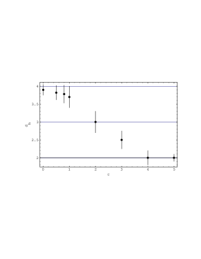
We get the string susceptibility $\gamma_{s}$ easily by the benefit of the minbu surgery algorithm. On the right in fig. 3 we show the measured $\gamma_{s}$ for various theories. Both figures in fig. 3 corroborates on the idea that 2D quantum gravity with large $c$ is the branched polymer model which has $1/\nu=d_{h}=2$ and $\gamma_{s}=1/2$.

Figure 3: The left figure shows $1/\nu~{}(\approx d_{h})$ determined by finite size scaling for $c=0$, $1/2$, $4/5$, $1$, $2$, $3$, $4$, and $5$. The dots denote the best values of $1/\nu~{}(\approx d_{h})$. The right figure shows the measured string susceptibility $\gamma_{s}$ versus central charge $c$. We here assume $Z_{V}={\rm const.}\,V^{\gamma_{s}-3}$. This is the reason why the measured $\gamma_{s}$ for $c=1$ disagrees with the theoretical value.

2.2 Time of Diffusion

We now turn to the measurement of the spectral dimension $d_{s}$ introduced in (18) and (19). The diffusion equation at the discrete level describes a random walk. We denotes the discrete version of $\bar{K}_{V}(R;T)$ by $\bar{k}_{N}(r;t)$. $t$ is the number of step of random walk, which is related with $T$ as

$$T\ =\ \beta\,t\,\varepsilon^{2\lambda}\,,$$ (27)

where $\beta$ is a dimensionless constant parameter. Since $\bar{k}_{N}(r;t)$ satisfies

$$\sum_{r=0}^{\infty}\left\langle S_{N}(r)\right\rangle\bar{k}_{N}(r;t)\ =\ 1\,,$$ (28)

the discrete version of (16) is

$$\bar{k}_{N}(r;t)\ =\ \frac{1}{N}\,p(x;y)~{}~{}~{}~{}~{}\hbox{with}~{}~{}x\,=\,\frac{r}{N^{\nu}}\,,~{}~{}~{}y\,=\,\frac{t}{N^{\lambda}}\,.$$ (29)

$p(x;y)$ is related with $P(X;Y)$ as

$$p(x;y)\ =\ P(X;Y)\,,~{}~{}~{}~{}~{}~{}~{}~{}\beta\,y\ =\ Y\,.$$ (30)

The return probability of random walk is

$$\bar{k}_{N}(0;t)\ \sim\ {\rm const.}\,\frac{N^{\lambda d_{s}/2-1}}{t^{d_{s}/2}}~{}~{}~{}~{}{\rm for}~{}~{}~{}t\sim 0\,,$$ (31)

while the average geodesic distance travel by random walk over time $t$ is

$$\left\langle r_{N}(t)\right\rangle\ \stackrel{{\scriptstyle\rm def}}{{\equiv}}\ \sum_{r=0}^{\infty}\left\langle S_{N}(r)\right\rangle r\,\bar{k}_{N}(r;t)\ \sim\ {\rm const.}\,N^{\nu-\lambda\sigma}\,t^{\sigma}~{}~{}~{}~{}{\rm for}~{}~{}~{}t\sim 0\,.$$ (32)

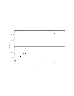
In fig. 4 we show $-2d\log\bar{k}_{N}(0;t)/d\log t~{}(\approx d_{s})$ and $\left\langle r_{N}(t)\right\rangle^{4}$ as a function of time for $c=0$ (pure gravity), $1/2$, $1$, $3$, $5$. From the left in fig. 4 we observe that $d_{s}$ is consistent with 2 for $c\leq 1$ and that it decreases for $c>1$. From the right figure we observe that $\sigma\approx 1/4$. We then obtain $d_{h}\approx 2d_{s}$ if the “smooth” fractal condition (20) is satisfied.

Figure 4: The left figure shows $-2d\log\bar{k}_{N}(0;t)/d\log t$ versus $t$ for $c=0$ (top curve), $c=1/2$, $c=1$, $c=3$ and $c=5$ (bottom curve). The system size is $N=$ 16K. The right figure shows $\left\langle r_{N}(t)\right\rangle^{4}$ versus $t$ for $c=0$ (bottom curve), $c=1$, $c=3$ and $c=5$ (top curve). The system size is $N=$ 4K. Straight lines (as observed) indicate $\sigma=1/4$ according to (32)

3 Discussion

We generalize the definition of the two-point function in (1.1) as follows: Let $\Psi_{g}(\xi,\xi_{0};M_{i})$ be an observable which depends on two coordinates $\xi$ and $\xi_{0}$ as well as the metric, where $M_{i}$ symbolizes some parameters. We define the average of $\Psi_{g}(\xi,\xi_{0};M_{i})$ with a fixed geodesic distance $R$ as

$${\overline{\Psi}\hskip 1.0pt{}}_{V}(R;M_{i}) \stackrel{{\scriptstyle\rm def}}{{\equiv}} \frac{1}{G_{V}(R)}\int\!\!\!\int\!\frac{{\cal D}[g_{ab}]{\cal D}\phi}{\rm Vol(Diff)}\,\delta(\int\!\!\!\sqrt{g}-V)\,e^{-S_{\rm matter}[g,\phi]}$$

$$\times\int\!\!\!\int\!d^{2}\xi\sqrt{g(\xi)}d^{2}\xi_{0}\sqrt{g(\xi_{0})}\,\delta(d_{g}(\xi,\xi_{0})-R)\,\Psi_{g}(\xi,\xi_{0};M_{i})\,.$$

Note that ${\overline{\Psi}\hskip 1.0pt{}}_{V}(R;M_{i})$ satisfies

$$\int_{0}^{\infty}\!\!\!dR\left\langle S_{V}(R)\right\rangle{\overline{\Psi}\hskip 1.0pt{}}_{V}(R;M_{i})\ =\ \frac{\left\langle\Psi(M_{i})\right\rangle_{V}}{V}\,,$$ (34)

where

$$\left\langle\Psi(M_{i})\right\rangle_{V} = \frac{1}{Z_{V}}\int\!\!\!\int\!\frac{{\cal D}[g_{ab}]{\cal D}\phi}{\rm Vol(Diff)}\,\delta(\int\!\!\!\sqrt{g}-V)\,e^{-S_{\rm matter}[g,\phi]}$$

$$\times\int\!\!\!\int\!d^{2}\xi\sqrt{g(\xi)}d^{2}\xi_{0}\sqrt{g(\xi_{0})}\,\Psi_{g}(\xi,\xi_{0};M_{i})\,.$$

If $\left\langle\Psi(M_{i})\right\rangle_{V}\neq 0$, one can define a universal function,

$$Q(X;Y_{i})\ =\ \frac{V^{2}}{\left\langle\Psi(M_{i})\right\rangle_{V}}\,{\overline{\Psi}\hskip 1.0pt{}}_{V}(R;M_{i})~{}~{}~{}~{}~{}\hbox{with}~{}~{}X\,=\,\frac{R}{V^{\nu}}\,,~{}~{}~{}Y_{i}\,=\,\frac{M_{i}}{V^{\mu_{i}}}\,,$$ (36)

where a parameter $\mu_{i}$ makes $Y_{i}=M_{i}/V^{\mu_{i}}$ dimensionless. Similarly to (9) and (17), we find

$$\int_{0}^{\infty}\!\!dX\,U(X)\,Q(X;Y_{i})\ =\ 1\,.$$ (37)

The universal function of the moment like (19) is in general expressed as

$$\int_{0}^{\infty}\!\!dX\,U(X)\,f(X;Y_{i})\,Q(X;Y_{i})\,,$$ (38)

which is obtained by multiplying $f(d_{g}(\xi,\xi_{0});M_{i})$ in front of $\Psi_{g}$ in (3). It is straightforward to obtain the discrete version of (36), (37) and (38).

We have several examples as follows: i) $\Psi_{g}=1$ is a trivial case because $Q(X)=1$. ii) $\Psi_{g}=K_{g}(\xi,\xi_{0};T)$ is already discussed in section (1.2), i.e., $Q(X;Y)=P(X;Y)$. iii) $\Psi_{g}=\phi_{1}(\xi)\phi_{2}(\xi_{0})$ leads to $Q(X)=V^{\Delta_{1}+\Delta_{2}}{\overline{\Psi}\hskip 1.0pt{}}_{V}(R)$, where $\Delta_{i}$ is defined by $\left\langle\int\!\!\sqrt{g}\phi_{i}\right\rangle_{V}\propto V^{1-\Delta_{i}}$. If the surface is a “smooth” fractal, one can expect ${\overline{\Psi}\hskip 1.0pt{}}_{V}(R)\sim{\rm const.}\,R^{-(\Delta_{1}+\Delta_{2})/\nu}$ for $R\sim 0$.

References

- [1] J. Ambjørn and Y. Watabiki, Nucl. Phys. B 445, 129 (1995).
- [2] J. Ambjørn, J. Jurkiewicz and Y. Watabiki, Nucl. Phys. B 454, 313 (1995).
- [3] J. Ambjørn, B. Durhuus and T. Jonsson, Phys. Lett. B 244, 403 (1990).
- [4] Y. Watabiki, Prog. Theor. Phys. Suppl. No. 114, 1 (1993).
- [5] H. Kawai, N. Kawamoto, T. Mogami and Y. Watabiki, Phys. Lett. B 306, 19 (1993).
- [6] J. Ambjørn, P. Bialas, J. Jurkiewicz, Z. Burda and B. Petersson, Phys. Lett. B 325, 337 (1994).
- [7] J. Ambjørn and J. Jurkiewicz, Nucl. Phys. B 451, 643 (1995).
- [8] S. Jain and S. Mathur, Phys. Lett. B 286, 239 (1992).
- [9] J. Ambjørn, S. Jain and G. Thorleifsson, Phys. Lett. B 307, 34 (1993); J. Ambjørn, G. Thorleifsson, Phys. Lett. B 323, 7 (1994).
- [10] S. Catterall, G. Thorleifsson, M. Bowick and V. John, Phys. Lett. B 354, 58 (1995).
- [11] M.E. Agishtein and A.A. Migdal, Int. J. Mod. Phys. C 1, 165 (1990); Nucl. Phys. B 350, 690 (1991).
- [12] N. Kawamoto, V.A. Kazakov, Y. Saeki and Y. Watabiki, Phys. Rev. Lett. 68, 2113 (1992); Nucl. Phys. B (Proc. Suppl.) 26, 584 (1992).