CTP-2536 Imperial/TP/95-96/50 PUPT-1624 hep-th/9605169
The Ising model with a boundary magnetic field
on a random surface

Abstract

The bulk and boundary magnetizations are calculated for the critical Ising model on a randomly triangulated disk in the presence of a boundary magnetic field $h$. In the continuum limit this model corresponds to a $c=1/2$ conformal field theory coupled to 2D quantum gravity, with a boundary term breaking conformal invariance. It is found that as $h$ increases, the average magnetization of a bulk spin decreases, an effect that is explained in terms of fluctuations of the geometry. By introducing an $h$-dependent rescaling factor, the disk partition function and bulk magnetization can be expressed as functions of an effective boundary length and bulk area with no further dependence on $h$, except that the bulk magnetization is discontinuous and vanishes at $h=0$. These results suggest that just as in flat space, the boundary field generates a renormalization group flow towards $h=\infty$. An exact analytic expression for the boundary magnetization as a function of $h$ is linear near $h=0$, leading to a finite nonzero magnetic susceptibility at the critical temperature.

The Ising model with a boundary magnetic field[5] has been of renewed interest recently as a simple example of a two-dimensional integrable field theory with nontrivial boundary interactions [6, 7, 8]. The only boundary conditions for the Ising model which preserve conformal invariance[9] are free boundary conditions (where the boundary field $h$ vanishes), and fixed spin boundary conditions (where $h=\pm\infty$). Putting an arbitrary field $h$ on the boundary generates a renormalization group (RG) flow which goes away from the free boundary condition towards the fixed boundary condition [10].

Another subject of recent interest has been the effect of different boundary conditions in string theory[11]. Just as there are two types of conformally invariant boundary conditions for the Ising theory, a conformal field theory of a single bosonic field can have two conformally invariant boundary conditions: Neumann and Dirichlet. By considering the continuum limit of the Ising model as a single free fermion, in the context of superconformal field theory it can be shown that boundary conditions in these two models are related by supersymmetry, with Neumann corresponding to free Ising spins and Dirichlet corresponding to fixed spins.

In this letter we consider the effect of a boundary magnetic field on the Ising model on a random surface (the noncritical string with $c=1/2$). This theory describes a single Ising spin (or equivalently a free fermion) coupled to 2D quantum gravity. The Ising model on a random surface can be studied in several ways. One approach is to use the continuum formulation of noncritical string theory as a conformal field theory coupled to a Liouville field[12, 13]. Another approach is to describe the model as a matrix model, involving a sum over discrete surfaces[14]; in the discrete formalism, a continuum limit can be taken by tuning coupling constants until the surfaces become arbitrarily large; in this limit the theory corresponds to the continuous Liouville theory. In this work we will use a discrete formulation of the Ising model on a random surface; to calculate correlation functions in this theory we use the method of discrete loop equations developed in two previous papers [15, 16]. Similar methods were discussed in[17, 18].

We present here only the results of our investigation. The details of the calculations, which are algebraically tedious, will be presented in a later publication.

In the discrete formulation, the Ising model on a random surface of disk topology has a partition function which is given by a sum over all possible triangulations of the disk. For each triangulation, the Boltzmann weight is given by placing a single Ising spin on each triangle, and summing over all possible spin configurations, giving the Ising partition function on that particular geometry. This model can be written as a matrix model[14]

$${\cal Z}(g,c)=\int{\rm D}U\;{\rm D}V\;\exp\left(-NS(U,V)\right)\ ,$$ (1)

with

$$S(U,V)={\rm Tr}\left[\frac{1}{2}(U^{2}+V^{2})-cUV-\frac{g}{3}(U^{3}+V^{3})\right]\,,$$ (2)

where $U$ and $V$ are $N\times N$ hermitian matrices.

The first calculation we wish to consider is that of the disk amplitude when the spins on the boundary are subjected to an external magnetic field $h$. In the matrix model language, dropping all factors of $N$ as we work in the large $N$ limit, we wish to compute

$$\phi(h,x,g,c)=\sum_{k=0}^{\infty}x^{k}\langle{\rm Tr}\;(e^{h}U+e^{-h}V)^{k}\rangle\equiv\sum_{k=0}^{\infty}x^{k}p_{k}\ ,$$ (3)

where $p_{k}=\langle{\rm Tr}\;(e^{h}U+e^{-h}V)^{k}\rangle$ is the amplitude for a disk with $k$ boundary spins subject to the boundary field $h$. A method for calculating such amplitudes was described in[15]. This yields a quartic equation satisfied by $\phi$, in which the coefficients are functions of $g,c,h,x,$ and $p_{i}$ with $i<4$. We omit this equation for space considerations.

The quartic equation for $\phi$ gives an exact algebraic solution for the disk partition function of the discrete theory. To find the solution in the continuum limit, we must find the critical values for $x$ and $g$ at which $\phi$ approaches a singular point. The Ising model is critical for the coupling $c_{c}=(-1+2\sqrt{7})/27$. The critical value for $g$ is known to be [14] $g_{c}=\sqrt{10c_{c}^{3}}$. After an analysis of the critical behavior of $\phi$, we find

$$x_{c}=\frac{g_{c}(1+2\sqrt{7})e^{h}}{e^{-2h}+(\sqrt{7}-1)+e^{2h}(2+\sqrt{7})}\ .$$ (4)

This expression is only valid for $h\geq 0$; $x_{c}$ is nonanalytic at $h=0$. Throughout the remainder of this letter we will restrict attention to the case $h\geq 0$; related expressions arise when $h<0$.

To take the continuum limit, we expand around the critical values $g=g_{c}e^{-\epsilon^{2}t}$, $x=x_{c}e^{-\epsilon z}$. Expanding $\phi$ in $\epsilon$, we find

$$\phi=\phi_{a}(z,t,\epsilon)+\frac{\epsilon^{4/3}}{5\cdot 2^{7/3}\alpha(h)}\Phi(Z,T)+{\cal O}(\epsilon^{5/3})\ ,$$ (5)

where $\phi_{a}$ is analytic in $\epsilon$. The second term is nonanalytic and describes the behavior in the continuum limit. Here

$$\Phi\equiv\left(Z+\sqrt{Z^{2}-4T}\right)^{4/3}+\left(Z-\sqrt{Z^{2}-4T}\right)^{4/3}\ ,$$ (6)

$t$ is rescaled by a constant factor $t=T/5$, and $z$ is rescaled by an $h$-dependent factor, $z=\alpha(h)Z$ where for $h>0$

$$\alpha(h)=\frac{(1+e^{2h})}{e^{-2h}+(-1+\sqrt{7})+e^{2h}(2+\sqrt{7})}\ .$$ (7)

At $h=0$, the scaling factor $\alpha$ is discontinuous and goes to $\alpha(0)=1/(\sqrt{2}+\sqrt{14})$; the constant factor in the universal term in (5) also changes discontinuously at this point. Note that the specific form (7) for $\alpha$ depends upon the discretization we have chosen for random surfaces.

The universal term in (5) can be converted into the asymptotic form of the disk amplitude $\tilde{\phi}(l,a)$ for fixed boundary length $l$ and disk area $a$. These forms of the amplitude are related through a Laplace transform

$$\phi_{(4/3)}(z,t)=\int{\rm d}l\int{\rm d}a\;\;e^{-zl-ta}\tilde{\phi}(l,a)\ .$$ (8)

Inverting the Laplace transform, we have

$$\tilde{\phi}={1\over 25\sqrt{3}\pi}L^{1/3}A^{-7/3}e^{-L^{2}/A}\ ,$$ (9)

with the rescalings $L=\alpha(h)l$, $A={a/5}$. Up to an irrelevant multiplicative constant, this is precisely the form of the disk amplitude when the boundary conditions are conformal [19, 17, 20, 16] (i.e., with $h=0$ or $h=\pm\infty$); however, the boundary length $l$ is rescaled by the factor $\alpha(h)$ which depends on the boundary magnetic field.

The boundary magnetization for a spin on the boundary of a disk with $k$ boundary edges and $n$ triangles is given by

$$\langle m\rangle={\langle{\rm Tr}(e^{h}U-e^{-h}V)(e^{h}U+e^{-h}V)^{k-1}\rangle_{n}\over\langle{\rm Tr}(e^{h}U+e^{-h}V)^{k}\rangle_{n}}\ ,$$ (10)

where by $\langle\rangle_{n}$ we indicate a sum over triangulations restricted to geometries with $n$ spins (the coefficient of $g^{n}$ in an expansion in $g$). We therefore look at the expectation value of the spin at a marked point on the boundary, that is

$$\psi=\sum_{k=0}^{\infty}x^{k+1}\langle{\rm Tr}(e^{h}U-e^{-h}V)(e^{h}U+e^{-h}V)^{k}\rangle\ .$$ (11)

When $h=0$, $\psi$ vanishes by symmetry. When $h\neq 0$, we can compute $\psi(h)$ by the method of loop equations, giving an equation relating $\psi(h)$ to $\phi(h)$. Solving this equation, we can find the critical expansion of $\psi(h)$ about the critical point and the inverse Laplace transform $\tilde{\psi}$ of the universal part of $\psi$. The boundary magnetization in the continuum limit is then given by (for $h>0$)

$$\langle m\rangle={\tilde{\psi}\over\tilde{\phi}}={(e^{h}-e^{-h})(e^{-h}+(2+\sqrt{7})e^{h})\over(e^{-2h}+(-1+\sqrt{7})+(2+\sqrt{7})e^{2h})}\ .$$ (12)

Note that the boundary magnetization is independent of $l$ and $a$.

A graph of the boundary magnetization is shown in Fig. 1 (bold curve). As expected, with no field the magnetization is zero, and for an infinite field the magnetization is 1. This result is compared with the boundary magnetization in flat space, computed by McCoy and Wu[5] (dashed curve). Whereas in flat space the magnetization scales as $h\ln h$ for small $h$, leading to a divergence in the magnetic susceptibility at the critical temperature, on a random surface we find that the magnetization is linear at $h=0$, with a finite susceptibility

$$\chi=\partial_{h}\langle m\rangle|_{h=0}=\frac{1+2\sqrt{7}}{3}\ .$$ (13)

The two point boundary magnetization can be computed in a similar way, and is found to be equal to the square of the one point magnetization.

FIG. 1.: Boundary magnetization $\langle m\rangle$ as a function of boundary field $h$ in flat space (dotted line) and on a random surface (bold line)

Consider now the average bulk magnetization with a boundary magnetic field, on a disk with boundary length $k$ and area $n$.

$$\langle M\rangle={\langle{\rm Tr}(e^{h}U+e^{-h}V)^{k}{\rm Tr}(U-V)\rangle_{n}\over\langle{\rm Tr}(e^{h}U+e^{-h}V)^{k}{\rm Tr}(U+V)\rangle_{n}}\ .$$ (14)

This can be evaluated by considering cylinder amplitudes with one boundary having a boundary magnetic field, and the other with a single boundary edge. The second boundary represents a marked point on the bulk. Again such a quantity can be computed by the method of loop equations[16]. After some algebra, it can be shown that the bulk magnetization in the continuum limit is given by the simple expression

$$\langle M\rangle=L^{1/3}A^{-1/3}\ .$$ (15)

Since $l$ and $a$ are measured in lattice units, in the continuum limit $L\ll A$ so the magnetization is always less than 1. More precisely, in the continuum limit, $\langle M\rangle$ scales as $\delta^{1/3}$ where $\delta$ is the lattice spacing; this agrees with the scaling dimension of the gravitationally dressed spin operator[12, 13]. Note that this form of the magnetization is independent of $h$ except for the dependence through the scaling factor $\alpha$ incorporated in $L$. At $h=0$, this magnetization is discontinuous and vanishes.

We have found that both the disk partition function and the bulk magnetization are naturally expressed in terms of a rescaled boundary length $L=\alpha(h)l$. An interesting feature of the bulk magnetization (15) is that, with the particular choice of discretization scheme we have used here, when expressed in terms of the actual boundary length $l$, the magnetization is a function which for fixed values of $l$ and $a$ decreases as the boundary magnetic field $h$ increases. This counterintuitive result can be explained in terms of the influence of the boundary field on the disk geometry. In the vicinity of the disk boundary, the existence of a boundary field causes a local fluctuation of the discrete geometry which depends upon the magnitude of the boundary field. In the continuum limit, this effect is restricted to a vanishingly small region near the boundary. The significance of the rescaled boundary length $L$ is that the effects of the boundary magnetic field can be described by using in place of the boundary length $l$ an effective boundary length $L=\alpha(h)l$ (see Fig. 2). In the bulk of the disk in the continuum limit, for any nonzero boundary field $h$, all the physics is identical to the physics which would occur on a disk of boundary length $L/\alpha_{\infty}$ with infinite magnetic field on the boundary, where $\alpha_{\infty}=1/(2+\sqrt{7})$ is the limit of the scaling factor as $h\rightarrow\infty$. Since $\alpha(h)$ is a decreasing function of $h$, the effective boundary length $L$ decreases for fixed $l$ as $h$ increases. As in Fig. 2, a decrease in $L$ for fixed $A$ forces the disk to deform so that the spins move further away from the boundary, causing a net decrease in the average magnetization.

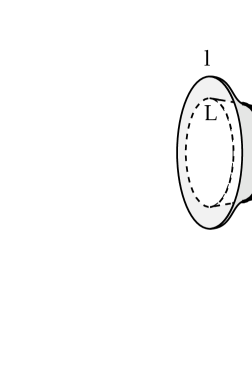
FIG. 2.: (a) A portion of a surface with area $A$ and boundary length $L$, (b) A disk with boundary length $l$ and effective boundary length $L<l$ is stretched so that an average point is further from the boundary

Another interesting feature of the bulk magnetization is that when expressed in terms of the rescaled boundary length $L$ it is independent of $h$, except where $h=0$, when the magnetization vanishes. This result indicates that just as in flat space, any nonzero magnetic field produces a renormalization group flow whose fixed point limit is the infinite magnetic field boundary condition.

Finally, it should be noted that of the results presented here, the scaling factor $\alpha(h)$ in (7) and the explicit form of the magnetization (12) have a functional dependence on $h$ which depends on the set of triangulations we have used for the disk. Just as in the case of the flat space Ising model, different choices of lattice discretization will give rise to different critical values $g_{c}$, different rescaling functions $\alpha(h)$, and boundary magnetizations with different functional dependence on $h$. Certain of the results obtained here – the functional dependences of the disk partition function and the bulk magnetization on the rescaled boundary length $L$ and area $A$, and the fact that the boundary magnetic susceptibility is finite and nonzero – should be independent of the choice of discretization, however, and should give the same continuum limit in any formulation of the theory. On the other hand, the result that the bulk magnetization decreases with increasing boundary field is not necessarily a universal result, since it depends upon the explicit form of the rescaling function $\alpha(h)$.

- [1]
- [2] Electronic address: carroll@marie.mit.edu
- [3] Electronic address: m.ortiz@ic.ac.uk
- [4] Electronic address: wati@princeton.edu
- [5] B. M. McCoy and T. T. Wu, Phys. Rev. 162, 436 (1967); Phys. Rev. 174, 546 (1968); The two-dimensional Ising model (Harvard University Press, 1973).
- [6] S. Ghoshal and A. Zamolodchikov, Int. J. Mod. Phys. A9 (1994) 3841, hep-th/9306002; Erratum: A9, 4353.
- [7] R. Chatterjee and A. Zamolodchikov, Mod. Phys. Lett. A9 (1994) 2227, hep-th/9311165.
- [8] R. Konik, A. LeClair and G. Mussardo On Ising correlation functions with boundary magnetic field, hep-th/9508099, August 1995.
- [9] J. Cardy, Nucl. Phys. B324 (1989) 581.
- [10] I. Affleck and A. Ludwig, Phys. Rev. Lett. 67, 161 (1991).
- [11] J. Polchinski Phys. Rev. Lett. 75, 4724 (1995), hep-th/9510017.
- [12] F. David, Mod. Phys. Lett. A3 (1988) 1651; J. Distler and H. Kawai, Nucl. Phys. B321 (1989) 509.
- [13] V. G. Knizhnik, A. M. Polyakov, and A. B. Zamolodchikov, Mod. Phys. Lett. A3 (1988) 819.
- [14] V. Kazakov, Phys. Lett. 119A (1987) 140; D. V. Boulatov and V. A. Kazakov, Phys. Lett. 186B (1987) 379.
- [15] S. M. Carroll, M. E. Ortiz and W. Taylor IV, to appear in Nuclear Physics B, hep-th/9510199.
- [16] S. M. Carroll, M. E. Ortiz and W. Taylor IV, to appear in Nuclear Physics B, hep-th/9510208.
- [17] M. Staudacher, Phys. Lett. B305 (1993) 332, hep-th/9301038.
- [18] M. R. Douglas and M. Li, Phys. Lett. B348 (1995) 360, hep-th/9412203.
- [19] G. Moore, N. Seiberg, and M. Staudacher, Nucl. Phys. B362 (1991) 665.
- [20] E. Gava and K. S. Narain, Phys. Lett. 263B (1991) 213.
- [21] I. Kostov, Mod. Phys. Lett. A4 (1989) 217.