hep-th/9605089

ZU-TH 13/96

May 1996

Cosmological Analogues of the

Bartnik–McKinnon Solutions

M.S. Volkov, N. Straumann, G. Lavrelashvili,

M. Heusler and O. Brodbeck

Institut für Theoretische Physik, Universität Zürich
Winterthurerstrasse 190, CH–8057 Zürich, Switzerland

Abstract

We present a numerical classification of the spherically symmetric, static solutions to the Einstein–Yang–Mills equations with cosmological constant $\Lambda$. We find three qualitatively different classes of configurations, where the solutions in each class are characterized by the value of $\Lambda$ and the number of nodes, $n$, of the Yang–Mills amplitude.

For sufficiently small, positive values of the cosmological constant, $\Lambda<\Lambda_{\mbox{\scriptsize crit}}(n)$, the solutions generalize the Bartnik–McKinnon solitons, which are now surrounded by a cosmological horizon and approach the deSitter geometry in the asymptotic region. For a discrete set of values $\Lambda_{\rm reg}(n)>\Lambda_{\rm crit}(n)$, the solutions are topologically $3$–spheres, the ground state $(n=1)$ being the Einstein Universe. In the intermediate region, that is for $\Lambda_{\mbox{\scriptsize crit}}(n)<\Lambda<\Lambda_{\mbox{\scriptsize reg}}(n)$, there exists a discrete family of global solutions with horizon and “finite size”.

1 Introduction

The interplay of gravity and non–linear field theoretical matter models leads to a wealth of new and surprising phenomena. In particular, there has been an increasing interest in both the structure and the stability of black hole solutions “with hair”. (See, e.g., [3] and [4] for some key references.) Moreover, self–gravitating field theories have also become very popular in cosmology in connection with various inflationary scenarios, the formation of topological defects in cosmological phase transitions, etc.

In this paper we present and discuss some new solutions with various global properties of the Einstein–Yang–Mills (EYM) system with cosmological constant $\Lambda$. For a limited range of the “bifurcation parameter” $\Lambda$ we find a class of solutions which can be viewed as a continuation of the remarkable discrete family of particle–like solutions discovered by Bartnik and McKinnon (BK) for $\Lambda=0$ [2]. In the vicinity of the origin, these solutions resemble the BK solitons. However, the solutions are surrounded by a cosmological horizon and approach deSitter spacetime in the asymptotic region. For each node number, $n$, these asymptotically deSitter solutions exist only for sufficiently small cosmological constants, $0<\Lambda\leq\Lambda_{\mbox{\scriptsize crit}}(n)$, where we determine $\Lambda_{\mbox{\scriptsize crit}}(n)$ numerically.

When $\Lambda$ exceeds $\Lambda_{\mbox{\scriptsize crit}}(n)$ we obtain a different class of solutions, for which the $2$–spheres (i.e., orbits belonging to the assumed SO$(3)$ symmetry) reach their maximal size outside the cosmological horizon. The position of the maximal sphere, $S^{2}_{\mbox{\scriptsize max}}$, moves inwards as $\Lambda$ increases and approaches the horizon when $\Lambda$ tends to some special value $\Lambda_{\star}(n)$, say. Outside $S^{2}_{\mbox{\scriptsize max}}$ a true singularity develops. This region resembles the interior of a black hole solution, whose singularity is also shielded by a horizon. For obvious reasons, we call these solutions bag of gold configurations.

These bag of gold solutions continue to exist for $\Lambda_{\mbox{\scriptsize crit}}(n)<\Lambda<\Lambda_{\star}(n)$, where the extremal sphere now lies inside the horizon. An interesting phenomenon occurs when $\Lambda$ reaches the upper limit $\Lambda_{\mbox{\scriptsize reg}}(n)$, for which the singularity approaches the horizon. For $\Lambda=\Lambda_{\mbox{\scriptsize reg}}(n)$ an everywhere regular, spatially compact solution exists for all $n$. In the special case where $n=1$ this is precisely the Einstein Universe with a constant energy density of the Yang–Mills field on $S^{3}$. This particular solution has repeatedly been rediscovered in the past [5]. For higher node numbers, the spatial part of the manifold is a “squashed” $3$–sphere, and the solutions can only be constructed numerically.

As is the case for the BK family, it would be valuable to have an existence proof for the compact solutions, probably along similar lines as presented in [6], [7]. We would also like to mention Ref. [8] on EYM solutions with cosmological constant, which contains some partial results of the present paper.

A crucial issue is the question of stability of the solutions presented in this paper. However, it turned out that this is a quite involved and subtle problem, mainly for topological reasons. We shall therefore present this part of our investigation in an accompanying paper [9].

This article is organized as follows: In the second and third sections we derive the basic equations and present some special solutions which can be given in closed form. The fourth and fifth sections are devoted to the asymptotically deSitter solutions and their analytic extensions, respectively. The bag of gold configurations are described in the sixth section. Finally, in the last section, we discuss the globally regular, compact solutions.

2 Basic Equations

We consider an EYM model with cosmological constant $\Lambda$ and action

$$S\,=\,-\frac{1}{4\pi}\int\left[\,\frac{1}{4G}\,\ast\,({\cal R}-2\Lambda)\,+\,\frac{1}{2g^{2}}\,\mbox{tr}\,(F\wedge\ast F)\,\right]\,,$$ (1)

where $G$ is Newton’s constant and $g$ denotes the gauge coupling constant. Since we restrict ourselves to configurations with spherical symmetry, the spacetime manifold $(M,\mbox{\boldmath$g$})$ has (locally) the structure of a warped product, $M=\tilde{M}\times_{R}S^{2}$, with metric

$$\mbox{\boldmath$g$}\,=\,\tilde{\mbox{\boldmath$g$}}\,+\,R^{2}\,\hat{\mbox{\boldmath$g$}}\,.$$ (2)

Here, $\tilde{\mbox{\boldmath$g$}}$ and $\hat{\mbox{\boldmath$g$}}$ denote the metrics on $\tilde{M}$ and $S^{2}$, respectively, and $R$ is a function on $\tilde{M}$. Throughout this paper, quantities referring to $(\tilde{M},\tilde{\mbox{\boldmath$g$}})$ are endowed with a tilde and those for $(S^{2},\hat{\mbox{\boldmath$g$}})$ with a hat. The Einstein tensor for warped product manifolds becomes [3]

$$G_{ab} = \frac{2}{R}\left[\tilde{g}_{ab}\tilde{\hbox{\hskip 1.42262pt\hbox{\vrule width=6.54413pt,height=0.56905pt\vbox{\hrule width=0.85358pt,height=7.39772pt}\hskip-7.39772pt\vbox{\hbox{\vrule width=7.39772pt,height=0.28453pt} \vskip-0.28453pt\hrule width=0.28453pt,height=7.39772pt}}\hskip 1.42262pt}}R-\tilde{\nabla}_{a}\tilde{\nabla}_{b}R\right]\,+\,\frac{1}{R^{2}}\tilde{g}_{ab}\left[(dR|dR)-1\right]\,,$$ (3)

$$G_{Ab} = 0\,,$$ (4)

$$G_{AB} = R^{2}\hat{g}_{AB}\left[\frac{1}{R}\tilde{\hbox{\hskip 1.42262pt\hbox{\vrule width=6.54413pt,height=0.56905pt\vbox{\hrule width=0.85358pt,height=7.39772pt}\hskip-7.39772pt\vbox{\hbox{\vrule width=7.39772pt,height=0.28453pt} \vskip-0.28453pt\hrule width=0.28453pt,height=7.39772pt}}\hskip 1.42262pt}}R-\frac{1}{2}\tilde{\cal R}\right]\,,$$ (5)

where $\tilde{\cal R}$ denotes the Ricci scalar of $(\tilde{M},\tilde{\mbox{\boldmath$g$}})$. (Small and capital Latin letters are used for indices on $(\tilde{M},\tilde{\mbox{\boldmath$g$}})$ and $(S^{2},\hat{\mbox{\boldmath$g$}})$, respectively; $a,\ b,\ c\ =0,\ 1$ and $A,\ B,\ C\ =2,\ 3$.) With respect to the diagonal parametrization of the metric $\tilde{\mbox{\boldmath$g$}}$,

$$\tilde{\mbox{\boldmath$g$}}\,=\,-\,e^{2a(t,\rho)}\,dt^{2}\,+\,e^{2b(t,\rho)}\,d\rho^{2}\,,$$ (6)

which we shall often use in this paper, the d’Alembertian of a function $R$, say, and the Ricci scalar on $(\tilde{M},\tilde{\mbox{\boldmath$g$}})$ are

$$\tilde{\hbox{\hskip 1.42262pt\hbox{\vrule width=6.54413pt,height=0.56905pt\vbox{\hrule width=0.85358pt,height=7.39772pt}\hskip-7.39772pt\vbox{\hbox{\vrule width=7.39772pt,height=0.28453pt} \vskip-0.28453pt\hrule width=0.28453pt,height=7.39772pt}}\hskip 1.42262pt}}R\,=\,e^{-(a+b)}\left[\,(e^{a-b}R^{\prime})^{\prime}-(e^{b-a}\dot{R})\,\dot{}\,\right]$$ (7)

and

$$\tilde{\cal R}\,=\,-2\,e^{-(a+b)}\left[\,(e^{a-b}a^{\prime})^{\prime}-(e^{b-a}\dot{b})\,\dot{}\,\right]\,,$$ (8)

respectively.

For $SU(2)$, the spherically symmetric gauge potential has the general form

$$A\,=\,a\,\hat{\tau}_{\rho}\,+\,\varpi\,[\hat{\tau}_{\vartheta}d\vartheta+\hat{\tau}_{\varphi}\sin\vartheta d\varphi]\,+\,(w-1)\,[\hat{\tau}_{\varphi}d\vartheta-\hat{\tau}_{\vartheta}\sin\vartheta d\varphi]\,,$$ (9)

where $a=a_{0}dt+a_{1}d\rho$, and $a_{0}$, $a_{1}$, $w$ and $\varpi$ are functions on $\tilde{M}$. Here $\hat{\tau}_{\rho}=n^{i}\tau^{i}/2$, $\hat{\tau}_{\vartheta}=\partial_{\vartheta}\hat{\tau}_{\rho}$, $\hat{\tau}_{\varphi}=\partial_{\varphi}\hat{\tau}_{\rho}/\sin\vartheta$ and $n^{i}=(\sin\vartheta\cos\varphi,\sin\vartheta\sin\varphi,\cos\vartheta)$, where $\tau^{i}$ are the Pauli matrices. In the static, purely magnetic case the choice $a=\varpi=0$ is compatible with the field equations. The gauge potential (9) now reduces to

$$A\,=\,(w-1)\,[\,\hat{\tau}_{\varphi}\,d\vartheta\,-\,\hat{\tau}_{\vartheta}\sin\vartheta\,d\varphi\,]\,.$$ (10)

In terms of $w$, the stress–energy tensor has the components

$$8\pi g^{2}T_{ab} = \frac{1}{R^{2}}\left[w,_{a}w,_{b}\,-\,\tilde{g}_{ab}\,\left(\frac{1}{2}(dw|dw)+\frac{V(w)}{4\,R^{2}}\right)\right],$$ (11)

$$8\pi g^{2}T_{Ab} = 0\,,$$ (12)

$$8\pi g^{2}T_{AB} = \hat{g}_{AB}\,\frac{V(w)}{4\,R^{2}}\,,$$ (13)

with $V(w)=(1-w^{2})^{2}$.

With respect to the parametrization (6) of the metric $\tilde{\mbox{\boldmath$g$}}$, the static field equations assume the form

$$-\,e^{-2b}\,\left[\mu^{\prime\prime}+\mu^{\prime}\,(\mu^{\prime}-a^{\prime}-b^{\prime})\right] = \kappa\;e^{-2b}\,\frac{w^{\prime 2}}{R^{2}}\,,$$ (14)

$$\frac{1}{R^{2}}\,-\,e^{-2b}\,\left[\mu^{\prime\prime}+\mu^{\prime}\,(2\mu^{\prime}+a^{\prime}-b^{\prime})\right] = \kappa\;\frac{V(w)}{2\,R^{4}}\,+\,\Lambda\,,$$ (15)

$$\;\;\frac{1}{R^{2}}\,+\,e^{-2b}\,\left[a^{\prime\prime}+a^{\prime}\,(a^{\prime}-b^{\prime})-\mu^{\prime 2}\right] = \kappa\;\frac{V(w)}{R^{4}}\,,$$ (16)

and

$$e^{-(a+b)}\,(e^{a-b}\,w^{\prime})^{\prime}\,=\,\frac{1}{4\,R^{2}}\,V,_{w}\,,$$ (17)

where we have introduced $e^{\mu}\equiv R$ and where eqs. (14), (15) and (16) are the $\frac{1}{2}(00+11)$, $\frac{1}{2}(00-11)$ and $\frac{1}{2}(00+11-22-33)$ components of the Einstein equations. We also note that the (dimension–full) coupling constant $\kappa=8\pi G/g^{2}$ can be absorbed by introducing the dimensionless quantities $R/\sqrt{\kappa}$, $\rho/\sqrt{\kappa}$ and $\Lambda\kappa$. (We shall often set $\kappa=2$ in this paper, that is, we measure length, time and mass in units of $[Gg^{2}c^{-4}]$, $[G^{1/2}gc^{-3}]$ and $[g^{2}G^{-1}]$, respectively; see [10].)

We shall use two gauges in this paper, depending on whether or not $R$ has a local maximum. Considering solutions for which $R$ has no critical point, we can use Schwarzschild coordinates, that is, we are alowed to choose the gauge

$$R(\rho)\,=\,\rho\,\equiv\,r\,.$$ (18)

It is then also convenient to introduce the functions $N(r)$ and $\sigma(r)$, defined by

$$N\,\equiv\,(dr|dr)\,=\,e^{-2b}\,,\;\;\;\;\;\sigma\,\equiv\,\sqrt{-\tilde{g}}\,=\,e^{a+b}\,.$$ (19)

In terms of this parametrization, the static equations (14), (15) and (17) become

$$\sigma^{\prime}\,=\,\kappa\,\frac{w^{\prime 2}}{r}\,\sigma\,,$$ (20)

$$m^{\prime}\,=\,\frac{\kappa}{2}\,\left[N\,w^{\prime 2}\,+\,\frac{V(w)}{2\,r^{2}}\right]\,,$$ (21)

$$N\,w^{\prime\prime}\,+\,\frac{w^{\prime}}{r}\,\left[\frac{2m}{r}-\frac{2}{3}\Lambda r^{2}-\kappa\frac{V}{2r^{2}}\right]\,=\,\frac{V,_{w}}{4\,r^{2}}\,,$$ (22)

where a dash denotes the derivative with respect to $r$. Here we have already used eq. (20) in the second and the third equations, in order to eliminate the metric function $\sigma$. The function $m(r)$ is defined by the relation

$$N(r)\,\equiv\,1\,-\,\frac{2m(r)}{r}\,-\,\frac{\Lambda}{3}\,r^{2}\,.$$ (23)

When considering solutions for which $R$ develops a local extremum, we use the gauge $a+b=0$, that is, we parametrize the static metric by the two functions $R(\rho)$ and $Q(\rho)$, where

$$Q(\rho)\,\equiv\,e^{2a}\,=\,e^{-2b}\,.$$ (24)

The static field equations (14), (16) and (17) then assume the form

$$R^{\prime\prime}\,=\,-\,\kappa\;\frac{w^{\prime 2}}{R}\,,$$ (25)

$$Q^{\prime\prime}\,=\,2Q(\frac{R^{\prime}}{R})^{2}\,-\frac{2}{R^{2}}\,+\,\kappa\,\frac{2V(w)}{R^{4}}\,,$$ (26)

$$\left(Q\,w^{\prime}\right)^{\prime}\,=\,\frac{V,_{w}}{4\,R^{2}}\,,$$ (27)

where now $Q^{\prime}\equiv dQ/d\rho$, etc. Using eq. (25), the remaining equation (15) becomes a first integral,

$$(Q\,R)^{\prime}\,R^{\prime}\,=\,\kappa\,\left(Qw^{\prime 2}\,-\,\frac{V(w)}{2\,R^{2}}\right)\,+\,1\,-\,\Lambda R^{2}\,.$$ (28)

It is clear that this coordinate system is also suited to discuss solutions for which $R$ has no critical points. However, for obvious reasons, we prefer to use the familiar parametrization (18), (19) in those cases.

3 Special Solutions

Before we present a classification of the static configurations, we consider some special solutions which can be given in closed form.

First, for $R(\rho)=\rho$ and constant Yang–Mills amplitude, we find from eqs. (25)-(28) above:

$$R(\rho)\,=\,\rho,\ \ \ \ w(\rho)\,=\,0,\pm 1,\ \ \ \ Q(\rho)\,=\,1\,-\,\frac{2M}{\rho}\,+\,\kappa\,\frac{V(w)}{2\rho^{2}}\,-\,\frac{\Lambda}{3}\rho^{2},$$ (29)

with $M$ being a constant of integration. For $w=0$ ($V=1$) this solution corresponds to the Reissner–Nordström–deSitter Universe with unit magnetic charge, whereas we obtain the Schwarzschild–deSitter solution for $w=\pm 1$ ($V=0$).

Next, we consider solutions for which both $R(\rho)$ and $w(\rho)$ are constants. For $V(w)=0$ one easily finds

$$R(\rho)\,=\,\frac{1}{\sqrt{\Lambda}},\ \ \ \ w(\rho)\,=\,\pm 1,\ \ \ \ Q(\rho)\,=\,-\,\Lambda\rho^{2}\,+\,A\rho\,+\,B\,,$$ (30)

which corresponds to the $H^{2}\times S^{2}$ Nariai solution [11]. (Here $A$ and $B$ are constants of integration.) If $w=0$, we find for sufficiently small values of the cosmological constant, $\Lambda\leq(2\kappa)^{-1}$,

$$R^{2}(\rho)\,=\,\frac{1\pm\sqrt{1-2\kappa\Lambda}}{2\Lambda}\,,\ \ \ w(\rho)\,=\,0,\ \ \ \ Q(\rho)\,=\,\frac{1}{R^{2}}(\frac{\kappa}{R^{2}}-1)\rho^{2}\,+\,A\rho\,+\,B\,.$$ (31)

In the limit of vanishing $\Lambda$ the solution with the lower sign reduces to the magnetic Robinson–Bertotti Universe (with $R^{2}=\frac{1}{2}\kappa$).

Finally, there exists a solution for which the components of the stress–energy tensor assume constant values without $w(\rho)$ being a constant. This is possible only for the special value $\Lambda=3/(2\kappa)$. In fact,

$$R(\rho)\,=\,\sqrt{\kappa}\,\sin({\rho\over\sqrt{\kappa}}),\ \ \ w(\rho)\,=\,\cos({\rho\over\sqrt{\kappa}}),\ \ \ Q(\rho)\,=\,1$$ (32)

describes the static Einstein Universe.

The above examples indicate that the qualitative behavior of the static solutions to eqs. (14)-(17) crucially depends on the value of the cosmological constant. In the following, we shall present a classification of these solutions in terms of $\Lambda$ and the node number of $w$.

4 Asymptotically deSitter Solutions

We start our numerical investigation by considering small values of $\Lambda$. For $\Lambda=0$ the regular, asymptotically flat solutions of the EYM equations were found by Bartnik and McKinnon in 1988 [2] and, since then, have been subject to numerous studies (see, e.g. [3], [4], [7] and references therein). Each solution has a typical size, $R_{n}$, where $n$ is the number of nodes of the YM amplitude $w$. In the region $R>R_{n}$ the energy density of the Yang–Mills field decays rapidly, and the metric approaches the vacuum Schwarzschild metric.

For small values of the cosmological constant, $\Lambda\ll 1/R^{2}_{n}$, the contribution $\Lambda R^{2}$ to the energy density is negligible. For $R<R_{n}$, one therefore expects that the solutions do not considerably deviate from the BK solutions. In the region $r>R_{n}$, however, the effect of $\Lambda$ becomes significant, which suggests that the metric approaches the deSitter metric. Hence – for sufficiently small values of the cosmological constant – the solutions are expected to resemble the regular BK solitons, which are surrounded by a cosmological horizon at $R\sim 1/\sqrt{\Lambda}$ and approach the deSitter geometry in the asymptotic region.

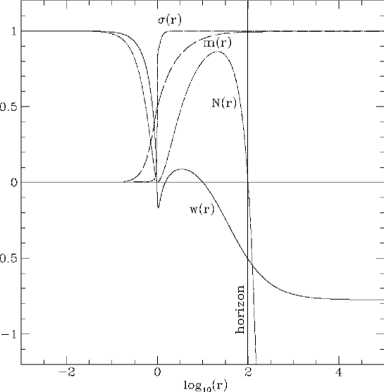
Figure 1: Asymptotically deSitter solution with $\Lambda=3\times 10^{-4}$ and $n=3$. For this solution one finds $b=0.6998$, $r_{h}=98.99$, $w_{h}=-0.505$, $w_{\infty}=-0.774$, $M=m(\infty)=0.994$, $a=-37$, $\sigma(0)=2\times 10^{-3}$, $\sigma(r_{h})=0.99999$ and $N_{min}=1.7\times 10^{-3}$.

The numerical analysis of eqs. (20)-(22) confirms these expectations. In order to find numerical solutions, we need the formal power series expansions of the equations (21) and (22) in the vicinity of the origin, $r=0$, the cosmological horizon, $r=r_{h}$, and for $r\rightarrow\infty$. In the vicinity of the origin, the regular solutions behave as follows ($\kappa=2$):

$$w\,=\,1-br^{2}+{\cal O}(r^{4}),\ \ \ \ \ \ N\,=\,1-(4b^{2}+{\Lambda\over 3})r^{2}+{\cal O}(r^{4})\,.$$ (33)

Near the horizon, defined by $N(r_{h})=0$, we find with $x=r-r_{h}$:

$$w\,=w_{h}+w^{\prime}_{h}\,x+{\cal O}(x^{2}),\ \ \ \ \ \ N\,=\,N^{\prime}_{h}\,x+{\cal O}(x^{2})\,,$$ (34)

where

$$N^{\prime}_{h}\,=\,\frac{1}{r_{h}}(1-\frac{V(w_{h})}{r_{h}^{2}}-\Lambda r_{h}^{2})\ <0\ \ \ {\rm and}\ \ \ w^{\prime}_{h}\,=\,\frac{V,_{w}(w_{h})}{4r^{2}_{h}N^{\prime}_{h}}\,.$$ (35)

Finally, in the asymptotic regime, $r\rightarrow\infty$, we have

$$w\,=\,w_{\infty}\,+\,\frac{a}{r}\,-\,\frac{3V,_{w}(w_{\infty})}{8\,\Lambda}\frac{1}{r^{2}}\,+\,{\cal O}(\frac{1}{r^{3}})\,,$$

$$N\,=\,1\,-\,\frac{2M}{r}\,-\,\frac{\Lambda}{3}\,r^{2}\,+\,[V(w_{\infty})-\frac{2}{3}\Lambda a^{2}]\frac{1}{r^{2}}\,+\,{\cal O}(\frac{1}{r^{3}})\,.$$ (36)

Here, $b$, $r_{h}$, $W_{h}$, $W_{\infty}$, $M$ and $a$ are six “shooting” parameters.

In order to obtain numerical solutions to the static equations one starts the integration with the expansions (33) and (34) and tries to match the functions $w$, $w^{\prime}$ and $N$ at some intermediate point between the origin and the horizon. The three matching conditions then fix the values of the parameters $b$, $r_{h}$ and $w_{h}$ appearing in eqs. (33) and (34). Subsequently, one uses the remaining three parameters in eq. (36) to match the solutions obtained from numerically integrating between the horizon and infinity. Finally, the remaining metric function $\sigma$ is obtained from eq. (20), where $\sigma$ behaves like

$$\sigma\,=\,\sigma(0)+{\cal O}(r^{2}),\ \ \ \sigma\,=\,\sigma(r_{h})+{\cal O}(r-r_{h}),\ \ \ \sigma\,=\,1+{\cal O}(\frac{1}{r^{4}}),\ \ \$$ (37)

in the vicinity of the origin, the horizon and infinity, respectively (see Fig.1).

The numerical procedure yields the following result: For each fixed value of $\Lambda\ll 1$ we recover a family of solutions which correspond to the $\Lambda=0$ BK solitons. Each solution is characterized by the value of $\Lambda$ and the number, $n$, of nodes of $w$ inside the cosmological horizon. Outside the horizon $w$ tends to a constant value, $w_{\infty}$, say. Since $w_{\infty}\neq\pm 1$, the YM field gives rise to the magnetic charge ${\cal P}=[2\,\mbox{tr}(P\cdot P)]^{1/2}=w^{2}_{\infty}-1$, where

$$P\,=\,\frac{1}{4\pi}\oint_{S^{2}}\,F\,,$$ (38)

and where the integration is performed over the $2$–sphere at spatial infinity. Here we have used eq. (10) and $F=dA+A\wedge A$ to obtain $F=(w^{2}-1)\hat{\tau}_{\rho}d\Omega+(w-1)^{-1}dw\wedge A$. (It is worthwhile recalling that the solutions with $\Lambda=0$ have vanishing magnetic charge.) The metric asymptotically approaches the Reissner–Nordström–deSitter metric with effective charge $[P^{2}-2\Lambda a^{2}/3]^{1/2}$; see eq.(36).

5 Analytic Extensions

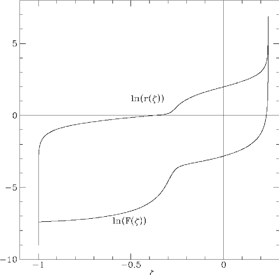
Figure 2: The functions $r(\zeta)$ and $F(\zeta)$ for the asymptotically deSitter solution with $\Lambda=3\times 10^{-4}$, $n=2$. For this solution one has $F(0)=6\times 10^{-4}$ and $\zeta_{\infty}=0.24$.

In this section we construct the analytic extension for a generic metric of the above type. Our first goal is to write the metric $\tilde{\mbox{\boldmath$g$}}$ in conformally flat form, such that the spacetime metric becomes

$$\mbox{\boldmath$g$}\,=\,\sigma^{2}\,N\,(dt^{2}-d\chi^{2})\,-\,r^{2}d\Omega^{2}\,.$$ (39)

In order to do so, we need the following essential properties of the solutions discussed above: Both $N$ and $\sigma$ are smooth functions, where $\sigma(r)$ is bounded and everywhere positive. The metric function $N(r)$ is subject to the boundary conditions $N(0)=1$ and $N\rightarrow-c^{2}r^{2}$ as $r\rightarrow\infty$. Moreover, $N(r)$ changes sign exactly once, namely at the horizon, $N(r_{h})=0$. By virtue of these properties, the new radial coordinate $\chi$,

$$\chi(r)=\int_{0}^{r}\frac{d\bar{r}}{\sigma N}\,,\ \ r<r_{h},\ \ \ {\rm and}\ \ \ \chi(r)=\chi_{\infty}-\int_{r}^{\infty}\frac{d\bar{r}}{\sigma N},\ \ r>r_{h}$$ (40)

increases from zero to infinity as $r$ runs from zero to $r_{h}$, and then decreases from infinity to $\chi_{\infty}$ as $r$ grows from $r_{h}$ to infinity. The constant $\chi_{\infty}$ is fixed by considering the expansion of the above integrals in the vicinity of the horizon,

$$\chi=-\frac{1}{2\eta}\ln|r-r_{h}|+C+{\cal O}(r-r_{h})\,,\ \ \ |r-r_{h}|\ll 1\,,$$ (41)

and requiring that the constant $C$ has the same value in both cases. Here we have also introduced the quantity $\eta$,

$$\eta\,=\,-\,\frac{1}{2}\,\sigma\,N^{\prime}\left|{}_{r=r_{h}}\,>\,0\,,\right.$$ (42)

which does not vanish for a regular horizon. With respect to $\chi$, the metric now assumes the desired form (39) which, in a neighborhood of the horizon, becomes

$$\mbox{\boldmath$g$}\,=\,\pm\sigma(r_{h})\,\eta\,e^{-2\eta\chi}\,[1+{\cal O}(e^{-2\eta\chi})]\,(dt^{2}-d\chi^{2})\,-\,r^{2}d\Omega^{2}\,,$$ (43)

where the plus and minus signs refer to the regions $r<r_{h}$ and $r>r_{h}$, respectively.

Figure 3: Spacetime diagram for the asymptotically deSitter solution with $\Lambda=3\times 10^{-4}$, $n=2$.

Next, we note that $\zeta(r)$, defined by

$$\zeta(r)\,=\,-e^{-2\eta\chi(r)},\ \ \ r<r_{h}\,,\ \ \ \ \ \ \ \ {\rm and}\ \ \ \ \zeta(r)\,=\,e^{-2\eta\chi(r)},\ \ \ r>r_{h}\,,$$ (44)

is a monotonically increasing function of $r$ with $\zeta(0)=-1$, $\zeta(r_{h})=0$ and $\zeta\rightarrow\exp(-2\eta\chi_{\infty})>0$ as $r\rightarrow\infty$. Hence, the inverse function, $r(\zeta)$, is well–defined and the function $F(\zeta)$,

$$F(\zeta)\,=\,-\,\frac{\eta^{2}}{\zeta}\,\sigma^{2}(r(\zeta))\,N(r(\zeta))\,,$$ (45)

is therefore smooth and everywhere positive. As usual, one finally passes from the coordinates $(t,\chi)$ to the new coordinates $(U,V)$, where

$$U = e^{-\eta\chi}\sinh\eta\chi,\ \ \ \ \ V=e^{-\eta\chi}\cosh\eta\chi,\ \ \ \ r<r_{h}\,,$$

$$U = e^{-\eta\chi}\cosh\eta\chi,\ \ \ \ \ V=e^{-\eta\chi}\sinh\eta\chi,\ \ \ \ r>r_{h}\,.$$ (46)

The analytically extended metric eventually becomes

$$\mbox{\boldmath$g$}\,=\,F(\zeta)\,(dU^{2}-dV^{2})\,-\,r^{2}(\zeta)\,d\Omega^{2},$$ (47)

where $\zeta=\zeta(U,V)=U^{2}-V^{2}$. The two functions $F(\zeta)$ and $r(\zeta)$ can be determined numerically (see Fig.2). For the deSitter solution one easily finds

$$F(\zeta)\,=\,\frac{4}{(1-\zeta)^{2}},\ \ \ \ r(\zeta)\,=\,\frac{1+\zeta}{1-\zeta},\ \ \ \ \zeta\in[-1,1].$$ (48)

The spacetime diagram in coordinates $(U,V)$ is displayed in Fig.3. The spacetime manifold corresponds to the region $U^{2}-V^{2}\in[-1,\zeta_{\infty}]$. The qualitative features of the diagram are identical with those of the deSitter solution.

Figure 4: The horizon radius $R_{h}$ versus the cosmological constant $\Lambda$ for the $n=1$ EYM solutions.

6 Bag of Gold Solutions

The asymptotically deSitter solutions described above exist only for sufficiently small values of the cosmological constant: For each fixed value of the node parameter $n$, there exists a maximal value $\Lambda_{\mbox{\scriptsize crit}}(n)$, say, beyond which the numerical analysis breaks down.

Solutions which belong to larger values of $\Lambda$ exhibit a local extremum of $R$ and cannot be obtained in Schwarzschild coordinates. We therefore pass to a parametrization of the metric for which $R(\rho)$ is a dynamical function and choose the gauge $e^{2a}=e^{-2b}\equiv Q(\rho)$; see eq. (24).

Equations (25)-(28) yield the formal power series at the origin ($\kappa=2$),

$$w\,=\,1-b\,\rho^{2}+{\cal O}(\rho^{4}),\ \ \ \ R\,=\,\rho+{\cal O}(\rho^{5}),\ \ \ \ Q\,=\,1+(4b^{2}-\frac{\Lambda}{3})\rho^{2}+{\cal O}(\rho^{4}),$$ (49)

where $b$ is the only free parameter. The numerical integration shows that $Q(\rho)$ develops a zero at some $\rho=\rho_{h}(b,\Lambda)$, indicating the presence of a horizon. Requiring that all curvature invariants remain finite at the horizon yields

$$\lim_{\rho\rightarrow\rho_{h}}\sqrt{Q}\,w^{\prime}\,=\,0\,.$$ (50)

Figure 5: Change of the topology of the EYM solutions. The solution with $\Lambda=\Lambda_{1}=0.3304$ is asymptotically deSitter, whereas the one with $\Lambda=\Lambda_{3}=0.3306$ is of the bag of gold type. The value $\Lambda=\Lambda_{2}=0.3305$ is very close to $\Lambda_{{\rm crit}}$. The functions $Q(\rho)$ and $w(\rho)$ for the three solutions are almost identical.

As a consequence of this condition we obtain a family of solutions between the origin and the horizon, which are parametrized by a discrete set of values $b_{n}(\Lambda)$, where $n$ is the number of nodes. The parameters $w_{h}$, $R_{h}$ and $R^{\prime}_{h}$ entering the power series at the horizon,

$$w=w_{h}+w^{\prime}_{h}x+{\cal O}(x^{2}),\ \ \ \ Q=Q^{\prime}_{h}x+{\cal O}(x^{2}),\ \ \ \ R=R_{h}+R^{\prime}_{h}x+O(x^{2}),\ \ \ \$$ (51)

are therefore fixed, once $b_{n}(\Lambda)$ is known. Here, $x=\rho-\rho_{h}$, and $Q^{\prime}_{h}$ and $w^{\prime}_{h}$ are given in terms of $w_{h}$, $R_{h}$ and $R^{\prime}_{h}$:

$$Q^{\prime}_{h}\,=\,\frac{1}{R_{h}\,R^{\prime}_{h}}\left(1-\frac{V(w_{h})}{R_{h}^{2}}-\Lambda R_{h}^{2}\right)\,,\ \ \ \ w^{\prime}_{h}\,=\,\frac{V,_{w}(w_{h})}{4R_{h}^{2}\,Q^{\prime}_{h}}\,.$$ (52)

Finally, we use this expansions to extend the solution beyond the horizon. The advantage of this procedure is that it essentially uses only one shooting parameter, $b$; the remaining parameters are then iteratively determined.

The numerical analysis reveals the following picture: For each value of the node number, the horizon radius $R_{h}$ decreases monotonically with increasing values of $\Lambda$, where $R_{h}\rightarrow\infty$ for $\Lambda\rightarrow 0$ and $R_{h}\rightarrow 0$ for $\Lambda\rightarrow\Lambda_{\mbox{\scriptsize reg}}(n)$ (see Fig.4). The limiting value $\Lambda_{\mbox{\scriptsize reg}}(n)$, for which the horizon shrinks to zero, decreases with growing node number $n$, where $\Lambda_{\mbox{\scriptsize reg}}(1)=3/4$ and $\Lambda_{\mbox{\scriptsize reg}}(\infty)=1/4$.

Figure 6: The bag of gold solution with $\Lambda=0.4$ and $n=1$.

Depending on the position of the maximum of $R$, one finds three qualitatively different classes of solutions, corresponding to the following subdivision of the interval $(0,\Lambda_{\mbox{\scriptsize reg}}(n))$ (see Fig.4).
(A) $0<\Lambda<\Lambda_{\mbox{\scriptsize crit}}(n)$: These are the deSitter like solutions discussed earlier. The function $R(\rho)$ has no critical points for finite values of $\rho$. In the asymptotic regime, $R^{\prime}(\rho)$ behaves like

$$R^{\prime}(\rho)=R^{\prime}_{\infty}+{\cal O}(\frac{1}{\rho})\ \ \ \ \ \ {\rm as}\ \ \ \rho\rightarrow\infty\,,$$ (53)

where the constant $R^{\prime}_{\infty}$ decreases with growing values of $\Lambda$ and vanishes for $\Lambda_{\mbox{\scriptsize crit}}(n)$. Thus, for $\Lambda\rightarrow\Lambda_{{\rm crit}}(n)$, $R(\rho)$ develops an “extremum at infinity”. The numerical analysis (see Fig.5) suggests that for $\Lambda=\Lambda_{{\rm crit}}(n)$, $R(\rho)$ asymptotically approaches a constant value, $R(\infty)=1/\sqrt{\Lambda_{{\rm crit}}(n)}$, whereas $w(\rho)$ tends to $\pm 1$; such that for $\rho\rightarrow\infty$ the solutions coincide with the Nariai solution (30). The topology of the solutions therefore changes for $\Lambda=\Lambda_{{\rm crit}}(n)$ (for the solution with one node one has $\Lambda_{\mbox{\scriptsize crit}}(1)=0.3305$).
(B) $\Lambda_{\mbox{\scriptsize crit}}(n)<\Lambda<\Lambda_{\star}(n)$: For these values of $\Lambda$ the function $R(\rho)$ develops a maximum for a finite value $\rho_{e}$ outside the horizon, $\rho_{h}<\rho_{e}<\infty$. Since $R^{\prime\prime}\leq 0$ (see eq. (25)), $R(\rho)$ decreases for $\rho>\rho_{e}$ and becomes zero at some finite value $\rho_{sing}$, say. In fact, the metric function $Q$ diverges as $\rho\rightarrow\rho_{sing}$, indicating that the geometry becomes singular. (For the solution with one node one finds $\Lambda_{\star}(1)=0.334$.)
(C) $\Lambda_{\star}(n)<\Lambda<\Lambda_{\mbox{\scriptsize reg}}(n)$: The behavior is similar to case (B). However, now $R$ reaches the maximal value inside the horizon, $\rho_{e}<\rho_{h}$. Since $\Lambda_{{\rm reg}}(n)$ is the maximal value for which the solutions exhibit a horizon, $R$ vanishes still outside the horizon, that is, $\rho_{sing}\geq\rho_{h}$. Again, $Q$ is unbounded for $\rho=\rho_{sing}$ (see Fig.6).

We call the solutions which exhibit a horizon and for which $R$ develops a second zero outside the horizon bag of gold solutions.

7 Compact Regular Solutions

Until now we have restricted our attention to solutions which develop a horizon. A new and interesting type of solutions is obtained in the limit $\Lambda\rightarrow\Lambda_{\mbox{\scriptsize reg}}(n)$, where the horizon and the singularity merge, $\rho_{h}\rightarrow\rho_{sing}$. In this limit, that is for $\Lambda=\Lambda_{\mbox{\scriptsize reg}}(n)$, the geometry turns out to be everywhere regular, in particular at both zeros of $R$. Moreover, the points where $R$ assumes its maximal value, $\rho_{e}$, lies precisely between these zeros and the spatial geometry is symmetric with respect to $\rho_{e}$. Since, in this case, the manifold has the topology of $I\!\!R\times S^{3}$, the zeros of $R$ and the $2$–sphere $\rho=\rho_{e}$ will be called the north pole, the south pole and the equator, respectively.

For each node number $n$, there exists precisely one value of the cosmological constant, $\Lambda=\Lambda_{\mbox{\scriptsize reg}}(n)$, for which one obtains compact solutions of the above kind. For $n=1$, the solution is the static Einstein Universe with $\Lambda_{\rm reg}(1)=3/(2\kappa)$, already presented in the second section:

$$R(\rho)\,=\,\sqrt{\kappa}\,\sin({\rho\over\sqrt{\kappa}}),\ \ \ w(\rho)\,=\,\cos({\rho\over\sqrt{\kappa}}),\ \ \ Q(\rho)\,=\,1\,.$$ (54)

The regular solutions with higher node numbers are obtained in the limit $\Lambda\rightarrow\Lambda_{\mbox{\scriptsize reg}}(n)$ from the corresponding bag of gold solutions. An alternative method, which takes advantage of the reflection symmetry with respect to the equator, is to integrate the field equations on the “northern hemisphere”, say. In order to do so, one has to impose boundary conditions at the pole (i.e., the origin, $\rho=0$) and the equator ($\rho=\rho_{e})$. The solutions are then obtained by matching the numerical integrations from the pole and the equator.

Figure 7: The $n=3$ compact solution.

The formal power series at the origin involve one “shooting” parameter, $b$, and were given in eq. (49). In order to obtain the series expansions in the vicinity of the equator, we have to distinguish two cases: Depending on whether the gauge field amplitude $w(\rho)$ is antisymmetric or symmetric with respect to $\rho_{e}$, the regular compact solutions will be called odd ($w_{e}=0$) or even ($w^{\prime}_{e}=0$), respectively.
(i) $w_{e}=0$: For the odd configurations one finds with $x=\rho-\rho_{e}$ ($\kappa=2$)

$$R\,=\,R_{e}+\frac{1}{2}R^{\prime\prime}_{e}\,x^{2}+{\cal O}(x^{4})\,,\;\;\;\;\;Q\,=\,Q_{e}+\frac{1}{2}Q^{\prime\prime}_{e}\,x^{2}+{\cal O}(x^{4})\,,$$

$$w\,=\,w^{\prime}_{e}\,x\,+\,{\cal O}(x^{3}),$$ (55)

where the field equations (25)-(28) imply that $w^{\prime}_{e}$, $R^{\prime\prime}_{e}$ and $Q^{\prime\prime}_{e}$ are given in terms of $R_{e}$ and $Q_{e}$,

$$w^{\prime 2}_{e}\,=\,\frac{1}{2Q_{e}}(R_{e}^{-2}+\Lambda R^{2}-1),\,\,\,\,\,\,R^{\prime\prime}_{e}\,=\,-\frac{2}{R_{e}}w^{\prime 2}_{e},\,\,\,\,\,\,Q^{\prime\prime}_{e}\,=\,\frac{2}{R_{e}^{4}}(2-R_{e}^{2})\,.$$

(ii) $w^{\prime}_{e}=0$: For solutions with even Yang–Mills amplitude we have

$$R\,=\,R_{e}+\frac{1}{4!}R^{(4)}_{e}\,x^{4}+{\cal O}(x^{6})\,,\;\;\;\;\;Q\,=\,Q_{e}+\frac{1}{2}Q^{\prime\prime}_{e}\,x^{2}+{\cal O}(x^{4})\,,$$

$$w\,=\,w_{e}\,+\,\frac{1}{2}w^{\prime\prime}_{e}\,x^{2}\,+\,{\cal O}(x^{4})\,.$$ (56)

As before, the only free parameters are $R_{e}$ and $Q_{e}$. In terms of these, $w_{e}$ is determined by eq. (28),

$$V(w_{e})\,=\,R_{e}^{2}\,\left(1-\Lambda\,R_{e}^{2}\right)\,,$$

and $w^{\prime\prime}_{e}$, $R^{(4)}_{e}$ and $Q^{\prime\prime}_{e}$ are obtained from eqs. (25)-(27),

$$(w^{\prime\prime}_{e})^{2}\,=\,\frac{Q_{e}}{4R^{2}_{e}}V,_{w}(w_{e}),\,\,\,\,\,\,R^{(4)}_{e}\,=\,-\frac{4}{R_{e}}(w^{\prime\prime}_{e})^{2},\,\,\,\,\,\,Q^{\prime\prime}_{e}\,=\,\frac{2}{R_{e}^{4}}(2V(w_{e})-R_{e}^{2})\,.$$

In both cases, the free parameters are the position of the horizon, $\rho_{e}$, the cosmological constant, the shooting parameter at the pole, $b$, and two independent shooting parameters at the equator (for instance $R_{e}$ and $Q_{e}$). The values of these quantities are presented in Table.1 for the first five compact solutions. The shape of the metric functions and the Yang–Mills amplitude is given in Fig.7 for the $n=3$ solution.

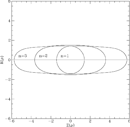
Figure 8: The embedding diagrams for the $n=1,2,3$ compact solutions.

Tab. 1. Parameters for compact solutions. $n$ $\Lambda$ $b$ $\sqrt{2}\rho_{e}/\pi$ $R_{e}/\sqrt{2}$ $w_{e}$ $Q_{e}$ 1 0.75 0.25 1 1 0 1 2 0.364244 0.429599 4.824 1.0150 $-0.5320$ 16.656 3 0.293218 0.508831 15.63 1.0757 0 88.390 4 0.270328 0.540489 39.64 1.0483 0.23549 417.12 5 0.260895 0.554021 88.43 1.0485 0 1409.7 … … … … … … … $\infty$ 0.25 0.569032 $\infty$ $1$ – $\infty$

The geometry of the compact solutions may be illustrated with the help of embedding diagrams. Consider the $3$-dimensional Euclidean space in cylindrical coordinates $R$, $Z$ and $\varphi$. A surface $S$ of revolution in this space is characterized by a mapping $\rho\rightarrow(R(\rho),Z(\rho))$, and the induced metric on $S$ is

$$\mbox{\boldmath$g$}_{S}\,=\,\left(R^{\prime 2}+Z^{\prime 2}\right)\,d\rho^{2}\,+\,R(\rho)^{2}\,d\varphi^{2}\,.$$ (57)

On the other hand, the metric of a spacelike section $S^{\prime}$ (with $t=t_{0}$ and $\vartheta=\pi/2$) through the geometry of the compact solutions is given by

$$\mbox{\boldmath$g$}_{S^{\prime}}\,=\,\frac{1}{Q(\rho)}\,d\rho^{2}\,+\,R(\rho)^{2}\,d\varphi^{2}\,.$$ (58)

Hence, the two geometries coincide, provided that we choose the function $Z(\rho)$ according to

$$Z(\rho)\,=\,Z(0)\,+\,\int_{0}^{\rho}\sqrt{1-Q(\bar{\rho})R^{\prime 2}(\bar{\rho})}\,\frac{d\bar{\rho}}{\sqrt{Q(\bar{\rho})}}\,,$$ (59)

where $\rho\in[0,2\rho_{e}]$.

The embedding diagrams $(R(\rho),Z(\rho))$ for the $n=1$, the $n=2$ and the $n=3$ compact regular solutions are presented in Fig.8. For $n=1$, we obtain the circle $(R(\rho),Z(\rho))=\sqrt{\kappa}(\sin(\rho/\sqrt{\kappa}),\cos(\rho/\sqrt{\kappa}))$, reflecting the fact that the manifold in this case is precisely $I\!\!R\times S^{3}$. The spatial sections of the solutions with higher values of $n$ resemble prolate ellipsoids (or “cigars”).

It is also instructive to draw the embedding diagrams for the solutions with horizon. In this case, the domain of integration in eq. (59) is $\rho\in[0,\rho_{h}]$, which yields half of the diagram. At the horizon one has $Q=0$ and therefore $dR/dZ=0$. Since $R(\rho_{h})\neq 0$, the horizon corresponds to the “throat” of the geometry, which connects the two identical patches of the manifold (see the conformal diagram in Fig.3). The resulting diagrams for several $n=1$ solutions are presented in Fig.9. The diagrams show that the throat becomes narrower as $\Lambda$ tends to the critical value $\Lambda_{\mbox{\scriptsize reg}}$, where the manifold splits into two separate pieces.

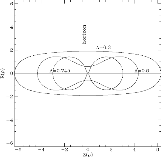
Figure 9: The embedding diagrams for the asymptotically deSitter solution with $\Lambda=0.3$, $n=1$, and for the $n=1$ bag of gold solutions with $\Lambda=0.6$ and $\Lambda=0.745$.

8 Concluding Remarks

The features of the static, spherically symmetric solutions to the EYM equations depend critically on the value of the cosmological constant $\Lambda$. For every node number $n$, there exists a globally regular, compact solution with $\Lambda=\Lambda_{\mbox{\scriptsize reg}}(n)$. For $\Lambda_{\mbox{\scriptsize crit}}(n)<\Lambda<\Lambda_{\mbox{\scriptsize reg}}(n)$, the configurations have “finite size” and exhibit a horizon. Finally, for sufficiently small values of the cosmological constant, $\Lambda<\Lambda_{\mbox{\scriptsize crit}}(n)$, the solutions generalize the BK solitons surrounded by a cosmological horizon.

In this paper, we have restricted our attention to solutions with a regular center. The extension to configurations with an event horizon is expected to be straightforward. In fact, we have no reasons to doubt that one will find a similar classification for these black hole solutions.

No globally regular solutions seem to exist for $\Lambda>\Lambda_{\mbox{\scriptsize reg}}(n)$. In this case, the metric function $Q(\rho)$ is everywhere positive and diverges as $\rho\rightarrow\rho_{sing}$, where $\rho_{sing}$ is the position of the second zero of $R(\rho)$. Such solutions may therefore be considered as bag of gold configurations without horizon. When $\Lambda$ is small and negative ($|\Lambda|\ll 1$), the solutions resemble again the BK solitons, however, they approach the anti–deSitter geometry in the asymptotic region.

We have also investigated the stability properties of the solutions presented in this paper. The stability analysis for these – asymptotically not flat – solutions is, however, rather involved. In particular, the fact that the size $R$ of the $2$–spheres develops a local maximum gives rise to the following difficulty: Either the pulsation equations assume the form of a regular, formally self-adjoint system with unphysical degrees of freedom, or one isolates the unphysical modes and obtains a singular pulsation equation. The methods by which these problems can be solved are presented in an accompanying paper [9], and here we merely mention the result: all of the solutions described above are unstable.

References

• [1]
• [2] R.Bartnik, J.McKinnon, Phys. Rev. Lett. 61, 141 (1988).
• [3] O.Brodbeck, M.Heusler, N.Straumann, Phys. Rev. D 53, 754 (1996).
• [4] N.E. Mavromatos, E.Winstanley, Phys. Rev. D 53, 3190 (1996).
• [5] J.Cervero, L.Jacobs, Phys. Lett. B 78, 427 (1978); M.Henneaux, J. Math. Phys. 23, 830 (1982); Y.Hosotani, Phys. Lett. B 147, 44 (1984).
• [6] J.A.Smoller, A.G.Wasserman, S.T.Yau, and J.B.McLeod, Commun. Math. Phys. 143, 115 (1991); J.A.Smoller, A.G.Wasserman, Commun. Math. Phys. 151, 303 (1993); ibid. 154, 377 (1993).
• [7] P.Breitenlohner, P.Forgacs, D.Maison, Commun. Math. Phys. 163, 141 (1994).
• [8] T.Torii, K.Maeda, T.Tachizawa, Phys. Rev. D 52, R4272 (1995).
• [9] O.Brodbeck, M.Heusler, G.Lavrelashvili, N.Straumann and M.S.Volkov, Stability Analysis of New Solutions of the EYM System with Cosmological Constant, ZU-TH 14/96.
• [10] G.Johnstone Stoney, Phil. Mag. (Ser 5) 11, 381 (1881).
• [11] H.Nariai, Science Reports of the Tohoku Univ. 35, 62 (1951).