4 D Quantum N-Dilaton Gravity
and
One-Loop Divergence of Effective Action
on Constant Dilaton

1 Introduction and Summary

Recently there has been considerable interest in the metric-scalar gravity in four dimensions from various point of view. Our point of view is that such a fundamental theory of quantum gravity is either a string theory or another theory like it. We will not resolve this issue. Furthermore, we do not remove the possibility that quantum gravity is a local field theory with renormalizability. A candidate for a consistent theory of quantized gravity is string theory. A low-energy effective theory of a string below the Plank scale represented by a metric and a dilaton is well known [1]. Such an effective action arises in the form of a power-series type of slope parameter ($\alpha^{\prime}$); the standard point of view is that the higher orders in such an expansion correspond to higher energies. From this point of view, at a lower energy scale the action for gravity has the form of a lower derivative dilaton action. Since the fundamental theory is not restricted to the string theory, we introduce N-dilations with the most general coupling to metric within two derivatives, such as (1.1). Although in the string theory there is no scalar field having such a coupling, we call our scalar fields dilatons by analogy. The Einstein gravity coupled to scalars is nonrenormalizable as naive power counting, and higher derivative gravity is renormalizable [2]; however, it is not unitary within a perturbation scheme [3]. Of course, it is not strange that a useful local field theory of gravity covering all energy regions does not exist. It is important to know whether a renormalizable local field theory of gravity constructed by metric exists or not, and what type of environment would allow its existence. Several studies, starting in seventies, have been performed to calculate the divergence of an effective action of four-dimensional gravity [4, 5, 6, 7, 9, 10]. In the pure Einstein action case without a cosmological term, it was originally calculated at the one-loop level by t’Hooft and Veltman [4]. They found that the action is not renormalizable off mass shell, but is finite on mass shell at the one-loop level. Furthermore, although the pure Einstein action with a cosmological constant is renormalizable [5], if one introduces matter fields the one loop renormalizability is lost, even on mass shell. Recently [7, 11] we considered the divergence of the effective action, which is the most general class with less than two derivatives for a scalar and a metric, while explicitly leaving the functions $A,B,\mathchar 28931\relax$ arbitrary. On an arbitrary back-ground space-time we found models which are finite in the case without a cosmological term, and with it are renormalizable by fine-tuning of functional form of $A(\phi),B(\phi),\mathchar 28931\relax(\phi)$ at the one loop level on mass shell. We have considered that on maximally symmetric background space-time the action (1.1) with $N=1$. Without any fine-tuning of the coupling functions $A(\phi)$, $B(\phi)$, we have shown that the divergence of the effective action has one term only which proportional to $\mathchar 28931\relax^{2}$, and the divergence can be renormalized easily. In the present paper we consider the action:

$$S\left[g_{\mu\nu},\phi_{i}\right]=\int d^{4}x\sqrt{-g}\;\left[A(\phi)_{ij}g^{\mu\nu}\partial_{\mu}\phi_{i}\partial_{\nu}\phi_{j}+B(\phi)R-2B(\phi)\mathchar 28931\relax(\phi)\right]\;\;\;i=1\cdots N$$ (1.1)

This is the most general class with less than two derivative for N scalars and a metric. Since by redefinition of fields $A_{ij}\longrightarrow A\delta_{ij}$ in generic, in this paper we consider $A_{ij}=A\delta_{ij}$ case only.

$$S\left[g_{\mu\nu},\phi_{i}\right]=\int d^{4}x\sqrt{-g}\;\left[A(\phi)g^{\mu\nu}\partial_{\mu}\phi_{i}\partial_{\nu}\phi_{i}+B(\phi)R-2B(\phi)\mathchar 28931\relax(\phi)\right]\;\;\;i=1\cdots N$$ (1.2)

Our paper is organized as follows. In section 2, we consider the classical analysis of the action (1.1). We show classically the non-equivalence between the class of action (1.1) and the class of the action without the kinetic term of the dilatons in (1.1). In section 3, we calculate the divergence of the effective action with the background field method and the Schwinger-Dewitt method. Especially, on constant dilaton background, we show an explicit calculation, and we get the structure of the divergence. In section 4, we restrict the form of the couplings in order to cancel a non-renormalizable term, and we show $N$ dependence of another non-renormalizable term which cannot be canceled in the case of $N\geq 1$. In section 5, we conclude this paper. We have three Appendixes.

2 Analysis at the Classical Level

We consider gravity with a general coupling to scalars in which the action is (1.1). In this section we analyze this theory at the classical level.

2.1. Classical Non-Equivalence between Constant and Non-Constant Dilaton Cases

In a previous paper[7] which treated the $N=1$ case in (1.1), we have shown the equivalence between an original action and the no kinetic term action. In this subsection, however, we show for $N>1$ a classical non-equivalence between the original action (1.2) and a model without kinetic term of dilaton ($\partial\phi_{i}=0$) in the original action (1.2). First we start with an action without kinetic terms of dilatons:

$$S\left[\bar{g}_{\mu\nu},\phi_{i}\right]=\int d^{4}x\sqrt{-\bar{g}}\;\left[{\cal B}(\phi)\bar{R}-2{\cal B}(\phi)\lambda(\phi)\right]\;\;\;$$ (2.1)

We transform the metric:

$$\bar{g_{\mu\nu}}\longrightarrow g_{\mu\nu}=e^{2\sigma(\phi)}\bar{g_{\mu\nu}}$$ (2.2)

where $\sigma(\phi)$, ${\cal B}(\phi)$ and $\lambda(\phi)$ are arbitrary functions of $\phi$. In a new variable the action becomes:

$$S\left[g_{\mu\nu},\phi_{i}\right]=\int d^{4}x\sqrt{-g}\times$$

$$\left[6e^{2\sigma(\phi)}\left({\cal B}\sigma_{i}\sigma_{j}+\frac{1}{2}\left({\cal B}_{i}\sigma_{j}+\sigma_{i}{\cal B}_{j}\right)\right)(\nabla\phi_{i})(\nabla\phi_{j})+{\cal B}(\phi)e^{2\sigma(\phi)}R-2{\cal B}(\phi)\lambda(\phi)e^{4\sigma(\phi)}\right]$$ (2.3)

If we can set $\sigma(\phi)$, ${\cal B}(\phi)$ and $\lambda(\phi)$ to

$$6e^{2\sigma(\phi)}\left({\cal B}\sigma_{i}\sigma_{j}+\frac{1}{2}\left({\cal B}_{i}\sigma_{j}+\sigma_{i}{\cal B}_{j}\right)\right)=A(\phi)_{ij}\;,\;\;\;{\cal B}(\phi)e^{2\sigma(\phi)}=B(\phi)\;,\;\;\;\frac{\lambda(\phi)}{{\cal B}(\phi)}=\frac{\mathchar 28931\relax(\phi)}{B(\phi)}$$ (2.4)

for arbitrary functions $A(\phi)_{ij}$, $B(\phi)$ and $\mathchar 28931\relax(\phi)$, then the original action (1.1) and the action (2.1) are equivalent. If $N>1$ and $A_{ij}$ is diagonal, however, the first equation in (2.4) cannot be satisfied except for $A_{ij}=0$. This is an essential difference from the $N=1$ case. Therefore we will analyze the model in the case of $N>1$.

(2.5)

2.2. Classical Equations of Motion

The classical equations of motion for $g_{\mu\nu}$ and $\phi_{i}$ are

$$R_{\mu\nu}-\frac{1}{2}Rg_{\mu\nu}+\mathchar 28931\relax g_{\mu\nu}=T_{\mu\nu}\;\;\;\;\;\;(\;\mbox{for}\;g_{\mu\nu})$$ (2.6)

and

$$B_{i}R-2(B\mathchar 28931\relax)_{i}+A_{i}(\nabla\phi)^{2}-2A_{j}(\nabla_{\mu}\phi_{j})(\nabla_{\nu}\phi_{i})-2A(\Box\phi_{i})=0\;\;\;\;\;\;(\;\mbox{for}\;\phi_{i})\;,$$ (2.7)

where

$$T_{\mu\nu}:=$$

$$\left(\frac{A}{2B}(\nabla\phi)^{2}-\frac{B_{ij}}{B}(\nabla\phi_{i})(\nabla\phi_{j})-\frac{B_{i}}{B}(\Box\phi_{i})\right)g_{\mu\nu}$$

$$+\frac{B_{ij}}{B}(\nabla_{\mu}\phi_{i})(\nabla_{\nu}\phi_{j})-\frac{A}{B}(\nabla_{\mu}\phi_{i})(\nabla_{\nu}\phi_{i})+\frac{B_{i}}{B}(\nabla_{\mu}\nabla_{\nu}\phi_{i})\;.$$ (2.8)

Especially, we consider special solution with the constant dilaton. In that case, the energy momentum tensor vanishes and the classical action is

$$S_{\partial\phi_{=}0}=\int d^{4}x\sqrt{-g}\;\left[B(\phi)R-2B(\phi)\mathchar 28931\relax(\phi)\right]\;.$$ (2.9)

This is same to (2.1)which is the action with no kinetic term of dilaton. The equations of motion are

$$R_{\mu\nu}-\frac{1}{2}Rg_{\mu\nu}+\mathchar 28931\relax g_{\mu\nu}=0$$ (2.10)

$$B_{i}R-2(B\mathchar 28931\relax)_{i}=0$$ (2.11)

In Appendix A we consider solution classically.

3 One-loop calculations

3.1. BackGround Field Method

We consider the one-loop divergence of the effective action. First, we start with the background field method [12]. We split the fields into background fields ($g_{\mu\nu}$, $\phi_{i}$) and quantum fields ($h_{\mu\nu}$, $\varphi_{i}$):

$$\phi_{i}\rightarrow\phi_{i}^{\prime}=\phi_{i}+\varphi_{i}\;,\;\;\;\;\;\;\;\;\;\;\;\;\;\;\;g_{\mu\nu}\rightarrow g^{\prime}_{\mu\nu}=g_{\mu\nu}+h_{\mu\nu}$$ (3.1)

Although the original action (1.2) and the action (2.1) are not equivalent when $N>1$ for the reason shown in the previous section, when background dilatons are constant the two classical actions have the same form. Classically the theory of gravity is explained well by Einstein action. Therefore we set the classical background dilaton $\phi_{i}$ to be constant while the quantum fluctuation $\varphi_{i}$ is allowed to vary. On the other hand we do not restrict the background and quantum metric. Since the action (1.2) has diffeomorphic invariance we have to fix the gauge freedom. We fix the quantum field with the gauge fixing term:

$$S_{gf}=\int d^{4}x\sqrt{-g}\;\chi_{\mu}\;\frac{\alpha}{2}\;\chi^{\mu}$$ (3.2)

where

$$\chi_{\mu}=\nabla_{\alpha}\bar{h}_{\mu}^{\,\alpha}+\beta\nabla_{\mu}h+\gamma_{i}\nabla_{\mu}\varphi_{i}\;.$$ (3.3)

are functions of the background dilaton.
In order to simplify the differential structure of the bilinear part of the total action ($S+S_{\mbox{gf}}+S_{\mbox{gh}}$ ), we choose these functions as

$$\alpha=-B\;\;,\;\;\;\;\beta=-\frac{1}{4}\;\;,\;\;\;\;\gamma_{i}=-\frac{B_{i}}{B}\;,$$ (3.4)

which induces

$$\left.\left(S+S_{\mbox{gf}}+S_{\mbox{gh}}\right)\right|_{\mbox{bilinear}}=\int d^{4}x\sqrt{-g}\;\left({\mathchar 28936\relax}\hat{H}{\mathchar 28936\relax}^{T}+c_{\mu}\hat{H}_{\mbox{gh}c^{\mu}}\right)\;,$$ (3.5)

where

$$\hat{H}=\hat{K}\Box+\hat{L}_{\rho}\nabla^{\rho}+\hat{M}\;,$$

$$\hat{H}_{\mbox{gh}}=g^{\mu\alpha}\Box+\gamma_{i}(\nabla^{\alpha}\phi_{i})\nabla^{\mu}+\gamma_{i}(\nabla^{\mu}\nabla^{\alpha}\phi_{i})+R^{\mu\alpha}$$ (3.6)

Here, $\mathchar 28936\relax=\left(\bar{h}_{\mu\nu},\;h,\;\varphi\right)$ and $c_{\mu}$ stand for ghosts and $T$ stands for transposition.
The components of $\hat{H}$ have the following form:

$$\hat{K}=\left(\begin{array}[]{ccc}\frac{B}{4}\delta^{\mu\nu\alpha\beta}&0&0\\ 0&-\frac{B}{16}&-\frac{B_{j}}{4}\\ 0&-\frac{B_{i}}{4}&\frac{B_{i}B_{j}}{2B}-A\delta_{ij}\end{array}\right)$$ (3.7)

$$\hat{L}^{\lambda}=(\nabla_{\tau}\phi_{k})\times$$

$$\left(\!\!\!\!\!\!\!\begin{array}[]{ccc}\frac{B_{k}}{4}\left(\delta^{\mu\nu\alpha\beta}g^{\tau\lambda}+2g^{\nu\beta}\left(g^{\mu\tau}g^{\alpha\lambda}-g^{\alpha\tau}g^{\mu\lambda}\right)\!\!\right)\par\par\!\!\!\!\!\!\!&\!\!\!\!\!\!\!\par-\frac{B_{k}}{4}g^{\mu\tau}g^{\nu\lambda}\par\!\!\!\!\!&\!\!\!\!\!\par\left(\frac{B_{jk}}{2}-A\delta_{jk}\right)g^{\mu\tau}g^{\nu\lambda}\\ \frac{B_{k}}{4}g^{\alpha\tau}g^{\beta\lambda}\par\!\!\!\!\!\!\!&\!\!\!\!\!\!\!\par-\frac{B_{k}}{16}g^{\tau\lambda}\par\!\!\!\!\!&\!\!\!\!\!\par\left(\frac{A}{4}\delta_{jk}-\frac{5}{8}B_{jk}\right)g^{\tau\lambda}\\ \left(A\delta_{ik}-\frac{B_{ik}}{2}\right)g^{\alpha\tau}g^{\beta\lambda}\par\!\!\!\!\!\!\!\!&\!\!\!\!\!\!\!\!\par\left(\frac{B_{ik}}{8}-\frac{A}{4}\delta_{ik}\right)g^{\tau\lambda}\par\!\!&\!\!\par\left(\!\!\!\left(\!\!\frac{B_{i}B_{j}}{2B}-A\delta_{ij}\!\!\right)_{\!\!k}\!\!\!\left(A_{i}\delta_{jk}-A_{j}\delta_{ik}\right)\!\!\!\right)g^{\tau\lambda}\end{array}\!\!\!\!\!\!\!\right)$$ (3.8)

$$\hat{M}=$$

$$\left(\!\!\!\!\!\!\!\!\!\begin{array}[]{ccc}\begin{array}[]{l}\delta^{\mu\nu\alpha\beta}\left(\frac{B_{k}}{2}(\Box\phi_{k})+\left(\frac{B_{kl}}{2}-\frac{A}{4}\delta_{kl}\right)(\nabla\phi_{k})^{(}\nabla\phi_{l})+\frac{B\mathchar 28931\relax}{2}\right)\\ +g^{\nu\beta}\left(-B_{k}\left(\nabla^{\mu}\nabla^{\alpha}\phi_{k}\right)+\left(A\delta_{kl}-B_{kl}\right)(\nabla^{\mu}\phi_{k})(\nabla^{\alpha}\phi_{l})\right)\\ +\frac{B}{4}\left(-\delta^{\mu\nu\alpha\beta}R+2g^{\nu\beta}R^{\mu\alpha}+2R^{\mu\alpha\nu\beta}\right)\end{array}\par\!\!\!\!\!\!\!\!\!\!\!\!\!\!\!\!&\!\!\!\!\!\!\!\!\!\!\!\!\!\!\!\!0\!\!\!\!\!\!\!\!\!\!\!\!\!\!&\!\!\!\!\!\!\!\!\!\!\!\!\!\!\par\begin{array}[]{l}\frac{B_{jk}}{2}\left(\nabla^{\mu}\nabla^{\nu}\phi_{k}\right)\\ +\left(\frac{B_{j}kl}{2}-\frac{A_{j}}{2}\delta_{kl}\right)(\nabla^{\mu}\phi_{k})(\nabla^{\nu}\phi_{l})\\ -\frac{B_{j}}{2}R^{\mu\nu}\end{array}\par\par\\ \!\!\!\!\!\!\!\!&\!\!\!\!\!\!\!\!\!\!\!\!\!\!&\!\!\!\!\!\!\!\!\par\\ \frac{B_{k}}{4}\left(\nabla^{\alpha}\nabla^{\beta}\phi_{k}\right)+\frac{B_{kl}}{4}(\nabla^{\alpha}\phi_{k})(\nabla^{\beta}\phi_{l})\par\par\par\!\!\!\!\!\!\!\!\!\!\!\!\!\!&\!\!\!\!\!\!\!\!\!\!\!\!\!\!-\frac{B\mathchar 28931\relax}{8}\!\!\!\!\!\!\!\!&\!\!\!\!\!\!\!\!\!\!\!\!\begin{array}[]{l}-\frac{3}{8}B_{jk}(\Box\phi_{k})\par\\ +\left(\frac{A_{j}}{8}\delta_{kl}-\frac{3}{8}B_{jkl}\right)(\nabla\phi_{k})(\nabla\phi_{l})\\ +\frac{B_{j}}{8}R-\frac{(B\mathchar 28931\relax)_{j}}{2}\par\end{array}\\ \!\!\!\!\!\!\!\!&\!\!\!\!\!\!\!\!\!\!\!\!\!\!&\!\!\!\!\!\!\!\!\\ A\left(\nabla^{\alpha}\nabla^{\beta}\phi_{i}\right)+\frac{A_{i}}{2}(\nabla^{\alpha}\phi)(\nabla^{\beta}\phi)-\frac{B_{i}}{2}R^{\alpha\beta}\par\par\!\!\!\!&\!\!\!\!\par\begin{array}[]{l}-\frac{A}{4}(\Box\phi_{i})\par\\ +\frac{A_{i}}{8}(\nabla\phi)^{2}\par\\ -\frac{A_{k}}{4}(\nabla\phi_{k})(\nabla\phi_{i})\par\\ +\frac{B_{i}}{8}R-\frac{(B\mathchar 28931\relax)_{i}}{2}\par\end{array}\par\!\!\!\!\!\!\!\!&\!\!\!\!\!\!\!\!\!\!\par\begin{array}[]{l}-A_{j}(\Box\phi_{i})\par\\ +\frac{A_{ij}}{2}(\nabla\phi)^{2}\par\\ -A_{jk}(\nabla\phi_{k})(\nabla\phi_{i})\par\\ +\frac{B_{ij}}{2}R-(B\mathchar 28931\relax)_{ij}\par\end{array}\end{array}\!\!\!\!\!\!\!\!\!\!\right)$$ (3.9)

The one loop effective action is given by the standard general expression,

$$\mathchar 28928\relax^{\mbox{1-loop}}={i\over 2}\;\mbox{Tr}\ln{\hat{H}}-i\;\mbox{Tr}\ln{\hat{H}_{\mbox{gh}}},$$ (3.10)

3.2. Schwinger-DeWitt Formula

In this subsection we use the version of the the Schwinger-DeWitt formula for the case of constant N-dilaton. For our minimal gauge, there are no second derivative term except for a d’Alembertian term, for which is the convenient formula of the structure of the divergence of the one loop effective action. In Appendix B we present a short review of the Schwinger-DeWitt formula[13, 14, 3]. We apply this formula to our case. From now on we restrict the background dilatons to be constant in order to simplify the calculation. Note that the quantum fluctuation $(\varphi)$ of $\phi$ is not restricted to a constant. There are no restriction on the metrics ($g_{\mu\nu}$ and $h_{\mu\nu}$).
After some calculations,

$$\hat{P}=\left(\begin{array}[]{cc}D_{\mu\nu\alpha\beta}+\left(\frac{R}{6}+2\mathchar 28931\relax\right)\delta_{\mu\nu\alpha\beta}&p_{12}R_{\mu\nu}\\ p_{21}R_{\alpha\beta}&p_{r}R+p_{l}\end{array}\right)$$ (3.11)

where

$$\left\{\begin{array}[]{ll}D_{\mu\nu\alpha\beta}=2R_{\mu\alpha\nu\beta}+2g_{\nu\beta}R_{\mu\alpha}-R\delta_{\mu\nu\alpha\beta}&\\ p_{12}=\left(\frac{4}{B}\;\;\;-\frac{2B_{i}}{B}\right)\;\;,&p_{21}=k^{-1}\left(\begin{array}[]{c}0\\ -\frac{B_{i}}{2}\end{array}\right)\\ p_{r}=k^{-1}\left(\begin{array}[]{cc}0&\frac{B_{j}}{8}\\ \frac{B_{i}}{8}&\frac{B_{ij}}{2}\end{array}\right)+\left(\begin{array}[]{cc}\frac{1}{6}&0\\ 0&\frac{1}{6}\end{array}\right)\;\;,&p_{l}=k^{-1}\left(\begin{array}[]{cc}-\frac{B\mathchar 28931\relax}{8}&-\frac{(B\mathchar 28931\relax)_{j}}{2}\\ -\frac{(B\mathchar 28931\relax)_{i}}{2}&-(B\mathchar 28931\relax)_{ij}\end{array}\right)\\ k=\left(\begin{array}[]{cc}-\frac{B}{16}&-\frac{B_{j}}{4}\\ -\frac{B_{i}}{4}&\frac{B_{i}B_{j}}{2B}-A\delta_{ij}\end{array}\right)&\end{array}\right.$$ (3.12)

$$\hat{S}_{\lambda\lambda^{\prime}}=\left(\begin{array}[]{cc}2g_{\nu\beta}R_{\mu\alpha\lambda\lambda^{\prime}}&0\\ 0&0\end{array}\right)$$ (3.13)

$$\hat{P}_{\mbox{gh}}=R_{\mu\alpha}+\frac{R}{6}g_{\mu\alpha}$$ (3.14)

$$\hat{S}_{\mbox{gh};\lambda\lambda^{\prime}}=R_{\alpha\mu\lambda\lambda^{\prime}}\;.$$ (3.15)

Therefore, the divergence of the one-loop effective action with constant background dilatons is

$$\mathchar 28928\relax_{\mbox{div },\;\partial\phi=0}^{\mbox{1-loop}}=\frac{1}{16\pi^{2}(D-4)}\int d^{4}x\sqrt{-g}\times$$

$$\left[\frac{N+212}{180}R_{\mu\nu\alpha\beta}R^{\mu\nu\alpha\beta}+\left(p_{12}p_{21}-\frac{N+722}{180}\right)R_{\mu\nu}R^{\mu\nu}\right.$$

$$\left.+\left(\frac{1}{2}\mbox{tr}p_{r}^{2}-\frac{1}{4}p_{12}p_{21}+\frac{85}{72}\right)R^{2}+\left(\frac{9}{2}\mathchar 28931\relax+\mbox{tr}p_{r}p_{l}\right)R+\left(\frac{9}{2}\lambda^{2}+\frac{1}{2}\mbox{tr}p_{l}^{2}\right)\right]\;.$$ (3.16)

For convenience, we write the above expression with the Weyl tensor ($C_{\mu\nu\alpha\beta}$) and Gauss-Bonnet topological invariant quantity ($G$): .

$$\mathchar 28928\relax_{\mbox{div},\;\partial\phi=0}^{\mbox{1-loop}}=\frac{1}{16\pi^{2}(D-4)}\int d^{4}x\sqrt{-g}\times$$

$$\left[\left(\frac{1}{2}p_{12}p_{21}+\frac{298-N}{360}\right)G+\left(\frac{1}{2}p_{12}p_{21}+\frac{N+42}{120}\right)C_{\mu\nu\alpha\beta}C^{\mu\nu\alpha\beta}\right.$$

$$\left.+\left(\frac{1}{2}\mbox{tr}p_{r}^{2}+\frac{1}{12}p_{12}p_{21}+\frac{17}{72}\right)R^{2}+\left(\frac{9}{2}\mathchar 28931\relax+\mbox{tr}p_{r}p_{l}\right)R+\left(\frac{9}{2}\mathchar 28931\relax^{2}+\frac{1}{2}\mbox{tr}p_{l}^{2}\right)\right]\;.$$ (3.17)

4 Removing the Non-Renormalizable Divergent Terms

We consider the divergent term in the equation (3.17). In (3.17) two divergent terms, the scalar curvature term and cosmological term, appear in the classical action, therefore its counter-terms are arranged. However, in (3.17), there are first three terms which cannot be canceled by the counter-terms. First, we fine tune the functions $A(\phi)$ in order to cancel the coefficient of the quadratic term in the Wyle tensor. Since $p_{12}p_{21}$ is calculated as

$$p_{12}p_{21}=-\frac{2B_{i}B_{i}}{2AB-3B_{i}B_{i}}$$ (4.1)

we set $A(\phi)$ to

$$A(\phi)=\frac{3}{2}\left(1+\frac{40}{N+42}\right)\frac{B_{i}B_{i}}{B}\;\;.$$ (4.2)

Remark: When $N$ tends to infinity, $A$ is of the same form as the conformal symmetric case[11]. Since the coefficient of the Gauss-Bonnet term is constant in this case, this term is total derivative. The divergence of the surface term is non-essential and is ignored. Last problem is to consider the divergence of the square of the scalar curvature term. After the fine tuning of the function $A(\phi)$, this term is reduced to

$$\left[\frac{1}{2}\mbox{tr}p_{r}^{2}+\frac{1}{12}p_{12}p_{21}+\frac{17}{72}\right]R^{2}$$

$$=\left[\frac{N^{2}+224N+5344}{3600}-\frac{(N-1)(N+42)}{18(N+82)}\left(\frac{B}{\phi B^{\prime}}\right)+\frac{(N-1)(N+42)^{2}}{18(N+82)^{2}}\left(\frac{B}{\phi B^{\prime}}\right)^{2}\right.$$

$$\left.-\frac{(N+42)(N+52)}{7200}\left(\frac{BB^{\prime\prime}}{B^{\prime 2}}\right)+\frac{(N+42)^{2}}{28800}\left(\frac{BB^{\prime\prime}}{B^{\prime 2}}\right)^{2}\right]R^{2}\;\;.$$ (4.3)

Fig.1 in Appendix C we show the parameter region where the coefficient of (4.3) vanishes. We found that when $N\geq 1$ the coefficient cannot vanish and this model is non-renormalizable at one loop in our method.

5 Conclusion and Discussion

We considered the model which includes N-scalar fields and a metric field. First we analyze this model at the classical level. At the classical level and in the case of only $N=1$, the action (1.2) reduces to some standard form by a conformal transformation. However, in the case of $N>1$, there are no such equivalence. Therefore introduction of the dilatons has essential meaning in $N>1$ case. On the other hand, the standard form (2.1) belongs to the class without the kinetic term of dilatons in the original action (1.2). There is also no equivalence at the quantum level between such models. We restrict, however, back ground classical field to the constant dilaton since the Einstein gravity explains well the nature at the classical level, while the quantum fluctuations of dilatons is allowed to vary. Of course the classical and quantum metrics do not have any restrictions. A one-loop calculation was carried out for the model (1.2) using the background field method. This calculation is an extension of the case of Ref.[7]. We pulled a bilinear form out of the action (1.2) with a gauge fixing term added, and out of the ghost action. Such a form is sufficient to calculate the effective action at one-loop level. We have fixed a gauge to the minimal one in order to cancel the derivative terms, except for the d’Alembertian terms, we were then able to apply the standard Schwinger-DeWitt method to estimate the divergence of the effective action. We got a one-loop divergent term (3.17). There are naively three non renormalizable terms. However when we fine tune the function $A(\phi)$ there is only one non-renormalizable term which is the $R^{2}$ term. We show $N$ and $B(\phi)$ dependences explicitly. And graphically we show the region where the term vanishes. We found that there is no region when $N\geq 1$. Therefore it is impossible to renormalize the divergence of the effective action at the one-loop level on a constant dilaton background. If we consider the metric to be on mass shell, divergent terms may be renormalized, as shown in a previous paper[9] and an incoming paper[10], which treats the $N=1$ case. In the case of constant dilaton and $R_{\mu\nu}=\mathchar 28931\relax g_{\mu\nu}$, we think that the last three terms in (4.3) are proportional to $\mathchar 28931\relax^{2}$ with constant of $\phi$, as in the above Refs. Then, by multiplicative renormalization of the function form of the $\mathchar 28931\relax$, the divergences are renormalized:

$$\mathchar 28931\relax_{\mbox{bare}}=\mu^{\frac{D-4}{2}}\left(1-\frac{\mbox{constant}}{16\pi^{2}(D-4)}\right)\mathchar 28931\relax_{\mbox{renormalized}}\;\;.$$ (5.1)

In this paper we considered the $A_{ij}=A\delta_{ij}$ case. In this case we cannot arrange counter term if $N\geq 1$. However, in our next studies, we have to consider more general case such as that there is no redefinition of fields to allow us to set $A_{ij}=A\delta_{ij}$. One cannot neglect the possibility of a renormalizable model in the class that metric coupled to N-scalars in the most general way. If such a general case, there may be also some models which differ essentially from the standard form (2.1). Such a model also may not be equivalent to the standard form (2.1).

A A classical solution on constant dilatons

There is a solution for the equations of motion (2.10) and (2.11) when $B\propto\mathchar 28931\relax$. The solution must satisfy

$$R_{\mu\nu}=\mathchar 28931\relax g_{\mu\nu}\;\;.$$ (A.1)

This includes the maximally symmetric solution and spherically symmetric black hole solution. That is

$$g_{\mu\nu}=\left(\begin{array}[]{cccc}-e^{2\nu}&&&\\ &e^{-2\nu}&&\\ &&r^{2}&\\ &&&r^{2}\sin{\theta}\end{array}\right)\left.\begin{array}[]{cccc}\cdots t\\ \cdots r\\ \cdots\theta\\ \cdots\varphi\end{array}\right.,$$ (A.2)

where

$$e^{2\nu(r)}=\mbox{( $\pm 1$ or $0$)}-\frac{G}{r}+\frac{E}{r^{2}}-\frac{\mathchar 28931\relax}{3}r^{2}\;\;\;\;\mbox{(G,E are some constant)}$$ (A.3)

When $G=E=0$, this solution is the maximally symmetric case. When $\mathchar 28931\relax=0$, it is the Reissner-Nordstrom black hole case, when $\mathchar 28931\relax=E=0$, it is the Schwarzschild black hole case. The divergence of the one-loop effective action on mass shell on background with these solutions is miraculously cancelled in the model[9, 10].

B Schwinger-DeWitt formula

We start by choosing the essentially divergent part from $\mbox{Tr}\ln\hat{H}$ and $\mbox{Tr}\ln\hat{H}_{\mbox{gh}}$:

$$\mbox{Tr}\ln\hat{H}=\mbox{Tr}\ln\hat{K}+\mbox{Tr}\ln\left(\hat{1}\Box+\hat{K}^{-1}\hat{L}^{\mu}\nabla_{\mu}+\hat{K}^{-1}\hat{M}\right)\;.$$ (B.1)

We define $\hat{E}$, $\hat{D}$, $\hat{E}_{\mbox{gh}}$ and $\hat{D}_{\mbox{gh}}$:

$$\hat{E}^{\mu}:=\hat{K}^{-1}\hat{L}^{\mu}\;\;,\;\;\hat{D}:=\hat{K}^{-1}\hat{M}\;\;,$$ (B.2)

$$\hat{E}_{\mbox{gh}}^{\mu}:=\hat{K}_{\mbox{gh}}^{-1}\hat{L}_{\mbox{gh}}^{\mu}\;\;,\;\;\hat{D}_{\mbox{gh}}:=\hat{K}_{\mbox{gh}}^{-1}\hat{M}_{\mbox{gh}}\;\;.$$ (B.3)

We use the proper time representation, the expansion with general covariance and the dimensional regularization [14]. The formula of the one loop divergence of the effective action in the four dimensional case[3] is

$$\mathchar 28928\relax_{\mbox{div}}^{\mbox{1-loop}}$$

$$=\frac{1}{16\pi^{2}(D-4)}\int d^{4}x\sqrt{-g}\left[\frac{1}{2}\mbox{tr}P^{2}+\frac{1}{12}\mbox{tr}S_{\lambda\lambda^{\prime}}S^{\lambda\lambda^{\prime}}-2\left(\frac{1}{2}\mbox{tr}P_{\mbox{gh}}^{2}+\frac{1}{12}\mbox{tr}S_{\mbox{gh};\lambda\lambda^{\prime}}S_{\mbox{gh}}^{\lambda\lambda^{\prime}}\right)\right.$$

$$\left.+\frac{9+1+N-2\times 4}{180}\left(R_{\mu\nu\alpha\beta}R^{\mu\nu\alpha\beta}-R_{\mu\nu}R^{\mu\nu}\right)\right]$$ (B.4)

where

$$\hat{P}=\hat{D}+\frac{\hat{1}}{6}R-\frac{1}{2}\nabla_{\lambda}\hat{E}^{\lambda}-\frac{1}{4}\hat{E}^{\lambda}\hat{E}_{\lambda}$$ (B.5)

$$\hat{S}_{\lambda\lambda^{\prime}}=\left[\nabla_{\lambda}\;,\;\nabla_{\lambda^{\prime}}\right]\hat{1}+\frac{1}{2}\left(\nabla_{\lambda}\hat{E}_{\lambda^{\prime}}-\nabla_{\lambda^{\prime}}\hat{E}_{\lambda}\right)+\frac{1}{4}\left(\hat{E}_{\lambda}\hat{E}_{\lambda^{\prime}}-\hat{E}_{\lambda^{\prime}}\hat{E}_{\lambda}\right)$$ (B.6)

$\hat{P}_{\mbox{gh}}$ and $\hat{S}_{\mbox{gh};\lambda\lambda^{\prime}}$ are defined with the same rule.

C Figure: one loop renormalizable region

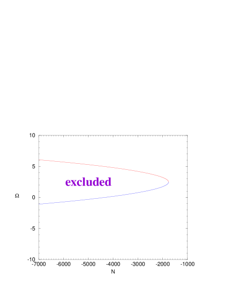
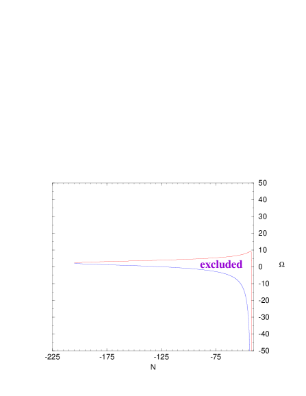
Fig. 1: This is a region the coefficient of the nonrenormalizable term (4.3) vanishes for real $m$, where $m=m(\phi)$ and $\mathchar 28938\relax=\mathchar 28938\relax(\phi)$ are defined as $\frac{B}{\phi B^{\prime}}\equiv\frac{1}{m+2}\mathchar 28938\relax$, $\frac{BB^{\prime\prime}}{B^{\prime 2}}\equiv\frac{m+1}{m+2}\mathchar 28938\relax$. An interesting example is $B=\mbox{constant}\;\phi^{m+2}$ ($m$ is constant of $\phi$). This is the case in Ref [7]. For an arbitrary value of $\phi$, $\mathchar 28938\relax=1$ and some definite value of $m$, this model has no $R^{2}$ term if $N<0$.

References

• [1] M. B. Green, J. H. Schwarz and E. Witten, Superstring Theory, (Cambridge University Press, Cambridge, 1987).
• [2] K. S. Stelle, Renormalization of the Higher Derivative Quantum Gravity, Phys. Rev. 16D, (1977), 953.
• [3] I. L. Buchbinder, S. D. Odintsov and I. L. Shapiro, Effective Action in Quantum Gravity, (IOP, Bristol, 1992).
• [4] G. t’Hooft and M. Veltman, One Loop Divergences in the Theory of Gravitation, Ann. Inst. H. Poincare. A20, 69, (1974).
• [5] S. Christensen and M. Duff, Quantum Gravity with A Cosmological Constant, Nucl. Phys. 170B, (1980), 480.
• [6] A. O. Barvinski, A. Kamenschik and B. Karmazin, The Renormalization Group for Non-Renormalizable Theories: Einstein gravity with A Scalar Field, Phys. Rev. D48, 3677, (1993).
• [7] I. L. Shapiro and H. Takata, One Loop Renormalization of the Four-Dimensional Theory for Quantum Dilaton Gravity, Phys. Rev.D52, 2162, (1995).
• [8] I. L. Shapiro and H. Takata, in Preparation.
• [9] H. Takata, 4D Quantum Dilaton Gravity During Inflation and Renormalization at One-Loop, hep-th.9604170, KEK-TH-481, KEK-preprint-96-10, HUPD-9607.
• [10] S. Mukaigawa and H. Takata, hep-th.9605???, KEK-TH-???, KEK-preprint-96-??, HUPD-9609.
• [11] I. L. Shapiro and H. Takata, Conformal Transformation in Gravity, Phys. Lett. B361, (1995), 31.
• [12] L. F. Abbott, The Background Field Method Beyond One Loop, Nucl. Phys. 185B, (1981), 189.
• [13] B. S. DeWitt, Dynamical Theory of Groups and Fields, (Gordon and Breach, NY, 1965).
• [14] A. O. Barvinski and G. A. Vilkovisky, The Generalized Schwinger-DeWitt Technique in Gauge Theories and Quantum Gravity, Phys. Rep. 119, No. 1, (1985), 1.