UPRF 96-464

IFUM-525-FT

March 1996

Beta function and infrared renormalons
in the exact Wilson renormalization group in Yang-Mills theory

M. Bonini$\,{}^{a}$, G. Marchesini$\,{}^{b}$ and M. Simionato$\,{}^{a}$

${}^{a}\,$Dipartimento di Fisica, Università di Parma
and INFN, Gruppo Collegato di Parma, Italy
${}^{b}\,$Dipartimento di Fisica, Università di Milano
and INFN, Sezione di Milano, Italy

Abstract

We discuss the relation between the Gell-Mann-Low beta function and the “flowing couplings” of the Wilsonian action $S_{\Lambda}[\phi]$ of the exact renormalization group (RG) at the scale $\Lambda$. This relation involves the ultraviolet region of $\Lambda$ so that the condition of renormalizability is equivalent to the Callan-Symanzik equation. As an illustration, by using the exact RG formulation, we compute the beta function in Yang-Mills theory to one loop (and to two loops for the scalar case). We also study the infrared (IR) renormalons. This formulation is particularly suited for this study since: $i$) $\Lambda$ plays the rôle of a IR cutoff in Feynman diagrams and non-perturbative effects could be generated as soon as $\Lambda$ becomes small; $ii$) by a systematical resummation of higher order corrections the Wilsonian flowing couplings enter directly into the Feynman diagrams with a scale given by the internal loop momenta; $iii$) these couplings tend to the running coupling at high frequency, they differ at low frequency and remain finite all the way down to zero frequency.

1 Introduction

In renormalization group (RG) there are two different ways to introduce a momentum scale. The first leads to the Gell-Mann-Low beta function and Callan-Symanzik equation, the second to the exact Wilson RG flow. In the first formulation one introduces the scale $\mu$ at which the coupling $g$, mass and wave function normalization are measured or fixed. The fact that physical quantities do not depend on the scale $\mu$ leads to the Gell-Mann-Low beta function and the Callan-Symanzik equation. In this formulation one does not usually attribute any meaning to the bare action. In the Wilson RG formulation [1] instead the starting point is the local bare action $S_{\Lambda_{0}}[\phi]$ in which the fields $\phi$ have frequencies smaller than the ultraviolet (UV) scale $\Lambda_{0}$. The UV action can be viewed as the result of taking a more elementary theory and integrating all fields with frequencies larger than $\Lambda_{0}$. This gives the coefficients of $S_{\Lambda_{0}}[\phi]$ such as the wave function normalizations $Z_{i}(\Lambda_{0})$ and the parameters $\rho_{i}(\Lambda_{0})$. By further integrating the fields with frequence larger than $\Lambda<\Lambda_{0}$ one obtains a new action $S_{\Lambda}[\phi]$ which is not any more local. This Wilsonian action, and in particular the coefficients $\rho_{i}(\Lambda)$ and $Z_{i}(\Lambda)$ of its local part, the “relevant parameters”, depends on $\Lambda$ according to the exact RG equation [1]-[4]. The physical observables are obtained by performing the path integration over all fields with momenta in the full range $0<q^{2}<\Lambda^{2}_{0}$. Therefore for $\Lambda=0$ (and $\Lambda_{0}\to\infty$) the Wilsonian action generates the physical Green functions. In particular for the wave function normalization one has $Z_{i}(0)=1$ and the parameters $\rho_{i}(0)$ are given by the masses and physical coupling $g$ (at the scale $\mu$).

In this paper we establish the relation between the two RG formulations. We analyze, as examples, the cases of the massless scalar and the $SU(2)$ Yang-Mills theories. To stress the difference on the way the scale is introduced, hereafter we shall call $\mu$-RG and $\Lambda$-RG the first and the second formulation.

First we deduce the Gell-Mann-Low beta function in terms of the derivative of the relevant parameters $\rho_{i}(\Lambda)$ and $Z_{i}(\Lambda)$ of the Wilsonian action. Since RG is related to the UV properties, as expected, this relation involves the UV region of $\Lambda$. Although all perturbative contributions to the relevant parameters diverge logarithmically for large $\Lambda$, in the combination giving the beta function all divergences cancel. It is interesting to observe that in the Yang-Mills case the UV action in general does not satisfy the BRS symmetry and then it could be surprising that the beta function is given in terms of the UV parameters. However one should observe that these UV parameters depend on $g$ and $\mu/\Lambda_{0}$ in such a way that the physical effective action ($\Lambda=0$ and $\Lambda_{0}\to\infty$) satisfies Slavnov-Taylor identities [4, 6].

As a second point concerning the relation between $\mu$-RG and $\Lambda$-RG formulations we show that the Callan-Symanzik equation is equivalent to the condition that the theory is renormalizable, i.e. physical vertices do not depend on the UV scale as $\Lambda_{0}\to\infty$. This is a special case of the $\Lambda$-RG equation which is based on the fact that the physical vertices are obtained from the Wilsonian action $S_{\Lambda}[\phi]$ independently of the value of $\Lambda$.

As a third point we apply the $\Lambda$-RG formulation to the study of infrared (IR) renormalons [7] in non-Abelian gauge theory (and triviality in the scalar theory). IR renormalons could be related to the fact that in a Feynman diagram with a virtual momentum $k$ there are higher order corrections which reconstruct the running coupling $g(k)$ at the scale $k$. Then the momentum integration involves small values of $k^{2}$ where the perturbative running coupling becomes ambiguous and one must include non-perturbative corrections to avoid the IR Landau pole. Although in non-Abelian theories there are various indications supporting this higher order resummations leading to $g(k)$ (non-Abelianization [8] and dispersive methods [9]), no systematic proof of this is known. The $\Lambda$-RG formulation provides a suitable framework in which one can reconstruct the running coupling at large loop momenta and one can study the IR region in Feynman diagrams. The natural couplings in $\Lambda$-RG are the Wilsonian flowing couplings $\hat{g}_{i}(\Lambda)$ given by the relevant parameters $\rho_{i}(\Lambda)$ rescaled by the appropriate wave functions $Z_{j}(\Lambda)$. In the Yang-Mills case there are three Wilsonian couplings $\hat{g}_{i}(\Lambda)$, the relevant coefficients of the three interacting monomials in the classical action (in the scalar case one has a single $\hat{g}(\Lambda)$).

We show that it is possible to set up an iterative procedure to solve the $\Lambda$-RG equations in such a way that one generates contributions of Feynman diagrams in which the loop momenta $k_{i}$ are ordered in virtuality ($k^{2}_{1}<\cdots k^{2}_{\ell}$) and in which the integrands involve the flowing couplings $\hat{g}_{i}(k_{j})$ at these momentum scales. The flowing couplings themselves can be obtained by a generalized beta function which can be computed as an expansion in the Wilsonian coupling itself. We explicitly compare the Wilsonian and the running couplings in the one-loop resummation.

At large scales the running $g(k)$ and the Wilsonian $\hat{g}_{i}(k)$ couplings differ only by $\mu/k$ power corrections. Therefore increasing $k$ all couplings vanish in the Yang-Mills case, while in the scalar case they grow and become singular at the UV Landau pole $k_{L}\simeq\mu\;exp(1/b_{0}g)$ with $b_{0}$ the (positive) one-loop coefficient of the beta function. Therefore also within this $\Lambda$-RG analysis one finds the property of triviality.

For a $k$ comparable to $\mu$ the Wilsonian couplings differ from the running coupling. In the non-Abelian case the one-loop running coupling $g(k)$ diverges at the IR Landau pole and the integration over the small $k$ region become meaningless. In the $\Lambda$-RG formulation instead the Wilsonian couplings $\hat{g}_{i}(k)$ remain finite in all the range of $k$ and at $k=0$ one has $\hat{g}_{i}(0)=g$. Therefore the integration over $k$ is now possible.

In the $\Lambda$-RG formulation $\Lambda$ plays the role of an IR cutoff in Feynman diagrams. So, as long as $\Lambda$ is much larger than $\mu$ one can use the perturbative expressions for the various flowing couplings $\hat{g}_{i}(k_{i})\simeq g(k_{i})$. The Landau singularity is cutoff by the IR scale $\Lambda$ so that non perturbative contributions are negligible and of order $\mu/\Lambda$. For $\Lambda$ approaching the physical point $\Lambda=0$ one has that the various flowing couplings $\hat{g}_{i}(k_{i})$ depart from the running coupling and power corrections resum to make the flowing couplings finite.

The paper is organized as follows. The details of our analysis are presented in Sect. 2 in the case of the massless scalar theory. In Sect. 3 we generalize this analysis to the Yang-Mills theory. Sect. 4 contains some conclusions. In the Appendix we recall the form of the $\Lambda$-RG equations for the scalar case and describe how the usual loop expansion is obtained.

2 Massless scalar case

We illustrate in this case the main elements of the analysis. Some results are general and it is easier to illustrate them in the scalar case. We start by recalling the needed elements of $\Lambda$-RG and then we deduce in this formulation the beta function and compute the two-loop contribution. Then we introduce the improved perturbation expansion in terms of the flowing coupling and compare it with the usual running coupling. All these points will be reanalyzed in the Yang-Mills case in the next section.

2.1 Summary of $\Lambda$-RG formulation

We recall the $\Lambda$-RG formulation by taking as example the euclidean $\phi^{4}$ massless scalar theory in four dimension. One starts from the action at an UV scale $\Lambda_{0}$ larger than any physical scale in the theory

$$S_{\Lambda_{0}}[\phi]=\int d^{4}x\left\{\mbox{\small${{1}\over{2}}$}\phi(x)\;[-Z^{\mbox{\scriptsize UV}}\partial^{2}\;+\;\Lambda_{0}^{2}\;\rho^{\mbox{\scriptsize UV}}_{1}]\;\phi(x)+{{\rho^{\mbox{\scriptsize UV}}_{2}}\over{4!}}\;\phi^{4}(x)\right\}\,.$$ (1)

All fields in the path integrals have frequencies smaller than $\Lambda_{0}$. Thus in Feynman diagrams all internal Euclidean momenta $q_{i}$ are bounded by $q_{i}^{2}\leq\Lambda_{0}^{2}$. The UV parameters $\rho^{\mbox{\scriptsize UV}}_{i}$ are dimensionless. All other possible field monomials have coefficients which are suppressed by inverse powers of $\Lambda_{0}$ since they have negative dimension and here they are neglected for simplicity. Perturbatively this theory is renormalizable so that the UV parameters can be made dependent on $\Lambda_{0}$ in such a way that observables at the physical scales are independent of $\Lambda_{0}$ for $\Lambda_{0}\to\infty$.

The dependence of the UV action on $\Lambda_{0}$ can be generalized to smaller values of the scale. Such a generalization, which is the basis for the $\Lambda$-RG formulation [1], is obtained by performing the path integrations over the fields with frequencies between $\Lambda_{0}$ and $\Lambda<\Lambda_{0}$. This gives the Wilsonian action $S_{\Lambda}[\phi]$ in which the coefficients of the various field monomials depend on $\Lambda$. Of course this action is not any more local.

An equivalent way to obtain the Wilsonian action follows from the observation that $S_{\Lambda}[\phi]$ generates Green functions in which the propagators have both the UV and an IR cutoff $\Lambda$

$$D_{\Lambda\Lambda_{0}}(p)\equiv{{K_{\Lambda\Lambda_{0}}(p)}\over{p^{2}}}\,,$$ (2)

with $K_{\Lambda\Lambda_{0}}(p)=1$ in the region $\Lambda^{2}\leq p^{2}\leq\Lambda^{2}_{0}$ and rapidly vanishing outside. From this property one deduces [1, 2] the RG evolution equation for the Wilsonian action

$$\Lambda\partial_{\Lambda}\;e^{-S_{\Lambda}[\phi]}\;=\;\mbox{\small${{1}\over{2}}$}\int_{q}\;\Lambda\partial_{\Lambda}D_{\Lambda\Lambda_{0}}(q)\;{{\delta^{2}}\over{\delta\phi(q)\delta\phi(-q)}}\;e^{-S_{\Lambda}[\phi]}\,,\;\;\;\;\;\;\;\;\int_{q}\equiv\int{{d^{4}q}\over{(2\pi)^{4}}}\,.$$ (3)

For our study it is convenient to perform the Legendre transform of the Wilsonian action $S_{\Lambda}[\phi]$ and introduce the “cutoff effective action” $\Gamma[\phi;\Lambda,\Lambda_{0}]$ generating the “cutoff vertices” $\Gamma_{2n}(p_{1},\cdots,p_{2n};\Lambda,\Lambda_{0})$. The RG equations for these vertices, corresponding to (3), are schematically given in fig. 1 and they are recalled with the proper details in the Appendix (see [10]-[12]).

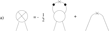
Figure 1: Graphical representation of the $\Lambda$-RG equations for the two point $(a)$ and $2n$-point $(b)$ vertex functions. The black dot represents the full propagator; open circles represent vertex functions with the IR cutoff $\Lambda$; crosses represent the derivative with respect to $\Lambda$ of the free cutoff propagator and vertices. Integration over $q$ in the loop is understood.

The RG equations (3) have to be supplemented by boundary conditions at some values of $\Lambda$. To discuss them one observes that at the UV scale $\Lambda=\Lambda_{0}$ the Wilsonian or cutoff effective action $\Gamma[\phi;\Lambda,\Lambda_{0}]$ reduces to the UV action (1)

$$\Gamma[\phi;\Lambda_{0},\Lambda_{0}]=S_{\Lambda_{0}}[\phi]\,.$$ (4)

Moreover, when the IR and UV cutoff are removed ($\Lambda=0$ and $\Lambda_{0}\to\infty$) and the UV parameters $\rho^{\mbox{\scriptsize UV}}_{i}$ have the proper dependence on $\Lambda_{0}$, the cutoff vertices $\Gamma_{2n}(\{p_{i}\};\Lambda,\Lambda_{0})$ become the physical vertices $\Gamma_{2n}(\{p_{i}\})$

$$\Gamma_{2n}(\{p_{i}\})=\Gamma_{2n}(\{p_{i}\};\Lambda=0,\infty)\,.$$ (5)

The boundary conditions for the RG evolution equations are therefore given by the requirement of locality (4), i.e. by giving the values of the “relevant” UV parameters $\rho^{\mbox{\scriptsize UV}}_{i}$ in (1) and by requiring that all parts of vertices with negative dimension vanish. Without knowing the elementary theory at distances shorter than $1/\Lambda_{0}$, the UV parameters $\rho^{\mbox{\scriptsize UV}}_{i}$ must be obtained from measurement at low scale. To define this procedure one has to introduce in general, for any $\Lambda$, the relevant parameters together with their irrelevant parts.

Relevant parameters, subtraction point and physical couplings. In the four dimensional massless scalar $\phi^{4}$ theory the two and four-point vertices $\Gamma_{2}$ and $\Gamma_{4}$ have non-negative mass dimensions and one has three relevant parameters defined, for instance, as follows

 

$${{}\Gamma_{2}(p;\Lambda,\Lambda_{0})=D^{-1}_{\Lambda\Lambda_{0}}(p)+p^{2}\;(Z(\Lambda)-1)\;+\;\Lambda^{2}\rho_{1}(\Lambda)\;+\;\Delta_{2}(p;\Lambda,\Lambda_{0})\,,}$$

  (6)

with the conditions

$$\Delta_{2}(0;\Lambda,\Lambda_{0})={{d\Delta_{2}(p;\Lambda,\Lambda_{0})}\over{dp^{2}}}|_{p^{2}=\mu^{2}}=0\,,\;\;\;\;\;\;\;\;\Delta_{4}(\bar{p}_{1},\bar{p}_{2},\bar{p}_{3},\bar{p}_{4};\Lambda,\Lambda_{0})=0\,,$$ (7)

where $\mu$ is some subtraction scale and $\bar{p}_{i}$ is the symmetric point $\bar{p}_{i}\bar{p}_{j}=\mu^{2}(\delta_{ij}-{{1}\over{4}})$. At the physical point, from (5) one has

$$Z(0)=1\,,\;\;\;\Lambda^{2}\rho_{1}(\Lambda)|_{\Lambda=0}=0\,,\;\;\;\;\rho_{2}(0)=g\,,$$ (8)

for large $\Lambda_{0}$. These conditions set the field normalization, the mass equal to zero and the coupling at $\mu$.

The relevant parameters at the physical point $\Lambda=0$ are related by the $\Lambda$-RG equations to the UV parameters $\rho^{\mbox{\scriptsize UV}}_{i}$. Therefore as boundary conditions one can take for the relevant parameters the physical values (8) and the vanishing of the irrelevant vertices at the UV point (locality condition (4)). In Appendix we recall how the loop expansion can be generated from the RG equations for the cutoff vertices $\Gamma_{2n}(\{p_{i}\};\Lambda,\Lambda_{0})$ with these boundary conditions.

For the relevant parameters $\rho_{i}(\Lambda)$ and $Z(\Lambda)$ we have explicitly written only the $\Lambda$ dependence. However, from their definition in (6) they are dimensionless functions of $\Lambda$, $\Lambda_{0}$ and $\mu$. One should write $\rho_{i}(\Lambda)\equiv\rho_{i}(g,\mu/\Lambda,\mu/\Lambda_{0})$ and $Z(\Lambda)\equiv Z(g,\mu/\Lambda,\mu/\Lambda_{0})$. In perturbation theory one can take the limit $\Lambda_{0}\to\infty$ and all physical vertices become $\Lambda_{0}$ independent. This implies that one has for large $\Lambda_{0}$

$$\rho_{i}(\Lambda)\;\equiv\;\rho_{i}(g,{\mu}/{\Lambda},{\mu}/{\Lambda_{0}})\;=\;\rho_{i}(g,{\mu}/{\Lambda},0)\;+\;{\cal O}({\mu}/{\Lambda_{0}})\,,$$ (9)

and similarly for $Z(\Lambda)$. This allows one to simplify the perturbative analysis by putting $\Lambda_{0}\to\infty$ from the beginning (see ref. [10]). However, in the scalar $\phi^{4}$ theory, non-perturbative triviality allows one to take this limit only for vanishing $g$.

2.2 Relation between $\Lambda$-RG and $\mu$-RG

As well known renormalization is related to the UV property of the theory. One should then expect that $\mu$-RG , which corresponds to the requirement that the physical observables do not depend on the specific value of $\mu$, is related to $\Lambda$-RG for $\Lambda$ in the UV region. Actually, as we will show, $\mu$-RG corresponds to renormalizability, i.e. the independence of physical vertices on the UV cutoff $\Lambda_{0}$ for large $\Lambda_{0}$. The discussion on this point will be then in the framework of perturbation theory.

From (4) for $\Lambda$ approaching the UV point $\Lambda_{0}$ the cutoff effective action $\Gamma[\phi;\Lambda,\Lambda_{0}]$ becomes the local UV action (1) and one can write

 

$${{}\Gamma[\phi;\Lambda_{0},\Lambda_{0}]=S_{\Lambda_{0}}[\phi]=\int d^{4}x\left\{\mbox{\small${{1}\over{2}}$}\phi^{\mbox{\scriptsize UV}}(x)\;[-\partial^{2}+\Lambda_{0}^{2}\;\bar{\rho}^{\mbox{\scriptsize UV}}_{1}]\;\phi^{\mbox{\scriptsize UV}}(x)\;+\;{{\bar{\rho}^{\mbox{\scriptsize UV}}_{2}}\over{4!}}(\phi^{\mbox{\scriptsize UV}}(x))^{4}\right\}\,,}$$

  (10)

The UV parameters are given by

$$\rho^{\mbox{\scriptsize UV}}_{i}\equiv\rho_{i}(g,{\mu}/{\Lambda},{\mu}/{\Lambda_{0}})|_{\Lambda=\Lambda_{0}}\,,\;\;\;\;Z^{\mbox{\scriptsize UV}}=Z(g,\mu/\Lambda,\mu/\Lambda_{0})|_{\Lambda=\Lambda_{0}}\,.$$ (11)

Consider now the physical vertices $\Gamma_{2n}(\{p_{i}\},g,\mu)$ obtained from this UV action. The rescaling of the fields in (10) allows one to explicitly factorize the dependence on $Z^{\mbox{\scriptsize UV}}$

$$\Gamma_{2n}(\{p_{i}\},g,\mu)=\left(Z^{\mbox{\scriptsize UV}}\right)^{n}\;\Gamma_{2n}^{\mbox{\scriptsize UV}}(\{p_{i}\},\bar{\rho}^{\mbox{\scriptsize UV}}_{1},\bar{\rho}^{\mbox{\scriptsize UV}}_{2};\Lambda_{0})\,.$$ (12)

These UV vertices $\Gamma^{\mbox{\scriptsize UV}}_{2n}$ are obtained from (10) by Feynman rules with internal propagators of momentum $q$ with the UV cutoff $q^{2}<\Lambda_{0}^{2}$. The various Feynman diagram contributions to $\Gamma^{\mbox{\scriptsize UV}}_{2n}$ contain logarithmic divergent powers of

$$\ln\left({{P^{2}}\over{\Lambda^{2}_{0}}}\right)=\ln\left({{P^{2}}\over{\mu^{2}}}\right)+\ln\left({{\mu^{2}}\over{\Lambda_{0}^{2}}}\right)\,,$$ (13)

with $P$ a combination of external momenta. The two point vertex contains also quadratically divergent mass terms proportional to $\Lambda_{0}^{2}$. Renormalizability ensures that (perturbatively) all these $\Lambda_{0}^{2}$ divergences are cancelled by the divergent contributions in the UV parameters $\rho^{\mbox{\scriptsize UV}}_{i}$ and $Z^{\mbox{\scriptsize UV}}$ so that for large $\Lambda_{0}$ the vertex functions are independent of $\Lambda_{0}$. This fact is expressed by the equation

$$\left[\Lambda_{0}\partial_{\Lambda_{0}}+(\Lambda_{0}\partial_{\Lambda_{0}}\bar{\rho}^{\mbox{\scriptsize UV}}_{1}){{\partial}\over{\partial\bar{\rho}^{\mbox{\scriptsize UV}}_{1}}}+(\Lambda_{0}\partial_{\Lambda_{0}}\bar{\rho}^{\mbox{\scriptsize UV}}_{2}){{\partial}\over{\partial\bar{\rho}^{\mbox{\scriptsize UV}}_{3}}}+n\Lambda_{0}\partial_{\Lambda_{0}}\ln Z^{\mbox{\scriptsize UV}}\right]\Gamma_{2n}(\{p_{i}\},g,\mu)=0\,,$$ (14)

valid for large $\Lambda_{0}\to\infty$, i.e. the corrections are of order $\mu/\Lambda_{0}$. Here $\partial_{\Lambda_{0}}$ is the explicit derivative with respect to $\Lambda_{0}$ in (12).

To relate this equation to the $\mu$-RG equation one needs to analyse the $\mu$ dependence of the vertices and then of the UV parameters. The key observation is that, for $\Lambda_{0}\to\infty$, the complete $\mu$ dependence in (12) is contained only in the factor $(Z^{\mbox{\scriptsize UV}})^{n}$. This is due to the fact that the physical vertices $\Gamma_{2n}(\{p_{i}\},g^{\prime},\mu^{\prime})$ with coupling $g^{\prime}$ at a scale $\mu^{\prime}$ are related to the ones with coupling $g$ at $\mu$ by the relation

$$\Gamma_{2n}(\{p_{i}\},g^{\prime},\mu^{\prime})=z^{-n}\;\Gamma_{2n}(\{p_{i}\},g,\mu)\,,\;\;\;\;\;\;z=z(g,{\mu^{\prime}}/{\mu})=Z^{\mbox{\scriptsize UV}}/Z^{\prime{\mbox{\scriptsize UV}}}\,,$$ (15)

with $Z^{\prime{\mbox{\scriptsize UV}}}$ given in (11) as a function of $g^{\prime}$ and $\mu^{\prime}$. Therefore the UV parameters $\bar{\rho}^{\mbox{\scriptsize UV}}_{1}$ and $\bar{\rho}^{\mbox{\scriptsize UV}}_{2}$ become independent of $\mu$ for $\Lambda_{0}\to\infty$. In this limit one obtains the following relation between beta function and UV parameters

$$\beta(g)\equiv\mu\partial_{\mu}g\;=\;{{\Lambda_{0}\partial_{\Lambda_{0}}\,\bar{\rho}^{\mbox{\scriptsize UV}}_{2}}\over{\partial_{g}\,\bar{\rho}^{\mbox{\scriptsize UV}}_{2}}}\;=\;{{\Lambda_{0}\partial_{\Lambda_{0}}\,\bar{\rho}^{\mbox{\scriptsize UV}}_{1}}\over{\partial_{g}\,\bar{\rho}^{\mbox{\scriptsize UV}}_{1}}}\,.$$ (16)

For the field anomalous dimension one has

$$\gamma_{\phi}(g)=-\mbox{\small${{1}\over{2}}$}\mu^{\prime}\partial_{\mu^{\prime}}\;\ln z(g,\mu^{\prime}/\mu)|_{\mu^{\prime}=\mu}=-\mbox{\small${{1}\over{2}}$}[\Lambda_{0}\partial_{\Lambda_{0}}-\beta(g)\partial_{g}]\;\ln Z^{\mbox{\scriptsize UV}}\,.$$ (17)

Notice that the UV parameters are logarithmically divergent for $\Lambda_{0}\to\infty$, but (perturbative) renormalizability ensures that, in this limit, $\beta(g)$ and $\gamma_{\phi}(g)$ are finite and dependent only on $g$.

It is easy to show that the renormalizability condition (14) is equivalent to the $\mu$-RG equation. From (16) and (17) we can write (14) in the form ($\Lambda_{0}\to\infty$)

 

$${{}\left[\Lambda_{0}\partial_{\Lambda_{0}}+\beta(g)\left(\partial_{g}\bar{\rho}^{\mbox{\scriptsize UV}}_{1}{{\partial}\over{\partial\bar{\rho}^{\mbox{\scriptsize UV}}_{1}}}+\partial_{g}\bar{\rho}^{\mbox{\scriptsize UV}}_{2}{{\partial}\over{\partial\bar{\rho}^{\mbox{\scriptsize UV}}_{2}}}+\partial_{g}Z^{\mbox{\scriptsize UV}}{{\partial}\over{\partial Z^{\mbox{\scriptsize UV}}}}\right)-2n\gamma_{\phi}(g)\right]\Gamma_{2n}(\{p_{i}\},g,\mu)}$$

  (18)

From (13) we see the explicit logarithmic $\Lambda_{0}$ dependence is the same as the explicit $\mu$ dependence, thus $\Lambda_{0}\partial_{\Lambda_{0}}$ is equivalent to $\mu\partial_{\mu}$ and one recovers the usual $\mu$-RG equation.

The fact that the theory is (perturbatively) renormalizable ensures that the $\Lambda_{0}$ dependence of the relevant parameters vanishes for $\Lambda_{0}\to\infty$ (see (9)). This implies that we can introduce the relevant parameters $\rho_{i}(g,\mu/\Lambda,\mu/\Lambda_{0})$ directly for $\Lambda_{0}\to\infty$. From now on we shall use

$$\rho_{i}(\Lambda)=\rho_{i}(g,{\mu}/{\Lambda},0)\,,\;\;\;\;Z(\Lambda)=Z(g,{\mu}/{\Lambda},0)\,,$$

so that the beta function in eq. (16) can be expressed in terms of these functions for large $\Lambda$, i.e. $\mu/\Lambda\to 0$. For the beta function and the anomalous dimension one has

 

$${{}\beta(g)=\left[{{\Lambda\partial_{\Lambda}\,\bar{\rho}_{1}}\over{\partial_{g}\,\bar{\rho}_{1}}}\right]_{\mu/\Lambda=0}=\left[{{\Lambda\partial_{\Lambda}\,\bar{\rho}_{2}}\over{\partial_{g}\,\bar{\rho}_{2}}}\right]_{\mu/\Lambda=0}\,,}$$

  (19)

with $\bar{\rho}_{2}=\rho_{2}/Z^{2}$ and $\bar{\rho}_{1}=\rho_{1}/Z$. The parameters $\bar{\rho}_{i}$ have logarithmic divergent contributions for $\mu/\Lambda\to 0$ and only the ratios in (19) are finite. The relation (19) between the beta function and the parameters $\bar{\rho}_{2}$ was obtained in Ref. [5] to one-loop order where the denominator $\partial_{g}\bar{\rho}_{2}$ can be ignored. As we shall see at two loops the denominator is essential to obtain a finite result for $\mu/\Lambda\to 0$.

In the following we shall focus our attention on $\bar{\rho}_{2}$ which will be called the “Wilsonian flowing coupling”, $\hat{g}(\Lambda)\equiv\bar{\rho}_{2}(\Lambda)$. We show now that for large $\Lambda$ this coupling becomes equivalent to a running coupling at the momentum scale $k^{2}=\Lambda^{2}\gg\mu^{2}$. This is a consequence of the fact that for large $\Lambda$ this coupling becomes independent of $\mu$ so that one can write

$$\hat{g}(\Lambda)\equiv\bar{\rho}_{2}(g,\mu/\Lambda)=G(g(\mu),\mu/\Lambda)\;(1\;+\;{\cal O}(\mu/\Lambda))\,,$$

where the function $G$ does not depend on $\mu$. This means that, apart for power corrections, the $\mu$ dependence in $g(\mu)$ is completely cancelled by the explicit $\mu/\Lambda$ dependence. We then can write

$$\hat{g}(\Lambda)=G(g(\Lambda),1)\;(1\;+\;{\cal O}(\mu/\Lambda))\,,\;\;\;\;\;G(g(\Lambda),1)=g(\Lambda)+{\cal O}(g^{2}(\Lambda))\,,$$ (20)

so that $G(g(\Lambda),1)$ itself is a possible running coupling at the scale $\Lambda$.

2.3 Beta function at two loops by $\Lambda$-RG

To illustrate in some details the $\Lambda$-RG formulation we compute the two loop beta function and anomalous dimension using (19) with $\bar{\rho}_{2}$. We have to compute the behaviour for $\mu/\Lambda\to 0$ of the perturbative coefficients of $\rho_{2}$ and $Z$

$$\rho_{2}(g,\mu/\Lambda)=g+\sum_{\ell=1}^{\infty}\;g^{\ell+1}\;\rho^{(\ell)}_{2}(\mu/\Lambda)\,,\;\;\;\;\;Z(g,\mu/\Lambda)=1+\sum_{\ell=2}^{\infty}\;g^{\ell}\;Z^{(\ell)}(\mu/\Lambda)\,.$$ (21)

The corrections to $Z$ start from two loops since the one-loop self energy does not depend on the momentum. The first two coefficients of the beta function

$$\beta(g)=b_{0}g^{2}+b_{1}g^{3}+\cdots$$ (22)

are given by (see (19))

$$b_{0}=\dot{\rho}_{2}^{(1)}|_{\mu=0}\,,\;\;\;\;b_{1}=\;(\,\dot{\rho}_{2}^{(2)}-2\dot{\rho}_{2}^{(1)}\rho_{2}^{(1)}-2\dot{Z}^{(2)}\;)|_{\mu=0}\,,\;\;\;\;\;\dot{\rho}_{i}(\Lambda)\equiv\Lambda\partial_{\Lambda}\rho_{i}(\Lambda)\,.$$ (23)

As we shall see, in the expression for $b_{1}$ the divergence contribution in $\dot{\rho}_{2}^{(2)}$ is cancelled by the divergent contribution $-2\dot{\rho}_{2}^{(1)}\rho_{2}^{(1)}$, which is coming from $\partial_{g}\bar{\rho}_{2}$ in the denominator of (19).

At one loop the relevant parameters are obtained from fig. 1 with the vertices at tree level. The momentum dependence of the self energy vanishes ($Z^{(1)}=0$). Neglecting the subtraction point one finds

$$b_{0}=\dot{\rho}_{2}^{(1)}|_{\mu=0}=-3\int_{q}{{\dot{K}_{\Lambda}(q)}\over{q^{2}}}{{K_{\Lambda}(q)}\over{q^{2}}}=-{{3}\over{2}}\int_{q}{{1}\over{q^{4}}}\Lambda\partial_{\Lambda}K^{2}_{\Lambda}(q)=3r\,,\;\;\;\;\;\;r={{1}\over{16\pi^{2}}}\,.$$ (24)

Notice that since $\dot{\rho}_{2}^{(1)}(\mu/\Lambda)$ is a constant for $\mu/\Lambda=0$, $\rho_{2}^{(1)}(\mu/\Lambda)$ diverges logarithmically as $\ln\mu/\Lambda$.

The two-loop coupling $Z^{(2)}(\mu/\Lambda)$ is obtained from fig. 1a by taking the four point function at one-loop (to this order self energy corrections in internal propagators do not contribute).

Figure 2: Feynman diagram contributing to $\dot{Z}^{(2)}(\Lambda)$.

Neglecting the subtraction point $\mu$ one has (see fig. 2)

$$\dot{Z}^{(2)}|_{\mu=0}=-{{1}\over{6}}\int_{q}\int_{q^{\prime}}\Lambda\partial_{\Lambda}\;\partial_{p^{2}}\left\{{{K_{\Lambda}(q)K_{\Lambda}(q^{\prime})K_{\Lambda}(q+q^{\prime}+p)}\over{q^{2}q^{\prime 2}(q+q^{\prime}+p)^{2}}}\right\}_{p=0}=-{{r^{2}}\over{6}}\,.$$ (25)

These integrals are easily done by neglecting one of the cutoff function. The remaining contribution gives a constant which vanishes when the $\Lambda$-derivative is taken.

The two-loop coupling $\dot{\rho}_{2}^{(2)}(\mu/\Lambda)$ is obtained from the diagrams of fig. 3a, in which the internal vertices are at one loop, and of fig. 3b.

Figure 3: $(a)$ Graphical representation of the contribution to $\dot{\rho}_{2}$ (see the second term of (56)). $(b)$ Feynman diagram contributing to $\dot{\rho}_{2}^{(2)}$ (see the first term of (56)).

The first contribution is

$$g^{3}\dot{\rho}_{2A}^{(2)}|_{\mu=0}=-{{3}\over{2}}\;\int_{q}\left[\Gamma^{2}_{4}(q,0,0,-q;\Lambda)\;\Lambda\partial_{\Lambda}\;{{1}\over{\Gamma^{2}_{2}(q;\Lambda)}}\right]_{\mbox{one loop}}\,.$$ (26)

We have to consider the three contributions $\rho_{1}^{(1)}(\Lambda)$, $\rho_{2}^{(1)}(\Lambda)$ and $\Delta_{4}^{(1)}(q,0,0,-q;\Lambda)$ coming from the one-loop corrections to the two- and four-point functions.

The contribution from $\rho_{1}^{(1)}(\Lambda)$ is zero. This is due to the fact that, before taking the $\Lambda$ derivative, the integral is convergent, dimensionless and then its result is a constant in $\Lambda$.

The contribution from $\rho_{2}^{(1)}(\Lambda)$ is

$$\dot{\rho}_{2A^{\prime}}^{(2)}|_{\mu=0}=-3\;\rho_{2}^{(1)}\;\int_{q}\;\Lambda\partial_{\Lambda}\;\left({{K_{\Lambda}(q)}\over{q^{2}}}\right)^{2}=2\;\rho_{2}^{(1)}\;\dot{\rho}_{2}^{(1)}\,.$$ (27)

As anticipated, this contribution is cancelled by the term $-2\;\rho_{2}^{(1)}\;\dot{\rho}_{2}^{(1)}$ in the combination (23) which is coming from the denominator $\partial_{g}\bar{\rho}_{2}$.

The contribution from $\Delta_{4}^{(1)}(q,0,0,-q;\Lambda)$ is

 

$${\dot{\rho}_{2A^{\prime\prime}}^{(2)}|_{\mu=0}}$$

  (28)

where the equality of the two integrals can be shown by performing the angular integration.

Finally the contribution from the diagram of fig. 3b is

$$\dot{\rho}_{2B}^{(2)}|_{\mu=0}=3\int_{q^{\prime}}\left({{K_{\Lambda}(q^{\prime})}\over{q^{\prime 2}}}\right)^{2}\;\int_{q}\;\Lambda\partial_{\Lambda}\;{{K_{\Lambda}(q)K_{\Lambda}(q+q^{\prime})}\over{q^{2}(q+q^{\prime})^{2}}}\,.$$

It is easy to compute this integral if one of the cutoff functions inside the second integral is neglected

$$\dot{\rho}_{2B^{\prime}}^{(2)}|_{\mu=0}=3\int_{q^{\prime}}\left({{K_{\Lambda}(q^{\prime})}\over{q^{\prime 2}}}\right)^{2}\;\int_{q}\;\Lambda\partial_{\Lambda}\;{{K_{\Lambda}(q)}\over{q^{2}(q+q^{\prime})^{2}}}=-6r^{2}\,.$$ (29)

The remaining term cancels exactly the contribution (28).

In conclusion the only non-cancelling contributions to the two loops beta function and anomalous dimension are given by (25) and (29) and one finds

$$b_{1}=-{{17}\over{3}}r^{2}\,,\;\;\;\;\;\gamma^{(1)}_{\phi}(g)={{1}\over{12}}g^{2}r^{2}\,.$$ (30)

The evaluations given above are obtained essentially by using a theta function for the cutoff function, but the results do not depend on this specific assumption and depend essentially on dimensional counting of convergent integrals. This is due to the fact that one takes the limit $\Lambda\to\infty$ (a smooth representation of the theta function gives corrections vanishing as inverse powers of $\Lambda$).

2.4 Flowing coupling and resummation

As recalled in the Introduction, it is usually assumed that in a Feynman diagram with a virtual loop of momentum $k$ higher order corrections reconstruct the running coupling $g(k)$ at that momentum scale. We want here to show that the $\Lambda$-RG formulation may provide a simple framework in which one can study this resummation.

As we have seen in the previous subsections (see also the Appendix) the usual perturbative expansion is obtained by solving iteratively the $\Lambda$-RG evolution equations with the initial condition that at zero loop the only non vanishing vertices are $\Gamma^{(0)}_{4}(p_{1}\cdots p_{4};\Lambda)=g$ and $\Gamma^{(0)}_{2}(p;\Lambda)=D^{-1}_{\Lambda\Lambda_{0}}(p)$. By iterating the $\Lambda$-RG equations $\ell$ times one generates contributions of Feynman diagrams at $\ell$ loops in which the loop momenta $k_{i}$ are ordered in virtuality $\Lambda^{2}<k^{2}_{1}<\cdots<k^{2}_{\ell}$. The complete Feynman diagrams at that loop are obtained by summing all orderings. This ordering is due to the fact that $\Lambda$ is an IR cutoff $\Lambda^{2}<k_{1}^{2}$ and then in the next iteration $k_{1}^{2}$ plays the rôle of an IR cutoff.

It is possible to formulate an improved iterative procedure in which one introduces the Wilsonian flowing couplings $\hat{g}(k_{i})$ at the scale $k_{i}$ of the successive momenta generated by the iteration. This improved perturbative expansion consists in solving the $\Lambda$-RG equations as for the usual perturbative expansion with the only difference that at zero loop the four point function is given by the flowing coupling

$$\Gamma^{(0)}_{4}(p_{1}\cdots p_{4};\Lambda)=\hat{g}(\Lambda)\,.$$ (31)

The flowing coupling will be obtained later by a generalized beta function computed as an expansion in the Wilsonian coupling itself.

From (31) one starts the iteration by computing to the next loop the irrelevant part of the vertices and the two relevant parameters $Z(\Lambda)$ and $\rho_{1}(\Lambda)$ as function of the flowing coupling. After iterating this procedure $\ell$ times, the vertices are given in terms of flowing couplings $\hat{g}(k_{i})$ at the scale $k_{i}$ of the successive momenta generated by the iteration.

From the vertices obtained after $\ell$ iterations one computes the generalized beta function

$$B[\hat{g};\Lambda]\equiv\Lambda\partial_{\Lambda}\hat{g}(\Lambda)=-2{{\dot{Z}}\over{Z}}\;\hat{g}(\Lambda)+\mbox{\small${{1}\over{2}}$}\;\int_{q}\;Z^{-2}(\Lambda)\;\bar{I}_{6}(q,\bar{p}_{1}\cdots\bar{p}_{4},-q;\Lambda)\;\Lambda\partial_{\Lambda}{{1}\over{\Gamma_{2}(q;\Lambda)}}\,.$$ (32)

The vertex $\bar{I}_{6}$ is defined in the Appendix in terms of the two- four- and six-point cutoff vertices. Solving (32) with the boundary condition $\hat{g}(0)=g$, one computes $\hat{g}(\Lambda)$ as a partial resummation of perturbative expansion. Notice that $B[\hat{g};\Lambda]$ is a functional of the flowing coupling $\hat{g}(k_{i})$ and the scale $\Lambda$. This has to be contrasted with $\beta(g)$ which is a function of $g$.

To illustrate the procedure we compute the flowing coupling to one-loop order (similar approximation has been considered for large $\Lambda$ in Ref. [13]). This is obtained by taking the vertices in the integrand of (32) to zero-loop

$$\bar{I}^{(0)}_{6}(q,p_{1}\cdots p_{4},-q;\Lambda)=-2\hat{g}^{2}(\Lambda)\;\left[D_{\Lambda\Lambda_{0}}(Q_{12})+D_{\Lambda\Lambda_{0}}(Q_{13})+D_{\Lambda\Lambda_{0}}(Q_{14})\right]\,,$$ (33)

where $Q_{ij}=q+p_{i}+p_{j}$. The equation for $Z(\Lambda)$ gives to this order $\dot{Z}^{(1)}(\Lambda)=0$ and one obtains

$$B^{(1)}[\hat{g};\Lambda]=b_{0}\;\hat{g}^{2}(\Lambda)\;f(\mu/\Lambda)\,,$$

where $b_{0}$ is the one-loop coefficient of the beta function and

$$f(\mu/\Lambda)=-8\pi^{2}\int_{q}\;\Lambda\partial_{\Lambda}\;{{K_{\Lambda}(q)\,K_{\Lambda}(q+\bar{p})}\over{q^{2}(q+\bar{p})^{2}}}\;=\;1-{{2\mu}\over{3\pi\Lambda}}+{\cal O}(\mu^{2}/\Lambda^{2})\,,\;\;\;\;\;\Lambda\to\infty\,.$$ (34)

For $\Lambda\to 0$ this function vanishes and one finds $f(\mu/\Lambda)=2(\Lambda/\mu)^{2}+{\cal O}(\Lambda/\mu)^{3}$.

To this order $\hat{g}(\mu/\Lambda)$ is obtained by solving

$$\Lambda\partial_{\Lambda}\hat{g}(\Lambda)=b_{0}\;\hat{g}^{2}(\Lambda)\;f(\mu/\Lambda)\,,\;\;\;\;\;\hat{g}(0)=g\,.$$ (35)

As expected, since $f(\mu/\Lambda)\to 1$ for large $\Lambda$, the flowing and running coupling become the same for large $\Lambda$

$$\hat{g}(\Lambda)={{g}\over{1-b_{0}g\ln(\Lambda/\mu_{0})}}\left(1+{\cal O}({{\mu}\over{\Lambda}})\right)\,,$$ (36)

where $\mu_{0}\simeq\mu$. For smaller $\Lambda$ the two couplings differ: $\hat{g}(0)=g$ while $g(\mu)=g$ and $g(k)\to 0$ for $k\to 0$.

The physical vertices are obtained by integrating the virtualities between $\Lambda=0$ and $\Lambda_{0}$. The presence of the Landau pole at $k_{L}\simeq\mu\,e^{1/b_{0}g}$ implies that the UV cutoff cannot be removed in this case, although the theory is perturbatively renormalizable. This corresponds to the property of triviality of the scalar theory, entailing that the limit $\Lambda_{0}\to\infty$ is possible only if the coupling $g$ vanishes.

3 Yang-Mills case

We show that the previous connection between $\mu$-RG and $\Lambda$-RG formulations can be established also for Yang-Mills theory and we shall compute as an example the one-loop beta function. We recall that the $\Lambda$-RG for this theory is consistent with the BRS symmetry [14] provided the boundary conditions at the physical point $\Lambda=0$ and $\Lambda\to\infty$ are properly chosen [4, 6] (see also [15]). We then consider the iterative solution in terms of the Wilsonian couplings.

3.1 Summary of $\Lambda$-RG formulation

Consider as an example the $SU(2)$ Yang-Mills theory in which $\phi=(A_{\mu}^{a},c^{a},\bar{c}^{a})$ are the vector and the ghost fields and $\gamma=(u_{\mu}^{a},v^{a})$ the sources for composite operators associated to the BRS variations of $A_{\mu}^{a}$, and $c^{a}$ respectively. The BRS classical action, in the Feynman gauge, is

$$S_{\mbox{\footnotesize{BRS}}}=\int d^{4}x\biggl{\{}-{{1}\over{4}}F_{\mu\nu}^{2}-{{1}\over{2}}(\partial_{\mu}A_{\mu})^{2}+W_{\mu}\cdot D_{\mu}c-{{1}\over{2}}\,v\cdot c\wedge c\biggr{\}}\,,$$ (37)

with $F_{\mu\nu}=\partial_{\mu}A_{\nu}-\partial_{\nu}A_{\mu}+gA_{\mu}\wedge A_{\nu}$, $D_{\mu}c=\partial_{\mu}c+gA_{\mu}\wedge c$, $W_{\mu}=\partial_{\mu}\bar{c}+u_{\mu}/g$ and we have introduced the usual scalar and external $SU(2)$ products.

In the $\Lambda$-RG formulation one introduces the cutoff effective action $\Gamma[\phi,\gamma;\Lambda,\Lambda_{0}]$ by using propagators with IR and UV cutoff at $\Lambda$ and $\Lambda_{0}$ respectively and one deduces the RG equation similar to (3). Then one has to fix the boundary conditions. First of all one assumes that at the UV point $\Lambda=\Lambda_{0}$ the cutoff effective action becomes local. Then one has to fix the relevant parameters of $\Gamma[\phi,\gamma;\Lambda,\Lambda_{0}]$, i.e. the coefficients of all independent fields monomials which have dimension not larger than four and are Lorentz and $SU(2)$ scalars. There are nine relevant parameters. Two are the wave function constants $Z_{A}(\Lambda)$ and $Z_{c}(\Lambda)$ for the vector and ghost fields respectively which are the coefficients of the monomials

$$\mbox{\small${{1}\over{2}}$}A_{\mu}(g_{\mu\nu}\partial^{2}-\partial_{\mu}\partial_{\nu})\cdot A_{\nu}\,,\;\;\;\;\;W_{\mu}\cdot\partial_{\mu}\;c\;.$$

The remaining parameters $\rho_{i}(\Lambda)$ with $i=1\cdots 7$ can be taken as the coefficients of the following seven monomials

$$\mbox{\small${{1}\over{2}}$}\Lambda^{2}\,A_{\mu}\cdot A_{\mu}\,,\;\;\;\;-\mbox{\small${{1}\over{2}}$}(\partial_{\mu}A_{\mu})^{2}\,,\;\;\;\;(\partial_{\nu}A_{\mu})\cdot A_{\mu}\wedge A_{\nu}\,,$$

$$W_{\mu}\cdot A_{\mu}\wedge c\,,\;\;\;\;{{1}\over{4}}(A_{\mu}\wedge A_{\nu})\cdot(A_{\nu}\wedge A_{\mu})\,,\;\;\;\;{{1}\over{4}}(A_{\mu}\cdot A_{\mu})^{2}\,,\;\;\;\;-\mbox{\small${{1}\over{2}}$}v\cdot c\wedge c\,,$$

respectively. Notice that some of these monomials are not present in the classical action (37). As in the scalar case (see (6),(7)) these nine parameters are given in terms of vertex functions evaluated at the subtraction points at the scale $\mu$.

At the physical point $\Lambda=0$ and $\Lambda_{0}\to\infty$ the effective action $\Gamma[\phi,\gamma;0,\infty]$ satisfies the BRS symmetry. As shown in Refs. [4, 6] this symmetry is ensured if one properly fixes the relevant parameters defined at a given subtraction point $\mu$ as boundary conditions at $\Lambda=0$. Taking the relevant part of the effective action, i.e. the part which contains only the relevant parameters, one has

$$\Gamma_{\mbox{\footnotesize{rel}}}[\phi,\gamma;0,\infty]=S_{\mbox{\footnotesize{BRS}}}+\hbar\int d^{4}x\biggl{\{}{{x_{5}}\over{4}}(A_{\mu}\wedge A_{\nu})\cdot(A_{\nu}\wedge A_{\mu})+{{x_{6}}\over{4}}(A_{\mu}\cdot A_{\mu})^{2}-\mbox{\small${{1}\over{2}}$}{x_{7}}\,v\cdot c\wedge c\biggr{\}}\,,$$ (38)

where the three parameters $x_{i}$ are given in terms of irrelevant vertices evaluated at the subtraction points (see [6]). Therefore as boundary conditions at the physical point $\Lambda=0$ and $\Lambda_{0}\to\infty$ one assumes

$$Z_{A}(0)=1\,,\;\;\;\;Z_{c}(0)=1\,,\;\;\;\;\rho_{1}(0)=0\,,\;\;\;\;\rho_{2}(0)=1\,,\;\;\;\;\rho_{3}(0)=g\,,\;\;\;\;\rho_{4}(0)=g\,,$$

$$\rho_{5}(0)=g^{2}+\hbar x_{5}\,,\;\;\;\;\rho_{6}(0)=\hbar x_{6}\,,\;\;\;\;\rho_{7}(0)=1+\hbar x_{7}\,.$$

With these conditions the $\Lambda$-RG equation can be solved by expanding in $\hbar$ and one obtains the usual perturbative expansion for the vertex functions which satisfy the Slavnov-Taylor identities.

3.2 Beta function in the $\Lambda$-RG formulation

As in the scalar case we consider the cutoff effective action at the UV point. For $\Lambda=\Lambda_{0}$ the functional $\Gamma[\phi,\gamma;\Lambda,\Lambda_{0}]$ becomes local and equal to the UV action $S_{\Lambda_{0}}[\phi,\gamma]$. As in (11) we introduce the UV wave function constants and UV couplings

$$Z_{i}^{\mbox{\scriptsize UV}}=Z_{i}(g,\mu/\Lambda,\mu/\Lambda_{0})|_{\Lambda=\Lambda_{0}}\,,\;\;\;\;\rho_{i}^{\mbox{\scriptsize UV}}=\rho_{i}(g,\mu/\Lambda,\mu/\Lambda_{0})|_{\Lambda=\Lambda_{0}}\,.$$

Rescaling the fields, the UV action is given by

 

$${{}\Gamma[\phi,\gamma;\Lambda_{0},\Lambda_{0}]=S_{\Lambda_{0}}[\phi,\gamma]}$$

  (39)

where

$$A_{\mu}^{\mbox{\scriptsize UV}}=\sqrt{Z_{A}^{\mbox{\scriptsize UV}}}\;A_{\mu}\,,\quad\quad W^{\mbox{\scriptsize UV}}_{\mu}\,c^{\mbox{\scriptsize UV}}=Z_{c}^{\mbox{\scriptsize UV}}\;W_{\mu}\,c\,.$$ (40)

The UV parameters $\bar{\rho}_{i}^{\mbox{\scriptsize UV}}$ are obtained as in (10) by the usual rescaling. For instance one has

$$\bar{\rho}_{3}^{\mbox{\scriptsize UV}}=\rho_{3}^{\mbox{\scriptsize UV}}\;(Z_{A}^{\mbox{\scriptsize UV}})^{-3/2}\,,\;\;\;\;\;\bar{\rho}_{4}^{\mbox{\scriptsize UV}}=\rho_{4}^{\mbox{\scriptsize UV}}\;(Z_{c}^{\mbox{\scriptsize UV}})^{-1}\;(Z_{A}^{\mbox{\scriptsize UV}})^{-1/2}\,,\;\;\;\;\;\bar{\rho}_{5}^{\mbox{\scriptsize UV}}=\rho_{5}^{\mbox{\scriptsize UV}}\;(Z_{A}^{\mbox{\scriptsize UV}})^{-2}\,.$$

The BRS source $v^{\mbox{\scriptsize UV}}$ is rescaled with no other effect. In the following we consider only vertex functions involving the vector and ghost fields and neglect the $v^{\mbox{\scriptsize UV}}$ source.

The beta function and the field anomalous dimensions are obtained as in the scalar case. After factorizing the UV wave functions (see (12)) the vertices depend only on the six UV parameters $\bar{\rho}_{i}^{\mbox{\scriptsize UV}}$ with $i=1,\cdots 6$. Since the $\mu$ dependence is in the factorized wave function $Z^{\mbox{\scriptsize UV}}_{i}$ one deduces that the six UV rescaled parameters $\bar{\rho}_{i}^{\mbox{\scriptsize UV}}$ do not depend on the subtraction point. Then one finds the relation between the beta function and the UV parameters at $\Lambda_{0}\to\infty$

$$\beta(g)\equiv{{dg}\over{d\ln\mu}}={{\Lambda_{0}\partial_{\Lambda_{0}}\bar{\rho}_{i}^{\mbox{\scriptsize UV}}}\over{\partial_{g}\bar{\rho}_{i}^{\mbox{\scriptsize UV}}}}\,.$$ (41)

Similarly for the field anomalous dimensions one has

$$\gamma_{i}(g)=-\mbox{\small${{1}\over{2}}$}[\Lambda_{0}\partial_{\Lambda_{0}}-\beta(g)\partial_{g}]\ln Z_{i}^{\mbox{\scriptsize UV}}\,.$$ (42)

Due to renormalizability the relevant parameters $\bar{\rho}_{i}(g,\mu/\Lambda,\mu/\Lambda_{0})$ and $Z_{i}(g,\mu/\Lambda,\mu/\Lambda_{0})$ are finite for $\Lambda_{0}\to\infty$. Moreover they diverge for $\Lambda/\mu\to\infty$. Therefore, as in the scalar case, in (41) one can use the parameters $\bar{\rho}_{i}(g,\mu/\Lambda,0)$ and $Z_{i}(g,\mu/\Lambda,0)$ and then take the limit $\mu/\Lambda\to 0$.

The one-loop expression for all the nine parameters has been obtained in [6]

 

$${{}\dot{Z}^{(1)}_{A}|_{\mu=0}={{20}\over{3}}\;r\,,\;\;\;\;\;\;\dot{Z}^{(1)}_{c}|_{\mu=0}=2\;r\,,\;\;\;\;\;\;r\equiv{{1}\over{16\pi^{2}}}\,,}$$

  (43)

According to (41) one finds the well known one-loop beta function ($\beta(g)=b_{0}g^{3}+\cdots$) in the following three ways

$$b_{0}\;=\;(\dot{\rho}_{3}^{(1)}-{{3}\over{2}}\dot{Z}_{A})^{(1)}|_{\mu=0}\;=\;(\dot{\rho}_{4}^{(1)}-\mbox{\small${{1}\over{2}}$}\dot{Z}_{A}^{(1)}-\dot{Z}_{c}^{(1)})|_{\mu=0}\;=\;\mbox{\small${{1}\over{2}}$}(\dot{\rho}_{5}^{(1)}-2\dot{Z}_{A}^{(1)})|_{\mu=0}\;=\;-{{22}\over{3}}\;r\,.$$ (44)

The one-loop beta function cannot be obtained from $\dot{\rho}_{1}^{(1)}$, $\dot{\rho}_{2}^{(1)}$ and $\dot{\rho}_{6}^{(1)}$ since they vanish to this order.

3.3 Flowing couplings and resummation

We extend to the Yang-Mills case the improved perturbation discussed in the scalar case. Here we limit our discussion to the one-loop improved expansion. To this end we have to give the effective action to zero loop (all fields with frequencies between $\Lambda$ and $\Lambda_{0}$)

 

$${{}\Gamma^{(0)}[\phi,\gamma;\Lambda]=\int d^{4}x\biggl{\{}\mbox{\small${{1}\over{2}}$}\;A_{\mu}\cdot\partial^{2}A_{\mu}\;+\;W_{\mu}\cdot\partial_{\mu}c}$$

  (45)

where we have introduced the three flowing couplings

$$\hat{g}_{3A}(\Lambda)=\bar{\rho}_{3}(\Lambda)\,,\;\;\;\;\;\;\hat{g}_{WcA}(\Lambda)=\bar{\rho}_{4}(\Lambda)\,,\;\;\;\;\;\;\hat{g}^{2}_{4A}(\Lambda)=\bar{\rho}_{5}(\Lambda)\,,$$

which are associated to the three field monomials present in the interaction terms of the classical Lagrangian. At one loop no other contribution will be generated (see (43)). At the physical point ($\Lambda=0$ and $\Lambda_{0}\to\infty$) one has

$$\hat{g}_{3A}(0)=\hat{g}_{WcA}(0)=\hat{g}_{4A}(0)=g\,.$$

By iterating the $\Lambda$-RG equation once, for large $\Lambda$ one obtains

 

$${{}{{\dot{Z}_{A}}\over{Z_{A}}}={{19}\over{3}}\;r\;\hat{g}_{3A}^{2}+{{1}\over{3}}\;r\;\hat{g}_{WcA}^{2}\,,}$$

  (46)

and the one-loop generalized beta function

 

$${{}\Lambda\partial_{\Lambda}\hat{g}_{3A}=-{{3}\over{2}}\;{{\dot{Z}_{A}}\over{Z_{A}}}\;\hat{g}_{3A}-{{13r}\over{2}}\hat{g}_{3A}^{3}+{{r}\over{6}}\hat{g}_{WcA}^{3}+9\,r\hat{g}_{3A}\hat{g}_{4A}\,,}$$

  (47)

For $\Lambda$ finite all terms in (46) and (47) have to be multiplied by factors $f_{i}(\mu/\Lambda)$ which are functions similar to $f(\mu/\Lambda)$ in (34) given by integrals over the cutoff functions. These functions vanish quadratically for $\Lambda\to 0$ and they tend to one for $\mu/\Lambda\to 0$, apart for power corrections. Therefore one finds that for large $\Lambda$ the three flowing couplings tend to the one-loop running coupling

$$\hat{g}_{3A}(\Lambda)\simeq\hat{g}_{WcA}(\Lambda)\simeq\hat{g}_{4A}(\Lambda)\simeq g(\Lambda)\,,$$ (48)

with

$$g^{2}(k)={{g^{2}}\over{1-b_{0}\,g^{2}\,\ln(k^{2}/\mu^{2})}}\,\;\;\;\;\;\;b_{0}=-{{22}\over{3}}r\,.$$ (49)

Figure 4: Plot of the one-loop running coupling $\alpha_{s}(\Lambda)$ and the general pattern of the flowing coupling $\hat{\alpha}_{s}(\Lambda)$ in Yang-Mills theory as function of $\Lambda/\mu$. We use $\alpha_{s}(\Lambda)\equiv g^{2}(\Lambda)/4\pi$ and $\hat{\alpha}_{s}(\Lambda)\equiv\hat{g}^{2}(\Lambda)/4\pi$ with $\alpha_{s}(\mu)=\hat{\alpha}_{s}(0)=1$.

As an illustration we consider the case in which all functions $f_{i}(\mu/\Lambda)$ to be included in (46) and (47) are the same and given by the one obtained in the scalar case (34). Then all three coupling are equal ($\hat{g}_{3A}(\Lambda)=\hat{g}_{WcA}(\Lambda)=\hat{g}_{4A}(\Lambda)=\hat{g}(\Lambda)$) and satisfy the RG equation

$$\Lambda\partial_{\Lambda}\hat{g}(\Lambda)=b_{0}\hat{g}^{3}(\Lambda)\;f(\mu/\Lambda)\,,\;\;\;\;\;\;\hat{g}(0)=g\,.$$ (50)

In fig. 4 we plot the solution of this equation together with the corresponding running coupling $g^{2}(\Lambda)$ in (49). For large $\Lambda$ we have $\hat{g}(\Lambda)\simeq g(\Lambda)$. By decreasing the scale the power corrections in $f(\mu/\Lambda)$ start to become important and the two couplings start to differ. The one-loop running coupling has a Landau ghost at $k_{L}^{2}=\mu^{2}\,e^{1/b_{0}g^{2}}<\mu^{2}$. The flowing coupling $\hat{g}(\Lambda)$ instead remains finite in all range of $\Lambda$ and reaches the physical value $g=g(\mu)$ at $\Lambda=0$. Thus in this case, taking $\Lambda=0$, we can compute the physical vertices without problems in the IR integration region.

4 Conclusion

We have studied the relation between $\mu$-RG and $\Lambda$-RG , the formulations of renormalization group based on the two different ways of introducing the momentum scale. While in $\mu$-RG the fundamental quantity is the running coupling $g(k)$ (fixed to be $g$ at $k^{2}=\mu^{2}$), in $\Lambda$-RG the natural couplings are the Wilsonian flowing couplings $\hat{g}_{i}(\Lambda)$ (fixed to be $g$ at $\Lambda=0$).

At large scale $\Lambda=k$ the two couplings differ only by power corrections of $\mu/\Lambda$. This implies that the characteristic quantities of $\mu$-RG formulation are obtained in the $\Lambda$-RG in the UV region of $\Lambda$. In particular the beta function is given by (19) and (41) and is obtained by using the fact that $\hat{g}(\Lambda)$ does not depend on $\mu$ for $\mu/\Lambda\to 0$. Moreover the Callan-Symanzik equation, i.e. independence of $\mu$ of the physical quantities, corresponds to the renormalizability condition, i.e. independence of the UV cutoff $\Lambda_{0}$ of physical quantities for $\Lambda_{0}\to\infty\;$.

An interesting aspect of $\Lambda$-RG formulation is seen in the study of the problem of IR renormalons in non-Abelian gauge theory. We have shown that it is possible to set up an iterative procedure to solve the $\Lambda$-RG equation in such a way that one generates Feynman diagram contributions in which the loop momenta are ordered ($\Lambda^{2}<k_{1}^{2}\cdots<k_{\ell}^{2}$) and the flowing couplings at these momenta are involved. As long as $\Lambda$ is large, one can approximate the flowing couplings in terms of the running coupling. This justifies the usual assumption that in Feynman diagrams with a virtual momentum $k$ higher order corrections generate the running coupling at that scale.

As $\Lambda$ decreases and reaches the physical point $\Lambda=0$ one has to take into account that the flowing couplings differ from the running coupling at low frequencies. At low frequencies, where the perturbative running coupling has a Landau ghost, the flowing couplings are finite all the way down to zero frequence. This allows then to perform the loop integration without problem in the IR region. One should observe that the fact that the flowing couplings are finite in the IR region is due to the presence of power corrections $\mu^{2}/k^{2}$ which are typical non-perturbative contributions.

Acknowledgements

We would like to thank C. Destri for helpful discussions.

5 Appendix

We recall the $\Lambda$-RG equations for the vertex functions in the $\phi^{4}$ massless scalar theory in the form used in the text. The cutoff vertex functions $\Gamma_{2n}(p_{1}\cdots p_{2n};\Lambda,\Lambda_{0})$ have internal propagators

$$D_{\Lambda\Lambda_{0}}(q)={{1}\over{q^{2}}}\;K_{\Lambda\Lambda_{0}}(q)\,,$$ (51)

with $K_{\Lambda\Lambda_{0}}(q)=1$ for $\Lambda^{2}\leq q^{2}\leq\Lambda_{0}$ and rapidly vanishing outside this region.

From the definition of the cutoff vertices and the fact that the $\Lambda$-dependence is only inside the cutoff propagator (51) one deduces [10]-[12] the following $\Lambda$-RG equations (see fig. 1) (we omit to write the $\Lambda_{0}$ dependence in the vertex functions)

$$\dot{\Gamma}_{2}(p;\Lambda)=\dot{D}^{-1}_{\Lambda\Lambda_{0}}(p)-\mbox{\small${{1}\over{2}}$}\int_{q}\;\Gamma_{4}(q,p,-p,-q;\Lambda)\;{{1}\over{\Gamma_{2}^{2}(q;\Lambda)}}\;\dot{D}^{-1}_{\Lambda\Lambda_{0}}(q)\,,$$ (52)

and

$$\dot{\Gamma}_{2n}(p_{1}\cdots p_{2n};\Lambda)=-\mbox{\small${{1}\over{2}}$}\int_{q}\;\bar{\Gamma}_{2n+2}(q,p_{1}\cdots p_{2n},-q;\Lambda)\;{{1}\over{\Gamma_{2}^{2}(q;\Lambda)}}\;\dot{D}^{-1}_{\Lambda\Lambda_{0}}(q)\,,$$ (53)

where the associated vertices $\bar{\Gamma}_{2n+2}$ are one-particle reducible with respect to combinations of momenta including either $q$ or $-q$ and one-particle irreducible with respect to all other combinations of momenta. For instance for $n=3$ one has (we omit the $\Lambda$ and $\Lambda_{0}$ dependence)

$$\bar{\Gamma}_{6}(q,p_{1}\cdots p_{4},-q)=\Gamma_{6}(q,p_{1}\cdots p_{4},-q)\;-\;\sum\Gamma_{4}(q,p_{1},p_{2},Q_{12})\;{{1}\over{\Gamma_{2}(Q_{12})}}\Gamma_{4}(-Q_{12},p_{3},p_{4},-q)$$ (54)

with $Q_{ij}=q+p_{i}+p_{j}$ and the sum is over the six permutations of $p_{1},p_{2},p_{3},p_{4}$. A simpler form for the $\Lambda$-RG equations is obtained by introducing the kernel $I_{2n+2}(q,p_{1}\cdots p_{2n},-q)$ which is one-particle irreducible and also two-particle irreducible with respect to the two momenta $q$ and $-q$. We have then

$$\Gamma_{2n+2}(q\cdots-q)=I_{2n+2}(q\cdots-q)-\mbox{\small${{1}\over{2}}$}\int_{q^{\prime}}\bar{I}_{2n+2}(q^{\prime}\cdots-q^{\prime})\;{{1}\over{\Gamma_{2}^{2}(q^{\prime};\Lambda)}}\;\Gamma_{4}(q,q^{\prime},-q^{\prime},-q)\,,$$ (55)

where, for instance for $n=3$,

$$\bar{I}_{6}(q,p_{1}\cdots p_{4},-q)=I_{6}(q,p_{1}\cdots p_{4},-q)-\sum\Gamma_{4}(q,p_{1},p_{2},Q_{12})\;{{1}\over{\Gamma_{2}(Q_{12})}}\Gamma_{4}(-Q_{12},p_{3},p_{4},-q)\,,$$ (56)

with the sum over the permutations.

From this equation and by using (52) we obtain

$$\dot{\Gamma}_{2}(p;\Lambda)=\dot{D}^{-1}_{\Lambda\Lambda_{0}}(p)+\mbox{\small${{1}\over{2}}$}\int_{q}\,I_{4}(q,p,-p,-q;\Lambda)\;\Lambda\partial_{\Lambda}\;{{1}\over{\Gamma_{2}(q;\Lambda)}}\,,$$ (57)

and

$$\dot{\Gamma}_{2n}(p_{1}\cdots p_{2n};\Lambda)=\mbox{\small${{1}\over{2}}$}\int_{q}\;\bar{I}_{2n+2}(q,p_{1}\cdots p_{2n},-q;\Lambda)\;\Lambda\partial_{\Lambda}\;{{1}\over{\Gamma_{2}(q;\Lambda)}}\,.$$ (58)

In the text we discuss in particular the equations for the relevant parameters $\rho_{1}(\Lambda)$, $\rho_{2}(\Lambda)$ and $Z(\Lambda)$

 

$${{}\Lambda\partial_{\Lambda}(\Lambda^{2}\rho_{1})=\mbox{\small${{1}\over{2}}$}\int_{q}\;I_{4}(q,0,0,-q;\Lambda)\;\Lambda\partial_{\Lambda}\;{{1}\over{\Gamma_{2}(q;\Lambda)}}\,,}$$

  (59)

and

$$\dot{\rho}_{2}=\mbox{\small${{1}\over{2}}$}\int_{q}\;\bar{I}_{6}(q,\bar{p}_{1}\cdots\bar{p}_{4},-q;\Lambda)\;\Lambda\partial_{\Lambda}\;{{1}\over{\Gamma_{2}(q;\Lambda)}}\,,$$ (60)

with $\bar{p}_{i}$ the subtraction point at the scale $\mu$.

The usual loop expansion is obtained by solving iteratively these equations with the initial condition that at zero loop the vertices are given by the two-point function $\Gamma^{(0)}_{2}(p;\Lambda)=D^{-1}_{\Lambda\Lambda_{0}}(p)$ and the four point function $\Gamma^{(0)}_{4}(p_{1}\cdots p_{4};\Lambda)=g$.

References

- [1] K.G. Wilson, Phys. Rev. B 4 (1971) 3174,3184; K.G. Wilson and J.G. Kogut, Phys. Rep. 12 (1974) 75.
- [2] J. Polchinski, Nucl. Phys. B231 (1984) 269.
- [3] G. Gallavotti, Rev. Mod. Phys. 57 (1985) 471.
- [4] C. Becchi, Lectures on the renormalization of gauge theories, in: Relativity, groups and topology II (Les Houches 1983) Eds. B.S. DeWitt and R. Stora (Elsevier Science Pub. 1984); C. Becchi, On the construction of renormalized quantum field theory using renormalization group techniques, in Elementary particles, Field theory and Statistical mechanics, Eds. M. Bonini, G. Marchesini and E. Onofri, Parma University 1993.
- [5] J. Hughes and J. Liu, Nucl. Phys. B307 (1988) 183.
- [6] M. Bonini, M. D’Attanasio and G. Marchesini, Nucl. Phys. B421 (1994) 429, Nucl. Phys. B437 (1995) 163, Phys. Lett. 346B (1995) 87.
- [7] For recent reviews and classical references see V.I. Zakharov, Nucl. Phys. B385 (1992) 452 and A.H. Mueller, in QCD 20 Years Later, vol. 1 (World Scientific, Singapore, 1993).
- [8] M. Beneke and V. Braun, Phys. Lett. 348B (1995) 513 and therein references.
- [9] Yu.L. Dokshitzer, G. Marchesini and B.R. Webber, Dispersive Approach to Power-Behaved Contributions in QCD Hard Processes, hep-ph/9512336, Nucl.Phys to be published.
- [10] M. Bonini, M. D’Attanasio and G. Marchesini, Nucl. Phys. B409 (1993) 441.
- [11] C. Wetterich, Phys. Lett. 301B (1993) 90.
- [12] T.R. Morris, Int. J. Mod. Phys. A9 (1994) 2411.
- [13] S.B. Liao and J. Polonyi, Ann. Phys. (NY) 222 (1993) 122.
- [14] C. Becchi, A. Rouet and R. Stora, Phys. Lett. 52B (1974) 344.
- [15] B.J. Warr, Ann. Phys. (NY) 183 (1988) 1,89; M. Reuter and C. Wetterich, Nucl. Phys. B417 (1994) 181; U. Ellwanger, Phys. Lett. 335B (1994) 364; U. Ellwanger, M. Hirsch and A. Weber, Flow equations for the relevant part of the pure Yang-Mills action, hep-th/9506019.