IASSNS-HEP-95/56

hep-th/9604112

published in Nucl. Phys. B479 (1996) 113

April 1996

Realizing Higher-Level Gauge Symmetries
in String Theory:
New Embeddings for String GUTs
Keith R. Dienes  and  John March-Russell
School of Natural Sciences, Institute for Advanced Study
Olden Lane, Princeton, N.J.  08540  USA

We consider the methods by which higher-level and non-simply laced gauge symmetries can be realized in free-field heterotic string theory. We show that all such realizations have a common underlying feature, namely a dimensional truncation of the charge lattice, and we identify such dimensional truncations with certain irregular embeddings of higher-level and non-simply laced gauge groups within level-one simply-laced gauge groups. This identification allows us to formulate a direct mapping between a given subgroup embedding, and the sorts of GSO constraints that are necessary in order to realize the embedding in string theory. This also allows us to determine a number of useful constraints that generally affect string GUT model-building. For example, most string GUT realizations of higher-level gauge symmetries $G_{k}$ employ the so-called diagonal embeddings $G_{k}\subset G\times G\times...\times G$. We find that there exist interesting alternative embeddings by which such groups can be realized at higher levels, and we derive a complete list of all possibilities for the GUT groups $SU(5)$, $SU(6)$, $SO(10)$, and $E_{6}$ at levels $k=2,3,4$ (and in some cases up to $k=7$). We find that these new embeddings are always more efficient and require less central charge than the diagonal embeddings which have traditionally been employed. As a byproduct, we also prove that it is impossible to realize $SO(10)$ at levels $k>4$. This implies, in particular, that free-field heterotic string models can never give a massless 126 representation of $SO(10)$.

1 Introduction and Overview

1.1 Motivation

As is well-known, the simplest heterotic string constructions lead to models for which the spacetime gauge group $G$ is both simply laced, and realized as an affine Lie algebra with level $k_{G}$ equal to one. While certain level-one simply laced models [1] have met with some phenomenological success, higher-level and/or non-simply laced string models are important from both phenomenological and formal perspectives. It is therefore important to understand the nature of such models, and the common underlying ingredients in their construction.

On the phenomenological side, for example, we may wish to construct string models whose low-energy spectra resemble those of supersymmetric grand-unified theories (SUSY GUT’s). Indeed, such string GUT models represent one possible approach towards explaining the observed unification of gauge couplings within the MSSM. Of course, there exist other attractive string-based approaches towards explaining this unification, such as heavy string threshold corrections [2, 3], non-standard hypercharge normalizations [4], extra matter beyond the MSSM [3, 5], and possible strong-coupling effects [6]. For a recent general review of all of these paths to unification, see Ref. [7].

One advantage of the string GUT approach, however, is that the meeting of the gauge couplings at the MSSM scale $\approx 2\times 10^{16}$ GeV is naturally incorporated. Another advantage is that the GUT idea, at least in the case of $SO(10)$, provides a compelling explanation of the fermion matter content of the Standard Model. One immediate observation that one faces when building string GUT models, however, is that if the massless spectra of such models are to contain the adjoint Higgs representations that are required for the GUT symmetry breaking, then the GUT gauge group must be realized at an affine level $k_{\rm GUT}>1$. Surprisingly, the construction of such higher-level string GUT models has turned out to be a rather complicated affair [8, 9, 10, 11, 12]. It would therefore be useful to have a systematic method of surveying the kinds of higher-level string models that can be constructed, and for analyzing the procedures that would have to be employed for each.

Such higher-level/non-simply laced models are also important from a more formal perspective. Indeed, in some sense, such string models represent generic points in the full string moduli space, and as such they provide a crucial arena for testing some of the predictions of various conjectured string dualities. For example, it has recently been demonstrated that there exist four-dimensional heterotic string models with $N=4$ spacetime supersymmetry whose gauge symmetry groups are non-simply laced [13]. Therefore, unlike simply laced models, such models cannot be self-dual under strong/weak coupling duality ($S$-duality); rather, the predictions of $S$-duality for such models become highly non-trivial, relating such models to each other in a pairwise fashion throughout the moduli space. Finding explicit pairs of such models, however, is an important but as yet unsolved problem.

This paper is devoted towards understanding the general issues that are involved when constructing free-field heterotic string models with higher-level and/or non-simply laced gauge symmetries. As we shall see, the construction of such models is substantially more difficult than that of level-one simply laced string models. Thus, our goal is to develop a more abstract method of understanding how such gauge symmetries generically arise in string theory, and how the possibilities for their construction can be surveyed in an efficient and general manner.

1.2 Our Approach

In this paper, we shall begin an investigation of this general issue by approaching it from one particular, though central, direction. In order to explain our approach, let us first review the basic procedure which underlies the construction of generic string models. This procedure, as we have organized it, is schematically illustrated in Fig. 1.

There are basically three steps in building a heterotic string model; these are illustrated along the left column of Fig. 1. First, one selects a particular string construction (e.g., orbifolds, lattices, free fermions, and so forth). Although each of these constructions contains many free parameters, there are also many string-theoretic self-consistency constraints that must be satisfied: one must maintain conformal invariance, modular invariance, worldsheet supersymmetry, proper spin-statistics relations, physically sensible projections, and so forth. Often these constraints are “built into” the particular string construction from the beginning. For example, in the fermionic approach, there are various rules that govern the allowed choices of fermionic boundary conditions. Likewise, in an orbifold approach, only certain combinations of twists are self-consistent and give rise to sensible models.

Figure 1: Procedures for string model-building, as discussed in the text. Particular choices for the free parameters within a given string construction determine the resulting GSO projections, which in turn define a particular string model. The desired phenomenology, on the other hand, dictates a specific group-theoretic embedding of the gauge and matter representations. The connection between the construction procedure and the desired group-theoretic embedding occurs through the charge lattice, at the level of the GSO projections.

However, even after these self-consistency constraints are satisfied, there typically remain many free parameters (e.g., additional boundary conditions, phases, twists, and so forth) whose values are not yet fixed. The second step in model-building therefore consists of making specific choices for these remaining parameters. Indeed, such specific choices essentially define the string model, and amount to selecting a self-consistent set of GSO projections that will act on the Fock space of string states.

Finally, the third step is to enumerate the states that survive these GSO projections, and thereby determine the physical properties of the model thus constructed. It is in this way that one deduces the final spectrum of the string model, and tests its phenomenological success.

Clearly, many different string models can be generated in this way, and only a small fraction of these will have low-energy features of phenomenological interest. It is therefore important to have some control or guidance over the original choice of free parameters, so that one can efficiently select models with the desired properties.

In the process of string model-building, this phenomenological selection procedure typically occurs through what we can abstractly describe as a two-step process. We have illustrated these two steps along the right column of Fig. 1. First, one starts with a pre-determined set of phenomenological requirements. For example, one may wish to realize a particular gauge group, along with a set of matter representations with specific charge assignments. Then, given these requirements, one determines a preferred group-theoretic embedding. For example, if we wish to construct a string GUT model, we require a GUT gauge group $G_{\rm GUT}$ such as $SU(5)$ or $SO(10)$ along with three complete chiral massless generations and a Higgs scalar transforming in the adjoint of the GUT group. This latter requirement then forces us to realize our GUT gauge symmetry at an affine level $k_{\rm GUT}>1$, and this in turn requires that we choose a special group-theory embedding that is capable of realizing such a higher-level gauge symmetry. A choice that is typically made in the literature is the so-called “diagonal embedding”

$$(G_{\rm GUT})_{2}~{}\subset~{}(G_{\rm GUT})_{1}~{}\times~{}(G_{\rm GUT})_{1}$$ (1.1)

in which the GUT group $G_{\rm GUT}$ is realized at level $k_{\rm GUT}=2$ as the diagonal subgroup of the two-fold tensor product of level-one group factors. This embedding, of course, is only one particular way of realizing such a level-two GUT group, and in general the desired choice of embedding is a subtle issue which must be guided by the desired phenomenology.

Nevertheless, once a specific group-theoretic embedding is chosen, one then makes contact with the three-step string model-construction procedure outlined above at the level of the GSO projections. Specifically, one must choose the GSO projections in such a way as to realize the desired group theory embedding. This is illustrated via the horizontal arrow in Fig. 1. Note that in free-field string constructions (such as those based on free worldsheet bosons or fermions, thereby including all orbifold or lattice constructions), this relation between the GSO projections and the desired embeddings in group theory occurs through the charge lattice. From a string-theoretic standpoint, this charge lattice describes the quantum numbers that string states have under the worldsheet currents that comprise the affine Lie algebra. From a group-theoretic standpoint, however, such lattices are nothing but the root systems or weight systems of the Lie algebra representations. It is therefore here, at the level of the GSO projections and charge lattice, that the connection between the desired phenomenology and a particular string construction occurs, and through which the two can influence each other.

In this paper, we shall focus on this latter connection. In particular, we shall mainly concern ourselves with two broad classes of questions:

• First, given any arbitrary embedding $G^{\prime}_{k^{\prime}}\subset G_{k}$, what are the corresponding GSO projections that will be necessary in order to realize this embedding in string theory? In other words, once a particular embedding is selected, how can this embedding be realized or incorporated into the string framework?

• Second, more generally, what are all of the ways of realizing a given group $G^{\prime}$ at a given level $k^{\prime}$ in free-field string theory? In other words, what are the possible embeddings $G^{\prime}_{k^{\prime}}\subset G_{k}$ that one can ever hope to realize in string theories based on free-field constructions, and what properties do they share? For example, the “diagonal embedding” presented in (1.1) is only one method that gives rise to higher-level GUT groups in string theory. It is natural to wonder whether there might exist other options. Can one find and classify all of the embeddings which can realize GUT groups like $SU(5)$ or $SO(10)$ at higher levels? Might such alternative, non-diagonal embeddings be more efficient than the diagonal embeddings that have been employed up until now?

In this paper, we shall provide explicit answers to all of these questions. Our primary focus will be on those embeddings $G^{\prime}_{k^{\prime}}\subset G_{k}$ for which $G^{\prime}$ is non-simply laced and/or $k^{\prime}>1$ (as these are the more challenging cases), but our treatment will be completely general.

Since our main interest is on this connection between the group-theoretic embeddings and the corresponding GSO projections, there are many other important issues that we will not be discussing in this paper. For example, although we will determine the specific GSO projections that are required in order to realize any arbitrary group-theoretic embedding, we will not approach the issue of whether such GSO projections can be consistently realized within a given string construction (i.e., consistent with modular invariance, spin-statistics constraints, and so forth). In other words, we will not be exploring the connection between the “String Construction” and “GSO Projection” boxes in Fig. 1. While these are important questions, they tend to be highly dependent on the particular string construction employed; indeed, GSO projections that may be simple to realize in one formulation may be impossible to realize in another. Similarly, we will not concern ourselves with the ways in which a particular set of phenomenological requirements influences the selection of a group-theoretic embedding; in terms of Fig. 1, this would be the connection between the “Desired Phenomenology” and “Group Theory Embedding” boxes. Rather, in this paper we will restrict ourselves to analyzing the connection between the possible group-theoretic embeddings, and the GSO projections to which they correspond. Our results will therefore be completely general, and relevant for all model-construction procedures.

1.3 Organization of this paper

This paper is organized in three main parts.

The first part, consisting of Sects. 2–4, develops most of our formal results. In Sect. 2, we provide a brief review of affine Lie algebras, and establish our notation and conventions. Readers familiar with affine Lie algebras are encouraged to skip this section. Then, in Sect. 3, we identify the underlying mechanism by which higher-level and/or non-simply laced gauge symmetries are realized in free-field string constructions. As we shall see, all such realizations correspond to so-called “dimensional truncations” of the charge lattice, and can be analyzed purely in terms of the geometry of such truncations. Finally, in Sect. 4, we present our general formalism, and derive most of our formal results. We find, in particular, that there exists a one-to-one correspondence between consistent dimensional truncations and so-called “irregular” group-theoretic embeddings, and we develop a general procedure for determining the explicit GSO projections that correspond to each such embedding.

The second part of this paper, consisting of Sects. 5 and 6, works through a number of examples of such embeddings and GSO projections, and in the process clarifies several related background issues. Sect. 5, in particular, contains several non-trivial examples of our general results, and Sect. 6 discusses the manner in which the required sorts of GSO projections can be realized in a particular string construction. This analysis will also serve to illustrate how string theory manages to implement an important feature that we shall call the “adjoint to adjoint only” rule. As we shall see, such a rule is ultimately necessary for the consistency of the whole approach.

Finally, in the third part of this paper (Sects. 7 and 8), we apply our general formalism to the study of string GUT embeddings and their corresponding GSO projections. In Sect. 7, we present a complete classification of all embeddings through which the phenomenologically interesting GUT groups $G_{\rm GUT}=SU(5)$, $SU(6)$, $SO(10)$, and $E_{6}$ may be realized in free-field string theory at affine levels $k_{\rm GUT}=2$, 3, and 4. In the case of $SO(10)$, we also extend our results to all levels allowed by naive central-charge constraints, i.e., $k\leq 7$. Since Sect. 7 is rather long and technical, we have collected the results of this classification together in Sect. 7.4, which may be read independently of the rest of this paper. Sect. 8 is then devoted to a detailed analysis of some of the new embeddings and their associated GSO projections.

One of the main results in this part of the paper is an identification of alternative higher-level GUT embeddings which go beyond the simple “diagonal” embeddings in (1.1). As we shall show, some of these alternative embeddings are extraordinarily efficient when compared to the traditional diagonal embeddings, and can be expected to give rise to entirely new classes of potential string GUT models. These alternative embeddings should therefore be of direct importance for string model-builders.

Another important result is a proof that $SO(10)$ can never be realized in free-field heterotic string models at affine levels $k>4$. This implies, for example, that one can never realize the potentially useful massless ${\bf{126}}$ representation of $SO(10)$. This result, like all of our results, is completely general, and holds for all free-field model-construction procedures.

Finally, in Sect. 9, we summarize our main results and discuss various directions for future research. We also discuss how our GUT classification can be used to determine the minimal additional central charge necessary for the string-theoretic realization of GUT gauge symmetries, and therefore the smallest extra chiral algebra that must be generated. Certain technical issues pertaining to our GUT classification in Sect. 7 are then presented in an Appendix.

2 Technical Background: Affine Lie Algebras

In this section, we provide a background review of some basic facts concerning untwisted affine Lie algebras [14], also known as Kač-Moody algebras in the physics literature. This will also serve to establish our definitions and conventions. Readers familiar with affine Lie algebras are encouraged to skip this section.

Affine Lie algebras $\hat{G}$ are infinite-dimensional extensions of the ordinary Lie algebras $G$ that contain this ordinary algebra $G$ as a subalgebra. They are generated by chiral worldsheet currents $J^{a}(z)$ of conformal dimension $(1,0)$ satisfying the operator product expansions (OPE’s)

$$J^{a}(z)J^{b}(w)~{}=~{}{{\tilde{k}}^{ab}\over(z-w)^{2}}~{}+~{}{i\,f^{abc}\over z-w}\,J^{c}(w)~{}+~{}{\rm regular}$$ (2.1)

where $f^{abc}$ are the structure constants of the Lie algebra $G$ (with $a,b,c=1,...,{\rm dim}\,G$), and where the first term on the right side is the “central extension” or Schwinger term. Equivalently, mode-expanding the currents via $J^{a}(z)\equiv\sum_{n\in\mathchoice{\hbox{\cmss Z\kern-3.99994ptZ}}{\hbox{\cmss Z\kern-3.99994ptZ}}{\lower 0.9pt\hbox{\cmsss Z\kern-2.79996ptZ}}{\lower 1.2pt\hbox{\cmsss Z\kern-2.79996ptZ}}}J_{n}^{a}z^{-n-1}$, we find that the OPE (2.1) gives rise to the commutation relations

$$[J^{a}_{m},J^{b}_{n}]~{}=~{}\tilde{k}^{ab}\,m\,\delta_{m+n,0}~{}+~{}i\,f^{abc}\,J^{c}_{m+n}~{}.$$ (2.2)

The subalgebra of modes with $m=n=0$ generates the ordinary Lie algebra $G$, with vanishing central extension.

A basis of currents $J^{a}(z)$ may always be chosen so as to diagonalize the coefficients of the central extension, so that $\tilde{k}^{ab}=\tilde{k}\delta^{ab}$. Furthermore, for a non-abelian group, one can define a unique normalization for the currents $J^{a}(z)$ by fixing a particular normalization for the structure constants. One typically specifies the normalization of the structure constants via

$$\sum_{ab}\,f^{abc}\,f^{abd}~{}=~{}C^{\rm(adj)}_{G}\,\delta^{cd}$$ (2.3)

where $C^{\rm(adj)}_{G}$ is the eigenvalue of the quadratic Casimir acting on the adjoint representation. This then fixes the normalizations of the currents, the value of the central extension coefficient $\tilde{k}$, and the lengths of the root vectors $\{\vec{\alpha}\}$ of the corresponding Lie algebra. Alternatively, one can define the normalization-independent quantities

$$\tilde{h}_{G}~{}\equiv~{}{C^{\rm(adj)}_{G}\over\vec{\alpha_{h}}^{2}}~{},~{}~{}~{}~{}~{}k_{G}~{}\equiv~{}{2\,\tilde{k}\over\vec{\alpha_{h}}^{2}}$$ (2.4)

where $\vec{\alpha}_{h}$ is the longest root. Here $\tilde{h}_{G}$ is the so-called “dual Coxeter number” of the group $G$, and $k_{G}$ is the so-called “level” of the affine Lie algebra. Thus, the level $k_{G}$ of an affine Lie algebra has invariant meaning only for a non-abelian group $G$. In general the dual Coxeter number $\tilde{h}_{G}$ can be calculated for any Lie algebra as

$$\tilde{h}_{G}~{}=~{}{1\over{\rm rank}(G)}\,\left[n_{L}~{}+~{}\left({L\over S}\right)^{-2}n_{S}\right]$$ (2.5)

where $n_{L,S}$ are the numbers of long and short non-zero roots in the root system $\{\vec{\alpha}\}$, and where $L/S$ is the corresponding ratio of their lengths. It turns out that $\tilde{h}_{G}$ is always an integer; likewise, unitarity requires $k_{G}$ to be integral as well. The central charge of the corresponding conformal field theory is:

$$c_{G}~{}=~{}{k\,{\rm dim}(G)\over k+\tilde{h}_{G}}~{}.$$ (2.6)

For each of the classical Lie algebras $G$, the corresponding rank, dimension, root-length ratio, dual Coxeter number, and central charges are tabulated below:

$$G$$ rank() dim()

(2.7)

3 Dimensional Truncations of the Charge Lattice

In this section, we begin by reviewing the subtleties encountered when attempting to realize higher-level or non-simply laced gauge symmetries in string theories based on free-field constructions. We shall then discuss, in a model-independent manner, how these difficulties are ultimately resolved. As we shall see, the resolution involves a special type of GSO projection.

3.1 The Subtleties

It in order to fully appreciate the subtleties that enter the construction of string models with higher-level or non-simply laced gauge symmetries, let us first recall the simplest string constructions — e.g., those based on free worldsheet bosons, or complex worldsheet fermions. In a four-dimensional heterotic string, the conformal anomaly on the left-moving side can be saturated by having $22$ internal bosons $\Phi^{I}$, $I=1,...,22$, or equivalently $22$ complex fermions $\psi^{I}$. If we treat these bosons or fermions indistinguishably, this generates an internal symmetry group $SO(44)$, and we can obtain other internal symmetry groups by distinguishing between these different worldsheet fields (e.g., by giving different toroidal boundary conditions to different fermions $\psi^{I}$). Such internal symmetry groups are then interpreted as the gauge symmetry groups of the effective low-energy theory. Note that in this paper, we are focusing on the gauge symmetries that arise from the left-moving (i.e., internal) degrees of freedom of the heterotic string. If any gauge group arises from the compactified right-moving degrees of freedom, it will appear only via a tensor product with the left-moving gauge group, and will not affect our subsequent analysis.

In general, the spacetime gauge bosons of such left-moving symmetry groups fall into two classes: those of the form $\psi^{\mu}|0\rangle_{R}\otimes i\partial\phi^{I}|0\rangle_{L}$ give rise to the 22 Cartan elements of the gauge symmetry, and those of the form $\psi^{\mu}|0\rangle_{R}\otimes e^{i\alpha\phi_{I}}e^{i\beta\phi_{J}}|0\rangle_{L}$ with $\alpha^{2}+\beta^{2}=2$ give rise to the non-Cartan elements. In the language of complex fermions, both groups of gauge bosons take the simple form $\psi^{\mu}|0\rangle_{R}\otimes\psi^{I}\psi^{J}|0\rangle_{L}$; if $I=J$, we obtain the Cartan elements, whereas if $I\not=J$ we obtain the non-Cartan elements. Together these fill out the adjoint representation of some Lie group. The important point to notice here, however, is the fact that in the fermionic formulation, two fermionic excitations are required on the left-moving side (or equivalently that $\alpha^{2}+\beta^{2}=2$ in the bosonic formulation). Not only is this required in order to produce the two-index tensor representation that contains the adjoint representation (as is particularly evident in the fermionic construction), but precisely this many excitations are also necessary in order for the resulting gauge boson state to be massless.

The next step is to consider the corresponding charge lattice. Each of the left-moving worldsheet bosons $\phi^{I}$ has, associated with it, a left-moving current $J_{I}\equiv i\partial\phi_{I}$ (or in a fermionic formulation, $J_{I}\equiv\overline{\psi}_{I}\psi_{I}$). The eigenvalues $Q_{I}$ of this current when acting on a given state yield the charge of that state. The complete left-moving charge of a given state is a 22-dimensional vector ${\bf Q}$, and the charges of the above gauge boson states together comprise the root system of a rank-22 gauge group (which can be simple or non-simple). However, the properties of this gauge group are highly constrained. For example, the fact that we require two fundamental excitations in order to produce the gauge boson state (or equivalently that $\alpha^{2}+\beta^{2}=2$ in bosonic language) implies that each non-zero root must have (length)${}^{2}=2$. Thus, we see that we can obtain only simply laced gauge groups in such constructions! Moreover, it turns out that in such constructions, the GSO projections only have the power to project a given non-Cartan root into or out of the spectrum. Thus, while we are free to potentially alter the particular gauge group in question via GSO projections, we cannot go beyond the set of rank-22 simply laced gauge groups.

As the final step, let us now consider the affine level at which such groups are ultimately realized. Indeed, this is another property of the gauge group that cannot be altered in such constructions. With fixed normalizations for the currents $J_{a}$ and structure constants $f^{abc}$, we see from (2.1) that

$$k_{G}\cdot|\vec{\alpha}_{h}|^{2}~{}=~{}{\rm constant}~{}=~{}2~{}.$$ (3.1)

Thus, with roots of (length)${}^{2}=2$, we see that our gauge symmetries are realized at level $k_{G}=1$. Indeed, if we wish to realize our gauge group at a higher level (e.g., $k_{G}=2$), then we must somehow devise a special mechanism for obtaining roots of smaller length (e.g., length $=1$). However, as discussed above, this would naively appear to conflict with the masslessness requirement. Thus, on the face of it, it would seem to be impossible to realize higher-level gauge symmetries in string theory.

Note that this problem arises in all constructions based on free worldsheet fields. Indeed, this is because all such constructions automatically give rise to a charge lattice for which the conformal dimensions of the non-Cartan gauge boson states can be identified as $h={\bf Q}^{2}/2$.

3.2 The Resolution

Fortunately, even within free-field constructions, there do exist various methods which are capable of yielding higher-level gauge symmetries. Indeed, although such methods are fairly complicated, they all share certain simple underlying features. We shall now describe, in the language of the above discussion, the general underlying mechanism which enables such symmetries to be realized. It is this general mechanism which ultimately forms the foundation for the rest of this paper.

As we have seen, the fundamental problem that we face is that we need to realize our gauge boson string states as massless states, but with smaller corresponding charge vectors (roots). To do this, let us for the moment imagine that we could somehow project or truncate these roots onto a certain hyperplane in the 22-dimensional charge space, and consider only the surviving components of these roots. Clearly, thanks to this projection, the “effective length” of our roots would be shortened. Indeed, if we cleverly choose the orientation of this hyperplane of projection, we can imagine that our shortened, projected roots could either

• combine with other longer, unprojected roots (i.e., roots which originally lay in the projection hyperplane) to fill out the root system of a non-simply laced gauge group, or

• combine with other similarly shortened roots to fill out the root system of a higher-level gauge symmetry.

Thus, such a projection would be exactly what is required.

The question then arises: how can we achieve or interpret such a hyperplane projection in charge space? Clearly, such a projection would imply that one or more dimensions of the charge lattice should no longer be “counted” towards building the gauge group, or equivalently that one or more of the gauge quantum numbers should be lost. Indeed, such a projection would entail a loss of rank (commonly called “rank-cutting”), which corresponds to a loss of Cartan generators. Thus, we see that we can achieve the required projection if and only if we can somehow construct a special GSO projection which, unlike those described above, is capable of projecting out a Cartan root. This corresponds to a dimensional truncation of the charge lattice.

Indeed, from the above discussions, it is also easy to see this result by proving the reverse statement: without rank-cutting, the only gauge groups that can be realized in free-field string constructions are at level one and must be simply laced. This follows directly as follows. Conformal invariance and masslessness constraints, as we have seen, require that the left-moving vertex operators of gauge-boson states must have conformal dimensions equal to one. In theories without rank-cutting, however, the conformal dimension of a non-Cartan gauge-boson state is related to its 22-dimensional charge vector ${\bf Q}$ via $h={\bf Q}^{2}/2$. We therefore find that such gauge-boson states must always have ${\bf Q}^{2}=2$, which implies that the gauge groups that they produce are necessarily simply laced and realized at level one. This observation is completely general (since it relies on only conformal symmetry and the masslessness constraint), and applies to all free-field heterotic string constructions. Note, in particular, that this argument applies regardless of whether such level-one simply laced groups are realized directly (such as the case of $SO(44)$, for which all gauge bosons arise in the same Neveu-Schwarz sector), or as an enhanced gauge symmetry (such as $E_{8}\times E_{8}\times...$, for which some gauge bosons arise in additional twisted sectors).

Thus, in order to realize a higher-level and/or non-simply laced gauge symmetry in free-field string models, we must start with a level-one simply laced gauge group, and then perform a dimensional truncation of the charge lattice corresponding to that group. As we have said, such dimensional truncations correspond to projecting out Cartan roots from the string spectrum.

What kinds of string constructions can give rise to such unusual GSO projections? As we indicated, such GSO projections cannot arise in simple free-field constructions based on free bosons or complex fermions. Instead, we require highly “twisted” orbifolds (typically asymmetric, non-abelian orbifolds [15]), or constructions based on so-called “necessarily real fermions” [16]. The technology for constructing such string theories is still being developed [8, 9, 10, 11, 17]. For the purposes of this paper, however, the basic point is that such “dimensional truncations” of the charge lattice are the common underlying feature in all free-field constructions of higher-level or non-simply laced string models.

Finally, we comment again on the possibility of gauge symmetries arising from the right-moving (i.e., supersymmetric) worldsheet degrees of freedom of the heterotic string. A consideration of the possible realizations of the worldsheet supercurrent enables one to show that the maximal right-moving gauge symmetry that can arise in this case is $[SU(2)]^{6}$. Furthermore, because the superconformal algebra yields a right-moving vacuum energy of $-1/2$ rather than $-1$, all such states must have ${\bf Q}^{2}_{\rm right}=1$ rather than $2$. Thus, such right-moving gauge symmetries are always realized at affine level two. This is particularly evident in the free-fermionic construction [18], where each potential $SU(2)_{2}$ right-moving gauge-group factor is realized purely in terms of three Majorana-Weyl fermions. Note that such right-moving gauge symmetries are therefore the sole case in which a higher-level gauge symmetry can be realized without a dimensional truncation. In any case, such right-moving gauge symmetries are too small to be of phenomenological interest in the case of string GUT models, and are often entirely absent. They will therefore not concern us further.

3.3 An Example

Before proceeding to a general analysis of such “dimensional truncations”, it is useful to have an explicit example of how they work. Let us therefore consider the well-known method of achieving a level-two symmetry algebra which consists of tensoring together two copies of any group $G$ at level one, and then modding out by the interchange symmetry. This leaves behind the diagonal subgroup $G$ at level two. This construction is well-known in the case $G=E_{8}$, where it serves as the underlying mechanism responsible for the (level-two) $E_{8}$ string model in ten dimensions [20]. For simplicity, let us analyze this construction for the case $G=SU(2)$. If we start with an $SU(2)_{1}^{(A)}\times SU(2)_{1}^{(B)}$ gauge symmetry, as illustrated in Fig. 2, then modding out by the interchange symmetry corresponds to projecting the roots onto the diagonal axis corresponding to the diagonal Cartan generator $J_{z}^{(V)}=J_{z}^{(A)}+J_{z}^{(B)}$. As we can see from Fig. 2, this reproduces the $SU(2)$ root system, but scaled so that roots which formerly had length $\sqrt{2}$ now have length $1$. Thus we realize $SU(2)_{2}$ as the diagonal survivor of the dimensional truncation. In terms of the Cartan generators $U_{1}\equiv J_{z}^{(A)}$ and $U_{2}\equiv J_{z}^{(B)}$ of the original $SU(2)$ factors, it is clear that we simply need project out the linear combination $U_{1}-U_{2}$, retaining the orthogonal combination $U_{1}+U_{2}$. Therefore if we want to realize this particular embedding in string theory, we must construct GSO projections that remove the $|U_{1}\rangle-|U_{2}\rangle$ state, but preserve $|U_{1}\rangle+|U_{2}\rangle$.

By analyzing the root systems in this way — i.e., as dimensional truncations of the charge lattice — we now have a powerful tool at our disposal for determining the possibilities for realizing higher-level and/or non-simply laced gauge symmetries in string theory, and for determining the particular GSO projections to which they correspond. For example, given this simple geometrical interpretation, it is immediately clear that this “diagonal” construction generalizes to any group $G$, for the roots of each level-one gauge factor $G$ always project onto the diagonal hyperplane with a reduction in length by a factor $\cos\,45^{\circ}=1/\sqrt{2}$, causing a doubling of the resulting affine level. Moreover, we also see that this procedure even generalizes to any number $n$ of identical group factors tensored together, $G_{1}\times G_{1}\times...\times G_{1}$, leaving the completely diagonal subgroup $G$ at level $n$.

Figure 2: The root system of $SU(2)_{1}^{(A)}\times SU(2)_{1}^{(B)}$ (denoted by open circles), and its dimensional truncation onto the diagonal subgroup $SU(2)_{2}^{(V)}$ (with new non-zero roots denoted by shaded circles).

However, the vast majority of cases are not this simple. For example, we will see that there exists a method of realizing $SU(2)$ at level $k=4$ which does not involve taking the diagonal tensor product of four copies of $SU(2)$, but which instead realizes $SU(2)_{4}$ as a special subgroup of $SU(3)$ at level $k=1$: $SU(2)_{4}\subset SU(3)_{1}$. An even more dramatic example of a higher-level $SU(2)$ realization is $SU(2)_{10}\subset SO(5)_{1}$. In fact, for even higher levels, the possible embeddings become more and more unexpected. At level 28, for example, it turns out that one can realize $SU(2)_{28}$ not through 28 copies of $SU(2)$, but rather through the single rank-two group $G_{2}$: $SU(2)_{28}\subset G_{2}$. Note that if we wished to realize $SU(2)_{28}$ in string theory, this latter embedding would be crucial, for the “diagonal method” would require that we start with a group of rank at least 28 — too high to be realized in a classical heterotic string.

Clearly, then, for the purposes of string model-building, it is important to have a general way of surveying the possibilities for alternative embeddings, and for determining the GSO projections to which they correspond. For example, if we are interested in building an $SU(5)$ or $SO(10)$ string GUT model, we would like to survey all of the possible methods of realizing $SU(5)_{2}$ or $SO(10)_{2}$ in free-field string constructions. Each different embedding, although yielding the same gauge symmetry, will nevertheless have a drastically different stringy realization, and consequently will correspond to a different low-energy phenomenology. For example, an embedding of the form $SU(10)_{2}\subset SO(10)_{1}\times SO(10)_{1}$ will involve more dimensions of the string charge lattice than an embedding into a smaller-rank group, and will consequently give rise to not only a different “hidden sector” gauge symmetry, but also a different embedding for the matter fields. Such alternate embeddings might be especially useful for tackling the important question of obtaining higher-level GUT gauge symmetries while simultaneously producing three generations.

Furthermore, even after a suitable embedding is chosen, there then remains the separate question of determining the particular GSO projections that will realize this embedding in string theory. For example, let us suppose that we wish to realize the $SU(2)_{10}\subset SO(5)_{1}$ embedding mentioned above. What linear combination of the two Cartan roots $U_{1}$ and $U_{2}$ of the $SO(5)_{1}$ gauge group must then be projected out of the spectrum? (We will answer this question explicitly in Sect. 5.)

Thus, we see that there are two general questions that we would like to answer:

• What are all of the ways of realizing a given group $G$ at a given level $k$ in free-field string constructions?

• In order to realize a particular embedding ${G}^{\prime}_{k^{\prime}}\subset{G}_{k}$, what linear combination of Cartan roots of ${G}_{k}$ must be projected out of the string spectrum?

In the next section, we shall provide general answers to these questions.

4 Irregular Embeddings and GSO Projections

In the previous section, we considered the general process of “dimensional truncation” of the charge lattice, and demonstrated that this is the general underlying mechanism by which higher-level and non-simply laced gauge symmetries are realized in free-field string constructions. In this section, we shall analyze this procedure in a general way. First, given an arbitrary affine Lie algebra $G$, we shall determine the consistent dimensional truncations that may be performed. Then, armed with this knowledge, we will develop a systematic method of determining which Cartan generators of $G$ must be GSO-projected out of the string spectrum in order to explicitly realize each such truncation.

4.1 Regular vs. Irregular Embeddings

We first address the question of determining, for an arbitrary affine Lie algebra $G$, which dimensional truncations are consistent. As we have discovered in the previous section, higher-level and/or non-simply laced gauge symmetries in free-field string constructions are realized only through dimensional truncations of the charge lattices of level-one simply laced groups. Such dimensional truncations correspond to GSO projections which remove one or more Cartan roots from the string spectrum. By contrast, the “ordinary” GSO projections in string theory can delete only various non-Cartan roots, and are therefore capable of producing only level-one, simply laced algebras.

Of course, starting with a level-one simply laced gauge symmetry $G$, it is not necessarily consistent to GSO-project an arbitrary linear combination of Cartan generators out of the spectrum. For example, it is easy to imagine that by removing a poorly-chosen combination of Cartan generators (or equivalently, by projecting onto an improperly oriented hyperplane in charge space), we would wind up with a nonsensical collection of surviving roots that does not correspond to the root system of any Lie algebra at any level, whether simply or non-simply laced. Thus, we must require that any potential dimensional truncation of the adjoint representation of $G$ should yield at least the adjoint representation of some other Lie algebra $G^{\prime}$. However, this is not sufficient. Indeed, we must also demand that the corresponding dimensional truncation of every representation of $G$ produce a representation (not necessarily irreducible) of $G^{\prime}$. Otherwise, the dimensional truncation will produce non-sensical results in other sectors of the theory. Obviously, taken together, these conditions amount to the simple requirement that the final Lie algebra $G^{\prime}$ be a subalgebra of the original Lie algebra $G$.

This much is trivial. However, thanks to our dimensional truncation results of the previous section, we can make some further distinctions. Recall that a group $G$ can have two types of subgroups $G^{\prime}$, often called regular and irregular (or “special”). A subgroup $G^{\prime}$ is called ‘regular’ if its roots are a subset of the roots of the original group $G$. By contrast, an ‘irregular’ subgroup $G^{\prime}$ must necessarily contain some roots which were not present in the original group $G$; in general, such new roots of $G^{\prime}$ are non-trivial linear combinations of the roots of $G$.

This distinction is crucial, because we have seen that dimensional truncations not only reduce rank, but must also truncate at least some of the roots in such a way that these roots are projected onto hyperplanes. Indeed, it was this exactly this projection which gave rise to the required shorter roots with (length)${}^{2}<2$. However, this projection implies that the final (shorter projected) roots that are obtained are necessarily different from the original (longer, unprojected) roots that we started with — i.e., the final set of roots that are obtained are necessarily not a subset of original roots. Thus, we conclude that dimensional truncations necessarily correspond to irregular embeddings. It is therefore only through irregular embeddings that higher-level or non-simply laced gauge symmetries can be realized in free-field string constructions.

This is an important point. Note, in particular, that this does not mean that only irregular embeddings are rank-reducing; indeed, in general a given group will typically contain both regular and irregular subgroups of smaller rank. Thus, both regular and irregular embeddings can correspond to rank-reduction. However, by definition, the roots of regular subgroups always retain the lengths found in the original group. Thus, since the masslessness condition forces us to begin with roots of (length)${}^{2}=2$, we see that regular embeddings are incapable of producing higher-level or non-simply laced gauge groups in such constructions.

It is also an important point that we are making these claims in the physical context of string theory. In particular, there do exist regular embeddings which can give rise to higher-level or non-simply laced gauge groups; two examples of such embeddings are

$$SU(2)_{1}\times SU(2)_{3}~{} \subset ~{}G_{2}~{}$$

$$SU(5)_{2}\times U(1)~{} \subset ~{}Sp(10)_{1}~{}.$$ (4.1)

In the first of these embeddings, the non-zero roots of the $SU(2)_{1}$ gauge factor are taken from the long roots of $G_{2}$, while the non-zero roots of the higher-level $SU(2)_{3}$ gauge factor are taken from the (orthogonal set of) short roots of $G_{2}$. Similarly, in the second case, the 20 non-zero roots of $SU(5)_{2}$ are taken from the short roots of $Sp(10)_{1}$. However, note that both of these embeddings require the presence of non-simply laced gauge groups such as $G_{2}$ or $Sp(10)$ in order to provide us with the short roots we require. As we have seen, such groups can be realized in string theory only through a dimensional truncation procedure of the sort we discussed in Sect. 3. Thus, the realization of higher-level group factors via regular embeddings of the sort (4.1) still requires the existence of an irregular embedding at some prior symmetry-breaking step in the string construction.

4.2 Connecting Irregular Embeddings to Dimensional Truncations: General Formalism

Having made these observations, we now wish to sharpen our connection between irregular embeddings $G^{\prime}_{k^{\prime}}\subset G_{k}$ and dimensional truncations. Note, for example, that our identification of dimensional truncations with irregular embeddings implies that irregular embeddings must somehow be associated with projections in root space. This is indeed the case, and developing the exact connection between the two will enable us to determine which linear combinations of Cartan roots of $G$ must be projected out of the spectrum in order to realize $G^{\prime}$. This will also enable us to geometrically determine the affine level $k^{\prime}$ at which the subalgebra $G^{\prime}$ is realized.

To do this, let us first recall some elementary facts about Lie algebras and their representations. In general, the roots $\{\vec{\alpha}\}$ of a Lie algebra of rank $r$ are vectors in an $r$-dimensional vector space, and among these roots there always exists a special basis of $r$ “simple roots”. Likewise, to each representation of the Lie algebra there corresponds a set of $r$-dimensional vectors (the so-called “weights”) which fill out the representation, and among which there exists a highest weight $\vec{\Lambda}$ from which all others may be obtained by repeated subtractions of the simple roots. In general, a given root or weight $\vec{\Lambda}$ may be specified in a coordinate-independent manner by specifying its Dynkin indices or labels $a_{i}$ with respect to each of the simple roots $\vec{\alpha}_{i}$. These Dynkin indices are defined as

$$a_{i}~{}\equiv~{}{2\,(\vec{\Lambda},\vec{\alpha}_{i})\over(\vec{\alpha}_{i},\vec{\alpha}_{i})}~{}$$ (4.2)

where the inner products between any two roots or weights are evaluated in the (Euclidean) root/weight space. Once these Dynkin indices are known, inner products between any roots or weights can then be determined directly from these indices via the metric tensor $G_{ij}$:

$$(\vec{\Lambda},\vec{\Lambda}^{\prime})~{}=~{}\sum_{ij}\,a_{i}\,G_{ij}\,a^{\prime}_{j}~{}.$$ (4.3)

The metric tensors, highest weights, and Dynkin indices for all of the Lie algebras and their representations can be found, e.g., in Ref. [21]. Finally, we also recall the definition of the so-called quadratic index of a representation of a group $G$ with highest weight $\vec{\Lambda}$:

$$\ell_{G}(\vec{\Lambda})~{}\equiv~{}{{\rm dim}\,R\over{\rm dim}\,G}~{}(\vec{\Lambda},\vec{\Lambda}+2\vec{\delta})~{}=~{}{1\over{\rm rank}\,G}\,\sum_{i=1}^{{\rm dim}\,R}\,(\vec{\lambda}_{i},\vec{\lambda}_{i})~{}.$$ (4.4)

Here $\vec{\delta}$ is defined as half of the sum of the positive roots of $G$, and the $\vec{\lambda}_{i}$ are all of the weights of the representation. In general, $\vec{\delta}$ has Dynkin indices $(1,1,\dots,1)$. The inner products $(\vec{\Lambda},\vec{\Lambda}+2\vec{\delta})$ or $(\vec{\lambda}_{i},\vec{\lambda}_{i})$ are then evaluated as in (4.3).

Given an embedding $G^{\prime}\subset G$, it turns out that there is a simple method for determining the ratio of the corresponding affine levels $k^{\prime}/k$. First, recall that the ratio of the affine levels is given by the ratio of the $({\rm length})^{2}$ of the roots of $G^{\prime}$ and $G$. Next, note that the quadratic index $\ell_{G}$ in (4.4) is directly proportional to this $({\rm length})^{2}$, for the quadratic index scales with the normalization of the root system of $G$. Now, it turns out to be a general feature of irregular embeddings $G^{\prime}\subset G$ that there always exists at least one representation $R^{\ast}$ of $G$ which, under the decomposition $G\to G^{\prime}$, has the simple branching rule $R^{\ast}\to R^{\ast}$. (This will be discussed more fully in Sect. 7.) Thus, for the $R^{\ast}$ representation of $G$, we find that

$${k^{\prime}\over k}~{}=~{}{\ell_{G^{\prime}}(R^{\ast})\over\ell_{G}(R^{\ast})}~{}.$$ (4.5)

Indeed, this result generalizes to any representation $R$ of $G$ as follows. Let us assume that under the decomposition $G\to G^{\prime}$, we have the branching rule $R\to\sum_{i}R_{i}$ where $R_{i}$ are irreducible representations of $G^{\prime}$. Then the so-called embedding index $j(G^{\prime}\subset G)$ of the corresponding irregular embedding $G^{\prime}\subset G$ is defined as [22]

$$j(G^{\prime}\subset G)~{}\equiv~{}{\sum_{i}\ell_{G^{\prime}}(R_{i})\over\ell_{G}(R)}~{},$$ (4.6)

and we have the simple identification

$$k^{\prime}_{G^{\prime}}~{}=~{}j(G^{\prime}\subset G)\,k_{G}~{}.$$ (4.7)

Of course, in (4.6), each of the indices $\ell_{G}(R)$ and $\ell_{G^{\prime}}(R_{i})$ must be computed using the same normalization for the root systems of $G$ and $G^{\prime}$. Note that the identification (4.7) has been previously exploited in the physics literature (see, e.g., [23]).

These results are useful and elegant, but for our purposes in string theory we wish to identify each irregular embedding $G^{\prime}_{k^{\prime}}\subset G_{k}$ with a particular dimensional truncation, for it is only in this geometric way that we will be able to determine which linear combinations of Cartan roots of $G$ need to be GSO-projected out of the spectrum in order to realize the embedding. Thus, we shall now take a slightly different approach, and consider instead the so-called embedding matrix that corresponds to a given subgroup embedding.

Such embedding matrices may be defined as follows. For any given embedding of a subgroup $G^{\prime}$ of rank $r^{\prime}$ within a group $G$ of rank $r$, the corresponding embedding matrix ${\cal P}(G^{\prime}\subset G)$ is a matrix of dimensionality $r^{\prime}\times r$ which maps the Dynkin labels $(a_{1},...,a_{r})$ of the highest weight of a given representation of $G$ onto the Dynkin labels $(a^{\prime}_{1},...,a^{\prime}_{r^{\prime}})$ of the highest weight of the corresponding (not necessarily irreducible) representation of $G^{\prime}$:

$${\vec{a}^{\prime}}~{}=~{}{\cal P}(G^{\prime}\subset G)\,{\vec{a}}~{}.$$ (4.8)

The reduction in rank which necessarily accompanies irregular embeddings implies that the embedding matrix $\cal P$ will not be square in such cases. However, by providing a complete mapping between the representations of $G$ and the corresponding representations of $G^{\prime}$, the embedding matrix $\cal P$ thus succinctly contains all information about the particular embedding of $G^{\prime}$ within $G$, and no further information is required. Thus, given only this embedding matrix ${\cal P}(G^{\prime}\subset G)$, will be able to determine not only which linear combinations of Cartan generators of $G$ must be projected out of the spectrum in order to produce $G^{\prime}$, but also the affine level $k^{\prime}$ at which $G^{\prime}$ will be realized. We shall now give an explicit procedure for carrying out both tasks.

Since we have already determined that irregular embeddings must somehow correspond to dimensional truncations of the charge lattice, our first step must be to determine the orientation of the hyperplane of truncation onto which the roots of the original group must be projected. Now, in general, the orientation of an $r^{\prime}$-dimensional hyperplane passing through the origin within an $r$-dimensional space may be given by specifying $(r-r^{\prime})$ independent $r$-dimensional vectors $\vec{\beta}_{i}$, $i=1,...,r-r^{\prime}$, each of which is perpendicular to the hyperplane. Because such vectors $\vec{\beta}_{i}$ are orthogonal to the hyperplane of truncation, they must have vanishing projection onto this hyperplane. Hence, they satisfy

$$\vec{0}~{}=~{}{\cal P}(G^{\prime}\subset G)\,\vec{\beta}_{i}~{}.$$ (4.9)

In other words, from (4.9), we see that such vectors $\vec{\beta}_{i}$ are simply a set of linearly independent vectors which span the nullspace of ${\cal P}$. If desired, we can subject these vectors $\vec{\beta}_{i}$ to a Gram-Schmidt orthogonalization procedure in order to make them mutually orthogonal.

Given these orthogonal vectors $\vec{\beta}_{i}$, it is now straightforward, following the general procedure outlined in Sect. 4, to determine the affine level $k^{\prime}$ of the subgroup. We simply choose an arbitrary weight $\vec{\Lambda}$ in the weight space of $G$, and determine its projection $\vec{\Lambda}^{\prime}$ onto the corresponding hyperplane:

$$\vec{\Lambda}^{\prime}~{}=~{}\vec{\Lambda}~{}-~{}\sum_{i=1}^{r-r^{\prime}}\,{(\vec{\Lambda},\vec{\beta}_{i})\over(\vec{\beta}_{i},\vec{\beta}_{i})}\,\vec{\beta}_{i}~{}.$$ (4.10)

Thus $(\vec{\Lambda}^{\prime},\vec{\beta}_{i})=0$ for all $\vec{\beta}_{i}$. The squared length of this projected vector $\vec{\Lambda}^{\prime}$ is then simply

$$|\vec{\Lambda}^{\prime}|^{2}~{}=~{}(\vec{\Lambda}^{\prime},\vec{\Lambda}^{\prime})~{}=~{}(\vec{\Lambda},\vec{\Lambda})~{}-~{}\sum_{i=0}^{r-r^{\prime}}\,{(\vec{\Lambda},\vec{\beta}_{i})^{2}\over(\vec{\beta}_{i},\vec{\beta}_{i})}~{}.$$ (4.11)

Thus, in order to determine the level $k^{\prime}$ of the subgroup $G^{\prime}$, we simply compare $|\vec{\Lambda}^{\prime}|^{2}$ against the expected length of the weight in the $G^{\prime}$ system to which $\vec{\Lambda}$ corresponds. It is clear, however, that this $G^{\prime}$-weight is nothing but ${\cal P}\vec{\Lambda}$. We thus find that the level $k^{\prime}$ of the subgroup $G^{\prime}$ is related to the level $k$ of the original group $G$ via

$${k^{\prime}\over k}~{}=~{}{({\cal P}\vec{\Lambda},{\cal P}\vec{\Lambda})\over(\vec{\Lambda},\vec{\Lambda})~{}-~{}\sum_{i=0}^{r-r^{\prime}}\,[(\vec{\Lambda},\vec{\beta}_{i})^{2}/(\vec{\beta}_{i},\vec{\beta}_{i})]}~{}.$$ (4.12)

Note that this result is independent of our choice for $\vec{\Lambda}$, as well as the normalizations of any of the vectors $\vec{\beta}_{i}$. This result does depend, however, upon the overall normalization for ${\cal P}$ being chosen appropriately for similarly normalized roots. In other words, the embedding matrix ${\cal P}$ should map the Dynkin labels $\{a_{i}\}$ of any $G$-weight onto the Dynkin labels $\{a^{\prime}_{i}\}$ of the corresponding $G^{\prime}$-weight, where all of these Dynkin labels $a_{i}$ are to be evaluated, as in (4.2), relative to the identically normalized roots $\vec{\alpha}_{i}$ of the corresponding groups.

We therefore now have two (ultimately equivalent) methods of calculating the affine level of an irregularly embedded subgroup: we can calculate either the “embedding indices” of (4.6), or the general expression in (4.12). Which is easier depends on the information available. In particular, while the embedding indices are often tabulated in mathematical references, the formulation (4.12) is more geometrical, and relies only on the embedding matrix ${\cal P}(G\subset G^{\prime})$. Such an embedding matrix ${\cal P}(G\subset G^{\prime})$ not only contains all information concerning the embedding in question, but is also intimately related to the GSO projections that must be performed in order to realize the embedding.

We now turn, therefore, to the remaining task: the determination of the appropriate linear combinations of Cartan generators of $G$ that must be projected out of the spectrum in order to realize the general embedding $G^{\prime}_{k^{\prime}}\subset G_{1}$. Once again, however, the vectors $\vec{\beta}_{i}$ are precisely what we want, for each corresponds uniquely to a different linear combination of Cartan generators of $G$ that must be GSO projected out of the string spectrum in order to realize $G^{\prime}$. In particular, let $G$ and $G^{\prime}$ have rank $r$ and $r^{\prime}$ respectively, so that the nullspace of ${\cal P}$ is $(r-r^{\prime})$-dimensional, and is spanned by $r-r^{\prime}$ different vectors $\vec{\beta}_{i}$. Also let $U_{\ell}$ ($\ell=1,...,R$) be the Cartan generators of $G$, such that each different generator $U_{\ell}$ corresponds to a different (orthogonal) lattice direction $\hat{e}_{\ell}$ in the root space of $G$. Of course, strictly speaking we have $R=r$, but at this point we leave open the possibility that $R$ may exceed $r$ due to the presence of extra group factors (such as extra $U(1)$ factors) that may arise along with $G$. In other words, we allow for the possibility that the $r$-dimensional root space of $G$ may ultimately be non-trivially embedded within an even larger $R$-dimensional lattice whose directions correspond to an increased number of Cartan generators $U_{\ell}$ ($\ell=1,...,R)$. Then, if the Cartesian (lattice) components of each vector $\vec{\beta}_{i}$ are given by $b^{(i)}_{\ell}$, it follows that the $r-r^{\prime}$ different linear combinations of $U_{\ell}$ which must be projected from the string spectrum are simply given by

$$\sum_{\ell=1}^{R}\,b^{(i)}_{\ell}\,U_{\ell}~{},~{}~{}~{}~{}~{}i=1,...,r-r^{\prime}~{}.$$ (4.13)

Thus, given the $\vec{\beta}_{i}$ vectors as specified by their Dynkin indices, we must first determine their Cartesian coordinates $b^{(i)}_{\ell}$. A priori, this can be done straightforwardly: if a given vector $\vec{\beta}$ in the root space of $G$ has Dynkin labels $a_{j}$ ($j=1,...,r$), then its corresponding Cartesian coordinates $b_{\ell}$ ($\ell=1,...,R$) are given by:

$$b_{\ell}~{}=~{}(\vec{\beta},\hat{e}_{\ell})~{}=~{}\sum_{j,k=1}^{r}\,{4\,(\vec{\beta},\vec{\alpha}_{j})\,G_{jk}\,(\vec{\alpha}_{k},\hat{e}_{\ell})\over|\vec{\alpha}_{j}|^{2}\,|\vec{\alpha}_{k}|^{2}}~{}=~{}\sum_{j,k=1}^{r}\,a_{j}\,{2\,G_{jk}\over|\vec{\alpha}_{k}|^{2}}\,(\vec{\alpha}_{k},\hat{e}_{\ell})$$ (4.14)

where $G_{jk}$ is the metric tensor in root space, and where we have used the definition (4.2). Thus, we see that we must first determine the inner products $(\vec{\alpha}_{k},\hat{e}_{\ell})$. It is here, however, that an important subtlety arises, for we see that we must first determine the relative orientation of the simple roots with respect to the underlying Cartesian coordinate system. In other words, we must determine the ultimate orientation of the charge lattice in terms of the underlying string degrees of freedom. For example, in a string formulation based upon complex worldsheet bosons or fermions, each lattice direction $\hat{e}_{\ell}$ — and consequently each generator $U_{\ell}$ — will correspond to a different boson or fermion: $U_{\ell}\equiv i\partial\phi_{\ell}=\overline{\psi}_{\ell}\psi_{\ell}$. Given such a construction, it is therefore necessary to determine the orientation or embedding of the simple roots of the gauge group $G$ with respect to these lattice directions.

Fortunately, this can be determined by recalling how such (simply laced) gauge groups $G$ are ultimately realized in free-field string constructions. In particular, the gauge boson states in string theory are always realized in terms of simple particle and anti-particle excitations of the underlying worldsheet fields. We shall see an explicit example of this in Sect. 6.2. Thus, we see that the appropriate realization of the roots of $G$ is essentially fixed (up to irrelevant overall lattice permutations and inversions) in terms of the lattice directions $\hat{e}_{\ell}$. For example, in the case of $SO(2r)$, the roots $\{\vec{\alpha}\}$ are given as $\{\pm\hat{e}_{i}\pm\hat{e}_{j}\}$, with the simple roots given by $\vec{\alpha}_{i}=\hat{e}_{i}-\hat{e}_{i+1}$ for $i\leq r-1$, and $\vec{\alpha}_{r}=\hat{e}_{r-1}+\hat{e}_{r}$. Given such an explicit realization, the relative orientation of the simple roots with respect to the Cartesian coordinate system is then fixed. For convenience, we now list the appropriate inner products $(\vec{\alpha}_{i},\hat{e}_{\ell})$ for each of the classical Lie groups:

$$SU(r+1): (\vec{\alpha}_{k},\hat{e}_{\ell})~{}=~{}\phantom{\bigl{\{}}\delta_{k,\ell}-\delta_{k+1,\ell}~{}~{}~{}~{}{\rm for~{}all}~{}1\leq k\leq r$$

$$SO(2r+1): (\vec{\alpha}_{k},\hat{e}_{\ell})~{}=~{}\cases{\delta_{k,\ell}-\delta_{k+1,\ell}&if $1\leq k<r$\cr\delta_{r,\ell}&if $k=r$\cr}$$

$$Sp(2r): (\vec{\alpha}_{k},\hat{e}_{\ell})~{}=~{}\cases{(\delta_{k,\ell}-\delta_{k+1,\ell})/\sqrt{2}&if $1\leq k<r$\cr\sqrt{2}\,\delta_{r,\ell}&if $k=r$\cr}$$

$$SO(2r): (\vec{\alpha}_{k},\hat{e}_{\ell})~{}=~{}\cases{\delta_{k,\ell}-\delta_{k+1,\ell}&if $1\leq k<r$\cr\delta_{r-1,\ell}+\delta_{r,\ell}&if $k=r$\cr}$$ (4.15)

As required, in each case we have normalized the simple roots so that the long roots have length $\sqrt{2}$. The inner products in (4.15) can then be substituted into (4.14) and (4.13) in order to determine which linear combinations of Cartan generators must be projected out of the string spectrum.

Note that, in general, the $SU(n)$ groups are realized in string theory by first realizing $U(n)\equiv SU(n)\times U(1)$ in an $n$-dimensional lattice. In this $n$-dimensional lattice, the $U(1)$ group factor amounts to the trace of the $U(n)$ symmetry, and corresponds to the lattice direction ${\bf E}\equiv\sum_{\ell=1}^{n}\hat{e}_{\ell}$. The $(n-1)$-dimensional hyperplane orthogonal to ${\bf E}$ then corresponds to the $SU(n)$ gauge group. This explains why, as in (4.15), the number of required lattice directions $\hat{e}_{\ell}$ for the $SU(r+1)$ case is larger than the rank of the group. Thus, if $r$ is the rank of the group $G$ in (4.13) and if $R$ is the corresponding number of required string lattice directions, we find that we can have $R=r$ for the $G=SO$ and $Sp$ groups, but require $R=r+1$ for the $SU$ groups.

Thus, through the general procedure outlined in this section, we see that we have succeeded in identifying every irregular embedding with a particular geometric dimensional truncation in root space. Indeed, for every irregular embedding $G^{\prime}_{k^{\prime}}\subset G_{k}$, we now know precisely the dimensional truncation to which it corresponds, and the particular GSO projections of Cartan generators that are required to achieve it. Thus, in a general fashion, we find that have completely described the underlying mechanism which is responsible for the generation of higher-level and/or non-simply laced gauge symmetries in free-field string constructions. In the remainder of this paper, we shall consider various extensions and applications of these general results.

5 Examples

In this section we shall give two explicit examples of the general results of Sect. 4. We shall choose two particular irregular embeddings, and show how each corresponds to precisely a dimensional truncation of the sort that arises in an actual string-theoretic construction. We will also determine the affine levels of the subgroups, and deduce the GSO projections that are required in order to realize these particular embeddings.

5.1 First Example: $SU(2)_{4}\subset SU(3)_{1}$

Perhaps the simplest case to consider is the irregular embedding of $SU(2)$ within $SU(3)$. Since this is an irregular embedding, the roots of $SU(2)$ are not a subset of the roots of $SU(3)$, and in particular the Cartan generator of $SU(2)$ is neither of the Cartan generators of $SU(3)$. Rather, the three generators $J_{x,y,z}$ of this irregularly-embedded $SU(2)$ are realized as linear combinations of the non-Cartan generators of $SU(3)$:

$$J_{x}~{}\equiv -\sqrt{2}\,i\,(V_{+}-V_{-}) =~{}2\,F^{7}$$

$$J_{y}~{}\equiv -\sqrt{2}\,i\,(I_{+}-I_{-}) =~{}2\,F^{2}$$

$$J_{z}~{}\equiv -\sqrt{2}\,i\,(U_{+}-U_{-}) =~{}2\,F^{5}$$ (5.1)

Here $\{I_{\pm},U_{\pm},V_{\pm}\}$ are the non-Cartan generators of $SU(3)$ as labelled in Fig. 3, and the $F^{i}$ refer to the $SU(3)$ generators in the Gell-Mann basis. One then easily finds, given the $SU(3)$ commutation relations for $\{I_{\pm},U_{\pm},V_{\pm}\}$, that $\{J_{x},J_{y},J_{z}\}$ satisfy the $SU(2)$ commutation relations. Indeed, we can determine the level of the $SU(2)$ affine Lie algebra by calculating the affinized commutation relations as follows. The $SU(3)$ structure constants $f^{ijk}$ in the Gell-Mann basis are normalized as $\sum_{jk}f^{ijk}f^{\ell jk}=3\delta^{i\ell}=\tilde{h}_{SU(3)}\delta^{i\ell}$, which corresponds to the highest root having length $1$. In particular, $f^{257}=1/2$, and there are no other non-zero structure constants involving any two of these indices. Thus, if the $SU(3)$ group is realized at any arbitrary level $k$, then the corresponding commutation relations between the $F^{2,5,7}$ generators are given by

$$[F^{i}_{m},F^{j}_{n}]~{}=~{}{i}\,f^{ijk}\,F^{k}_{m+n}~{}+~{}{k\over 2}\,m\,\delta^{ij}\,\delta_{m+n,0}~{}$$ (5.2)

and cyclic permutations. Among these generators, the structure constant $f^{ijk}$ will take only the values $\{0,\pm 1/2\}$. From (5.2) we therefore see that

$$[J^{i}_{m},J^{j}_{n}]~{}=~{}{i}\,(2f^{ijk})\,J^{k}_{m+n}~{}+~{}{k^{\prime}\over 2}\,m\,\delta^{ij}\,\delta_{m+n,0}~{}$$ (5.3)

where $k^{\prime}=4k$. Furthermore, the new structure constants $2f^{ijk}$ with $i,j,k=2,5,7$ are nothing but $\epsilon^{ijk}$, the structure constants for $SU(2)$ in a normalization with $SU(2)$ roots having length $1$. We thus identify $k^{\prime}=4k$ as the level of the $SU(2)$ subgroup, so that $SU(2)_{4}\subset SU(3)_{1}$ for this irregular embedding.

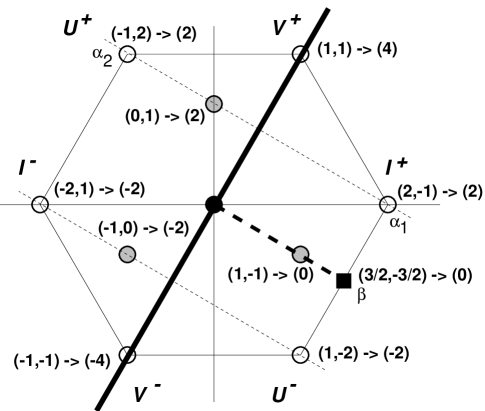
Figure 3: The irregular embedding of $SU(2)_{4}$ within $SU(3)_{1}$. The non-zero roots of $SU(3)_{1}$ lie along the outer hexagon, as denoted by empty circles. The roots labelled $\vec{\alpha}_{1}$ and $\vec{\alpha}_{2}$ are the simple roots, and the weights of the fundamental 3 representation of $SU(3)$ are also shown (shaded circles). Next to each weight we have listed its Dynkin labels, along with the Dynkin label of the $SU(2)$ weight to which it corresponds according to the embedding matrix in Eq. (5.4). The axis of $SU(2)$ truncation is also shown (dark line), with the vector $\vec{\beta}$ (black square) chosen perpendicular to this axis.

This much is standard. However, in order to relate this to the geometrical dimensional truncations of Sect. 3, let us now follow the procedure outlined in Sect. 4 and consider the decompositions of the various $SU(3)$ representations. This irregular embedding is defined by the ${\bf{3}}\to{\bf{3}}$ and ${\bf{8}}\to{\bf{5}}+{\bf{3}}$ branching rules. Now, in general, the Dynkin label of the highest weight of the ${\bf{2j+1}}$ representation of $SU(2)$ is simply $(2j)$, while the Dynkin labels for highest weights of the fundamental and adjoint representations of $SU(3)$ are respectively $(0,1)$ and $(1,1)$. Thus the embedding matrix ${\cal P}$ must map $(0,1)$ to (2), and $(1,1)$ to $(4)$, implying

$${\cal P}(SU(2)\subset SU(3))~{}=~{}\pmatrix{2&2\cr}~{}.$$ (5.4)

Given this, we see from Fig. 3 that for each $SU(3)$ weight, the corresponding $SU(2)$ Dynkin label is proportional to the length of its projection onto the axis indicated. Thus, the irregular $SU(2)\subset SU(3)$ embedding corresponds precisely to the geometrical process of dimensional truncation that we discussed in Sect. 3. Indeed, such an identification would have seemed somewhat mysterious, given only the explicit realization of the subgroup as listed in (5.1). Moreover, just as outlined in Sect. 4, the proportionality factor between the actual length of the projection and the length anticipated from the $SU(2)$ Dynkin label allows us to deduce the level of the subalgebra. Since the $SU(2)$ root system realized through this projection is scaled down by a factor of two, the affine level increases by a factor of $4$, in agreement with the explicit calculation above. Of course, given the six-fold Weyl symmetry of the $SU(3)$ root system, the irregular embedding $SU(2)_{4}\subset SU(3)_{1}$ actually corresponds in general to a dimensional truncation onto any axis which is related to that in Fig. 3 by an element of the Weyl group.

Finally, we now determine which GSO projection is required in order to realize this $SU(2)_{4}\subset SU(3)_{1}$ embedding. The nullspace of the ${\cal P}$-matrix in (5.4) is spanned by the single vector $\vec{\beta}$ whose Dynkin labels are given by $(1,-1)$. Thus, we must first convert these to Cartesian coordinates. Since the original group in this case is an $SU$ group, we cannot simply use the graphical representation given in the figure, for we recall from the previous section that such an $SU(3)$ group, along with an additional orthogonal $U(1)$ group factor, will be realized together in a three-dimensional lattice. Indeed, following the formalism given the previous section, we find that the two simple roots $\vec{\alpha}_{1},\vec{\alpha}_{2}$ of $SU(3)$, as well as the nullspace vector $\vec{\beta}$, will have the following Cartesian coordinates:

$$\vec{\alpha}_{1}~{}=~{}(1,-1,0)~{},~{}~{}~{}~{}~{}~{}~{}\vec{\alpha}_{2}~{}=~{}(0,1,-1)~{},~{}~{}~{}~{}~{}~{}~{}\vec{\beta}~{}=~{}(1,-2,1)~{}.$$ (5.5)

Note that all of these coordinates are rational in this three-dimensional realization; indeed, this is one of the reasons that string theory requires such a three-dimensional space in order to realize $SU(3)_{1}$. Thus, we conclude that if $U_{i}$ are the three Cartan generators that correspond respectively to these three lattice directions, the subsequent $SU(2)_{4}\subset SU(3)_{1}$ embedding can be realized by projecting out the linear combination

$$SU(2)_{4}\subset SU(3)_{1}:~{}~{}~{}~{}~{}~{}{\rm project~{}out}~{}~{}~{}U_{1}-2\,U_{2}+U_{3}~{}.$$ (5.6)

Note that although we required three Cartan generators in order to realize the $SU(3)$ group factor and to express this dimensional truncation, this does not imply that $SU(2)_{4}$ is really embedded in $SU(3)_{1}\times U(1)$. Indeed, the entire dimensional truncation occurs within the two-dimensional subspace that corresponds to $SU(3)$ alone (as illustrated in the figure), and the extra $U(1)$ factor, which corresponds to the Cartan generator $U_{1}+U_{2}+U_{3}$, is truly orthogonal to the entire process. Thus, as claimed, we have truly realized an $SU(2)_{4}\subset SU(3)_{1}$ embedding. Such an embedding is an extremely efficient way of realizing $SU(2)_{4}$ in string theory, for we see that only one lattice dimension must be sacrificed in the process. By contrast, the diagonal embedding $SU(2)_{4}\subset[SU(2)_{1}]^{4}$ would have required the sacrifice of three lattice dimensions.

5.2 Second Example: $SU(2)_{10}\subset SO(5)_{1}$

As a less-trivial example (indeed, one for which the axis of truncation does not correspond to any symmetry axis of the weight diagram), let us examine the irregular embedding of $SU(2)$ within $SO(5)$. This is illustrated in Fig. 4. In this embedding, the 5 and 4 representations [for which the highest weights have Dynkin labels (1,0) and (0,1) respectively] map directly onto the 5 and 4 representations of $SU(2)$ [with respective Dynkin labels (4) and (3) in the $SU(2)$ normalization with roots of $({\rm length})^{2}=2$]. Thus the embedding matrix in this case is given by

$${\cal P}(SU(2)\subset SO(5))~{}=~{}\pmatrix{4&3\cr}~{}.$$ (5.7)

The effects of this embedding matrix on the Dynkin labels of the 4, 5, and 10 representations of $SO(5)$ are shown in the figure.

Given these Dynkin label mappings, it is straightforward to deduce the corresponding orientation of the $SU(2)$ axis of truncation (also shown in the figure). As indicated in the figure, the vector $\vec{\beta}$ with Dynkin labels $(-3/2,2)$ defines the nullspace of ${\cal P}$, and hence defines the orientation of the axis of projection. Given this orientation, we immediately see that the 5 representation of $SO(5)$ fills out the $j=2$ representation of $SU(2)$, and that the 4 representation fills out the $j=3/2$ representation. The full adjoint representation of $SO(5)$ likewise decomposes into the ${\bf{7}}+{\bf{3}}$ representations of $SU(2)$.

To determine the level of the $SU(2)$ subgroup, we can calculate, for example, the length of the projection of the simple root $\vec{\alpha}_{2}$ onto the $SU(2)$ axis. This is most easily done by first determining the angle $\theta$ between $\vec{\alpha}_{2}$ and $\vec{\beta}$, as follows. Clearly the length $|\vec{\alpha}_{2}|$ is $1$, and we can determine the length of $\vec{\beta}$ directly from its Dynkin labels using the $SO(5)$ metric tensor, yielding $(\vec{\beta},\vec{\beta})=5/4$. The angle $\theta$ can then be determined by evaluating the inner product $1=(\vec{\alpha}_{2},\vec{\beta})=|\vec{\alpha}_{2}||\vec{\beta}|\cos\,\theta$ via the metric tensor, yielding

$$\cos\,\theta~{}=~{}2/\sqrt{5}~{}.$$ (5.8)

It then follows that the projection of $\vec{\alpha}_{2}$ onto the $SU(2)$ axis has length $\sin\theta=1/\sqrt{5}$. Since this projected root corresponds to the highest weight of the adjoint representation of $SU(2)$ (which at level 1 would have length $\sqrt{2}$ in our normalization), we conclude that the $SU(2)$ is here realized at level $k=10$. This is of course the same result as we would have obtained by straightforward use of (4.12).

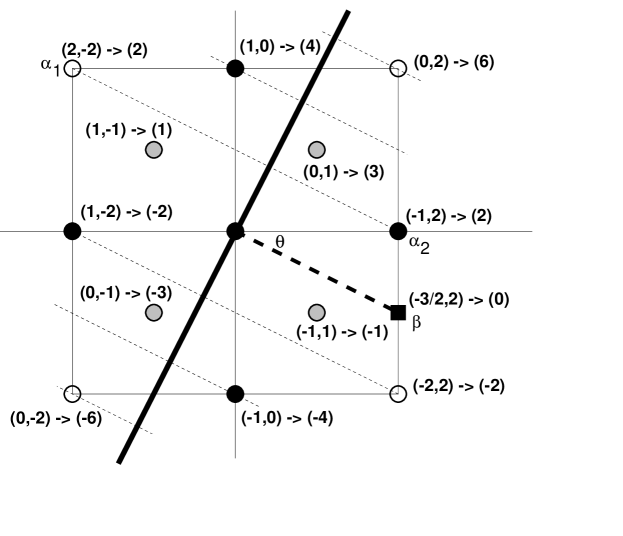
Figure 4: The irregular embedding of $SU(2)_{10}$ within $SO(5)_{1}$. The non-zero roots of $SO(5)_{1}$ lie along the outer square, with the empty circles denoting the long roots and the black circles denoting the short roots. The simple roots are $\vec{\alpha}_{1}$ and $\vec{\alpha}_{2}$. The non-zero weights of the 5 representation of $SO(5)$ comprise the short roots alone, and the weights of the 4 representation are also superimposed (shaded circles). Next to each weight we have listed its Dynkin labels, along with the Dynkin label of the $SU(2)$ weight to which it corresponds according to the embedding matrix in Eq. (5.7). The axis of $SU(2)$ projection is also shown (dark line), with the vector $\vec{\beta}$ (black square) chosen perpendicular to this axis. The Dynkin labels of $\vec{\beta}$ thus uniquely define this axis, and specify the orientation angle to be $\theta=\cos^{-1}(2/\sqrt{5})$.

Finally, it is also straightforward to determine the GSO projection that corresponds to this $SU(2)_{10}\subset SO(5)$ embedding. Using the formalism discussed in the previous section, we know that this $SO(5)$ group can be realized directly in a two-dimensional lattice, and indeed we find that these two lattice dimensions correspond to the orthogonal Cartesian axes indicated in Fig. 4, with $U_{1}$ and $U_{2}$ corresponding to the vertical and horizontal directions respectively. The nullspace vector $\vec{\beta}$, with Dynkin indices $(-3/2,2)$, then has Cartesian coordinates $(-1/2,1)$. Hence, in order to realize this embedding, we find that we must project out the linear combination of Cartan generators

$$SU(2)_{10}\subset SO(5)_{1}:~{}~{}~{}~{}~{}~{}{\rm project~{}out}~{}~{}~{}U_{1}-2\,U_{2}~{}=~{}\sqrt{5}\,\biggl{[}(\sin\,\theta)\,U_{1}-(\cos\,\theta)\,U_{2}\biggr{]}~{}.$$ (5.9)

Of course, in string theory, this original $SO(5)$ group factor must itself be realized from a level-one simply laced group via a prior dimensional truncation.

6 Satisfying the “Adjoint to Adjoint Only” Rule: A Pedagogical Example

In this section we shall take a brief detour, and discuss how the required sorts of dimensional truncations are actually realized in a particular string construction — one based upon real fermions [18, 16]. We shall assume no prior familiarity with this construction, and keep our presentation as non-technical as possible. However, by studying this example, we shall also be able to discuss how string theory manages to satisfy what we shall call the “adjoint to adjoint only” rule. As we have seen, a dimensional truncation is consistent if and only if it corresponds to a bona-fide irregular embedding. However, this is only part of the story. In particular, in the physical context of string theory, there is an additional constraint that comes into play.

6.1 The “adjoint to adjoint only” rule

In order to discuss this additional constraint, let us begin by recalling that under an irregular embedding of $G^{\prime}$ into $G$, the adjoint representation of $G$ generally decomposes into a sum of irreducible representations of $G^{\prime}$, one of which includes the adjoint of $G^{\prime}$:

$${\bf R}_{\rm adj}~{}\to~{}{\bf R^{\prime}}_{\rm adj}~{}+~{}{\rm other}~{}G^{\prime}~{}{\rm representations}~{}.$$ (6.1)

This causes no inconsistency as far as the mathematical embedding of the $G^{\prime}$ subgroup is concerned. However, within the physical context of string theory, a decomposition of the form (6.1) leads to serious problems. To see this, let us imagine the particular string model before introducing the final GSO projections that induce the dimensional truncation and break $G$ to $G^{\prime}$. In this parent string model, all of the gauge-boson states that fill out the adjoint representation of $G$ will be massless, and carry a spacetime vector index. However, according to (6.1), after the final GSO projections are performed, the states that survive will in general fill out not only the adjoint representation of $G^{\prime}$, but also “other” non-adjoint representations as well. However, all of these states will continue to be massless, and moreover they will all continue to carry a spacetime vector index. Thus, a priori, all of these states will give rise to gauge bosons. This is impossible, however, since such states will not fill out the adjoint of any Lie group! In other words, within the physical context of string theory, such a decomposition (6.1) would still not be consistent.

In general, string theory manages to avoid this problem in a very elegant fashion: the very same GSO projections that effect the dimensional truncation in the first place also simultaneously project the “other” unwanted $G^{\prime}$ representations out of the spectrum. In other words, string theory manages to enforce an “adjoint to adjoint only” rule. Clearly, this property goes beyond mere group theory, and is ultimately guaranteed by the self-consistency of the underlying string construction. It is therefore instructive to see how this arises in practice.

6.2 The “adjoint to adjoint only” rule: An example

The pedagogical example we shall consider demonstrates not only how the required sorts of GSO projections can be achieved in a particular string construction, but also how the “adjoint to adjoint only” rule is simultaneously and automatically enforced.

The example we shall consider consists of a simple worldsheet theory containing ten Majorana-Weyl fermions. In an actual string model, these two-dimensional fermions (which we shall label $\lambda_{1,...,10}$) might be part of the internal worldsheet degrees of freedom. Now, if these fermions are treated symmetrically (meaning that their excitations are all interchangeable and commute with the GSO projections in each sector), then the internal symmetry corresponding to these ten fermions is $SO(10)$. Typically the GSO constraints for such gauge boson states take the form

$$\sum_{i=1}^{10}N_{i}~{}=~{}2$$ (6.2)

where the real-fermion number operators $N_{i}$ are $1$ if the lowest mode of the $i^{\rm th}$ fermion is excited, and $0$ otherwise. This gives rise to $45$ different states, which comprise the adjoint of $SO(10)$. That this group is realized at level one is easily determined by calculating the central charge of this fermionic representation, $c_{\rm tot}=10\times 1/2=5$, and comparing with (2.6).

It is also possible to obtain these results by considering the charge lattice corresponding to the gauge bosons. This is done as follows. Because these ten real fermions are treated completely symmetrically by the single GSO constraint equation (6.2), it is possible to pair these fermions to form five complex fermions via $\psi_{k}\equiv(\lambda_{2k-1}+i\lambda_{2k})/\sqrt{2}$ for $k=1,...,5$. Through this relation, we can directly relate the particle and anti-particle excitation mode operators $b^{(a)}_{r},\overline{b}^{(a)}_{r}$ of the complex fermions $\psi_{a}$ to the particle excitation mode operators $d^{(i)}_{r}$ of the real fermions $\lambda_{i}$:

$$b^{(k)}_{r} = {1\over\sqrt{2}}\,\left(d_{r}^{(2k-1)}+i\,\overline{d}_{r}^{(2k)}\right)$$

$$\overline{b}^{(k)}_{r} = {1\over\sqrt{2}}\,\left(d_{r}^{(2k-1)}-i\,\overline{d}_{r}^{(2k)}\right)~{}.$$ (6.3)

Here the index $r$ signifies the energy of the excitation, odd half-integer for the Neveu-Schwarz sector (such as we encounter in this toy model, with the lowest mode $r=1/2$ producing the gauge bosons), and integer otherwise. Likewise, we can define the number operators for the individual real fermions, $N^{(i)}\equiv\sum_{r}\,d_{r}^{\dagger(i)}d_{r}^{(i)}$, as well as the complex-fermion number operators ${\cal N}_{a}$ for each complex fermion $\psi_{a}$: ${\cal N}^{(a)}\equiv\sum_{r}\,(b_{r}^{\dagger(i)}b_{r}^{(i)}-\overline{b}_{r}^{\dagger(i)}\overline{b}_{r}^{(i)})$. Thus ${\cal N}^{(a)}$ yields $+1$ for a single particle excitation, $-1$ for a single anti-particle excitation, and $0$ if both or neither are excited. Note that excitations of both of the real fermions $(\lambda_{2i-1},\lambda_{2i})$ in a single pair amount to a joint particle/anti-particle excitation in the corresponding complex fermion $\psi_{i}$. Hence, of the 45 gauge boson states above, five give rise to states with all ${\cal N}_{a}=0$, while the remaining 40 states have different configurations of non-zero $\vec{\cal N}$. Now, in the conventional normalization, the five-dimensional charge lattice ${\bf Q}$ corresponding to these gauge-boson states is simply the set of allowed $\vec{\cal N}$. Thus the five states with $\vec{\cal N}=0$ correspond to the generators of the Cartan subalgebra, and the 40 remaining states fill out the five-dimensional root lattice of $SO(10)$. This much is of course simply the standard realization of $SO(10)_{1}$ in terms of five complex fermions.

Let us now consider what happens if, along with the single GSO constraint equation (6.2), we impose two additional constraint equations of the form

$$N_{1}+N_{2}+N_{3}+N_{4} \in 2\,\mathchoice{\hbox{\cmss Z\kern-3.99994ptZ}}{\hbox{\cmss Z\kern-3.99994ptZ}}{\lower 0.9pt\hbox{\cmsss Z\kern-2.79996ptZ}}{\lower 1.2pt\hbox{\cmsss Z\kern-2.79996ptZ}}$$

$$N_{1}+N_{2}+N_{3}+N_{5} \in 2\,\mathchoice{\hbox{\cmss Z\kern-3.99994ptZ}}{\hbox{\cmss Z\kern-3.99994ptZ}}{\lower 0.9pt\hbox{\cmsss Z\kern-2.79996ptZ}}{\lower 1.2pt\hbox{\cmsss Z\kern-2.79996ptZ}}~{}.$$ (6.4)

Such extra constraint equations can be realized, for example, in string models built out of so-called “necessarily real fermions” [16]. It is clear that this has a number of consequences, among them a decrease in the number of surviving states.

In this example, it is straightforward to determine the residual subgroup that survives. Considering the three constraint equations (6.2) and (6.4) simultaneously, we see that no states are allowed in which either $\lambda_{4}$ or $\lambda_{5}$ are excited. Indeed, our set of allowed excitations splits into two disjoint groups, the first consisting of any two excitations from the set $\{\lambda_{1,2,3}\}$ (thereby giving rise to three possible states), and the second consisting of any two excitations from the set $\{\lambda_{6,7,...,10}\}$ (giving rise to ten states). These correspond to the adjoint representations of $SU(2)$ and $SO(5)$ respectively. It is also trivial to verify, at least in this case, that the $SU(2)$ symmetry is in fact realized at level two, since this $SU(2)$ gauge factor is now essentially represented in terms of the three real fermions $\lambda_{1,2,3}$, with total central charge $c=3/2$.

In this simple example, it was straightforward to deduce that the level of the $SU(2)$ gauge factor was increased thanks to an obvious representation in terms of three real fermions, and a quick comparison of the central charges involved. However, the same results can be obtained by considering the effects on the original $SO(10)$ charge lattice induced by the additional constraints in (6.4). Recall that the first step in determining the charge lattice was to determine a pairing or complexification of the real fermions, for it is only in terms of such complex fermions that $U(1)$ charges can be defined. However, with the new constraints (6.4) adjoined, we now see that no consistent complexifications are possible for all ten real fermions. The maximal number of complex fermions that can be formed is three (i.e., $\psi_{1}$, $\psi_{4}$, and $\psi_{5}$), corresponding to the rank of the resulting gauge group. Hence, in our former five-dimensional charge-vector space, we see that two dimensions have simply been extinguished. This is of course nothing but a dimensional truncation of the charge lattice, now explicitly realized through the sets of GSO projections (6.2) and (6.4).

In order to analyze this remaining charge lattice, let us first consider the three states which form the adjoint representation of the $SU(2)$ gauge group factor. In the notation $|N_{1},N_{2},N_{3},...\rangle$, these three states are $|1\rangle\equiv|1,1,0,...\rangle$, $|2\rangle\equiv|1,0,1,...\rangle$, $|3\rangle\equiv|0,1,1,...\rangle$. Let us describe these states in terms of the full five-dimensional space corresponding to the five complex fermions $\psi_{1,...,5}$. The state $|1\rangle$, in the operator language of the complex fermions, is nothing but $\psi_{1}^{\dagger}\psi_{1}$. This is therefore the Cartan generator of the $SU(2)$ group. For the remaining states, we may, for convenience, switch to a new basis defined by $|2^{\prime}\rangle\equiv(|2\rangle+i|3\rangle)/\sqrt{2}$ and $|3^{\prime}\rangle\equiv(|2\rangle-i|3\rangle)/\sqrt{2}$. Using the mode relations (6.3), we then find that these new states can be expressed in terms of the number operators ${\cal N}_{a=1,2}$ corresponding to the complex fermions $\psi_{1}$ and $\psi_{2}$ as

$$|2^{\prime}\rangle = {1\over\sqrt{2}}\,\biggl{(}|{\cal N}_{1}=1,{\cal N}_{2}=1\rangle+|{\cal N}_{1}=1,{\cal N}_{2}=-1\rangle\biggr{)}$$

$$|3^{\prime}\rangle = {1\over\sqrt{2}}\,\biggl{(}|{\cal N}_{1}=-1,{\cal N}_{2}=1\rangle+|{\cal N}_{1}=-1,{\cal N}_{2}=-1\rangle\biggr{)}~{}.$$ (6.5)

This is the description that would be appropriate if there truly existed a full five-dimensional charge space. However, the second and third dimensions of this lattice have actually been truncated. Thus, concentrating on only the eigenvalue of ${\cal N}_{1}$ (or equivalently, applying the above Cartan generator $\psi_{1}^{\dagger}\psi_{1}$ to determine the quantum numbers of our non-zero roots), we find that the $|2^{\prime}\rangle$ state corresponds to the positive root at the point $+1$ in the remaining one-dimensional $SU(2)$ root lattice, and that the $|3^{\prime}\rangle$ state corresponds to the lattice site at $-1$. These three shortened roots at lattice sites $\{0,\pm 1\}$ comprise the root system of $SU(2)_{2}$.

It is also instructive to consider how the non-simply laced group $SO(5)$ is realized from the remaining ten gauge bosons in this example — i.e., those which are constructed via any two excitations from the fermion set $\{\lambda_{6,7,...,10}\}$. Since we can consistently form the two complex fermions $\psi_{4,5}$ from the four real fermions $\lambda_{7,8,9,10}$, the six excitations involving only $\lambda_{7,8,9,10}$ give rise to points in the charge lattice of lengths zero or $\sqrt{2}$, as expected. These correspond to the two zero roots and the four long roots in the $SO(5)$ root system. However, because the four states involving excitations of both $\lambda_{6}$ and one of the remaining fermions all have components in the truncated directions, they suffer dimensional projections and are reduced in length from $\sqrt{2}$ to $1$. Their projections onto the surviving directions then form the four short roots of $SO(5)$, thereby completing the root system of this non-simply laced algebra.

Thus, to summarize the dimensional truncations in this ten-fermion example, we see that imposing the constraint (6.2) alone yields the gauge group $SO(10)_{1}$, and then additionally imposing only the first of the constraints in (6.4) breaks this gauge group to $SO(4)_{1}\times SO(6)_{1}$. However, imposing the final constraint in (6.4) effects the dimensional truncation, removing two dimensions from the total charge lattice. One of these dimensions is removed from the $SO(4)=SU(2)\times SU(2)$ lattice, and produces $SU(2)$ at level two in the manner that we have already outlined in Fig. 2. The other dimension is removed from the $SO(6)=SU(4)$ lattice, and produces the non-simply laced group $SO(5)_{1}$.

Moreover, this ten-fermion example also shows precisely how the “adjoint to adjoint only” rule is automatically satisfied. In this example, the 15 representation of $SO(6)$ decomposes into the 10 and 5 representations of $SO(5)$. However, the third GSO constraint, which not only effects the dimensional truncation of the charge lattice, also projects out the 5 representation. Thus, only the adjoint 10 representation of $SO(5)$ survives. Similarly, of the original gauge bosons of $SO(4)=SU(2)\times SU(2)$, only one copy of the $SU(2)$ gauge bosons survives. Thus, as required, we see that the GSO projections that effect the dimensional truncation also simultaneously project out the non-adjoint representations, so that only the adjoint representation of the final subgroup survives.

7 Classification of String GUT Group Embeddings

As we have shown in Sects. 3 and 4, higher-level and/or non-simply laced gauge symmetries can arise in free-field heterotic string constructions only through dimensional truncations of the charge lattice, which correspond uniquely to irregular embeddings. Irregular embeddings, however, have been completely classified by mathematicians. Thus, by virtue of our identification, we now have at our disposal the means for a powerful classification of the possible embeddings through which such gauge symmetries can be realized in free-field string constructions. This will enable us to answer questions of direct relevance to string GUT model-builders, such as classifying all possible ways of realizing, e.g., $SU(5)_{2}$ or $SO(10)_{2}$ gauge groups in free-field string models.

In this section, we shall perform such a classification. We shall begin in Sect. 7.1 by recalling the reasons that higher-level GUT groups are of interest in string theory, and then we shall proceed in Sect. 7.2 to describe the mathematical classification of irregular embeddings. In Sect. 7.3 we will then use these results to completely classify all methods of obtaining $G_{\rm GUT}$ at levels $k=2,3,4$, for the cases $G_{\rm GUT}=SU(5)$, $SU(6)$, $SO(10)$, and $E_{6}$; furthermore, we shall prove in Sect. 7.3.5 that it is impossible to realize $SO(10)_{k>4}$ or $(E_{6})_{k>3}$ in free-field string theory. The material in Sects. 7.2 and 7.3 is fairly technical, and is not necessary for understanding the final results of our classification. We have therefore collected together and summarized the results of our GUT classification in Sect. 7.4, which can be read independently of the other sections.

7.1 Why higher-level GUT groups?

Affine Lie algebras with levels $k>1$ are of particular interest in string theory because their unitary representations include various phenomenologically desired representations which are otherwise precluded at levels $k=1$. These include, for example, the adjoint representations which are necessary for Higgs scalars in order to realize the standard symmetry-breaking scenarios of most conventional GUT theories, such as those of $SU(5)$ or $SO(10)$. In general, the unitary irreducible representations of a given affine Lie algebra at level $k$ (and consequently, the only representations that can appear in a consistent string model realizing such an algebra) are those for which

$$k~{}\in~{}\mathchoice{\hbox{\cmss Z\kern-3.99994ptZ}}{\hbox{\cmss Z\kern-3.99994ptZ}}{\lower 0.9pt\hbox{\cmsss Z\kern-2.79996ptZ}}{\lower 1.2pt\hbox{\cmsss Z\kern-2.79996ptZ}}~{}~{}~{}~{}~{}{\rm and}~{}~{}~{}~{}~{}~{}0~{}\leq~{}\sum_{i=1}^{{\rm rank}(G)}a_{i}\,m_{i}~{}\leq~{}k~{}$$ (7.1)

where $m_{i}$ are the so-called “co-marks” corresponding to each simple root $\vec{\alpha}_{i}$, and where $a_{i}$ are the Dynkin labels of the highest weight of the representation. The conformal dimension of such a representation is then given by

$$h_{(R)}~{}=~{}{C^{(R)}_{G}/\vec{\alpha}_{h}^{2}\over k+\tilde{h}_{G}}$$ (7.2)

where $C^{(R)}_{G}$ is the eigenvalue of the quadratic Casimir acting on the representation $R$. This eigenvalue is defined analogously to (2.3), via

$$\sum_{a=1}^{{\rm dim}(G)}\,(T^{a}T^{a})_{ij}~{}=~{}C^{(R)}_{G}\,\delta^{ij}$$ (7.3)

where $T^{a}$ are the group generators in the representation $R$. In general, $C^{(R)}_{G}=(\vec{\Lambda},\vec{\Lambda}+2\vec{\delta})$ where $\vec{\Lambda}$ and $2\vec{\delta}$ are respectively the highest root and the sum of the positive roots of $G$. Thus, the conformal dimension $h^{(R)}$ is directly related to the quadratic index $\ell_{G}(\vec{\Lambda})$ of the representation, as defined in (4.4), via

$$h_{(R)}~{}=~{}{{\rm dim}\,G\over{\rm dim}\,R}~{}{1\over k+\tilde{h}_{G}}~{}{\ell_{G}(\vec{\Lambda})\over\vec{\alpha}_{h}^{2}}~{}.$$ (7.4)

In heterotic string theory, a particular representation $R$ can appear in the massless spectrum if and only if its conformal dimension satisfies $h_{(R)}\leq 1$. This, along with the unitarity constraint (7.1), then limits the allowed representations that may appear for a given gauge group realized at a given affine level. Below, we have tabulated the complete set of unitary representations that can appear in the massless string spectrum for the phenomenologically interesting gauge groups $SU(5)$, $SU(6)$, $SO(10)$, and $E_{6}$ at levels $1\leq k\leq 4$. In each case, we have listed the values of $({\bf{dim(R)}},h_{(R)})$ for each such representation, and have also listed the central charge corresponding to the relevant group factor. Note that for each group $G_{k}$, the maximum affine level $k_{\rm max}$ that is a priori allowed is determined by requiring that $c(G_{k})\leq 22$.

$$SU(5)$$

() () () ()

 (5, 2/5) (10, 3/5)  (6, 5/12) (15, 2/3) (20, 3/4)  (10, 1/2) (16, 5/8)  (27, 2/3)

 (5, 12/35) (10, 18/35) (15, 4/5) (24, 5/7) (40, 33/35) (45, 32/35)  (6, 35/96) (15, 7/12) (20, 21/32) (21, 5/6) (35, 3/4) (84, 95/96)  (10, 9/20) (16, 9/16) (45, 4/5) (54, 1)  (27, 13/21) (78, 6/7)

 (5, 3/10) (10, 9/20) (15, 7/10) (24, 5/8) (40, 33/40) (45, 4/5) (75, 1)  (6, 35/108) (15, 14/27) (20, 7/12) (21, 20/27) (35, 2/3) (70, 11/12) (84, 95/108) (105, 26/27)  (10, 9/22) (16, 45/88) (45, 8/11) (54, 10/11) (120, 21/22) (144, 85/88)  (27, 26/45) (78, 4/5)

 (5, 4/15) (10, 2/5) (15, 28/45) (24, 5/9) (40, 11/15) (45, 32/45) (50, 14/15) (70, 14/15) (75, 8/9)  (6, 7/24) (15, 7/15) (20, 21/40) (21, 2/3) (35, 3/5) (70, 33/40) (84, 19/24) (105, 13/15) (120, 119/120) (189, 1)  (10, 3/8) (16, 15/32) (45, 2/3) (54, 5/6) (120, 7/8) (144, 85/96) (210, 1) cannot be realized in free-field string theory

(7.5)

Note that in the above table we have not listed singlet representations [for which the corresponding entry is (1,0) for all groups and levels]. We have also omitted the complex-conjugate representations, and representations obtained from those listed above via exchange of the simple roots when such exchanges are symmetries of the Dynkin diagram. In the cases of distinct representations having the same dimension [such as the 70 representations of $SU(5)$ and the 210 representations of $SO(10)$], we have adopted the primed labelling conventions of Ref. [21]. Furthermore, note that in our calculations of the conformal dimensions, we have assumed that each representation of a given group $G$ transforms as a singlet under all other group factors. Otherwise, for representations that are charged with respect to several groups simultaneously, one need only add the corresponding conformal dimensions.

There are several things to note from this table. First, note that $E_{6}$ at affine levels $k\geq 4$ cannot be realized in free-field string models. Although the central charge of such a group factor at $k=4$ would only be $39/2$ — which is less than 22 and hence potentially realizable — we will prove later in this section (as the result of our classification) that there are ultimately no string-theoretic embeddings for $E_{6}$ at such levels $k\geq 4$. We thereby conclude that the only massless representations of $E_{6}$ that can ever be realized in free-field string models are the ${\bf{27}}$ and ${\bf{78}}$ representations.

Second, note that the ${\bf{126}}$ representation of $SO(10)$ does not appear for $SO(10)$ realizations at levels $1\leq k\leq 4$. Indeed, the first level for which the ${\bf{126}}$ can potentially appear in the massless string spectrum is $k_{SO(10)}=5$. Like the $E_{6}$ case, however, we will prove later in this section (again as a result of our classification) that the maximum affine level at which $SO(10)$ can ever be realized is in fact $k=4$. Thus, it is impossible to realize the ${\bf{126}}$ representation of $SO(10)$ in free-field heterotic string theory. This result is completely general, and applies for all free-field string constructions.

Most importantly, however, we see from this table that regardless of the GUT gauge group in question, we cannot achieve the desired massless adjoint representation required for the GUT Higgs scalar unless the GUT group is realized at an affine level $k\geq 2$. Moreover, in order to avoid too many unwanted representations appearing in the massless string spectrum, one usually wishes to keep the affine level from being too large. Typically, the choices $2\leq k\leq 4$ are of direct phenomenological interest, especially for the standard GUT groups such as $SU(5)$, $SU(6)$, $SO(10)$, and $E_{6}$.

We therefore seek to classify the ways in which such groups and levels can be realized in free-field string constructions.

7.2 Classification of irregular embeddings

We begin by listing the mathematical results for the complete classification of irregular embeddings. As far as we are aware, the results of a complete classification do not appear in any one place in the mathematics or physics literature. We have therefore gleaned and compiled the following classification from various different sources [24, 21], most notably the original papers of Dynkin [22, 25].

It turns out that there are only three classes of embeddings that we need to consider, each with its own set of rules. These three classes correspond to the following irregular embeddings: embeddings of simple algebras into classical algebras (which we shall call Class I), embeddings of non-simple algebras into classical algebras (Class II), and embeddings of all algebras into exceptional algebras (Class III). Note that, as in previous sections, we use a notation in which $SU(r+1)$, $SO(2r)$, $Sp(2r)$, and $SO(2r+1)$ each have rank $r$.

Class I: Of the three classes we shall consider, the irregular embeddings of simple algebras into classical algebras are the most complicated. Nevertheless, the general property that governs such embeddings is most easily stated as follows. For each simple group $G^{\prime}$ and for each $n$-dimensional irreducible representation ${\bf{n}}$ of $G^{\prime}$, there always exists at least one irregular embedding of $G^{\prime}$ into a larger-rank classical group $G^{\prime\prime}$ which also has an $n$-dimensional irreducible representation. In each case, such $G^{\prime}\subset G^{\prime\prime}$ embeddings then give rise to the branching rule ${\bf{n}}\to{\bf{n}}$. If $G$ is the smallest of such groups $G^{\prime\prime}$ (so that there exists no proper subgroup of $G$ which contains $G^{\prime}$), then the embedding $G^{\prime}\subset G$ is called maximal. In order to achieve a classification of embeddings, one therefore focuses on maximal embeddings, since these can be iterated in order to reproduce all other embeddings.

The sets of maximal embeddings $G^{\prime}\subset G$ generally come in two distinct patterns, which we shall label Class IA and Class IB. Class IA maximal embeddings are those that arise from the following “theorem”: for almost every $n$-dimensional representation ${\bf{n}}$ of $G^{\prime}$, the following is a maximal irregular embedding:

$${\rm if~{}{\bf{n}}~{}is~{}real}~{} ~{}~{}\Longrightarrow ~{}~{}~{}G^{\prime}_{k^{\prime}}\subset SO(n)_{2}$$

$${\rm if~{}{\bf{n}}~{}is~{}pseudo{-}real}~{} ~{}~{}\Longrightarrow ~{}~{}~{}G^{\prime}_{k^{\prime}}\subset Sp(n)_{1}$$

$${\rm if~{}{\bf{n}}~{}is~{}complex}~{} ~{}~{}\Longrightarrow ~{}~{}~{}G^{\prime}_{k^{\prime}}\subset SU(n)_{1}~{}.$$ (7.6)

In (7.6), the subscripts indicate the affine levels of the embeddings, with $k^{\prime}$ in each case given by $k^{\prime}=\ell_{G^{\prime}}({\bf{n}})$ where $\ell_{G^{\prime}}({\bf{n}})$ is the index (4.4) of the ${\bf{n}}$ representation of $G^{\prime}$. These affine levels have been determined as follows. Thanks to the simple branching rules ${\bf{n}}\to{\bf{n}}$ that arise in such embeddings, we see that we can easily determine the affine level of the irregular $G^{\prime}$ subgroup in each case by comparing, as in (4.6), the index of the ${\bf{n}}$ representation of $G^{\prime}$ with the index of the fundamental representation of the group in which it is embedded according to (7.6). In general, the index of the fundamental representation for these latter groups (in our present normalization with longest roots of length $\sqrt{2}$ for all groups) is

$$\ell_{SU(n)}\,({\rm fundamental}) = 1~{}$$

$$\ell_{SO(2n+1)}\,({\rm fundamental}) = 2~{}$$

$$\ell_{Sp(2n)}\,({\rm fundamental}) = 1~{}$$

$$\ell_{SO(2n)}\,({\rm fundamental}) = 2~{}.$$ (7.7)

Thus, the level of the $G^{\prime}$ subgroup in each case becomes simply the index $\ell_{G^{\prime}}({\bf{n}})$ of the ${\bf{n}}$ representation of $G^{\prime}$. Of course, for consistency, these indices must be calculated in a normalization for which the longest roots of $G^{\prime}$ have length $\sqrt{2}$.

As an example of the rule (7.6), let us consider the irregular embeddings of $SU(3)$. Recall that the representations of $SU(3)$ can be labelled by the two Dynkin indices $(a_{1},a_{2})$ of their highest weights; the corresponding representation is then real if $a_{1}=a_{2}$, and complex otherwise. Thus, by scanning the irreducible representations of $SU(3)$, we easily find that $G^{\prime}\equiv SU(3)$ can be maximally irregularly embedded in all of the following groups at level one: $SU(3)$ (with $k_{G^{\prime}}=1$), $SU(6)$ (with $k_{G^{\prime}}=5$), $SO(8)$ (with $k_{G^{\prime}}=3$), $SU(10)$ (with $k_{G^{\prime}}=15$), $SU(21)$ (with $k_{G^{\prime}}=70$), and so forth. (The group $SU(15)$ is omitted for reasons to be explained.) Of course, the first of these embeddings is that of $SU(3)$ into itself, and does not correspond to a change in the affine level.

Unfortunately, there are several special cases in which the embeddings (7.6), though valid, are not maximal. An example of such a special case is the ${\bf{15}}$ representation of $SU(3)$: the above rule would assert that the embedding into $G=SU(15)$ is maximal, whereas in fact the true maximal embedding satisfying the ${\bf{15}}\to{\bf{15}}$ branching rule is the same one that also simultaneously satisfies the ${\bf{6}}\to{\bf{6}}$ branching rule, namely $SU(3)_{5}\subset SU(6)_{1}$. The complete set of special cases of (7.6) has been enumerated by Dynkin, but for the purposes of analyzing embeddings involving the string GUT groups, we shall require only those special cases for which $G^{\prime}$ has rank $\geq 5$ and $G$ has rank $\leq 22$. The complete set of such special cases is then the following:

$$\vec{\Lambda}^{\prime}$$

,

, ,

, , , odd

;

(7.8)

For each case listed in (7.8), we have indicated the relevant representation(s) of $G^{\prime}$ by specifying the non-zero Dynkin labels of its highest weight(s) $\vec{\Lambda}^{\prime}$ in $G^{\prime}$. Thus, except for the special cases (7.8), the complete set of Class IA maximal irregular embeddings is given by (7.6). We have calculated the affine levels in (7.8) following the procedure discussed above.

The maximal irregular embeddings in Class IB follow a different set of embedding patterns. Those for which $G^{\prime}$ has rank $\geq 4$ and $G$ has rank $\leq 22$, along with some of the relevant representation(s) satisfying the ${\bf{n}}\to{\bf{n}}$ branching rule in each case, are as follows:

$${\bf{n}}: ~{}~{}SO(n)_{2}~{} \subset~{}SU(n)_{1}$$

$${\bf{n}}: ~{}~{}Sp(n)_{1}~{} \subset~{}SU(n)_{1}$$

$$a_{n}=k,~{}k\geq 2: ~{}~{}SO(2n+1)_{1}~{} \subset~{}SO(2n+2)_{1}~{}.$$ (7.9)

Note that the third special case in (7.8) therefore reproduces a pattern in Class IB rather than a pattern in Class IA. As before, we have determined the affine levels in (7.9) via (7.7). Note that the last two embeddings in (7.9) give rise to subgroups which are not at higher levels, but which instead are non-simply laced.

Class II: Irregular embeddings of non-simple algebras into classical algebras also fall into simple patterns which can be grouped into two subclasses. For Class IIA, a complete list of rules is the following:

$$SU(m)_{n}~{}\times~{}SU(n)_{m}~{} \subset ~{}SU(mn)_{1}$$

$$SO(m)_{n}~{}\times~{}SO(n)_{m}~{} \subset ~{}SO(mn)_{1}$$

$$SO(m)_{2n}~{}\times~{}Sp(n)_{m}~{} \subset ~{}Sp(mn)_{1}$$

$$Sp(m)_{n/2}~{}\times~{}Sp(n)_{m/2}~{} \subset ~{}SO(mn)_{1}~{}.$$ (7.10)

Once again, these embeddings are maximal, and have a simple branching rule relating their respective fundamental representations: ${\bf{mn}}\to({\bf{m}},{\bf{n}})$. It is this branching rule which has allowed us to determine the affine levels listed in (7.10). To see this, let us consider the first embedding in (7.10), namely $SU(m)\times SU(n)\subset SU(mn)$, and let us assume that the $SU(mn)$ factor is realized at level one. Then, since the branching rule for the fundamental representations is ${\bf{mn}}\to({\bf{m}},{\bf{n}})$, we see that as far as the $SU(m)$ subgroup factor is concerned, this branching rule essentially amounts to ${\bf{mn}}\to{\bf{m}}+{\bf{m}}+...~{}{\bf{m}}$ (where the ${\bf{m}}$ representation appears $n$ times). Thus, given (7.7), we see that the affine level of the $SU(m)$ factor is simply $k_{SU(m)}=n$, and likewise $k_{SU(n)}=m$. All of the affine levels given in (7.10) are determined in this way. Note, in particular, that the results for the last embedding listed in (7.10) are consistent since $n/2$ and $m/2$ are necessarily integers.

As examples of the Class IIA embeddings, let us once again consider potential realizations of $SU(3)$ at higher levels. In addition to those found above (which follow from the Class IA embeddings), we now have the embeddings $SU(3)_{n}\subset SU(3n)$ for all $n\geq 1$. These follow from the Class IIA embedding pattern

$$SU(3)_{n}\times SU(n)_{3}~{}\subset~{}SU(3n)_{1}~{}.$$ (7.11)

As explained in the Appendix, however, these embeddings ultimately turn out to be equivalent to the diagonal embeddings

$$SU(3)_{n}~{}\subset~{}SU(3)_{1}\times SU(3)_{1}\times SU(3)_{1}\times....~{}\subset~{}SU(3n)_{1}~{}.$$ (7.12)

Thus, we do not obtain new non-diagonal embeddings in this case.

Indeed, as we shall discuss in the Appendix, it turns out to be a general property that all of the embeddings in (7.10) are ultimately equivalent to diagonal embeddings once they are “turned around” and expressed as a simple group embedded in a non-simple group. This includes not only the $SU(n)$ embeddings, as discussed above, but also the $SO(n)$ and $Sp(n)$ embeddings. We conclude, therefore, that the Class IIA embeddings are all equivalent to the diagonal embedding of any level-$n$ group $G$ within an $n$-fold tensor product of level-one factors of $G$:

$$G_{n}~{}\subset~{}G_{1}\times G_{1}\times...\times G_{1}~{}=~{}\mathop{\bigotimes}_{i=1}^{n}\,G^{(i)}_{1}~{}.$$ (7.13)

Of course, as we know, this diagonal embedding pattern extends even to the cases when $G$ is one of the exceptional groups.

In this context, it is worth observing that the existence of such diagonal embeddings (7.13) in turn implies the existence of more general embeddings of the form

$$G_{K}~{}\subset~{}\mathop{\bigotimes}_{i=1}^{n}\,G_{k_{i}}^{(i)}~{}~{}~{}~{}{\rm where}~{}K\equiv\sum_{i=1}^{n}k_{i}~{}$$ (7.14)

for all groups $G$. This embedding is more subtle than it may at first appear, for while it is clear from (7.13) that

$$\mathop{\bigotimes}_{i=1}^{n}\,G_{k_{i}}^{(i)}~{}\subset~{}\mathop{\bigotimes}_{i=1}^{K}\,G_{1}^{(i)}~{}~{}~{}~{}~{}{\rm where}~{}K\equiv\sum_{i=1}^{n}k_{i}~{},$$ (7.15)

it is not obvious that the relation (7.14) actually follows as a result. In other words, while both $G_{K}$ and $\otimes_{i}G_{k_{i}}^{(i)}$ are subgroups of $G_{1}\times G_{1}\times...\times G_{1}$, it is not clear that these subgroups are actually related to each other as in (7.14). However, it turns out that (7.14) is indeed valid. This is most easily demonstrated via the dimensional truncation procedure described in Sect. 3, in particular via a generalization of Fig. 2 to the case when two identical group factors $G_{k_{1}}\times G_{k_{2}}$ are realized at different levels. In such cases, the axis of truncation does not have an orientation angle $\theta=45^{\circ}$ as in Fig. 2, but rather an orientation angle $\theta=\tan^{-1}(k_{2}/k_{1})$. Induction then demonstrates (7.14) for all $n$.

We now turn to the Class IIB embeddings. These embeddings consist of the single general rule

$$SO(s)_{1}~{}\times~{}SO(t)_{1}~{}\subset~{}SO(s+t)_{1}~{}~{}~{}~{}{\rm for}~{}s,t~{}{\rm odd}~{},$$ (7.16)

with the branching rule for the fundamental representation given by $({\bf{s+t}})\to({\bf{s}},{\bf 1})+({\bf 1},{\bf{t}})$. Once again, we have determined the affine levels in (7.16) via this branching rule and (4.6). For the $SO(s)$ group factor, the relevant branching rule is essentially $({\bf{s+t}})\to{\bf{s}}+{\bf 1}+{\bf 1}+...+{\bf 1}$ where there are a total of $t$ singlets (each of which has vanishing index). Thus, we find that $k_{SO(s)}=1$, and likewise $k_{SO(t)}=1$. Note that like the last two Class IB embeddings, these Class IIB embeddings also give rise to subgroups which are non-simply laced rather than at higher levels.

Class III: Finally, we consider the case of irregular embeddings into the exceptional groups. In this case, there does not exist a general rule. Nevertheless, all such embeddings have been compiled, yielding the following complete list:

$$SU(2)_{28}~{} \subset ~{}(G_{2})_{1}$$

$$SU(2)_{156},\,SU(2)_{8}\times(G_{2})_{1}~{} \subset ~{}(F_{4})_{1}$$

$$SU(3)_{9},\,Sp(8)_{1},\,(F_{4})_{1},\,(G_{2})_{3},\,SU(3)_{2}\times(G_{2})_{1}~{} \subset ~{}(E_{6})_{1}$$

$$SU(2)_{231},\,SU(2)_{399},\,SU(3)_{21},\,SU(2)_{15}\times SU(2)_{24},~{}~{}~{}~{}$$

$$SU(2)_{7}\times(G_{2})_{2},\,SU(2)_{3}\times(F_{4})_{1},\,Sp(6)_{1}\times(G_{2})_{1}~{} \subset ~{}(E_{7})_{1}$$

$$SU(2)_{520},\,SU(2)_{760},\,SU(2)_{1240},\,SO(5)_{12},~{}~{}~{}~{}$$

$$SU(2)_{16}\times SU(3)_{6},\,(F_{4})_{1}\times(G_{2})_{1}~{} \subset ~{}(E_{8})_{1}~{}.$$ (7.17)

In writing this list of Class III embeddings, we have explicitly included the affine levels of the subgroups, as originally calculated by Dynkin. These affine levels are calculated directly from (4.6). All of these embeddings are maximal.

7.3 Realizing the GUT groups $SU(5)$, $SU(6)$, $SO(10)$, and $E_{6}$ at higher levels

Given the above results, we now seek to classify the methods by which phenomenologically interesting GUT groups such as $G_{\rm GUT}=SU(5)$, $SU(6)$, $SO(10)$, and $E_{6}$ can be realized at higher levels, e.g., $k=2,3,...$. As we have already seen, such higher-level realizations of these groups are typically obtained in the literature as the diagonal component within a tensor product of multiple copies of the level-one group. Such diagonal embeddings, however, tend to make it difficult (though not impossible) to simultaneously obtain three generations. We therefore seek to know whether there might exist other potentially useful embeddings which are also capable of yielding $(G_{\rm GUT})_{k}$ for, e.g., $k=2$, $k=3$, and $k=4$. In this section, we shall give a complete classification of all embeddings that realize these groups at levels $k=2$, $k=3$, and $k=4$. In the case of $SO(10)$, we will actually extend this classification to $k=7$ (which is the maximum level allowed by central-charge constraints). Of course, the methods that we shall use are applicable to all groups and levels.

7.3.1 Classifying GUT Embeddings: “initially irregular” vs. “initially regular”

Recall that free-field string constructions require that a higher-level gauge group ultimately be realized as a subgroup of a level-one simply laced group (henceforth denoted “L1SL”) of rank $\leq 22$. In general, there are various ways in which this can be done, through sequences of both regular and irregular embeddings involving an entire chain of intermediate groups $G_{i}$. It is therefore first necessary to find an efficient way of organizing our classification procedure.

In our case, we are interested in specifying a particular smallest subgroup (e.g., $SU(5)$ or $SO(10)$ at a particular affine level). We are less interested in specifying the large group into which these subgroups are embedded, provided it is an L1SL of appropriate rank. (Indeed, building our embeddings from the ground up, we see that once we obtain an L1SL of appropriate rank, we can always append purely regular embeddings in order to embed this group into the expected $SO(44)$ gauge group or into any of its enhanced L1SL’s such as $E_{8}\times E_{8}\times...$.) Therefore, for the purposes of our investigation, the primary distinction that naturally arises will involve the sorts of smallest or initial embeddings that we shall use.

To this end, we shall first invent some terminology. “Initially irregular embeddings” will correspond to embeddings in which the $SU(5)_{k}$ or $SO(10)_{k}$ subgroup factor is realized directly as the result of a maximal irregular embedding into some intermediate group $G^{\ast}$. In other words, the first embedding in the sequence of maximal embeddings $G_{\rm GUT}\subset G^{\ast}\subset...\subset$ L1SL must be irregular. In some cases, this group $G^{\ast}$ will be an L1SL itself, in which case we are done. Otherwise, if the group $G^{\ast}$ is non-L1SL, we then iterate the procedure. Note that in this subsequent iteration that embeds $G^{\ast}$ into an L1SL, we do not limit ourselves to only sequences of maximal irregular embeddings; regular embeddings are also permitted. Of course, in order to change the non-L1SL group $G^{\ast}$ into an L1SL, at least one irregular embedding must appear in this subsequent iteration. Nevertheless, we refer to such combined embeddings of $G_{\rm GUT}\subset$ L1SL as “initially irregular” because the lowest initial embedding is irregular.

The remaining possible route for achieving higher-level GUT groups will therefore involve the “initially regular embeddings”. Such initially regular embeddings first realize $(G_{\rm GUT})_{k}$ as a regular subgroup of the first intermediate group $G^{\ast}$. Note that we do not require that this initial regular embedding of $G_{\rm GUT}$ into $G^{\ast}$ be maximal, since sequences of maximal regular embeddings are also regular. Thus, in general $G^{\ast}$ is defined as the highest group $G_{i}$ in the sequence $G_{\rm GUT}\subset G_{1}\subset G_{2}\subset...\subset$ L1SL that can be reached from $G_{\rm GUT}$ through only regular embeddings. We then subsequently seek to realize $G^{\ast}$ via an embedding (necessarily irregular, but not necessarily maximal) into an L1SL. Note that this subsequent embedding of $G^{\ast}\subset$ L1SL is itself initially irregular.

These “initially regular” embeddings of $(G_{\rm GUT})_{k}$ into an L1SL generally proceed through two types of intermediate group $G^{\ast}$. The first type is a level-$k$ simply or non-simply laced group; in such cases the regular embedding of $SU(5)_{k}$ or $SO(10)_{k}$ into $G^{\ast}$ is constructed using only the long roots of $G^{\ast}$. We shall call these “long-root embeddings”. If $k\in 2\mathchoice{\hbox{\cmss Z\kern-3.99994ptZ}}{\hbox{\cmss Z\kern-3.99994ptZ}}{\lower 0.9pt\hbox{\cmsss Z\kern-2.79996ptZ}}{\lower 1.2pt\hbox{\cmsss Z\kern-2.79996ptZ}}$, then a second possible type of intermediate group $G^{\ast}$ is a level-$(k/2)$ non-simply laced intermediate group $G^{\ast}$; in such cases, $(G_{\rm GUT})_{k}$ is realized through regular embeddings constructed from the short roots of $G^{\ast}$. We shall call these “short-root embeddings”. We have already seen examples of such short-root regular embeddings in (4.1).

Thus, in order to realize a particular higher-level gauge group, we must consider both “initially irregular” embeddings, and long- and short-root “initially regular” embeddings. These classifications exhaust all possibilities. We shall therefore examine each case in turn.

7.3.2 Initially irregular embeddings of the GUT groups

We begin by studying the initially irregular embeddings of $SU(5)_{k}$, $SU(6)_{k}$, and $SO(10)_{k}$ into an L1SL. We shall first focus on the cases in which such embeddings are maximal, and then proceed to the non-maximal cases.

Maximal embeddings:   We begin with the possibilities provided by the maximal Class IA embeddings listed in (7.6). In general, the representations of $SU(5)$ can be described by the four Dynkin indices $(a_{1},a_{2},a_{3},a_{4})$ of their highest weights; the representation is real if $a_{1}=a_{4}$ and $a_{2}=a_{3}$, and complex otherwise. Thus, we find that there exist non-trivial irregular embeddings of $SU(5)$ into only the following groups with rank $\leq 22$: $SU(10)$, $SU(15)$, and $SO(24)$. Calculating the affine levels of the $SU(5)$ subgroup in each case, however, we find that only the embedding into $SU(10)$ realizes $SU(5)$ with an affine level less than or equal to four: $SU(5)_{3}\subset SU(10)_{1}$. (The $SU(5)$ levels in the other two cases are seven and five respectively.) Thus, only the $SU(5)_{3}\subset SU(10)_{1}$ embedding is suitable for the purposes of our classification. This is indeed an efficient way of realizing $SU(5)_{3}$, for it requires only the rank-nine group $SU(10)_{1}$ rather than the rank-12 group $[SU(5)_{1}]^{3}$ that would have been required for the straightforward diagonal embedding.

Likewise, for the $SU(6)$ GUT group, we find that only the embedding $SU(6)_{4}\subset SU(15)_{1}$ satisfies our criteria of having $k_{\rm GUT}\leq 4$ and rank $G\leq 22$.

In the case of the $SO(10)$ GUT group, recall that the representations of $SO(10)$ are described by five Dynkin labels $(a_{1},a_{2},a_{3},a_{4},a_{5})$, with an ordering for which $a_{4}$ and $a_{5}$ correspond to the spinor labels. In general, these representations are real if $a_{4}=a_{5}$, and complex otherwise. Hence, we find that (7.6) yields only one non-trivial embedding possibility into a group of rank and central charge less than 22, namely $SO(10)\subset SU(16)$. Comparing the indices of these representations, we then find that the level of the $SO(10)$ factor in this embedding is $k=4$. Thus $SO(10)_{4}\subset SU(16)_{1}$. Note that such an embedding is particularly useful if we wish to realize $SO(10)_{4}$, especially since the diagonal method would have required the rank-20 group $[SO(10)_{1}]^{4}$.

This concludes the possibilities that arise from Class IA embeddings. We now examine the possible embeddings from the other classes. A priori, it is possible that some of the Class IA special cases listed in (7.8) can yield embeddings for our GUT groups $G_{\rm GUT}$ at at affine levels $2\leq k\leq 4$. The special cases involving $SU(5)$ pertain to its ${\bf{45}}$ and ${\bf{105}}$ representations; likewise, the special cases involving $SU(6)$ pertain to its ${\bf{105}}$ and ${\bf{210}}$ representations, and the special case involving $SO(10)$ pertains to its ${\bf{560}}$ representation. Comparing the indices of these representations, however, we find that these special cases merely reproduce the above Class IA embeddings. Thus, we do not obtain any new embeddings from the Class IA special cases.

Turning to Class IB embeddings, however, we see that while no new Class IB possibility exists for realizing $SU(5)_{k}$ or $SU(6)_{k}$ with $k>1$, we now have the single new possible Class IB embedding for $SO(10)_{2}$: $SO(10)_{2}\subset SU(10)_{1}$.

Finally, as we have already discussed, the Class IIA embeddings are equivalent to the diagonal embeddings, and the Class IIB embeddings do not embed any of our GUT groups of interest. Likewise, scanning the Class III embeddings, we see that in no case are the subgroups of sufficient rank to be of interest to us.

We thus conclude that the following is the complete list of maximal initially irregular embeddings which are of interest to us:

$$\#1: ~{}~{}~{}~{}SU(5)_{3}~{} \subset~{}SU(10)_{1}$$

$$\#2: ~{}~{}~{}~{}SU(6)_{4}~{} \subset~{}SU(15)_{1}$$

$$\#3: ~{}~{}~{}~{}SO(10)_{2}~{} \subset~{}SU(10)_{1}$$

$$\#4: ~{}~{}~{}~{}SO(10)_{4}~{} \subset~{}SU(16)_{1}~{}.$$ (7.18)

Note that we do not list the corresponding diagonal embeddings, which in principle are also possible. We have numbered the embeddings in (7.18) for future ease of reference.

Non-maximal embeddings:   We now consider the non-maximal initially irregular embeddings. Note that if we are to embed $SU(5)_{k}$, $SU(6)_{k}$, or $SO(10)_{k}$ via a non-maximal initially irregular embedding into an L1SL, then for the $k=2$ and $k=3$ cases, the initial maximal irregular embedding in the series must embed the GUT group into a group $G^{\ast}$ which is necessarily non-simply laced, and realized either at level $k$ or at level one. This is because any embedding into a simply laced group at level $k$ would be a regular embedding (which will be considered later, as an “initially regular” embedding); likewise, any such embedding into a simply laced group at level one would have already been sufficient for our purposes, and would therefore have already been classified above as a maximal “initially irregular” embedding. A quick examination of the possible maximal irregular embeddings then shows that there do not exist any maximal irregular embeddings of $(G_{\rm GUT})_{k=2,3}$ into non-simply laced groups.

For the $k=4$ case, however, the situation is more complicated: the first maximal irregular embedding can be into a non-simply laced group at level $1$ or $4$, or into any group (simply or non-simply laced) at level $2$. Indeed, such possibilities for irregular embeddings into a group at a level not equal to $1$ or $k$ arise whenever $k$ itself is not prime, and represent the primary complication for the $k=4$ case. Now, as above, it is simple to check that there do not exist any maximal irregular embeddings of $(G_{\rm GUT})_{4}$ into non-simply laced groups. Thus we are left with the single remaining option, an embedding into a level-two simply laced group. This ultimately yields several possibilities, since $SO(10)_{4}\subset SU(10)_{2}$ (in addition to the diagonal embeddings $SU(5)_{4}\subset SU(5)_{2}\times SU(5)_{2}$ and $SO(10)_{4}\subset SO(10)_{2}\times SO(10)_{2}$). However, $SO(10)_{2}\subset SU(10)_{1}$ (in addition to the diagonal embeddings $SU(5)_{2}\subset SU(5)_{1}\times SU(5)_{1}$ and $SU(10)_{2}\subset SU(10)_{1}\times SU(10)_{1}$). Thus, combining these embeddings, we find that we obtain the following two new non-diagonal irregular embeddings:

$$\#5: ~{}~{}~{}~{}SO(10)_{4}~{} \subset~{}SU(10)_{1}\times SU(10)_{1}$$

$$\#6: ~{}~{}~{}~{}SO(10)_{4}~{} \subset~{}SU(10)_{1}\times SO(10)_{1}\times SO(10)_{1}~{}.$$ (7.19)

These two embeddings are marginally more efficient than the purely diagonal embedding $SO(10)_{4}\subset[SO(10)_{1}]^{4}$. No other non-diagonal non-maximal initially irregular embeddings in this $k=4$ case exist.

7.3.3 Initially regular embeddings of the GUT groups

Long-root embeddings:   Next we examine the cases in which our GUT groups $(G_{\rm GUT})_{k}$ are realized through regular embeddings into level-$k$ simply laced or non-simply laced groups $G^{\ast}$. As discussed above, these are the “initially regular” embeddings that employ initial embeddings through the long roots. For the sake of generality and clarity of presentation, at this stage of the analysis we shall ignore the question of whether our particular GUT groups of interest can actually be realized as regular subgroups of $G^{\ast}$, and instead we shall simply classify the possible embeddings that follow from such groups $G^{\ast}$ themselves. We will then discuss the regular embeddings $(G_{\rm GUT})_{k}\subset G^{\ast}_{k}$ at the end.

In the $k=2$ case, the possible groups $G^{\ast}$ are: $SU(n)_{2}$, $SO(n)_{2}$, $Sp(2n)_{2}$, $(E_{6})_{2}$, $(E_{7})_{2}$, and $(E_{8})_{2}$. We therefore consider each of these possibilities in turn, testing whether each such possible group $G^{\ast}_{2}$ can then be embedded through an initially irregular (maximal or non-maximal) embedding into an L1SL. For the exceptional groups, there exist no subsequent initially irregular embeddings other than the diagonal embeddings. Since a regular embedding followed by a diagonal irregular embedding is equivalent to a diagonal irregular embedding followed by a regular embedding, we disregard these cases. Likewise, for the $SU(n)_{2}$ and $Sp(2n)_{2}$ groups with ranks $\geq 5$, there also exist no non-diagonal embeddings. Thus we are left with the single potential embedding pattern that employs the $G^{\ast}=SO(n)_{2}$ option:

$$\#7:~{}~{}~{}~{}(G_{\rm GUT})_{2}~{}\subset~{}SO(n)_{2}~{}\subset~{}SU(n)_{1}~{}.$$ (7.20)

In the $k=3$ case, none of the potential level-three groups $G^{\ast}$ can be realized by non-diagonal embeddings into an L1SL. Finally, in the $k=4$ case, by scanning the previous cases we see that there are several groups $G^{\ast}$ for which subsequent non-diagonal embeddings exist:

$$\#8: ~{}~{}~{}~{}(G_{\rm GUT})_{4}~{} \subset~{}SU(6)_{4}~{}\subset~{}SU(15)_{1}$$

$$\#9: ~{}~{}~{}~{}(G_{\rm GUT})_{4}~{} \subset~{}SO(10)_{4}~{}\subset~{}SU(16)_{1}$$

$$\#10: ~{}~{}~{}~{}(G_{\rm GUT})_{4}~{} \subset~{}SO(10)_{4}~{}\subset~{}SU(10)_{1}\times SU(10)_{1}$$

$$\#11: ~{}~{}~{}~{}(G_{\rm GUT})_{4}~{} \subset~{}SO(10)_{4}~{}\subset~{}SU(10)_{1}\times SO(10)_{1}\times SO(10)_{1}~{}.$$ (7.21)

This then exhausts all possibilities for long-root initially regular embeddings.

Short-root embeddings:   Finally, we consider the case of short-root initially regular embeddings. This case amounts to finding regular embeddings of $(G_{\rm GUT})_{k}$ into non-simply laced groups $G^{\ast}$ at levels $k/2$ in such a way that $G_{\rm GUT}$ is realized from the short roots of $G^{\ast}$. We then seek to realize $G^{\ast}$ via initially irregular embeddings into an L1SL. Of course, for $k=3$ (and more generally, for all cases when $k$ is odd), it is clear that there are no possibilities for such groups $G^{\ast}$. This is because all non-simply laced groups of rank $\geq 5$ have short roots which are reduced in length relative to the long roots by a factor of $\sqrt{2}$, implying that any short-root regular subgroup must be realized at a level which is twice the level of the original group. Therefore, we shall only need to focus on the $k=2$ and $k=4$ cases when considering short-root initially regular embeddings.

For $k=2$, the only possible groups $G^{\ast}$ are $SO(2n+1)_{1}$ and $Sp(2n)_{1}$. Each of these, of course, has a subsequent non-trivial irregular embedding into an L1SL. We thus have the potential new short-root GUT embedding patterns:

$$\#12: ~{}~{}~{}~{}(G_{\rm GUT})_{2}~{} \subset~{}SO(2n+1)_{1}~{}\subset~{}SO(2n+2)_{1}$$

$$\#13: ~{}~{}~{}~{}(G_{\rm GUT})_{2}~{} \subset~{}Sp(2n)_{1}~{}\subset~{}SU(2n)_{1}~{}.$$ (7.22)

For $k=4$, the only possible groups $G^{\ast}$ are $SO(2n+1)_{2}$ and $Sp(2n)_{2}$. In this case, we then have a variety of subsequent potential irregular embedding patterns at our disposal:

$$\#14: ~{}~{}~{}~{}(G_{\rm GUT})_{4}~{} \subset~{}SO(2n+1)_{2}~{}\subset~{}SO(2n+2)_{2}~{}\subset~{}[SO(2n+2)_{1}]^{2}$$

$$\#14^{\prime}: ~{}~{}~{}~{}(G_{\rm GUT})_{4}~{} \subset~{}SO(2n+1)_{2}~{}\subset~{}[SO(2n+1)_{1}]^{2}~{}\subset~{}[SO(2n+2)_{1}]^{2}$$

$$\#15: ~{}~{}~{}~{}(G_{\rm GUT})_{4}~{} \subset~{}SO(2n+1)_{2}~{}\subset~{}SO(2n+2)_{2}~{}\subset~{}SU(2n+2)_{1}$$

$$\#16: ~{}~{}~{}~{}(G_{\rm GUT})_{4}~{} \subset~{}Sp(2n)_{2}~{}\subset~{}SU(2n)_{2}~{}\subset~{}[SU(2n)_{1}]^{2}~{}.$$ (7.23)

This exhausts all possibilities.

7.3.4 Simplifications, Redundancies, and Impossibilities

We have thus far generated 16 embedding patterns which represent an exhaustive classification of all of the methods by which a general GUT group can be realized at levels $2\leq k\leq 4$ through irregular embeddings into level-one simply laced groups (L1SL’s). However, not all of these 16 patterns are independent of each other, and moreover several of them are ultimately equivalent to the diagonal embedding. Furthermore, many of these embedding patterns cannot be realized for the specific GUT group choices for $G_{\rm GUT}$ that we have in mind, namely $G_{\rm GUT}=SU(5),SU(6)$, and $SO(10)$. In this section we shall eliminate all of these redundant and unrealizable possibilities, and obtain our final complete list of independent, non-diagonal embeddings for these GUT groups of interest.

It is clear that embeddings #1 through #4 are independent of each other, since they each satisfy different branching rules; moreover, it is also clear (by comparing, e.g., the ranks of the groups on both sides of the embeddings) that they cannot be equivalent to the diagonal embeddings. Thus we retain each of these embeddings. These are, in some sense, the “core” embeddings that we have used to generate the others.

Similarly, embeddings #5 and #6 are independent of each other and distinct from the diagonal; we therefore retain these as well.

We now turn to embedding pattern #7. Unfortunately, for the GUT groups of interest, this pattern reduces either to the diagonal embedding or to previous cases. To see this, let us consider this embedding for the case $G_{\rm GUT}=SU(5)$, i.e., $SU(5)_{2}\subset SO(n)_{2}\subset SU(n)_{1}$, with $n\geq 10$. It is easy to verify that the $n=10$ case amounts to the diagonal embedding $SU(5)_{2}\subset SU(5)_{1}\times SU(5)_{1}$, supplemented with the final regular embedding $SU(5)_{1}\times SU(5)_{1}\subset SU(10)$. This $n=10$ case is therefore essentially equivalent to the diagonal embedding, and the cases with $n\geq 11$ amount merely to enlarging the final regular embedding. A similar conclusion holds for $G_{\rm GUT}=SU(6)$. We therefore reject embedding pattern #7 for the cases $G_{\rm GUT}=SU(5)$ and $SU(6)$. By contrast, for the case of $SO(10)$, embedding pattern #7 gives us $SO(10)_{2}\subset SO(n)_{2}\subset SU(n)_{1}$ for $n\geq 10$. For $n=10$, of course, this reduces to the case of embedding #3, and for $n\geq 11$ this amounts to embedding #3 supplemented with final regular embeddings of $SU(10)_{1}$ into $SU(n)_{1}$. Thus we reject embedding pattern #7 in all cases.

Turning now to embedding pattern #8, we see that there is only one GUT group of interest for which this pattern is non-trivial: $G_{\rm GUT}=SU(5)$. We therefore retain this pattern in this case only. The same conclusion holds for embedding pattern #9. For embedding patterns #10 and #11, we see that there is likewise only one GUT group, namely $G_{\rm GUT}=SU(5)$, for which these embeddings are non-trivial. However, in these cases, we then obtain embeddings which are ultimately equivalent to the diagonal embeddings, supplemented with final regular embeddings. We therefore obtain no new non-trivial embeddings from patterns #10 and #11.

We now focus on the short-root embedding patterns #12 through #16. In these cases, the primary concern is whether the initial embeddings $(G_{\rm GUT})_{k}\subset(G^{\ast})_{k/2}$ can actually be realized via short-root regular embeddings in the cases of interest. Towards this end, the following observations are useful. First, recall that in each of these cases, $G^{\ast}$ is non-simply laced, and is either $SO(2n+1)$ or $Sp(2n)$. Next, recall that in general, $SO(2n+1)$ does not have any short-root regular subgroups except $SU(2)$. This is most easily seen by deleting simple roots from the extended Dynkin diagrams of $SO(2n+1)$. This can also be anticipated from the fact that although both $SO(2n+1)$ and $Sp(2n)$ have $n(2n+1)$ non-zero roots, only $2n$ of these roots are short for $SO(2n+1)$, whereas $2n(n-1)$ of these roots are short for $Sp(2n)$. Thus we immediately eliminate embeddings #12, #14, and #15 for each of the GUT groups of interest. Moreover, focusing our attention on the remaining embedding patterns with $G^{\ast}=Sp(2n)$, we recall that the only regular short-root subgroups of $Sp(2n)$ are $SU(n^{\prime})$, $n^{\prime}\leq n$. This is once again apparent by deleting roots from the extended Dynkin diagram of $Sp(2n)$. Thus, we conclude that $SO(10)$ can never be realized as a short-root regular subgroup, and we need only focus on the cases with $G_{\rm GUT}=SU(5)$ or $SU(6)$. In such cases, embedding pattern #13 then becomes $SU(5)_{2}\subset Sp(2n)_{1}\subset SU(2n)_{1}$ for $n\geq 5$, and $SU(6)_{2}\subset Sp(2n)_{1}\subset SU(2n)_{1}$ for $n\geq 6$, but in each case these embeddings then reduce to the embeddings #7 (which we have already determined to be equivalent to the diagonal embeddings supplemented with final regular embeddings). We therefore eliminate embedding pattern #13. The same equivalences arise for embedding patterns #16.

We therefore find that only the following embeddings are achievable, and distinct from the diagonal: #1 through #6, #8, and #9.

7.3.5 More Impossibilities: $SO(10)$ at levels $k>4$, and $E_{6}$ at levels $k>3$

We now consider two further classifications: those of $SO(10)$ at levels $k=5,6,7$, and those of the GUT group $E_{6}$ at all levels. Note, a priori, that $SO(10)$ can be realized only at levels $k\leq 7$ (since its central charge exceeds 22 for higher levels); similarly, $E_{6}$ can be realized only at levels $k\leq 4$. In this section, however, we shall show that $SO(10)$ can in fact be realized only at levels $k\leq 4$, and that $E_{6}$ can be realized only at levels $k\leq 3$. These stronger bounds arise because of the absence of suitable embeddings at these higher affine levels.

First, we now classify the embeddings of $SO(10)_{k}$ for $k=5,6,7$, extending the classification of the $2\leq k\leq 4$ cases that was performed in the previous subsection. Note, first of all, that no diagonal embeddings for these cases are possible, for they would require tensor-product groups of rank exceeding 22. Thus, if there are to be any embeddings for $SO(10)_{k}$ at levels $k=5,6,7$, they must be non-diagonal. To determine if non-diagonal embeddings exist, we follow the same procedures as before. For $k=5,6,7$, we find that there are no maximal initially irregular embeddings of $SO(10)_{k}$; similarly, for $k=5,7$, there are no non-maximal initially irregular embeddings. Turning to the initially regular embeddings, we note that $SO(10)$ can never be realized as a short-root subgroup; we therefore investigate only the long-root embeddings. The only possible intermediate groups $G^{\ast}$, each realized at level $k$, are $SO(n)$ for $n\geq 11$, $E_{6}$, $E_{7}$, and $E_{8}$. The exceptional groups can be disregarded because their only subsequent embeddings are through the diagonal. These are ultimately equivalent to the diagonal embedding for $SO(10)_{k}$ itself, and are therefore ruled out. We therefore focus on the cases with $G^{\ast}=SO(n)$ for $n\geq 11$. For levels $k=5$ and $7$, there are no subsequent embeddings that realize such $G^{\ast}$ subgroups. Thus, we conclude that for $k=5$ and $7$, there are no embeddings for $SO(10)$, either diagonal or non-diagonal.

For $k=6$, the only remaining cases that we have not yet ruled out are the non-maximal initially irregular embeddings and the long-root initially regular embeddings. As explained above, the $k=6$ case is more complex because $k$ is not prime. Thus, when examining the non-maximal initially irregular embeddings, we must consider the additional possibilities in which $SO(10)_{6}$ is first irregularly embedded into groups $G^{\ast}$ at levels two or three. However, such embeddings are equivalent to the embeddings of $SO(10)$ at levels $k=2,3$ into level-one groups $G^{\ast}$, and we have already classified the embeddings of $SO(10)_{2,3}$. Recall that we found that $SO(10)_{3}$ can only be diagonally embedded into $[SO(10)_{1}]^{3}$, while $SO(10)_{2}$ can be diagonally embedded into $[SO(10)_{1}]^{2}$ or non-diagonally embedded into $SU(10)_{1}$. Thus, for $SO(10)_{6}$, we see that there are only three possibilities for $G^{\ast}$: $[SO(10)_{3}]^{2}$, $[SO(10)_{2}]^{3}$, and $SU(10)_{3}$. The first and second choices for $G^{\ast}$, however, have no subsequent non-diagonal embeddings into groups of rank $\leq 22$, and the third choice, $SU(10)_{3}$, has a central charge which already exceeds 22. Thus, we rule out all of these cases. Finally, we consider the long-root initially regular embeddings for the $k=6$ case. As before, there are no embeddings with $G^{\ast}$ realized at levels one or six; likewise, all cases for which $G^{\ast}$ is one of the exceptional groups are ruled out. We therefore focus on cases with $G^{\ast}=SO(n)$, $n\geq 11$, realized at levels two or three. There is, however, only one possible initially irregular embedding of such a group, namely $SO(n)_{2}\subset SU(n)_{1}$, $n\geq 11$. This leads to the overall embedding $SO(10)_{6}\subset SO(n\geq 11)_{6}\subset SU(n\geq 11)_{3}$. Such groups $SU(n\geq 11)_{3}$ have central charges exceeding $22$, however, and hence cannot be realized in string theory.

Thus, we have shown that there exist no embeddings for $SO(10)_{k}$ for levels $k=5,6,7$ into groups of rank $\leq 22$. This includes both diagonal and non-diagonal embeddings. This implies that it is impossible to realize $SO(10)_{5,6,7}$ in free-field string theory, which in turn implies, for example, that it is impossible to realize the ${\bf{126}}$ representation of $SO(10)$ in free-field heterotic string models. Note that this result is wholly independent of the specific free-field string construction employed. In particular, this conclusion holds not just within, e.g., the free-fermionic construction (for which a similar conclusion has already been established [9]), but also for all orbifold constructions as well (regardless of whether they are symmetric or asymmetric, or whether they are based on abelian or non-abelian groups).

Finally, we discuss the embeddings of the GUT group $E_{6}$ at levels $k=2,3,4$. We begin by noting that no maximal Class IA irregular embeddings exist for any of the exceptional $E_{6,7,8}$ groups when realized at levels $k\leq 5$; moreover, the embeddings that realize these groups at higher levels involve groups of rank $\geq 22$. Thus, the diagonal embeddings are the only initially irregular embeddings that can realize these groups at higher levels. Furthermore, since the exceptional groups cannot be regularly embedded into any classical groups, this also exhausts the possibilities for initially regular embeddings. Thus, we conclude that the only possible ways of generating the exceptional gauge symmetries $E_{6}$, $E_{7}$, and $E_{8}$ at higher levels are through diagonal embeddings. This implies that $E_{6}$ and $E_{7}$ cannot be realized at levels $k\geq 4$, and likewise $E_{8}$ can be realized only at levels $k=1,2$. Of course, for string GUT purposes, we are only interested in realizing $E_{6}$ (since $E_{7}$ and $E_{8}$ do not have complex representations); moreover, it is important to realize $E_{6}$ at levels $k\geq 2$, since it is only at such higher levels that the potentially important ${\bf{78}}$ representation can appear in the massless spectrum. Thus, we see that if we wish to realize the ${\bf{78}}$ representation of $E_{6}$, the diagonal embedding for $E_{6}$ is the only possibility. Likewise, we also see that free-field string models can never give rise to any massless representations of $E_{6}$ other than the ${\bf{27}}$ and ${\bf{78}}$ representations, for the highest affine level at which $E_{6}$ can ever be realized is $k=3$.

7.4 Summary: List of embeddings for string GUT groups

We now summarize the results of the previous subsection.

In the previous subsection, we performed a complete classification of all possible embeddings that can give rise to $SU(5)_{k}$, $SU(6)_{k}$, $SO(10)_{k}$, and $(E_{6})_{k}$ for the cases $2\leq k\leq 4$. In the case of $SO(10)$, we were also able to extend these results to cover all of the potentially realizable levels, i.e., $k\leq 7$. In the table below, we have collected all of those embeddings which do not reduce to the trivial diagonal embeddings. Note that, as required, in each case we have embedded the GUT group $G^{\prime}$ at level $k$ into a level-one simply laced group $G$; for non-maximal embeddings we have also listed the relevant intermediate group $G^{\ast}$. Also note that in this table we have listed only those embeddings which are distinct (i.e., which have different branching rules).

$$G^{\prime}_{k}$$ Maximal?

Diagonal only

Yes —

No

No

Diagonal only

Diagonal only

Yes —

Yes —

Diagonal only

Yes —

No or

No

Impossible

Diagonal only

Diagonal only

Impossible

(7.24)

In the above table, we have defined the quantity $\xi$ as

$$\xi~{}\equiv~{}k~{}{\rm rank}\,G^{\prime}~{}-~{}{\rm rank}\,G~{}.$$ (7.25)

Thus $\xi$ is a measure of the “compactness” of the embedding relative to the diagonal embedding $G^{\prime}_{k}\subset G_{1}\times G_{1}\times...\times G_{1}$, and is positive for embeddings which require fewer dimensions of the charge lattice than would be required by the diagonal embedding. As can be seen from this table, all of the new embeddings are more compact than the diagonal embedding, and thus can potentially be implemented more efficiently in string theory. Furthermore, for each embedding, we have also listed the quantity

$$\Delta c~{}\equiv~{}c(G)~{}-~{}c(G^{\prime}_{k})$$ (7.26)

where the central charges are given in (2.6). In general, embeddings which are more compact give rise to smaller values of $\Delta c$. Embeddings with $\Delta c=0$ are often called conformal, and have been studied in the context of the bosonic string [23, 26]. Thus, for each potential GUT group, this table describes the most efficient free-field string realization that can possibly exist.

It is an important observation that the majority of these embeddings have $\Delta c\not=0$. For such embeddings, this implies that the true central-charge “cost” of realizing a given GUT group $G^{\prime}_{k}$ in free-field string constructions is not merely the central charge of the GUT group itself, but also the extra cost $\Delta c$ associated with the particular embedding. Indeed, this extra cost is the cost of embedding $G^{\prime}_{k}$ into a level-one simply laced group, as required in free-field constructions. Such additional central charges $\Delta c$ are often overlooked in string GUT model-building analyses, but have important phenomenological consequences. For example, such central charges strictly limit the sizes of possible accompanying “hidden” sector gauge groups. Indeed, in some cases, we see that this unavoidable extra cost $\Delta c$ can be quite substantial, and hence by scanning the above table it is now possible to determine the minimal cost $\Delta c$ that must be paid in order to realize each GUT group at a given level. Note that it is only because we have done a complete classification of all potential GUT-group free-field embeddings that such minimum values can now be determined. This issue will be discussed further in the Conclusions.

Finally, also note from the above table that $SO(10)$ can be realized only at levels $k\leq 4$, and that $E_{6}$ can be realized only at levels $k\leq 3$. These bounds are stronger than the naive central-charge constraints (which would have permitted $k\leq 7$ for $SO(10)$, and $k\leq 4$ for $E_{6}$), but we found that they arise because there are no embeddings which can realize such groups and levels. Thus, for example, we see that we can never obtain a massless ${\bf{126}}$ representation of $SO(10)$ in free-field heterotic string models, nor obtain any $E_{6}$ representations other than the ${\bf{27}}$ or ${\bf{78}}$ representations. These results hold for all free-field string constructions, and are completely general.

8 GSO Projections for $SO(10)_{2}$ and $SU(5)_{3}$ from $SU(10)_{1}$

In the previous section, we classified all methods of realizing the GUT groups of interest in free-field string models. We found that for level-two realizations, the only possible non-diagonal embedding is $SO(10)_{2}\subset SU(10)_{1}$. Likewise, for level-three realizations, the only possible non-diagonal embedding is $SU(5)_{3}\subset SU(10)_{1}$. In this section we shall focus on these two embeddings, and determine which linear combinations of the nine $SU(10)_{1}$ Cartan generators must be GSO-projected out of the spectrum in order to realize either $SO(10)_{2}$ or $SU(5)_{3}$. In so doing, we will also see explicitly how these embeddings manage to be more efficient than the diagonal embeddings which have been traditionally employed.

As we have outlined in Sect. 4, the first step in the analysis of a given embedding $G^{\prime}_{k^{\prime}}\subset G$ is the determination of the corresponding embedding matrix ${\cal P}$, for this matrix encodes all information concerning the particular embedding. In general, such matrices can be fairly complicated to determine, for one requires independent knowledge of the branching rules for a number of separate representations of $G$ before the entries in ${\cal P}$ can be unambiguously determined. The job can often be made simpler, however, by making use of various symmetries of the Dynkin diagram (which ultimately become symmetries of the embedding matrices ${\cal P}$).

Let us begin, however, by considering the simple diagonal embeddings. In general, for diagonal embeddings $G_{n}\subset G_{1}\times G_{1}\times...\times G_{1}$, the form that the embedding matrix takes is fairly simple:

$${\cal P}(G_{n}\subset G_{1}\times G_{1}\times...\times G_{1})~{}=~{}\biggl{(}~{}\underbrace{{\bf 1}_{r}~{}{\bf 1}_{r}~{}{\bf 1}_{r}~{}\cdots~{}{\bf 1}_{r}}_{n~{}{\rm factors}}~{}\biggr{)}~{}.$$ (8.1)

Here ${\bf 1}_{r}$ is the $r$-dimensional unit matrix, where $G$ has rank $r$. Note that the ${\cal P}$-matrix takes this form for all groups $G$. It is easy to check that this matrix, via (4.12), yields the expected subgroup affine level $k=n$. From (8.1), we find that the required GSO projections also take a fairly simple form for diagonal embeddings. For concreteness, let us consider the diagonal embedding of $SO(10)_{2}$, for which we have

$${\cal P}~{}=~{}\pmatrix{1&0&0&0&0&1&0&0&0&0\cr 0&1&0&0&0&0&1&0&0&0\cr 0&0&1&0&0&0&0&1&0&0\cr 0&0&0&1&0&0&0&0&1&0\cr 0&0&0&0&1&0&0&0&0&1\cr}~{}.$$ (8.2)

The nullspace of ${\cal P}$ is thus spanned by five vectors $\vec{\beta}_{i}$ with Dynkin indices $a_{j}=\delta_{ji}-\delta_{j+5,i}$ respectively. It is then straightforward to convert these Dynkin indices to the standard Cartesian coordinates that are appropriate for describing the embeddings of each $SO(10)$ group factor [as indicated in (4.15)]. If the five Cartesian GSO generators of the first $SO(10)_{1}$ factor are denoted $U_{1}$ through $U_{5}$, and those of the second factor are denoted $U_{6}$ through $U_{10}$, we then find from these vectors $\vec{\beta}_{i}$ that the diagonal subgroup can be realized by GSO-projecting out the following five generators:

$$U_{1}-U_{6}~{},~{}~{}~{}U_{2}-U_{7}~{},~{}~{}~{}U_{3}-U_{8}~{},~{}~{}~{}U_{4}-U_{9}~{},~{}~{}~{}U_{5}-U_{10}~{}.$$ (8.3)

Thus, the total rank is reduced by five in this realization. Of course, this case is somewhat trivial due to the highly symmetric nature of the diagonal embedding.

By contrast, let us now turn to the more interesting embedding which also realizes $SO(10)_{2}$, namely $SO(10)_{2}\subset SU(10)_{1}$. We have seen in the previous section that this embedding is actually the $n=10$ case of the general series of embeddings $SO(n)_{2}\subset SU(n)_{1}$. After some work, we find that the ${\cal P}$-matrix for this general embedding with even $n$ is given by the following $(n/2)\times(n-1)$-dimensional matrix:

$${\cal P}~{}=~{}\pmatrix{1&0&\cdots&0&0&0&0&0&\cdots&0&1\cr 0&1&\cdots&0&0&0&0&0&\cdots&1&0\cr\vdots&\vdots&\ddots&\vdots&\vdots&\vdots&\vdots&\vdots&{}_{\cdot}\cdot^{\cdot}&\vdots&\vdots\cr 0&0&\cdots&1&0&0&0&1&\cdots&0&0\cr 0&0&\cdots&0&1&0&1&0&\cdots&0&0\cr 0&0&\cdots&0&1&2&1&0&\cdots&0&0\cr}~{}.$$ (8.4)

Exchanging the last two rows of this matrix corresponds to changing the relative chirality of $SO(10)_{2}$ within $SU(10)$; in either case, the nullspace of ${\cal P}$ is unaffected, and the same GSO projections will be produced. Thus, for the specific case of the $SO(10)_{2}\subset SU(10)_{1}$ embedding, we have

$${\cal P}~{}=~{}\pmatrix{1&0&0&0&0&0&0&0&1\cr 0&1&0&0&0&0&0&1&0\cr 0&0&1&0&0&0&1&0&0\cr 0&0&0&1&0&1&0&0&0\cr 0&0&0&1&2&1&0&0&0\cr}~{},$$ (8.5)

which should be contrasted with (8.2). It can be explicitly verified, inserting (8.5) into (4.12), that the $SO(10)$ subgroup is indeed realized at level $k=2$. We also find that the four vectors $\vec{\beta}_{i}$ which span the nullspace of ${\cal P}$ in this case have Dynkin indices $a_{j}=\delta_{j,i}-\delta_{j,10-i}$. Thus, at this stage, the results for the $SO(10)_{2}\subset SU(10)_{1}$ embedding seem quite similar to those for the diagonal $SO(10)_{2}$ embedding.

The conversion of these Dynkin indices to Cartesian coordinates, however, now depends on the lattice embedding of $SU(10)_{1}$ rather than on the embedding of $SO(10)_{1}\times SO(10)_{1}$. Recall from Sect. 4 that the embedding of $SU(10)$ requires a ten-dimensional lattice, spanned by Cartan generators $U_{1}$ through $U_{10}$. Let us define ${\bf E}\equiv\sum_{i=1}^{10}U_{i}$, which corresponds to the $U(1)$ direction that is orthogonal to the $SU(10)$ hyperplane in this ten-dimensional space. Following the procedure outlined in Sect. 4, we then find that the $SO(10)_{2}\subset SU(10)_{1}$ embedding is realized by projecting out any four of the following five linear combinations of Cartan generators

$$\hat{U}_{i}~{}\equiv~{}(U_{i}+U_{11-i})-{\textstyle{1\over 5}}\,{\bf E}~{},~{}~{}~{}~{}i=1,...,5~{}.$$ (8.6)

Note that $\sum_{i=1}^{5}\hat{U}_{i}=0$, so indeed only four of these linear combinations are independent. Also note that each of these directions $\hat{U}_{i}$ is orthogonal to ${\bf E}$ itself. Thus, as required, this dimensional truncation occurs completely within the nine-dimensional $SU(10)$ hyperplane, so that this embedding truly embeds $SO(10)_{2}$ into $SU(10)_{1}$ alone. Indeed, the orthogonal tenth direction ${\bf E}$ is unaffected by the dimensional truncation. In this way, then, we see explicitly how this alternative embedding for $SO(10)_{2}$ manages to be more “compact” than the diagonal embedding, and requires the sacrifice of only four lattice directions.

In fact, the GSO projections (8.6) that we found could have been deduced in a rather simple way. Given the symmetry of the embedding ${\cal P}$ matrix in (8.5) as well as the symmetry of the matrix $\sum_{k}G_{jk}(\vec{\alpha}_{k},\hat{e}_{\ell})$ that describes the conversion from $SU(10)_{1}$ Dykin indices to Cartan coordinates as in (4.14), it is clear that that we expect our final GSO projections to be symmetric under the interchange $U_{i}\leftrightarrow U_{11-i}$. We also know that our final GSO-projected linear combinations of the $U_{i}$ must be orthogonal to ${\bf E}$. With this information alone, we are immediately led to define the orthogonal symmetric linear combinations $\hat{U}_{i}$ in (8.6). Only four of these combinations are independent; hence a suitable basis for the GSO projections must consist of any four. Of course, the $\hat{U}_{i}$ are only one basis in which the final result can be expressed. For example, an equivalent alternative set of four GSO projection combinations would be

$$\hat{U}_{1}-\hat{U}_{2} = U_{1}-U_{2}-U_{9}+U_{10}~{},$$

$$\hat{U}_{1}-\hat{U}_{3} = U_{1}-U_{3}-U_{8}+U_{10}~{},$$

$$\hat{U}_{1}-\hat{U}_{4} = U_{1}-U_{4}-U_{7}+U_{10}~{},$$

$$\hat{U}_{1}-\hat{U}_{5} = U_{1}-U_{5}-U_{6}+U_{10}~{}.$$ (8.7)

We thus see that in order to realize the $SO(10)_{2}\subset SU(10)_{1}$ embedding, we require GSO projections along only simple sums and differences of the lattice directions.

We now turn to the $SU(5)_{3}\subset SU(10)_{1}$ embedding. This is one of the other potentially useful GUT-group “core” embeddings that we found in the previous section. Like the above non-diagonal $SO(10)_{1}$ embedding, the starting group here is again $SU(10)_{1}$; thus, the sole difference between this case and the previous case is the particular set of linear combinations of $U_{i}$ which must be GSO-projected out of the spectrum. As before, we begin the analysis of this embedding by constructing the corresponding ${\cal P}$-matrix. In this case, however, we find that there are two choices for the embedding matrix, which we shall denote ${\cal P}^{+}$ and ${\cal P}^{-}$. These two choices ultimately correspond to the relative chirality of $SU(5)_{3}$ within $SU(10)_{1}$. In other words, it is possible to define the fundamental branching rule for this embedding to be either ${\bf{10}}\to{\bf{10}}$ (which we shall call the ‘$+$’ chirality embedding) or ${\bf{10}}\to{\bf{\overline{10}}}$ (the ‘$-$’ chirality embedding). Let us first consider the embedding with ‘$+$’ chirality. After a detailed derivation of the branching rules that apply in this case, we find the embedding matrix

$${\cal P}^{+}~{}=~{}\pmatrix{0&1&2&1&2&1&1&0&0\cr 1&0&0&0&0&1&0&1&0\cr 0&1&0&1&1&0&0&0&1\cr 0&0&1&1&0&1&2&1&0\cr}~{}.$$ (8.8)

Given this result, it is clear that the embedding with ‘$-$’ chirality is described by the alternative matrix

$${\cal P}^{-}~{}=~{}\pmatrix{0&1&2&1&0&1&1&0&0\cr 1&0&0&0&1&1&0&1&0\cr 0&1&0&1&0&0&0&0&1\cr 0&0&1&1&2&1&2&1&0\cr}~{}$$ (8.9)

which is the same as ${\cal P}^{+}$, except turned upside down (which only affects the middle column, given the symmetries of these matrices for these groups).

We now determine the appropriate linear combinations of Cartan generators $U_{i}$ that must be GSO projected out of the spectrum in order to realize these embeddings. Unlike the previous case, we now expect both symmetric and anti-symmetric combinations of the $U_{i}$ to be involved. We therefore define, in addition to the symmetric combinations (8.6), the anti-symmetric combinations

$$\hat{V}_{i}~{}\equiv~{}U_{i}-U_{11-i}~{},~{}~{}~{}~{}~{}~{}i=1,...,5~{}.$$ (8.10)

As required, these combinations are already orthogonal to ${\bf E}$. Following the procedure outlined in Sect. 4, we then find, after much algebra, that the $SU(5)_{3}\subset SU(10)_{1}$ embeddings with $\pm$ chiralities respectively can be realized by GSO-projecting out of the string spectrum the following five linear combinations of Cartan generators:

$$\hat{U}_{1}~{}-~{}\hat{U}_{3}~{},$$

$$\hat{U}_{1}~{}-~{}\hat{U}_{5}~{},$$

$$\hat{U}_{2}~{}-~{}\hat{U}_{4}~{}\mp~{}\hat{V}_{5}~{},$$

$$\hat{V}_{1}~{}-~{}\hat{V}_{2}~{}-~{}\hat{V}_{4}~{},$$

$$\hat{V}_{2}~{}-~{}\hat{V}_{3}~{}-~{}\hat{V}_{4}~{}.$$ (8.11)

As before, each of these linear combinations amounts to simple sums and differences of lattice directions $U_{i}$. We thus see that this embedding is clearly much more “compact” than the diagonal embedding for $SU(5)_{3}$ (which would have required that we start with the rank-twelve group $[SU(5)_{1}]^{3}$, and then delete eight Cartan generators).

Thus, starting from the level-one simply laced group $SU(10)_{1}$, we immediately see what distinguishes the realization of $SO(10)_{2}$ from that of $SU(5)_{3}$. Both constructions begin with projections along the symmetric $\hat{U}_{1}-\hat{U}_{3}$ and $\hat{U}_{1}-\hat{U}_{5}$ lattice directions. The projections leading to $SO(10)_{2}$ then continue along the remaining purely symmetric $\hat{U}_{1}-\hat{U}_{2}$ and $\hat{U}_{1}-\hat{U}_{4}$ lattice directions, as in (8.7), while those leading to $SU(5)_{3}$ instead follow the anti-symmetric and mixed directions listed in (8.11).

9 Conclusions and Discussion

In this paper, we have analyzed the general methods by which higher-level and/or non-simply laced gauge symmetries can be realized in free-field heterotic string models. We found that all such realizations have a common underlying feature, namely a dimensional truncation of the associated charge lattice, and this in turn enabled us to obtain a number of results which have direct bearing on the construction of such models.

In particular, our main results are as follows:

• First, we showed that conformal invariance, together with the masslessness constraint for gauge-boson states, imply that the only way to realize higher-level or non-simply laced gauge symmetries in free-field heterotic string models is to start with a level-one simply laced (‘L1SL’) gauge symmetry, and then to perform a dimensional truncation of the charge lattice via GSO projection. This is explained in detail in Sect. 3. This is a general result, true for all free-field heterotic string constructions.

• Next, we showed that such dimensional truncations correspond uniquely to irregular embeddings of higher-level and/or non-simply laced gauge groups within level-one simply laced gauge groups, and that for each irregular embedding there exists a corresponding dimensional truncation.

• This identification then allowed us to derive, in a model-independent way, the specific GSO constraints that are necessary in order to realize any given subgroup embedding in free-field string theory. This is discussed in Sect. 4.

• These general results then enabled us to classify, in Sect. 7, all possible embeddings that can give rise to the GUT groups $SU(5)$, $SU(6)$, $SO(10)$, and $E_{6}$ at levels $k=2,3,4$ in free-field string models. We found that there exist interesting alternative embeddings by which such higher-level groups can be realized. These embeddings, in particular, go beyond the commonly employed diagonal embedding $G_{k}\subset[G_{1}]^{k}$, and are always more compact and require less central charge than the diagonal embeddings. The results of our classification are summarized in Sect. 7.4, while Sect. 8 contains some examples of the particular GSO projections that are necessary in order to realize these alternative embeddings.

• We showed that in free-field heterotic string constructions it is impossible to realize $SO(10)$ at levels $k>4$, or to realize $E_{6}$ at levels $k>3$. These results are obtained in Sect. 7.3.5, as an extension of our classification for the GUT groups $SO(10)$ and $E_{6}$. Although the simple central-charge constraints for these groups would have allowed $SO(10)$ and $E_{6}$ to be realized up to levels $k=7$ and $k=4$ respectively, we found that $SO(10)_{k>4}$ and $(E_{6})_{k>3}$ nevertheless cannot be realized. These stronger constraints ultimately arise due to the lack of suitable embeddings for such groups and levels.

• One consequence of the impossibility of realizing $SO(10)_{k>4}$ and $(E_{6})_{k>3}$ is that there are now significant new constraints on the massless matter spectrum of any effective GUT theory that can be derived from a free-field heterotic string model. For example, we find that the interesting ${\bf{126}}$ representation of $SO(10)$ is disallowed as a massless state in string theory. Analogous results hold for $E_{6}$.

• Finally, because we were able to classify all possible realizations of the GUT groups $SU(5)$, $SU(6)$, $SO(10)$, and $E_{6}$ for levels $k=2,3,4$, we were also able to determine the minimum extra central-charge “cost” $\Delta c$ that each of these groups necessarily requires for its realization in free-field string constructions. These values of $\Delta c$ are given in the table in Sect. 7.4.

This last issue, concerning the central-charge “cost” $\Delta c$, deserves further comment. Given a particular embedding $G^{\prime}_{k^{\prime}}\subset G_{k}$, there are, a priori, two distinct measures of the compactness or efficiency of the realization:

$$\Delta c \equiv c(G_{k})~{}-~{}c(G^{\prime}_{k^{\prime}})$$

$$\Delta r \equiv {\rm rank}\,G~{}-~{}{\rm rank}\,G^{\prime}~{}.$$ (9.1)

The first corresponds to the additional central charge that is required in order to achieve the particular embedding, while the second corresponds to the additional lattice directions that are required. These quantities $\Delta c$ and $\Delta r$ are therefore different measures of the compactness of the embedding. However, as we have seen above, in free-field string models the group $G_{k}$ must ultimately be simply laced, and realized at level one. For such groups $G_{1}$, the central charge and rank are the same. Therefore, we always have that ${\rm rank}\,G^{\prime}+\Delta r=c(G^{\prime}_{k^{\prime}})+\Delta c$. This situation is illustrated in Fig. 5.

Figure 5: Distribution of rank and central charge for the general embedding of $G^{\prime}_{k^{\prime}}$ within a level-one simply laced group $G_{1}$. Here $\Delta r$ and $\Delta c$ are the total rank and central-charge “costs” of realizing the embedding. The degrees of freedom represented by $\Delta r_{2}=\Delta c$, in particular, form a (usually unavoidable) independent extra chiral algebra which does not contribute to the gauge symmetries of the theory.

Since the subgroup $G^{\prime}_{k^{\prime}}$ is either non-simply laced and/or realized at higher level, we find that ${\rm rank}\,G^{\prime}\not=c(G^{\prime}_{k^{\prime}})$. This in turn implies that $\Delta c\not=\Delta r$, and it is important to understand the consequences of this difference. As illustrated in Fig. 5, we may split the total rank-reduction $\Delta r$ into two pieces, $\Delta r_{1}$ and $\Delta r_{2}$, where $\Delta r_{1}$ is defined as $c(G^{\prime}_{k^{\prime}})-{\rm rank}\,G^{\prime}$. Note that $\Delta r_{1}$ and $\Delta r_{2}$ need not be integers; indeed, only their sum is an integer. The distinction between $\Delta r_{1}$ and $\Delta r_{2}$ is meaningful because these two contributions ultimately sit within different conformal field theories. In particular, the contributions $({\rm rank}\,G^{\prime}+\Delta r_{1})$ together comprise the complete affine Lie algebra corresponding to $G^{\prime}_{k^{\prime}}$. Although the contribution $\Delta r_{1}$ has (along with $\Delta r_{2}$) been dimensionally truncated out of the charge lattice, excitations of the degrees of freedom corresponding to $\Delta r_{1}$ are nevertheless part of the affine Lie algebra $G^{\prime}_{k^{\prime}}$. Indeed, as we have seen in Sect. 3, such excitations into truncated lattice directions are necessary in order to keep the conformal dimensions of the gauge-boson vertex operators equal to one.

By contrast, the remaining contribution $\Delta r_{2}$ is not part of the conformal field theory of the affine Lie algebra $G^{\prime}_{k^{\prime}}$, and instead comprises a completely separate chiral algebra. This chiral algebra does not form an affine Lie algebra of its own, nor is it a component of any other affine Lie algebra. However, its presence is necessary in string theory because of the restricted nature of the embeddings that can be employed in order to realize the affine Lie algebra $G^{\prime}_{k^{\prime}}$. As such, this “unwanted” chiral algebra is an unavoidable cost of realizing a higher-level and/or non-simply laced gauge symmetry in string theory.

It useful to understand how this distinction between $\Delta r_{1}$ and $\Delta r_{2}$ arises in actual string constructions. For this purpose, let us recall the ten-fermion example of Sect. 6.2, and focus on the realization of the $SU(2)_{2}$ group factor in that model. Recall that, as far as the $SU(2)_{2}$ group factor was concerned, there were originally four degrees of freedom prior to the dimensional truncation: these were represented by the four real fermions $\lambda_{1,2,3,4}$, and gave rise to the gauge group $SO(4)_{1}=SU(2)_{1}\times SU(2)_{1}$. By contrast, after the dimensional truncation, only the $(\lambda_{1},\lambda_{2})$ fermions combine to form the surviving lattice direction corresponding to $SU(2)_{2}$. Indeed, the lattice direction that had corresponded to $(\lambda_{3},\lambda_{4})$ is dimensionally truncated in this diagonal embedding. Thus, $(\lambda_{3},\lambda_{4})$ together correspond to the total $\Delta r$. However, as can be seen from the GSO constraints given in Sect. 6, the degree of freedom represented by the fermion $\lambda_{3}$ contributes to the full $SU(2)_{2}$ affine Lie algebra, and thus corresponds to $\Delta r_{1}$. Indeed, excitations of $\lambda_{3}$ are necessary in order to preserve the conformal dimension of the gauge-boson vertex operators (or equivalently, to ensure that the roots of $SU(2)_{2}$ had the appropriate “length” $\sqrt{2}$ in the pre-truncated lattice). Thus, in this construction, $SU(2)_{2}$ is represented by the three real fermions $\lambda_{1,2,3}$, with total central charge $3/2$. By contrast, the remaining degree of freedom $\lambda_{4}$ contributes to $\Delta r_{2}$, and (along with the remaining degrees of freedom in this model, such as $\lambda_{5}$) becomes part of an extra chiral algebra.

Note that for the purposes of string model-building, one typically seeks to minimize the size of this extra chiral algebra. This maximizes flexibility in constructing the hidden sector, and the reasons for wanting to maximize this flexibility are two-fold. On the one hand, we may require the hidden sector to be sufficiently complicated to allow, e.g., successful gaugino condensation to occur [27]. On the other hand, it is also useful to have enough flexibility in the structure of the hidden sector in order to be able to arrange for other phenomenological features that we desire, such as three chiral generations and an adjoint Higgs with appropriate couplings. It is therefore important to determine the minimum value of the “cost” $\Delta c$, or equivalently the minimum size of the extra chiral algebra that must generated when realizing $G^{\prime}_{k^{\prime}}$.

Thanks to our general understanding in Sects. 3 and 4, we can now address this question in the context of free-field string constructions. Indeed, as a result of our complete classification in Sect. 7, we can now definitively answer this question in the interesting cases of string GUT’s realized at levels $k=2,3,4$. For example, one might have thought that in the case of $SU(5)_{2}$, the minimum “cost” would simply be $\Delta c=1/7$, since this is the smallest addition that gives an integer total for the central charge, as required for a final level-one simply laced group. However, we now see from our classification (as summarized in Sect. 7.4) that we must in fact have $\Delta c=8/7$ for the case of $SU(5)_{2}$, since we found that the diagonal embedding is the only realization available for $SU(5)_{2}$. Thus, the central charge available for the hidden sector in this case is actually smaller by one unit than might have been thought. Similar, but often stronger, conclusions hold in many other cases, and can be readily determined from the table in Sect. 7.4. Note that such results are possible only because we have done a complete classification for these groups and levels.

Given our results, we can now begin to systematically explore other aspects of the construction of realistic string GUT models. As we discussed in the Introduction, in this paper we have primarily focused on the relation between the “GSO Projection” and “Group Theory Embedding” boxes in Fig. 1. However, it may now be possible to address some questions pertaining to the other connections illustrated in this figure. For example, one formal question that naturally arises concerns the relation between the various possible embeddings that we have identified, and the specific string constructions that may be necessary in order to realize such embeddings. In particular, it is natural to ask what kinds of $\mathchoice{\hbox{\cmss Z\kern-3.99994ptZ}}{\hbox{\cmss Z\kern-3.99994ptZ}}{\lower 0.9pt\hbox{\cmsss Z\kern-2.79996ptZ}}{\lower 1.2pt\hbox{\cmsss Z\kern-2.79996ptZ}}_{N}$ twists in an orbifold construction will be required in order to produce a given type of GSO projection and its associated dimensional truncation. Such an understanding would be useful in guiding the construction of alternate string GUT models, and is currently under investigation.

Another more phenomenological question concerns the relation between a chosen embedding, and the specific phenomenology that it can accommodate. In Sect. 7.1, we briefly touched upon some of the inter-relationships between the level of the subgroup achieved via a particular embedding, and the appearance of certain types of representations (e.g., an adjoint Higgs) in the corresponding massless string spectrum. However, in general we wish to understand more complicated correlations: for example, we would like to simultaneously realize a specific number of chiral generations, an adjoint Higgs, and a phenomenologically desirable structure for their Yukawa couplings. It is important to understand how such phenomenological features can be incorporated in the selection of a particular embedding. Such issues, however, necessarily involve details of the hidden sector as well as the observable sector. They therefore require an analysis of the total gauge embeddings $G^{\prime}_{k^{\prime}}\times G_{\rm hidden}\subset{\rm L1SL}$ that are appropriate for the given model. We intend to perform such an analysis in the future. The general methods that we have outlined here should nevertheless aid in the resolution of these questions, and should thereby facilitate the construction of phenomenologically desirable models.

Acknowledgments

We wish to thank Alon Faraggi for initial collaborations, and for discussions throughout. We also thank P. Argyres, K.S. Babu, S. Chaudhuri, S.-W. Chung, A. Font, J. Lykken, F. Wilczek, and E. Witten for helpful comments. This work was supported in part by DOE Grant No. DE-FG-0290ER40542 and by the W.M. Keck Foundation.

Appendix A

In this Appendix we show that all of the Class IIA embeddings given in (7.10) are equivalent to the diagonal embeddings.

First, though, we remark that it is easy to see why the embeddings, as given in the form (7.10), are unsuitable for our purposes. These embeddings all have the form

$$(H_{1})_{k_{1}}\times(H_{2})_{k_{2}}~{}\subset~{}G~{},$$ (A.1)

and we know that such embeddings are maximal. However, the important point to note is that the subgroup here is not simply $(H_{1})_{k_{1}}$, but instead always contains another factor $(H_{2})_{k_{2}}$. This means that the true sub-embedding that we would otherwise wish to concentrate on, namely $(H_{1})_{k_{1}}\subset G$, is not maximal. In other words, there may exist a subgroup of $G$ in which $(H_{1})_{k_{1}}$ by itself can be maximally embedded. As we shall now show, this subgroup is always $[(H_{1})_{1}]^{k_{1}}$.

We begin with the general embedding relation of the form

$$H_{1}\otimes H_{2}~{}\subset~{}G~{}$$ (A.2)

where $H_{1}$, $H_{2}$, and $G$ are arbitrary groups. We shall assume, as appropriate for the Class IIA embeddings, that such an embedding gives rise to the branching rule ${\bf{mn}}\to({\bf{m}},{\bf{n}})$, where ${\bf{mn}}$, ${\bf{m}}$, and ${\bf{n}}$ are the fundamental representations of $G$, $H_{1}$, and $H_{2}$ respectively. We then wish to show that this realization of $H_{1}$, considered as a subgroup of $G$, is equivalent to the “diagonal” realization

$$H_{1}~{}\subset~{}H_{1}\otimes H_{1}\otimes...\otimes H_{1}~{}\subset~{}G$$ (A.3)

where there are $n$ different $H_{1}$ factors. Our procedure will be to compare the generators of $H_{1}$ as realized via (A.2) with those of $H_{1}$ as obtained via (A.3). The equivalence of the two sets of generators will demonstrate the equivalence of the two embeddings of $H_{1}\subset G$. For typographical simplicity, we will omit normalization factors for the generators.

Given (A.2), the generators of $H_{1}$ in the ${\bf{mn}}$ representation of $G$ are simply $T_{a}\otimes{\bf 1}$, where $T_{a}$ are the generators of $H_{1}$ in the ${\bf{m}}$ representation and where ${\bf 1}$ is the identity operator in the ${\bf{n}}$ representation of $H_{2}$. Note, in particular, that

$$T_{a}\otimes{\bf 1}~{}=~{}T_{a}\oplus T_{a}\oplus...\oplus T_{a}~{}=~{}\mathop{\bigoplus}_{i=1}^{n}\,T_{a}^{(i)}~{}.$$ (A.4)

We now consider the generators of $H_{1}$ as obtained via the diagonal embedding (A.3). Let $T_{a_{i}}^{(i)}$ be the generators of the $i^{\rm th}$ factor of $H_{1}$ in the tensor product. Then a “basis set” of generators of $H_{1}\otimes H_{1}\otimes...\otimes H_{1}\equiv[H_{1}]^{n}$ is

$${\cal T}^{(i)}_{a_{i}}~{}\equiv~{}{\bf 1}\otimes...\otimes T_{a_{i}}^{(i)}\otimes...\otimes{\bf 1}~{},$$ (A.5)

since all other generators of $H_{1}\otimes...\otimes H_{1}$ can be reached by group composition. As before, we work in the ${\bf{mn}}$ representation of $G$. Now, the ${\bf{mn}}$ representation of $G$ decomposes into representations of $H_{1}\otimes...\otimes H_{1}$ according to the branching rule

$${\bf{mn}}~{}\to~{}({\bf{m}},{\bf 1},...,{\bf 1})\oplus({\bf 1},{\bf{m}},{\bf 1},...,{\bf 1})\oplus...\oplus({\bf 1},{\bf 1},...,{\bf 1},{\bf{m}})~{}.$$ (A.6)

For simplicity, let $\Psi$ denote the ${\bf{mn}}$ representation of $G$, and let $\psi_{i}$ ($i=1,...,n$) respectively denote the representations of $[H_{1}]^{n}$ that appear in (A.6). We see, then, that performing an arbitrary $G$-transformation on $\Psi$ induces the following transformation on $\oplus_{i=1}^{n}\psi_{i}$:

$$\biggl{\{}T_{a_{1}}^{(1)}\otimes T_{a_{2}}^{(2)}\otimes T_{a_{3}}^{(3)}\otimes...\otimes T_{a_{n}}^{(n)}\biggr{\}}\biggl{\{}\mathop{\bigoplus}_{i=1}^{n}\psi_{i}\biggr{\}}=\mathop{\bigoplus}_{i=1}^{n}\,\biggl{\{}{\cal T}_{a_{i}}^{(i)}\psi_{i}\biggr{\}}~{}.$$ (A.7)

This simplification into only the “basis” generators ${\cal T}_{a_{i}}^{(i)}$ arises because all generators $T_{a_{j}}^{(j)}$ are equivalent to the identity when acting on their respective singlet representations. Thus, an arbitrary $[H_{1}]^{n}$ group element acting on the representation $\oplus_{i}\psi_{i}$ is given by

$$\exp\biggl{\{}\mathop{\bigoplus}_{i=1}^{n}\,\epsilon_{a_{i}}^{(i)}\,{\cal T}_{a_{i}}^{(i)}\,\psi_{i}\biggr{\}}~{}$$ (A.8)

where $\epsilon_{a_{i}}^{(i)}$ are the group parameters of the $i^{\rm th}$ factor of $H_{1}$ within $[H_{1}]^{n}$. Now, by definition, the “diagonal” $H_{1}$ subgroup within the tensor product $[H_{1}]^{n}$ is given by the restriction $\epsilon_{a_{i}}^{(i)}=\epsilon_{a}\delta_{a_{i},a}$ for all $i$. Thus, for transformations in the diagonal $H_{1}$ subgroup, (A.8) becomes

$$\exp\biggl{\{}\epsilon_{a}\left(\mathop{\bigoplus}_{i=1}^{n}\,{\cal T}_{a}^{(i)}\,\psi_{i}\right)\biggr{\}}~{},$$ (A.9)

which is equivalent to

$$\exp\biggl{\{}\epsilon_{a}\left(\mathop{\bigoplus}_{i=1}^{n}\,T^{(i)}_{a}\right)\biggr{\}}\,\left(\mathop{\bigoplus}_{i=1}^{n}\,\psi_{i}\right)~{}.$$ (A.10)

However, the generators in (A.10) are precisely equivalent to those in (A.4). Thus we have demonstrated that all Class IIA embeddings (A.2) are equivalent to the diagonal embedding (A.3).

As an example of such equivalences, let us consider the series of embeddings

$$SU(5)_{n}~{}\times~{}SU(n)_{5}~{} \subset ~{}SU(5n)_{1}$$

$$SO(10)_{n}~{}\times~{}SO(n)_{10}~{} \subset ~{}SO(10n)_{1}~{}.$$ (A.11)

These embeddings all correspond to the diagonal embeddings of $SU(5)_{n}$ and $SO(10)_{n}$ within a tensor product of $n$ factors of $SU(5)_{1}$ and $SO(10)_{1}$ respectively. (Such higher-level diagonal embeddings can also be realized by iterating these maximal Class IIA embeddings.) As a less trivial example, let us consider realizing $SO(10)_{4}$ via the embedding

$$SO(10)_{4}\times Sp(2)_{10}~{}\subset~{}Sp(20)_{1}~{}.$$ (A.12)

In principle, this is a “smaller” embedding of $SO(10)_{4}$ than the corresponding four-fold diagonal embedding would be, since the non-simply laced supergroup $Sp(20)$ has rank 10 rather than rank 20. However, in string theory, such a non-simply laced group must itself be realized through an irregular embedding, and indeed the smallest possible embedding for $Sp(20)_{1}$ is

$$Sp(20)_{1}\times Sp(2)_{10}~{}\subset~{}SO(40)_{1}~{}.$$ (A.13)

Thus the total embedding into a level-one simply laced group becomes

$$SO(10)_{4}\times Sp(2)_{10}\times Sp(2)_{10}~{}\subset~{}SO(40)_{1}~{},$$ (A.14)

and once again this is tantamount to the diagonal embedding for the $SO(10)_{4}$ factor. Thus, although the Class IIA embeddings reproduce the known diagonal embeddings, we see that they do not give rise to new embeddings.

References

-
[1]
See, e.g.,
I. Antoniadis, J. Ellis, J. Hagelin, and D.V. Nanopoulos, Phys. Lett. B231 (1989) 65;
A.E. Faraggi, D.V. Nanopoulos, and K. Yuan, Nucl. Phys. B335 (1990) 347;
J.L. Lopez, D.V. Nanopoulos, and K. Yuan, Nucl. Phys. B399 (1993) 654, hep-th/9203025;
I. Antoniadis, G.K. Leontaris, and J. Rizos, Phys. Lett. B245 (1990) 161;
A.E. Faraggi, Phys. Lett. B278 (1992) 131; Nucl. Phys. B387 (1992) 239, hep-th/9208024; Phys. Lett. B302 (1993) 202, hep-ph/9301268. -
[2]
See, e.g.,
V.S. Kaplunovsky, Nucl. Phys. B307 (1988) 145; Erratum: ibid. B382 (1992) 436, hep-th/9205070;
L.J. Dixon, V.S. Kaplunovsky, and J. Louis, Nucl. Phys. B355 (1991) 649;
I. Antoniadis, J. Ellis, R. Lacaze, and D.V. Nanopoulos, Phys. Lett. B268 (1991) 188;
L. Dolan and J.T. Liu, Nucl. Phys. B387 (1992) 86, hep-th/9205094;
P. Mayr, H.P. Nilles, and S. Stieberger, Phys. Lett. B317 (1993) 53, hep-th/9307171;
D.M. Pierce, Phys. Rev. D50 (1994) 6469, hep-th/9508178;
P. Mayr and S. Stieberger, hep-th/9412196; Phys. Lett. B355 (1995) 107, hep-th/9504129;
M. Chemtob, Phys. Rev. D53 (1996) 3920, hep-th/9506178;
H.P. Nilles and S. Stieberger, Phys. Lett. B367 (1996) 126, hep-th/9510009. - [3] K.R. Dienes and A.E. Faraggi, Phys. Rev. Lett. 75 (1995) 2646, hep-th/9505018; Nucl. Phys. B457 (1995) 409, hep-th/9505046.
-
[4]
J.A. Casas and C. Muñoz, Phys. Lett. B214 (1988) 543;
L. Ibáñez, Phys. Lett. B318 (1993) 73, hep-ph/9308365;
K.R. Dienes, A.E. Faraggi, and J. March-Russell, Nucl. Phys. B467 (1996) 44, hep-th/9510223. -
[5]
I. Antoniadis, J. Ellis, S. Kelley, and D.V. Nanopoulos,
Phys. Lett. B272 (1991) 31;
S. Kelley, J.L. Lopez, and D.V. Nanopoulos, Phys. Lett. B278 (1992) 140;
D. Bailin and A. Love, Phys. Lett. B280 (1992) 26; Mod. Phys. Lett. A7 (1992) 1485; Erratum: ibid. A7 (1992) 2963;
M.K. Gaillard and R. Xiu, Phys. Lett. B296 (1992) 71, hep-ph/9206206;
S.P. Martin and P. Ramond, Phys. Rev. D51 (1995) 6515, hep-ph/9501244;
B.C. Allanach and S.F. King, hep-ph/9601391. - [6] E. Witten, Nucl. Phys. B471 (1996) 135, hep-th/9602070.
- [7] K.R. Dienes, hep-th/9602045 (to appear in Physics Reports).
-
[8]
D.C. Lewellen, Nucl. Phys. B337 (1990) 61;
A. Font, L.E. Ibáñez, and F. Quevedo, Nucl. Phys. B345 (1990) 389;
J.A. Schwartz, Phys. Rev. D42 (1990) 1777;
J. Erler, hep-th/9602032;
G. Cleaver, hep-th/9604183. - [9] S. Chaudhuri, S.-W. Chung, G. Hockney, and J. Lykken, Nucl. Phys. B456 (1995) 89, hep-ph/9501361.
- [10] G. Aldazabal, A. Font, L.E. Ibáñez, and A.M. Uranga, Nucl. Phys. B452 (1995) 3, hep-th/9410206; Nucl. Phys. B465 (1996) 34, hep-th/9508033.
- [11] S. Chaudhuri, G. Hockney, and J. Lykken, Nucl. Phys. B469 (1996) 357, hep-th/9510241.
-
[12]
A.A. Maslikov, S.M. Sergeev, and G.G. Volkov, Phys. Lett. B328 (1994) 319;
Phys. Rev. D50 (1994) 7440; Int. J. Mod. Phys. A9 (1994) 5369;
A.A. Maslikov, I. Naumov, and G.G. Volkov, Int. J. Mod. Phys. A11 (1996) 1117, hep-ph/9512429;
D. Finnell, Phys. Rev. D53 (1995) 5781, hep-th/9508073. -
[13]
S. Chaudhuri, G. Hockney, and J. Lykken,
Phys. Rev. Lett. 75 (1995) 2264, hep-th/9505054;
S. Chaudhuri and J. Polchinski, Phys. Rev. D52 (1995) 7168, hep-th/9506048. -
[14]
For pedagogical introductions to affine Lie
algebras, also known as Kač-Moody algebras, see, e.g.:
P. Goddard and D. Olive, Int. J. Mod. Phys. A1 (1986) 303;
P. Ginsparg, Applied Conformal Field Theory, published in Fields, Strings, and Critical Phenomena: Proceedings of Les Houches, Session XLIX, 1988, eds. E. Brézin and J. Zinn-Justin (Elsevier, 1989).
A history of these algebras can be found in the Appendix of:
M.B. Halpern, E. Kiritsis, N.A. Obers, and K. Clubok, Phys. Rep. 265 (1996) 1, hep-th/9501144.
In particular, the affine level was first introduced in:
K. Bardakci and M.B. Halpern, Phys. Rev. D3 (1971) 2493. - [15] K. Narain, M. Sarmadi, and C. Vafa, Nucl. Phys. B288 (1987) 551; Nucl. Phys. B356 (1991) 163.
- [16] H. Kawai, D.C. Lewellen, J.A. Schwartz, and S.-H.H. Tye, Nucl. Phys. B299 (1988) 431.
- [17] Z. Kakushadze and S.-H.H. Tye, hep-th/9512156.
-
[18]
H. Kawai, D.C. Lewellen, and S.-H.H. Tye,
Nucl. Phys. B288 (1987) 1;
I. Antoniadis, C. Bachas, and C. Kounnas, Nucl. Phys. B289 (1987) 87. - [19] E. Witten, Nucl. Phys. B460 (1996) 541, hep-th/9511030.
- [20] H. Kawai, D.C. Lewellen, and S.-H.H. Tye, Phys. Rev. D34 (1986) 3794.
-
[21]
R. Slansky, Phys. Rep. 79 (1981) 1;
W.G. McKay and J. Patera, Tables of Dimensions, Indices, and Branching Rules for Representations of Simple Lie Algebras (Marcel Dekker, New York, 1981);
M.R. Bremner, R.V. Moody, and J. Patera, Tables of Dominant Weight Multiplicities for Representations of Simple Lie Algebras (Marcel Dekker, New York, 1985);
H. Georgi, Lie Algebras in Particle Physics (Benjamin/Cummings, Menlo Park, 1982);
L. O’Raifeartaigh, Group Structure of Gauge Theories (Cambridge University Press, Cambridge, England, 1986). - [22] E.B. Dynkin, Amer. Math. Soc. Trans. 2 (1957) 111 [Mat. Sbomik N.S. 30 (1952) 349].
-
[23]
F.A. Bais and P.G. Bouwknegt, Nucl. Phys. B279 (1987) 561;
A.N. Schellekens and N.P. Warner, Phys. Rev. D34 (1986) 3092. -
[24]
R.N. Cahn, Semi-Simple Lie Algebras and their
Representations (Benjamin/ Cummings, Menlo Park, 1984);
J. Füchs, Affine Lie Algebras and Quantum Groups (Cambridge University Press, Cambridge, England, 1992). - [25] E.B. Dynkin, Amer. Math. Soc. Trans. 2 (1957) 245 [Trudy Moskov. Mat. Obsc. 1 (1952) 39].
-
[26]
V.G. Kač and M.N. Sanielevici, Phys. Rev. D37 (1988) 2231;
M.A. Walton, Nucl. Phys. B322 (1989) 775;
D. Verstegen, Commun. Math. Phys. 137 (1991) 567. -
[27]
See, e.g.,
H.P. Nilles, Phys. Lett. B115 (1982) 193;
S. Ferrara, L. Girardello, and H.P. Nilles, Phys. Lett. B125 (1983) 457;
J.P. Derendinger, L. Ibáñez, and H.P. Nilles, Phys. Lett. B155 (1985) 65;
M. Dine, R. Rohm, N. Seiberg, and E. Witten, Phys. Lett. B156 (1985) 55;
C. Kounnas and M. Porrati, Phys. Lett. B191 (1987) 91;
A. Font, L. Ibáñez, D. Lust, and F. Quevedo, Phys. Lett. B245 (1990) 401;
T.R. Taylor, Phys. Lett. B252 (1990) 59; hep-ph/9510281;
A. de la Macorra and G.G. Ross, Nucl. Phys. B404 (1993) 321, hep-ph/9210219;
B. de Carlos, J.A. Casas, and C. Muñoz, Nucl. Phys. B399 (1993) 623, hep-th/9204012;
F. Quevedo, hep-th/9511131.