Abstract

We rewrite the 1+1 Dirac equation in light cone coordinates in two significant forms, and solve them exactly using the classical calculus of finite differences. The complex form yields “Feynman’s Checkerboard”—a weighted sum over lattice paths. The rational, real form can also be interpreted in terms of bit-strings.

Submitted to Physics Letters A.

PACS: 03.65.Pm, 02.70.Bf

Key words: discrete physics, choice sequences, Dirac equation, Feynman checkerboard, calculus of finite differences, rational vs. complex quantum mechanics

1 Introduction

In this paper we give explicit solutions to the Dirac equation for 1+1 space-time. These solutions are valid for discrete physics [1] using the calculus of finite differences, and they have as limiting values solutions to the Dirac equation using infinitesimal calculus. We find that the discrete solutions can be directly interpreted in terms of sums over lattice paths in discrete space-time. We document the relationship of this lattice-path with the checkerboard model of Richard Feynman [2]. Here we see how his model leads directly to an exact solution to the Dirac equation in discrete physics and thence to an exact continuum solution by taking a limit. This simplifies previous approaches to the Feynman checkerboard [3, 4].

We also interpret these solutions in terms of choice sequences (bit-strings) and we show how the elementary combinatorics of $i=\sqrt{-1}$ as an operator on ordered pairs ($i[a,b]=[-b,a]$) informs the discrete physics. In this way we see how solutions to the Dirac equation can be built using only bit-strings, and no complex numbers. Nevertheless the patterns of composition of $i$ inform the inevitable structure of negative case counting [5, 6] needed to build these solutions.

The paper is organized as follows. Section 2 reviews the Dirac equation and expresses two versions (denoted RI, RII) in light cone coordinates. The two versions depend upon two distinct representations of the Dirac algebra. Section 3 reviews basic facts about the discrete calculus and gives the promised solutions to the Dirac equation. Section 4 interprets these solutions in terms of lattice paths, Feynman checkerboard and bit-strings. Section 5 discusses the meaning of these results in the light of the relationship between continuum and discrete physics.

2 The 1+1 Dirac Equation in Light Cone Coordinates

We begin by recalling the usual form of the Dirac equation for one dimension of space and one dimension of time. This is

$$i\hbar\ \frac{\partial\psi}{\partial t}=E\psi$$ (1)

where the energy operator $E$ satisfies the dictates of special relativity and obeys the equation

$$E=c\sqrt{p^{2}+m^{2}c^{2}}$$ (2)

where $m$ is the mass, $c$ the speed of light and $p$ the momentum. Dirac linearized this equation by setting $E=c\alpha p+\beta mc^{2}$ where $\alpha$ and $\beta$ are elements of an associative algebra (commuting with $p$, $c$, $m$). It then follows that

$$c^{2}(p^{2}+m^{2}c^{2})=(c\alpha p+\beta mc^{2})^{2}=c^{2}p^{2}\alpha^{2}+m^{2}c^{4}\beta^{2}+c^{3}pm(\alpha\beta+\beta\alpha)\ .$$ (3)

Thus whenever $\alpha^{2}=\beta^{2}=1$ and $\alpha\beta+\beta\alpha=0$, these conditions will be satisfied. Thus we have Dirac’s equation in the form $i\hbar\ \frac{\partial\psi}{\partial t}=(c\alpha p+\beta mc^{2})\psi$. For our purposes it is most convenient to work in units where $c=1$ and $\hbar/m=1$. Then $i\ \frac{\partial\psi}{\partial t}=(\alpha p/\hbar+\beta)\psi$ and we can take $p=\frac{\hbar}{i}\,\frac{\partial}{\partial x}$ so that the equation is

$$i\,\frac{\partial\psi}{\partial t}=\left(-\alpha i\,\frac{\partial}{\partial x}+\beta\right)\psi\ .$$ (4)

We shall be interested in $2\times 2$ matrix representations of the Dirac algebra $\alpha^{2}=\beta^{2}=1$, $\alpha\beta+\beta\alpha=0$. In fact we shall study two specific representations of the algebra. We shall call these representations RI and RII. They are specified by the equations below

$$RI:\ \ \ \alpha = \left(\begin{array}[]{cc}-1&0\\ 0&1\end{array}\right),\ \ \beta=\left(\begin{array}[]{cc}0&-i\\ i&0\end{array}\right)$$ (9)

$$RII:\ \ \ \alpha = \left(\begin{array}[]{cc}-1&0\\ 0&1\end{array}\right),\ \ \beta=\left(\begin{array}[]{cc}0&1\\ 1&0\end{array}\right)\ .$$ (14)

As we shall see, each of these representations leads to an elegant (but different) rewrite in the 1+1 light cone coordinates for space-time. RI leads to an equation with real-valued solutions. RII leads to an equation that corresponds directly to Feynman’s checkerboard model for the 1+1 Dirac equation (Ref. [2]). The lattice paths of Feynman’s model are the key to finding solutions to both versions of the equation. We shall see that these paths lead to exact solutions to natural discretizations of the equations.

We now make the translation to light cone coordinates. First consider RI. Essentially this trick for replacing the complex Dirac equation by a real equation was suggested to one of us by V. A. Karmanov [7]. Using this representation, the Dirac equation is

$$i\,\frac{\partial\psi}{\partial t}=\left(\pmatrix{i&0\cr 0&-i}\,\frac{\partial}{\partial x}+\pmatrix{0&-i\cr i&0}\right)\psi$$ (15)

whence

$$\frac{\partial\psi}{\partial t}=\left(\pmatrix{1&0\cr 0&-1}\,\frac{\partial}{\partial x}+\pmatrix{0&-1\cr 1&0}\right)\psi\ .$$ (16)

If $\psi=\pmatrix{\psi_{1}\cr\psi_{2}}$ where $\psi_{1}$ and $\psi_{2}$ are real-valued functions of $x$ and $t$, then we have

$$\pmatrix{-\psi_{2}\cr\psi_{1}}=\pmatrix{\,\frac{\partial\psi_{1}}{\partial t}-\frac{\partial\psi_{1}}{\partial x}\cr\frac{\partial\psi_{2}}{\partial t}+\frac{\partial\psi_{2}}{\partial x}}\ .$$ (17)

Now the light cone coordinates of a point $(x,t)$ of space-time are given by $[r,\ell]=[\frac{1}{2}\,(t+x),\,\frac{1}{2}\,(t-x)]$ and hence the Dirac equation becomes

$$\pmatrix{-\psi_{2}\cr\psi_{1}}=\pmatrix{\frac{\partial\psi_{1}}{\partial\ell}\cr\frac{\partial\psi_{2}}{\partial r}}\ .$$ (18)

Remark. It is of interest to note that if we were to write $\psi=\psi_{1}+i\psi_{2}$, then the Dirac equation in light cone coordinates takes the form $D\psi=i\psi$ where $D(\psi_{1}+i\psi_{2})=\frac{\partial\psi_{1}}{\partial\ell}+i\,\frac{\partial\psi_{2}}{\partial r}$. In any case, we shall refer to Eq. (17) as the RI Dirac Equation

Now, let us apply the same consideration to the second representation RII. The Dirac equation becomes

$$i\,\frac{\partial\psi}{\partial t}=\left(\pmatrix{i&0\cr 0&-i}\,\frac{\partial}{\partial x}+\pmatrix{0&1\cr 1&0}\right)\psi\ .$$ (19)

Thus

$$\frac{\partial\psi}{\partial t}=\left(\pmatrix{1&0\cr 0&-1}\,\frac{\partial}{\partial x}+\pmatrix{0&-i\cr-i&0}\right)\psi\ .$$ (20)

Hence

$$\pmatrix{-i\psi_{2}\cr-i\psi_{1}}=\pmatrix{\frac{\partial\psi_{1}}{\partial l}\cr\frac{\partial\psi_{2}}{\partial r}}\ .$$ (21)

We shall call (Eq. 21) the RII Dirac equation.

3 Discrete Calculus and Solutions to the Dirac Equation

Suppose that $f=f(x)$ is a function of a variable $x$. Let $\Delta$ be a fixed non-zero constant. The discrete derivative of $f$ with respect to $\Delta$ is then defined by the equation

$$D_{\Delta}f(x)=\frac{f(x+\Delta)-f(x)}{\Delta}\ .$$ (22)

Consider the function

$$x^{(n)}=x(x-\Delta)(x-2\Delta)\cdot\cdot\cdot(x-(n-1)\Delta)\ .$$ (23)

Lemma.

$$D_{\Delta}x^{(n)}=nx^{(n-1)}\ .$$ (24)

Proof.

$$(x+\Delta)^{(n)}-x^{(n)}=$$

$$(x+\Delta)(x)(x-\Delta)\cdot\cdot\cdot(x-(n-2)\Delta)-(x)(x-\Delta)\cdot\cdot\cdot(x-(n-2)\Delta)(x-(n-1)\Delta)=$$

$$[(x+\Delta)-(x-(n-1)\Delta)]x^{(n-1)}=n\Delta x^{(n-1)}\ .$$

Thus

$$D_{\Delta}x^{(n)}=\frac{n\Delta x^{(n-1)}}{\Delta}=nx^{(n-1)}\ .$$ (25)

We are indebted to Eddie Grey for reminding us of this fact [8].

Note that as $\Delta$ approaches zero $x^{(n)}$ approaches $x^{n}$, the usual $n^{th}$ power of $x$. Note also that

$$\frac{x^{(n)}}{\Delta^{n}n!}=C_{n}^{x/\Delta}$$ (26)

where

$$C_{n}^{z}=\frac{z(z-1)\cdot\cdot\cdot(z-n+1)}{n!}$$ (27)

is a (generalized) binomial coefficient. Thus

$$\frac{x^{(n)}}{n!}=C_{n}^{x/\Delta}\ .$$ (28)

With this formalism in hand, we can express functions whose combination will yield solutions to discrete versions of the RI and RII Dirac equations described in the previous section. After describing these solutions, we shall interpret them as sums over lattice paths.

To this end, let $\partial_{\Delta}/\partial r$ and $\partial_{\Delta}/\partial\ell$ denote discrete partial derivatives with respect to variables $r$ and $\ell$. Thus

$$\frac{\partial_{\Delta}f}{\partial r}=\frac{f(r+\Delta,\ell)-f(r,\ell)}{\Delta};\qquad\frac{\partial_{\Delta}f}{\partial\ell}=\frac{f(r,\ell+\Delta)-f(r,\ell)}{\Delta}\ .$$ (29)

Define the following functions of $r$ and $\ell$

$$\psi_{R}^{\Delta}(r,\ell) = \Sigma_{k=0}^{\infty}(-1)^{k}\frac{r^{(k+1)}}{(k+1)!}\ \frac{\ell^{(k)}}{k!}$$

$$\psi_{L}^{\Delta}(r,\ell) = \Sigma_{k=0}^{\infty}(-1)^{k}\ \frac{r^{(k)}}{k!}\ \frac{\ell^{(k+1)}}{(k+1)!}$$ (30)

$$\psi_{0}^{\Delta}(r,\ell) = \Sigma_{k=0}^{\infty}(-1)^{k}\ \frac{r^{(k)}}{k!}\ \frac{\ell^{(k)}}{k!}\ .$$

Note that as $\Delta\rightarrow 0$, these functions approach the limits:

$$\psi_{R}(r,\ell) = \Sigma_{k=0}^{\infty}(-1)^{k}\ \frac{r^{k+1}}{k!}\ \frac{\ell^{k}}{k!}$$

$$\psi_{L}(r,\ell) = \Sigma_{k=0}^{\infty}(-1)^{k}\ \frac{r^{k}}{k!}\ \frac{\ell^{k+1}}{k!}$$ (31)

$$\psi_{0}(r,\ell) = \Sigma_{k=0}^{\infty}(-1)^{k}\ \frac{r^{k}}{k!}\ \frac{\ell^{k}}{k!}\ .$$

Note also, that if $r/\Delta$ and $\ell/\Delta$ are positive integers, then $\psi_{R}^{\Delta}$, $\psi_{L}^{\Delta}$ and $\psi_{0}^{\Delta}$ are finite sums since $\frac{x^{n}}{n!}=\Delta^{n}C_{n}^{x/\Delta}$ will vanish for sufficiently large $n$ when $x/\Delta$ is a sufficiently large integer.

Now note the following identities about the derivatives of these functions

$$\frac{\partial_{\Delta}\psi_{R}^{\Delta}}{\partial r} = \psi_{0}^{\Delta},\ \ \ \frac{\partial_{\Delta}\psi_{0}^{\Delta}}{\partial r}=-\psi_{L}^{\Delta}$$

$$\frac{\partial_{\Delta}\psi_{L}^{\Delta}}{\partial r} = \psi_{0}^{\Delta},\ \ \ \frac{\partial_{\Delta}\psi_{0}^{\Delta}}{\partial\ell}=-\psi_{R}^{\Delta}\ .$$ (32)

With $\Delta=0$, these can be regarded as continuum derivatives.

We can now produce solutions to both the RI and the RII Dirac equations. For RI, we shall require

$$\frac{\partial\psi_{1}}{\partial\ell}=\psi_{2},\ \ \ \frac{\partial\psi_{2}}{\partial r}=-\psi_{1}\ .$$ (33)

We shall omit writing the $\Delta$’s in those equations, since all these calculations take the same form independent of the choice of $\Delta$. Of course for finite $\Delta$ and integral $r/\Delta$, $\ell/\Delta$ these series produce discrete calculus solutions to the equations.

Let

$$\psi_{1}=\psi_{0}-\psi_{L}\qquad\ \ \psi_{2}=\psi_{0}+\psi_{R}\ .$$ (34)

It follows immediately that this gives a solution to the RI Dirac equation.

Similarly, if we let

$$\psi_{1}=\psi_{0}-i\psi_{L}\qquad\ \ \psi_{2}=\psi_{0}-i\psi_{R}$$ (35)

then

$$\frac{\partial\psi_{1}}{\partial\ell}=-i\psi_{2},\ \ \ \ \ \frac{\partial\psi_{2}}{\partial r}=-i\psi_{1}\ .$$ (36)

This gives a solution to the RII Dirac equation.

In the next section we consider the lattice path interpretations of these solutions.

4 Lattice Paths

In this section we interpret the discrete solutions of the Dirac equation given in the previous section in terms of counting lattice paths. As we have remarked in the previous section, the solutions are built from the functions $\psi_{0}$, $\psi_{R}$ and $\psi_{L}$. These functions are finite sums when $r/\Delta$ and $\ell/\Delta$ are positive integers, and we can rewrite them in the form

$$\psi_{R}(r,\ell) = \Sigma_{k=0}^{\infty}(-1)^{k}\Delta^{2k+1}C_{k+1}^{r/\Delta}C_{k}^{\ell/\Delta}$$

$$\psi_{L}(r,\ell) = \Sigma_{k=0}^{\infty}(-1)^{k}\Delta^{2k+1}C_{k}^{r/\Delta}C_{k+1}^{\ell/\Delta}$$ (37)

$$\psi_{0}(r,\ell) = \Sigma_{k=0}^{\infty}(-1)^{k}\Delta^{2k+1}C_{k}^{r/\Delta}C_{k}^{\ell/\Delta}$$

where

$$C_{n}^{z}=\frac{z(z-1)\cdot\cdot\cdot(z-n+1)}{n!}$$ (38)

denotes the choice coefficient.

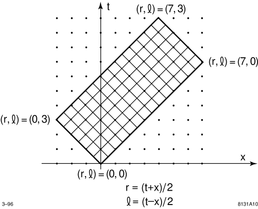
Figure 1: Rectangular lattice in Minkowski space-time.

We are thinking of $r$ and $\ell$ as the light cone coordinates $r=\frac{1}{2}\,(t+x)$, $\ell=\frac{1}{2}\,(t-x)$. Hence, in a standard diagram for Minkowski space-time, a pair of values $[r,\ell]$ determines a rectangle with sides of length $\ell$ and $r$ on the left and right pointing light cones. (We take the speed of light $c=1$.) This is shown in Figure. 1.

Clearly, the simplest way to think about this combinatorics is to take $\Delta=1$. If we wish to think about the usual continuum limit, then we shall fix values of $r$ and $\ell$ and choose $\Delta$ small but such that $r/\Delta$ and $\ell/\Delta$ are integers. The combinatorics of an $r\times\ell$ rectangle with integers $r$ and $\ell$ is no different in principle than the combinatorics of an $(r/\Delta)\times(\ell/\Delta)$ rectangle with integers $r/\Delta$ and $\ell/\Delta$. Accordingly, we shall take $\Delta=1$ for the rest of this discussion, and then make occasional comments to connect this with the general case.

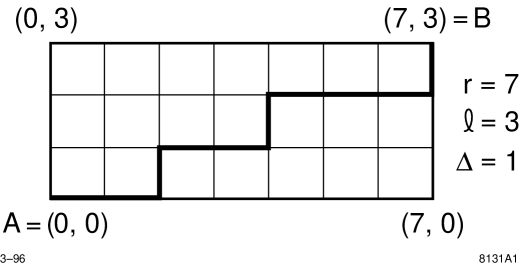
Figure 2: An example of a path in the light-cone rectangle.

Finally, for thinking about the combinatorics of the $r\times\ell$ rectangle, it is useful to view it turned by $45^{o}$ from its light-cone configuration. This is shown in Fig. 2. We shall consider lattice paths on the $r\times\ell$ rectangle from $A=[0,0]$ to $B=[r,\ell]$. Each step in such a path consists in an increment of either the first or the second light cone coordinate. The “particle” makes a series of “left or right” choices to get from A to B. In counting the lattice paths we shall represent left and right by

(Left is vertical in the rotated representation.) Now notice that a lattice path has two types of corners:

We can count RL corners by the point on the L axis where the path increments. We can count LR corners by the point on the R axis where the path increments. A lattice path is then determined by a choice of points from the L and R axes. More specifically, there are paths that begin in R (go right first) and end in L, begin in L and end in R, begin in L and end in L, begin in R and end in R. We call these paths of type RL, LR, LL and RR respectively. (Note that a RL corner is a two-step path of type RL and that an LR corner is a two step path of type LR.) It is easy to see that an RL path involves $k$ points from the R axis and $k+1$ points from the L axis, an LR path involves $k+1$ points from the R axis and k points from the L axis, while an LL or RR path involves the choice of $k$ points from each axis. See Figure 3 for examples.

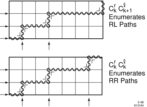
Figure 3: Showing by example that $C_{k}^{r}C_{k+1}^{\ell}$ enumerates RL paths and $C_{k}^{r}C_{k}^{\ell}$ enumerates RR paths.

As a consequence, we see that if $\|XY\|$ denotes the number of paths from A to B of type XY, then

$$\|RL\| = \Sigma_{k}C_{k}^{r}C_{k+1}^{\ell}$$

$$\|LR\| = \Sigma_{k}C_{k+1}^{r}C_{k}^{\ell}$$ (39)

$$\|RR\| = \|LL\|=\Sigma_{k}C_{k}^{r}C_{k}^{\ell}\ .$$

We see, therefore, that our functions $\psi_{0}$, $\psi_{R}$ and $\psi_{L}$ can be regarded as weighted sums over these different types of lattice path. In fact, we can re-interpret $(-)^{k}$ in terms of the number of corners (choices) in the paths:

$$RR \Rightarrow 2k\ \hbox{corners}$$

$$LR \Rightarrow 2k+1\ \hbox{corners}$$

$$RL \Rightarrow 2k+1\ \hbox{corners}$$

$$LL \Rightarrow 2k\ \hbox{corners}\ .$$

Hence if $N_{c}(XY)$ denotes the number of paths with $c$ corners of type XY then

$$\psi_{0} = \Sigma_{c}(-1)^{\frac{c}{2}}N_{c}(LL)=\Sigma_{c}(-1)^{\frac{c}{2}}\,N_{c}(RR)$$

$$\psi_{R} = \Sigma_{c}(-1)^{\frac{c-1}{2}}\,N_{c}(LR)$$ (40)

$$\psi_{L} = \Sigma_{c}(-1)^{\frac{c-1}{2}}\,N_{c}(RL)\ .$$

From the point of view of the solution to the RI Dirac equation ($\psi_{1}=\psi_{0}-\psi_{L}$, $\psi_{2}=\psi_{0}+\psi_{R}$) it is an interesting puzzle in discrete physics to understand the nature of the negative case counting that is entailed in the solution. (An attempt has been made by one of us to interpret this in terms of spin or particle number conservation in the presence of random electromagnetic fluctuations producing the paths [9].) The signs do not appear to come from local considerations along the path.

The RII Dirac solution gives a different point of view. Here $\psi_{1}=\psi_{0}-i\psi_{L}$, $\psi_{2}=\psi_{0}-i\psi_{R}$. Taken the hint given by the appearance of $i$, we note that $i^{2k}=(-)^{k}$ while $i^{2k+1}=(-1)^{k}i$. Thus

$$\psi_{1}=\Sigma_{c}(-i)^{c}N_{c}(R)\qquad\psi_{2}=\Sigma_{c}(-i)^{c}N_{c}(L)$$

where $N_{c}(R)$ denotes the number of paths that start to the right and have $c$ crossings, while $N_{c}(L)$ denotes the number of paths that start to the left and have $c$ crossings. This shows that our solution in the RII case is precisely in line with the amplitudes described by Feynman and Hibbs (Ref. [2]) for their checkerboard model of the Dirac propagator. See also H. A. Gersch [10] and Ref. [3] for the relationship of the Feynman model to the combinatorics of the Ising model in statistical mechanics.

Returning now to the RI equation, we see that $(-i)^{c}N_{c}$ gives the clue to the combinatorics of the signs. In our RI formulation, no complex numbers appear and none are needed if we take a combinatorial interpretation of $i$ as an operator on ordered pairs: $i[a,b]=[-b,a]$. Then we can think of a “pre-spinor” in the form of a labeled $\frac{\pi}{2}$ angle associated to each corner:

As the particle moves from corner to corner its pre-spinor is operated on by $i$. There is a combination of one sign change and one change in order. The total sign change from the beginning of the path to the end documents the positivity or negativity of the count.

5 Epilogue

If we had started by saying (in the RI case) we had a simple solution for the Dirac equation (discretized) using nothing but bit-strings (L,R choice sequences) and appropriate signs, then it would have been natural to ask: How are these signs justified on the basis of a philosophy of bit-strings? In retrospect we can answer: This pattern of signs is very simple, but not (yet) to be deduced from the notion of a distinction alone. Nevertheless, it does arise naturally from the simple structures that are available at that primitive level. The $i$ operator ($i[a,b]=[-b,a]$) does not involve anything more sophisticated that the idea of exchanging the labels on the two sides of a distinction followed by the flipping of a label on a given side:

as is discussed elsewhere [11, 12]. A choice sequence such as

has “corners” wherever R meets L or L meets R. We have characterized these corners into two types RL and LR:

We then enumerate the choice sequences in terms of lattice paths in Minkowski space and the solutions to the Dirac equation emerge, along with a precursor to spin and the role of $i=\sqrt{-1}$ in quantum mechanics. We have shown exactly how this point of view interfaces with Feynman’s Checkerboard.

Corners in the bit-string sequence alternate from RL to LR and from LR to RL. The moral of Feynman’s $(-i)^{c}$ where $c$ is the number of corners is that this alteration should be regarded as an elementary rotation:

One may wonder, why does this simple combinatorics occur in a level so close to the making of one distinction, and yet implicate fully the solutions to the Dirac equation in continuum 1+1 physics?! We cannot begin to answer such a question except with another question: If you believe that simple combinatorial principles underlie not only physics and physical law, but the generation of space-time herself, then these principles remain to be discovered. What are they? What are these principles? It is no surprise to the mathematician that $i$ ends up as central to the quest. For $i$ is a strange amphibian not only neither 1 nor $-1$, $i$ is neither discrete nor continuous, not algebra, not geometry, but a communicator of both. In this essay we have seen the beginning of a true connection of discrete and continuum physics.

The continuum version of our theory merges the paths on the lattice to a sum over all possible paths on an infinitely divided rectangle in Minkowski space-time. The individual paths disappear into the values of the series $\psi_{0}=\Sigma_{k=0}^{\infty}(-1)^{k}\frac{r^{k}}{k!}\,\frac{\ell^{k}}{k!}$, $\psi_{L}=\Sigma_{k=0}^{\infty}(-1)^{k}\frac{r^{k}}{k!}\,\frac{\ell^{k+1}}{(k+1)!}$ , $\psi_{R}=\Sigma_{k=0}^{\infty}(-1)^{k}\frac{r^{k+1}}{(k+1)!}\,\frac{\ell^{k}}{k!}$. Here we have a glimpse of the possibilities inherent in a complete story of discrete physics and its continuum limit. The continuum limit will be seen as a summary of the real physics. It is a way to view, through the glass darkly, the crystalline reality of simple quantum choice.

References

- [1] L. H. Kauffman and H. P. Noyes, “Discrete Physics and the Derivation of Electromagnetism from the Formalism of Quantum Mechanics,” Proceedings of the Royal Society A 452 (1996) 81-95 and references therein.
- [2] R. P. Feynman and A. R. Hibbs, Quantum Mechanics and Path Integrals, McGraw-Hill, New York 1965, Problem 2-6, pp 34-36.
- [3] T. Jacobson and L. S. Schulman, J. Phys. A: Math. Gen. 17 (1984) 375-383.
- [4] V. A. Karmanov Phys. Lett. A 174 (1993) 371.
- [5] T. Etter, “Process, System, Causality and Quantum Mechanics”, International Journal of General Systems, issue edited by K. Bowden on General systems and the Emergence of Physical Structure from Information Theory, (in press).
- [6] T. Etter, “The Final Collapse of the Wave Function” in Proceedings of ANPA WEST 12, F. Young, ed., ANPA WEST, 112 Blackburn Avenue, Menlo Park, CA 94025 (1996).
- [7] V. A. Karmanov, private communication to HPN, August 11, 1989.
- [8] E. Grey in Proceedings of ANPA 17, K. Bowden, ed.; available from C. W. Kilmister, Red Tiles Cottage, High Street, Barcombe, Lewes BN8 5DH, UK (September 1996).
- [9] H. P. Noyes, Physics Essays, 8 (1995) 434-445.
- [10] H. A. Gersch, Intl. J. Theor. Phys., 20 (1981) 491-501.
- [11] L. H. Kauffman, Knots and Physics, World Scientific, Singapore, 1991, 1994.
- [12] —, “Special Relativity and a Calculus of Distinctions”, in Discrete and Combinatorial Physics (Proceedings of ANPA 9), H. P. Noyes, ed., ANPA WEST, 112 Blackburn Avenue, Menlo Park, CA 94025 (1987) pp 290-311.
- [13] I. Stein, seminars at Stanford, 1978, 1979.
- [14] I. Stein, papers at the Second and Third Annual International Conferences of the Alternative Natural Philosophy Association, King’s College, Cambridge, 1980, 1981.
- [15] I. Stein, Physics Essays, 1 (1988) 155-170; 3 (1990) 66-70.
- [16] I. Stein, The Concept of Object as the Foundation of Physics, Peter Lang, New York (1996).