The Aharonov-Bohm scattering :
the role of the incident wave

Abstract

The scattering problem under the influence of the Aharonov-Bohm (AB) potential is reconsidered. By solving the Lippmann-Schwinger (LS) equation we obtain the wave function of the scattering state in this system. In spite of working with a plane wave as an incident wave we obtain the same wave function as was given by Aharonov and Bohm. Another method to solve the scattering problem is given by making use of a modified version of Gordon’s idea which was invented to consider the scattering by the Coulomb potential. These two methods give the same result, which guarantees the validity of taking an incident plane wave as usual to make an analysis of this scattering problem. The scattering problem by a solenoid of finite radius is also discussed, and we find that the vector potential of the solenoid affects the charged particles even when the magnitude of the flux is an odd integer as well as noninteger. It is shown that the unitarity of the $S$ matrix holds provided that a plane wave is taken to be an incident one.

Department of Physics, Hiyoshi, Keio University, Hiyoshi, Yokohama 223, Japan

1 Introduction

Since Aharonov and Bohm (AB) have discussed a scattering problem of a charged particle by a solenoid in order to clarify the significance of the vector potential in the quantum theory [1], many people have considered the same problem from various viewpoints [2]–[19]. As is well known, there are two approaches to deal with a scattering problem in the quantum theory. The first approach is to find a stationary state describing the scattering process by solving a time-independent Schrödinger equation. The second one is to study the time development of a wave packet with respect to a time-dependent Schrödinger equation. Most people as well as Aharonov and Bohm have analyzed the scattering by means of the first approach, and some people have discussed the same problem with the second approach [11], [19]. As we see in the following, however, in spite of these efforts it seems not to be clear what is an incident wave in this scattering process. In this paper we will try to answer this question with the first method because there seems to be lacking a common interpretation of the stationary wave function in the literature.

A system of charged particles interacting with the solenoid is described by a Hamiltonian

$$\hat{H}={1\over{2\mu}}\left\{{\hat{\leavevmode\mathchoice{\hbox{\rm tensysevensyfivesy\boldmath{$\displaystyle p$}}}{\hbox{\rm tensysevensyfivesy\boldmath{$\textstyle p$}}}{\hbox{\rm tensysevensyfivesy\boldmath{$\scriptstyle p$}}}{\hbox{\rm tensysevensyfivesy\boldmath{$\scriptscriptstyle p$}}}}-{e\over c}\leavevmode\mathchoice{\hbox{\rm tensysevensyfivesy\boldmath{$\displaystyle A$}}}{\hbox{\rm tensysevensyfivesy\boldmath{$\textstyle A$}}}{\hbox{\rm tensysevensyfivesy\boldmath{$\scriptstyle A$}}}{\hbox{\rm tensysevensyfivesy\boldmath{$\scriptscriptstyle A$}}}(\hat{\leavevmode\mathchoice{\hbox{\rm tensysevensyfivesy\boldmath{$\displaystyle x$}}}{\hbox{\rm tensysevensyfivesy\boldmath{$\textstyle x$}}}{\hbox{\rm tensysevensyfivesy\boldmath{$\scriptstyle x$}}}{\hbox{\rm tensysevensyfivesy\boldmath{$\scriptscriptstyle x$}}}})}\right\}^{2}\ ,$$ (1.1)

where the electromagnetic vector potential tensysevensyfivesy$\textstyle A$ is given by

$$\leavevmode\mathchoice{\hbox{\rm tensysevensyfivesy\boldmath{$\displaystyle A$}}}{\hbox{\rm tensysevensyfivesy\boldmath{$\textstyle A$}}}{\hbox{\rm tensysevensyfivesy\boldmath{$\scriptstyle A$}}}{\hbox{\rm tensysevensyfivesy\boldmath{$\scriptscriptstyle A$}}}(\leavevmode\mathchoice{\hbox{\rm tensysevensyfivesy\boldmath{$\displaystyle x$}}}{\hbox{\rm tensysevensyfivesy\boldmath{$\textstyle x$}}}{\hbox{\rm tensysevensyfivesy\boldmath{$\scriptstyle x$}}}{\hbox{\rm tensysevensyfivesy\boldmath{$\scriptscriptstyle x$}}})={\Phi\over 2\pi r}\left(-\sin\varphi,\cos\varphi\right),\qquad(x,y)=(r\cos\varphi,r\sin\varphi).$$

In order to study the scattering of the charged particles we solve the time-independent Schrödinger equation

$$\hat{H}\psi_{E}(r,\varphi)=E\psi_{E}(r,\varphi)$$ (1.2)

to find an eigenfunction which describes the scattering process of charged particles.

Since the Hamiltonian commutes with the angular momentum, it can be easily shown that a most general solution of (1.2) is given by

$$\psi_{E}(r,\varphi)=\sum_{n=-\infty}^{+\infty}c_{n}e^{in\varphi}J_{|n+\alpha|}(kr),\ E={(\hbar k)^{2}\over 2\mu},$$ (1.3)

where $J_{\nu}(x)$ denotes the Bessel function of $\nu$-th order and we have put $\alpha=-e\Phi/2\pi\hbar c$. In (1.3), $c_{n}$’s are arbitrary constants to be determined by phisycal requirements. Our main interest here and in the following is to ask what should be the correct choice for the coefficients $c_{n}$’s to describe the scattering process.

It has been asserted by Aharonov and Bohm and many other authors that the incident wave for this scattering problem, when the incident beam comes into from the positive $x$ axis, should be a modulated plane wave $e^{-ikr\cos\varphi-i\alpha\varphi}$ to make the probability current of the incident wave constant. To fulfill this requirement the coefficients have been taken to be $c_{n}=(-i)^{|n+\alpha|}$. In the case of nonintegral $\alpha$, however, the incident wave becomes a multi-valued function. We may say that from the physical point of view it seems quite unsatisfactory to take such a multi-valued wave function as an incident one. We should also note that, for sufficiently large $r$, the term due to the vector potential do not contribute to the dominant part of the current, even if we take a plane wave as an incident wave function. Thus, it is not conclusive to argue that the incident modulated wave gives the condition to determine those constants as $c_{n}=(-i)^{|n+\alpha|}$.

It will be, therefore, instructive to reconsider the scattering problem from other viewpoints. In this paper we try to find the wave function to describe the scattering process using two different ways. The first one is to solve the Lippmann-Schwinger (LS) equation, which will be a standard method to consider the scattering problem of a quantum system, taking a plane wave as an incident state instead of the modulated one. If we adopt the Born expansion to solve the LS equation, we will soon meet a difficulty because the perturbative method does not work for the present problem as is shown in [15], [16]. Then we find an exact solution of the LS equation with the aid of the Feynman kernel. The second method is an application of Gordon’s idea which is proposed to discuss the scattering problem by the Coulomb potential [13]. The idea may have been introduced to avoid the difficulty caused by the long-ranged nature of the Coulomb potential in formulating a scattering theory. This method will also be useful to examine scattering problems by other potentials with long-range effect. It will be shown that these two methods give the same wave function to describe the scattering state given by AB [1].

If $\alpha=\mathchoice{\hbox{\rm integer}}{\hbox{\rm integer}}{\hbox{\rm integer}}{\hbox{\rm integer}}$, a further discussion is needed since the solution of the Schrödinger equation for infinitely thin solenoid does neither vanish nor be defined at the origin in that case. To ensure the impenetrability of the solenoid even for integral $\alpha$, we assume a solenoid to have a finite radius and consider this issue by generalizing the second method.

The plan of this paper is as follows. In section 2 we give the Feynman kernel with effects of the solenoid potential using the path integral method. Section 3 is devoted to solving the LS equation exactly with the aid of the Feynman kernel, and the explicit form of the wave function will be obtained. In section 4 Gordon’s method will be argued and its generalization to a system of a solenoid with finite radius will be done in section 5. Conclusions and discussions in comparison with other’s results are made in section 6.

2 The Feynman kernel with effects of the solenoid potential

Since the complete set of the eigenfunctions

$${1\over\sqrt{2\pi}}e^{in\varphi}J_{|n+\alpha|}(kr),\qquad n=0,\pm 1,\pm 2,\ldots$$

for the Hamiltonian with effects of the solenoid are known, we can immediately find an expression of the Feynman kernel

$$K(\leavevmode\mathchoice{\hbox{\rm tensysevensyfivesy\boldmath{$\displaystyle x$}}}{\hbox{\rm tensysevensyfivesy\boldmath{$\textstyle x$}}}{\hbox{\rm tensysevensyfivesy\boldmath{$\scriptstyle x$}}}{\hbox{\rm tensysevensyfivesy\boldmath{$\scriptscriptstyle x$}}}_{F},\leavevmode\mathchoice{\hbox{\rm tensysevensyfivesy\boldmath{$\displaystyle x$}}}{\hbox{\rm tensysevensyfivesy\boldmath{$\textstyle x$}}}{\hbox{\rm tensysevensyfivesy\boldmath{$\scriptstyle x$}}}{\hbox{\rm tensysevensyfivesy\boldmath{$\scriptscriptstyle x$}}}_{I};T)=\langle\leavevmode\mathchoice{\hbox{\rm tensysevensyfivesy\boldmath{$\displaystyle x$}}}{\hbox{\rm tensysevensyfivesy\boldmath{$\textstyle x$}}}{\hbox{\rm tensysevensyfivesy\boldmath{$\scriptstyle x$}}}{\hbox{\rm tensysevensyfivesy\boldmath{$\scriptscriptstyle x$}}}_{F}|e^{-i\hat{H}T/\hbar}|\leavevmode\mathchoice{\hbox{\rm tensysevensyfivesy\boldmath{$\displaystyle x$}}}{\hbox{\rm tensysevensyfivesy\boldmath{$\textstyle x$}}}{\hbox{\rm tensysevensyfivesy\boldmath{$\scriptstyle x$}}}{\hbox{\rm tensysevensyfivesy\boldmath{$\scriptscriptstyle x$}}}_{I}\rangle$$ (2.1)

as its spectral representation [6], [11]

$$K(\leavevmode\mathchoice{\hbox{\rm tensysevensyfivesy\boldmath{$\displaystyle x$}}}{\hbox{\rm tensysevensyfivesy\boldmath{$\textstyle x$}}}{\hbox{\rm tensysevensyfivesy\boldmath{$\scriptstyle x$}}}{\hbox{\rm tensysevensyfivesy\boldmath{$\scriptscriptstyle x$}}}_{F},\leavevmode\mathchoice{\hbox{\rm tensysevensyfivesy\boldmath{$\displaystyle x$}}}{\hbox{\rm tensysevensyfivesy\boldmath{$\textstyle x$}}}{\hbox{\rm tensysevensyfivesy\boldmath{$\scriptstyle x$}}}{\hbox{\rm tensysevensyfivesy\boldmath{$\scriptscriptstyle x$}}}_{I};T)=\int_{0}^{\infty}kdke^{-i\hbar k^{2}T/2\mu}{1\over 2\pi}\sum_{n=-\infty}^{+\infty}e^{in(\varphi_{F}-\varphi_{I})}J_{|n+\alpha|}(kr_{F})J_{|n+\alpha|}(kr_{I}).$$ (2.2)

To verify this expression, it suffices to notice the following facts, (i) it obeys the time-dependent Schrödinger equation, (ii) it is apparently single-valued with respect to both $\leavevmode\mathchoice{\hbox{\rm tensysevensyfivesy\boldmath{$\displaystyle x$}}}{\hbox{\rm tensysevensyfivesy\boldmath{$\textstyle x$}}}{\hbox{\rm tensysevensyfivesy\boldmath{$\scriptstyle x$}}}{\hbox{\rm tensysevensyfivesy\boldmath{$\scriptscriptstyle x$}}}_{F}$ and $\leavevmode\mathchoice{\hbox{\rm tensysevensyfivesy\boldmath{$\displaystyle x$}}}{\hbox{\rm tensysevensyfivesy\boldmath{$\textstyle x$}}}{\hbox{\rm tensysevensyfivesy\boldmath{$\scriptstyle x$}}}{\hbox{\rm tensysevensyfivesy\boldmath{$\scriptscriptstyle x$}}}_{I}$, (iii) it has the correct limit

$$\lim\limits_{t\rightarrow 0}K(\leavevmode\mathchoice{\hbox{\rm tensysevensyfivesy\boldmath{$\displaystyle x$}}}{\hbox{\rm tensysevensyfivesy\boldmath{$\textstyle x$}}}{\hbox{\rm tensysevensyfivesy\boldmath{$\scriptstyle x$}}}{\hbox{\rm tensysevensyfivesy\boldmath{$\scriptscriptstyle x$}}}_{F},\leavevmode\mathchoice{\hbox{\rm tensysevensyfivesy\boldmath{$\displaystyle x$}}}{\hbox{\rm tensysevensyfivesy\boldmath{$\textstyle x$}}}{\hbox{\rm tensysevensyfivesy\boldmath{$\scriptstyle x$}}}{\hbox{\rm tensysevensyfivesy\boldmath{$\scriptscriptstyle x$}}}_{I};t)=\delta^{2}(\leavevmode\mathchoice{\hbox{\rm tensysevensyfivesy\boldmath{$\displaystyle x$}}}{\hbox{\rm tensysevensyfivesy\boldmath{$\textstyle x$}}}{\hbox{\rm tensysevensyfivesy\boldmath{$\scriptstyle x$}}}{\hbox{\rm tensysevensyfivesy\boldmath{$\scriptscriptstyle x$}}}_{F}-\leavevmode\mathchoice{\hbox{\rm tensysevensyfivesy\boldmath{$\displaystyle x$}}}{\hbox{\rm tensysevensyfivesy\boldmath{$\textstyle x$}}}{\hbox{\rm tensysevensyfivesy\boldmath{$\scriptstyle x$}}}{\hbox{\rm tensysevensyfivesy\boldmath{$\scriptscriptstyle x$}}}_{I}),$$ (2.3)

which follows from

$${1\over\sqrt{ab}}\delta(a-b)=\int_{0}^{\infty}kdkJ_{\nu}(ak)J_{\nu}(bk)\qquad[\mathchoice{\hbox{\rm Re}}{\hbox{\rm Re}}{\hbox{\rm Re}}{\hbox{\rm Re}}(\nu)>-1,\ a,b>0]\ ,$$ (2.4)

and

$$\sum_{n=-\infty}^{+\infty}e^{in\theta}=2\pi\delta(\theta)\qquad[-\pi<\theta<\pi]\ .$$ (2.5)

If we carry out the integration with respect to $k$ in (2.2), we obtain

$$K(\leavevmode\mathchoice{\hbox{\rm tensysevensyfivesy\boldmath{$\displaystyle x$}}}{\hbox{\rm tensysevensyfivesy\boldmath{$\textstyle x$}}}{\hbox{\rm tensysevensyfivesy\boldmath{$\scriptstyle x$}}}{\hbox{\rm tensysevensyfivesy\boldmath{$\scriptscriptstyle x$}}}_{F},\leavevmode\mathchoice{\hbox{\rm tensysevensyfivesy\boldmath{$\displaystyle x$}}}{\hbox{\rm tensysevensyfivesy\boldmath{$\textstyle x$}}}{\hbox{\rm tensysevensyfivesy\boldmath{$\scriptstyle x$}}}{\hbox{\rm tensysevensyfivesy\boldmath{$\scriptscriptstyle x$}}}_{I};T)={\mu\over 2\pi i\hbar T}\sum_{n=-\infty}^{+\infty}\exp\left\{{i\mu\over 2\hbar T}(r^{2}+r^{\prime}{}^{2})\right\}I_{|n+\alpha|}\left({\mu rr^{\prime}\over i\hbar T}\right)e^{in(\varphi-\varphi^{\prime})}\ .$$ (2.6)

By use of (2.2) or (2.6) we can proceed to solve the LS equation. In this section, however, we would like to give another derivation of (2.2) because there seems to be some confusion in the path integral construction of the Feynman kernel in the literature [7]–[10]. Among them the most typical one would be the interpretation of its expression as the sum over winding number such as

$$K(\leavevmode\mathchoice{\hbox{\rm tensysevensyfivesy\boldmath{$\displaystyle x$}}}{\hbox{\rm tensysevensyfivesy\boldmath{$\textstyle x$}}}{\hbox{\rm tensysevensyfivesy\boldmath{$\scriptstyle x$}}}{\hbox{\rm tensysevensyfivesy\boldmath{$\scriptscriptstyle x$}}}_{F},\leavevmode\mathchoice{\hbox{\rm tensysevensyfivesy\boldmath{$\displaystyle x$}}}{\hbox{\rm tensysevensyfivesy\boldmath{$\textstyle x$}}}{\hbox{\rm tensysevensyfivesy\boldmath{$\scriptstyle x$}}}{\hbox{\rm tensysevensyfivesy\boldmath{$\scriptscriptstyle x$}}}_{I};T)=\sum_{m=-\infty}^{+\infty}e^{-i\alpha(\varphi_{F}-\varphi_{I}-2m\pi)}K_{m}(\leavevmode\mathchoice{\hbox{\rm tensysevensyfivesy\boldmath{$\displaystyle x$}}}{\hbox{\rm tensysevensyfivesy\boldmath{$\textstyle x$}}}{\hbox{\rm tensysevensyfivesy\boldmath{$\scriptstyle x$}}}{\hbox{\rm tensysevensyfivesy\boldmath{$\scriptscriptstyle x$}}}_{F},\leavevmode\mathchoice{\hbox{\rm tensysevensyfivesy\boldmath{$\displaystyle x$}}}{\hbox{\rm tensysevensyfivesy\boldmath{$\textstyle x$}}}{\hbox{\rm tensysevensyfivesy\boldmath{$\scriptstyle x$}}}{\hbox{\rm tensysevensyfivesy\boldmath{$\scriptscriptstyle x$}}}_{I};T),$$ (2.7)

where $K_{m}(\leavevmode\mathchoice{\hbox{\rm tensysevensyfivesy\boldmath{$\displaystyle x$}}}{\hbox{\rm tensysevensyfivesy\boldmath{$\textstyle x$}}}{\hbox{\rm tensysevensyfivesy\boldmath{$\scriptstyle x$}}}{\hbox{\rm tensysevensyfivesy\boldmath{$\scriptscriptstyle x$}}}_{F},\leavevmode\mathchoice{\hbox{\rm tensysevensyfivesy\boldmath{$\displaystyle x$}}}{\hbox{\rm tensysevensyfivesy\boldmath{$\textstyle x$}}}{\hbox{\rm tensysevensyfivesy\boldmath{$\scriptstyle x$}}}{\hbox{\rm tensysevensyfivesy\boldmath{$\scriptscriptstyle x$}}}_{I};T)$ comes from paths going around the solenoid $m$ times in anticlockwise way, and the factor $e^{2\pi im\alpha}$ is a one dimensional representation of the fundamental group of the configuration space. In the following, however, we show that the sum over winding number is not essential, and that the sum in (2.7) is to be interpreted as a result of the reformulation with aid of the Poisson sum formula for the expression obtained using the usual path integral method. To achieve this we will make use of the completeness relations of both eigenvectors $|\leavevmode\mathchoice{\hbox{\rm tensysevensyfivesy\boldmath{$\displaystyle x$}}}{\hbox{\rm tensysevensyfivesy\boldmath{$\textstyle x$}}}{\hbox{\rm tensysevensyfivesy\boldmath{$\scriptstyle x$}}}{\hbox{\rm tensysevensyfivesy\boldmath{$\scriptscriptstyle x$}}}\rangle$ of $\hat{\leavevmode\mathchoice{\hbox{\rm tensysevensyfivesy\boldmath{$\displaystyle x$}}}{\hbox{\rm tensysevensyfivesy\boldmath{$\textstyle x$}}}{\hbox{\rm tensysevensyfivesy\boldmath{$\scriptstyle x$}}}{\hbox{\rm tensysevensyfivesy\boldmath{$\scriptscriptstyle x$}}}}$ with eigenvalue tensysevensyfivesy$\textstyle x$, and eigenvectors $|\leavevmode\mathchoice{\hbox{\rm tensysevensyfivesy\boldmath{$\displaystyle p$}}}{\hbox{\rm tensysevensyfivesy\boldmath{$\textstyle p$}}}{\hbox{\rm tensysevensyfivesy\boldmath{$\scriptstyle p$}}}{\hbox{\rm tensysevensyfivesy\boldmath{$\scriptscriptstyle p$}}}\rangle$ of $\hat{\leavevmode\mathchoice{\hbox{\rm tensysevensyfivesy\boldmath{$\displaystyle p$}}}{\hbox{\rm tensysevensyfivesy\boldmath{$\textstyle p$}}}{\hbox{\rm tensysevensyfivesy\boldmath{$\scriptstyle p$}}}{\hbox{\rm tensysevensyfivesy\boldmath{$\scriptscriptstyle p$}}}}$ with eigenvalue tensysevensyfivesy$\textstyle p$, in formulating the path integral. As is easily recognized, the single-valuedness of (2.7) is the consequence of these relations [12].

Now we give the path integral derivation for the Feynman kernel of this system. Defining the exponential operator by

$$e^{-i\hat{H}T/\hbar}=\lim\limits_{N\rightarrow\infty}\left(1-{i\varepsilon\over\hbar}\hat{H}\right)^{N},\qquad\varepsilon=T/N,$$ (2.8)

and using the completeness of the states $|\leavevmode\mathchoice{\hbox{\rm tensysevensyfivesy\boldmath{$\displaystyle x$}}}{\hbox{\rm tensysevensyfivesy\boldmath{$\textstyle x$}}}{\hbox{\rm tensysevensyfivesy\boldmath{$\scriptstyle x$}}}{\hbox{\rm tensysevensyfivesy\boldmath{$\scriptscriptstyle x$}}}\rangle$, we obtain

$$K(\leavevmode\mathchoice{\hbox{\rm tensysevensyfivesy\boldmath{$\displaystyle x$}}}{\hbox{\rm tensysevensyfivesy\boldmath{$\textstyle x$}}}{\hbox{\rm tensysevensyfivesy\boldmath{$\scriptstyle x$}}}{\hbox{\rm tensysevensyfivesy\boldmath{$\scriptscriptstyle x$}}}_{F},\leavevmode\mathchoice{\hbox{\rm tensysevensyfivesy\boldmath{$\displaystyle x$}}}{\hbox{\rm tensysevensyfivesy\boldmath{$\textstyle x$}}}{\hbox{\rm tensysevensyfivesy\boldmath{$\scriptstyle x$}}}{\hbox{\rm tensysevensyfivesy\boldmath{$\scriptscriptstyle x$}}}_{I};T)=\lim\limits_{N\rightarrow\infty}\int\prod_{i=1}^{N-1}{d^{2}x(i)}\prod_{j=1}^{N}\langle\leavevmode\mathchoice{\hbox{\rm tensysevensyfivesy\boldmath{$\displaystyle x$}}}{\hbox{\rm tensysevensyfivesy\boldmath{$\textstyle x$}}}{\hbox{\rm tensysevensyfivesy\boldmath{$\scriptstyle x$}}}{\hbox{\rm tensysevensyfivesy\boldmath{$\scriptscriptstyle x$}}}(j)|\left(1-{i\varepsilon\over\hbar}\hat{H}\right)|\leavevmode\mathchoice{\hbox{\rm tensysevensyfivesy\boldmath{$\displaystyle x$}}}{\hbox{\rm tensysevensyfivesy\boldmath{$\textstyle x$}}}{\hbox{\rm tensysevensyfivesy\boldmath{$\scriptstyle x$}}}{\hbox{\rm tensysevensyfivesy\boldmath{$\scriptscriptstyle x$}}}(j-1)\rangle.$$ (2.9)

Then, with the aid of the completeness of the states $|\leavevmode\mathchoice{\hbox{\rm tensysevensyfivesy\boldmath{$\displaystyle p$}}}{\hbox{\rm tensysevensyfivesy\boldmath{$\textstyle p$}}}{\hbox{\rm tensysevensyfivesy\boldmath{$\scriptstyle p$}}}{\hbox{\rm tensysevensyfivesy\boldmath{$\scriptscriptstyle p$}}}\rangle$, we can express the infinitesimal version of the Feynman kernel as

$$\langle\leavevmode\mathchoice{\hbox{\rm tensysevensyfivesy\boldmath{$\displaystyle x$}}}{\hbox{\rm tensysevensyfivesy\boldmath{$\textstyle x$}}}{\hbox{\rm tensysevensyfivesy\boldmath{$\scriptstyle x$}}}{\hbox{\rm tensysevensyfivesy\boldmath{$\scriptscriptstyle x$}}}|\left(1-{i\varepsilon\over\hbar}\hat{H}\right)|\leavevmode\mathchoice{\hbox{\rm tensysevensyfivesy\boldmath{$\displaystyle x$}}}{\hbox{\rm tensysevensyfivesy\boldmath{$\textstyle x$}}}{\hbox{\rm tensysevensyfivesy\boldmath{$\scriptstyle x$}}}{\hbox{\rm tensysevensyfivesy\boldmath{$\scriptscriptstyle x$}}}^{\prime}\rangle$$ (2.10)

$$= \lim\limits_{\delta\rightarrow 0}\int{d^{2}p\over(2\pi\hbar)^{2}}\exp\left\{{i\over\hbar}\leavevmode\mathchoice{\hbox{\rm tensysevensyfivesy\boldmath{$\displaystyle p$}}}{\hbox{\rm tensysevensyfivesy\boldmath{$\textstyle p$}}}{\hbox{\rm tensysevensyfivesy\boldmath{$\scriptstyle p$}}}{\hbox{\rm tensysevensyfivesy\boldmath{$\scriptscriptstyle p$}}}(\leavevmode\mathchoice{\hbox{\rm tensysevensyfivesy\boldmath{$\displaystyle x$}}}{\hbox{\rm tensysevensyfivesy\boldmath{$\textstyle x$}}}{\hbox{\rm tensysevensyfivesy\boldmath{$\scriptstyle x$}}}{\hbox{\rm tensysevensyfivesy\boldmath{$\scriptscriptstyle x$}}}-\leavevmode\mathchoice{\hbox{\rm tensysevensyfivesy\boldmath{$\displaystyle x$}}}{\hbox{\rm tensysevensyfivesy\boldmath{$\textstyle x$}}}{\hbox{\rm tensysevensyfivesy\boldmath{$\scriptstyle x$}}}{\hbox{\rm tensysevensyfivesy\boldmath{$\scriptscriptstyle x$}}}^{\prime})-{\delta\over 2}\leavevmode\mathchoice{\hbox{\rm tensysevensyfivesy\boldmath{$\displaystyle p$}}}{\hbox{\rm tensysevensyfivesy\boldmath{$\textstyle p$}}}{\hbox{\rm tensysevensyfivesy\boldmath{$\scriptstyle p$}}}{\hbox{\rm tensysevensyfivesy\boldmath{$\scriptscriptstyle p$}}}^{2}\right\}\left[1-{i\varepsilon\over\hbar}{1\over{2\mu}}\left\{{\leavevmode\mathchoice{\hbox{\rm tensysevensyfivesy\boldmath{$\displaystyle p$}}}{\hbox{\rm tensysevensyfivesy\boldmath{$\textstyle p$}}}{\hbox{\rm tensysevensyfivesy\boldmath{$\scriptstyle p$}}}{\hbox{\rm tensysevensyfivesy\boldmath{$\scriptscriptstyle p$}}}-{e\over c}\overline{\leavevmode\mathchoice{\hbox{\rm tensysevensyfivesy\boldmath{$\displaystyle A$}}}{\hbox{\rm tensysevensyfivesy\boldmath{$\textstyle A$}}}{\hbox{\rm tensysevensyfivesy\boldmath{$\scriptstyle A$}}}{\hbox{\rm tensysevensyfivesy\boldmath{$\scriptscriptstyle A$}}}}(\leavevmode\mathchoice{\hbox{\rm tensysevensyfivesy\boldmath{$\displaystyle x$}}}{\hbox{\rm tensysevensyfivesy\boldmath{$\textstyle x$}}}{\hbox{\rm tensysevensyfivesy\boldmath{$\scriptstyle x$}}}{\hbox{\rm tensysevensyfivesy\boldmath{$\scriptscriptstyle x$}}},\leavevmode\mathchoice{\hbox{\rm tensysevensyfivesy\boldmath{$\displaystyle x$}}}{\hbox{\rm tensysevensyfivesy\boldmath{$\textstyle x$}}}{\hbox{\rm tensysevensyfivesy\boldmath{$\scriptstyle x$}}}{\hbox{\rm tensysevensyfivesy\boldmath{$\scriptscriptstyle x$}}}^{\prime})}\right\}^{2}\right]\ ,$$

where $\overline{\leavevmode\mathchoice{\hbox{\rm tensysevensyfivesy\boldmath{$\displaystyle A$}}}{\hbox{\rm tensysevensyfivesy\boldmath{$\textstyle A$}}}{\hbox{\rm tensysevensyfivesy\boldmath{$\scriptstyle A$}}}{\hbox{\rm tensysevensyfivesy\boldmath{$\scriptscriptstyle A$}}}}(\leavevmode\mathchoice{\hbox{\rm tensysevensyfivesy\boldmath{$\displaystyle x$}}}{\hbox{\rm tensysevensyfivesy\boldmath{$\textstyle x$}}}{\hbox{\rm tensysevensyfivesy\boldmath{$\scriptstyle x$}}}{\hbox{\rm tensysevensyfivesy\boldmath{$\scriptscriptstyle x$}}},\leavevmode\mathchoice{\hbox{\rm tensysevensyfivesy\boldmath{$\displaystyle x$}}}{\hbox{\rm tensysevensyfivesy\boldmath{$\textstyle x$}}}{\hbox{\rm tensysevensyfivesy\boldmath{$\scriptstyle x$}}}{\hbox{\rm tensysevensyfivesy\boldmath{$\scriptscriptstyle x$}}}^{\prime})=\{\leavevmode\mathchoice{\hbox{\rm tensysevensyfivesy\boldmath{$\displaystyle A$}}}{\hbox{\rm tensysevensyfivesy\boldmath{$\textstyle A$}}}{\hbox{\rm tensysevensyfivesy\boldmath{$\scriptstyle A$}}}{\hbox{\rm tensysevensyfivesy\boldmath{$\scriptscriptstyle A$}}}(\leavevmode\mathchoice{\hbox{\rm tensysevensyfivesy\boldmath{$\displaystyle x$}}}{\hbox{\rm tensysevensyfivesy\boldmath{$\textstyle x$}}}{\hbox{\rm tensysevensyfivesy\boldmath{$\scriptstyle x$}}}{\hbox{\rm tensysevensyfivesy\boldmath{$\scriptscriptstyle x$}}})+\leavevmode\mathchoice{\hbox{\rm tensysevensyfivesy\boldmath{$\displaystyle A$}}}{\hbox{\rm tensysevensyfivesy\boldmath{$\textstyle A$}}}{\hbox{\rm tensysevensyfivesy\boldmath{$\scriptstyle A$}}}{\hbox{\rm tensysevensyfivesy\boldmath{$\scriptscriptstyle A$}}}(\leavevmode\mathchoice{\hbox{\rm tensysevensyfivesy\boldmath{$\displaystyle x$}}}{\hbox{\rm tensysevensyfivesy\boldmath{$\textstyle x$}}}{\hbox{\rm tensysevensyfivesy\boldmath{$\scriptstyle x$}}}{\hbox{\rm tensysevensyfivesy\boldmath{$\scriptscriptstyle x$}}}^{\prime})\}/2$.

After shifting the integration variable tensysevensyfivesy$\textstyle p$ by

$$\leavevmode\mathchoice{\hbox{\rm tensysevensyfivesy\boldmath{$\displaystyle p$}}}{\hbox{\rm tensysevensyfivesy\boldmath{$\textstyle p$}}}{\hbox{\rm tensysevensyfivesy\boldmath{$\scriptstyle p$}}}{\hbox{\rm tensysevensyfivesy\boldmath{$\scriptscriptstyle p$}}}\mapsto\leavevmode\mathchoice{\hbox{\rm tensysevensyfivesy\boldmath{$\displaystyle p$}}}{\hbox{\rm tensysevensyfivesy\boldmath{$\textstyle p$}}}{\hbox{\rm tensysevensyfivesy\boldmath{$\scriptstyle p$}}}{\hbox{\rm tensysevensyfivesy\boldmath{$\scriptscriptstyle p$}}}+{e\over c}\overline{\leavevmode\mathchoice{\hbox{\rm tensysevensyfivesy\boldmath{$\displaystyle A$}}}{\hbox{\rm tensysevensyfivesy\boldmath{$\textstyle A$}}}{\hbox{\rm tensysevensyfivesy\boldmath{$\scriptstyle A$}}}{\hbox{\rm tensysevensyfivesy\boldmath{$\scriptscriptstyle A$}}}}(\leavevmode\mathchoice{\hbox{\rm tensysevensyfivesy\boldmath{$\displaystyle x$}}}{\hbox{\rm tensysevensyfivesy\boldmath{$\textstyle x$}}}{\hbox{\rm tensysevensyfivesy\boldmath{$\scriptstyle x$}}}{\hbox{\rm tensysevensyfivesy\boldmath{$\scriptscriptstyle x$}}},\leavevmode\mathchoice{\hbox{\rm tensysevensyfivesy\boldmath{$\displaystyle x$}}}{\hbox{\rm tensysevensyfivesy\boldmath{$\textstyle x$}}}{\hbox{\rm tensysevensyfivesy\boldmath{$\scriptstyle x$}}}{\hbox{\rm tensysevensyfivesy\boldmath{$\scriptscriptstyle x$}}}^{\prime}),$$

we can rewrite (2.10) as

$$\langle\leavevmode\mathchoice{\hbox{\rm tensysevensyfivesy\boldmath{$\displaystyle x$}}}{\hbox{\rm tensysevensyfivesy\boldmath{$\textstyle x$}}}{\hbox{\rm tensysevensyfivesy\boldmath{$\scriptstyle x$}}}{\hbox{\rm tensysevensyfivesy\boldmath{$\scriptscriptstyle x$}}}|\left(1-{i\varepsilon\over\hbar}\hat{H}\right)|\leavevmode\mathchoice{\hbox{\rm tensysevensyfivesy\boldmath{$\displaystyle x$}}}{\hbox{\rm tensysevensyfivesy\boldmath{$\textstyle x$}}}{\hbox{\rm tensysevensyfivesy\boldmath{$\scriptstyle x$}}}{\hbox{\rm tensysevensyfivesy\boldmath{$\scriptscriptstyle x$}}}^{\prime}\rangle = \exp\left\{{{ie\over\hbar c}\overline{\leavevmode\mathchoice{\hbox{\rm tensysevensyfivesy\boldmath{$\displaystyle A$}}}{\hbox{\rm tensysevensyfivesy\boldmath{$\textstyle A$}}}{\hbox{\rm tensysevensyfivesy\boldmath{$\scriptstyle A$}}}{\hbox{\rm tensysevensyfivesy\boldmath{$\scriptscriptstyle A$}}}}(\leavevmode\mathchoice{\hbox{\rm tensysevensyfivesy\boldmath{$\displaystyle x$}}}{\hbox{\rm tensysevensyfivesy\boldmath{$\textstyle x$}}}{\hbox{\rm tensysevensyfivesy\boldmath{$\scriptstyle x$}}}{\hbox{\rm tensysevensyfivesy\boldmath{$\scriptscriptstyle x$}}},\leavevmode\mathchoice{\hbox{\rm tensysevensyfivesy\boldmath{$\displaystyle x$}}}{\hbox{\rm tensysevensyfivesy\boldmath{$\textstyle x$}}}{\hbox{\rm tensysevensyfivesy\boldmath{$\scriptstyle x$}}}{\hbox{\rm tensysevensyfivesy\boldmath{$\scriptscriptstyle x$}}}^{\prime})(\leavevmode\mathchoice{\hbox{\rm tensysevensyfivesy\boldmath{$\displaystyle x$}}}{\hbox{\rm tensysevensyfivesy\boldmath{$\textstyle x$}}}{\hbox{\rm tensysevensyfivesy\boldmath{$\scriptstyle x$}}}{\hbox{\rm tensysevensyfivesy\boldmath{$\scriptscriptstyle x$}}}-\leavevmode\mathchoice{\hbox{\rm tensysevensyfivesy\boldmath{$\displaystyle x$}}}{\hbox{\rm tensysevensyfivesy\boldmath{$\textstyle x$}}}{\hbox{\rm tensysevensyfivesy\boldmath{$\scriptstyle x$}}}{\hbox{\rm tensysevensyfivesy\boldmath{$\scriptscriptstyle x$}}}^{\prime})}\right\}$$ (2.11)

$$\times\lim\limits_{\delta\rightarrow 0}\int{d^{2}p\over(2\pi\hbar)^{2}}\exp\left\{{i\over\hbar}\leavevmode\mathchoice{\hbox{\rm tensysevensyfivesy\boldmath{$\displaystyle p$}}}{\hbox{\rm tensysevensyfivesy\boldmath{$\textstyle p$}}}{\hbox{\rm tensysevensyfivesy\boldmath{$\scriptstyle p$}}}{\hbox{\rm tensysevensyfivesy\boldmath{$\scriptscriptstyle p$}}}(\leavevmode\mathchoice{\hbox{\rm tensysevensyfivesy\boldmath{$\displaystyle x$}}}{\hbox{\rm tensysevensyfivesy\boldmath{$\textstyle x$}}}{\hbox{\rm tensysevensyfivesy\boldmath{$\scriptstyle x$}}}{\hbox{\rm tensysevensyfivesy\boldmath{$\scriptscriptstyle x$}}}-\leavevmode\mathchoice{\hbox{\rm tensysevensyfivesy\boldmath{$\displaystyle x$}}}{\hbox{\rm tensysevensyfivesy\boldmath{$\textstyle x$}}}{\hbox{\rm tensysevensyfivesy\boldmath{$\scriptstyle x$}}}{\hbox{\rm tensysevensyfivesy\boldmath{$\scriptscriptstyle x$}}}^{\prime})-{1\over 2}\left(\delta+{i\varepsilon\over\hbar\mu}\right)\leavevmode\mathchoice{\hbox{\rm tensysevensyfivesy\boldmath{$\displaystyle p$}}}{\hbox{\rm tensysevensyfivesy\boldmath{$\textstyle p$}}}{\hbox{\rm tensysevensyfivesy\boldmath{$\scriptstyle p$}}}{\hbox{\rm tensysevensyfivesy\boldmath{$\scriptscriptstyle p$}}}^{2}\right\}\ .$$

Carrying out the Gaussian integration with respect to tensysevensyfivesy$\textstyle p$ and noting that

$$\overline{\leavevmode\mathchoice{\hbox{\rm tensysevensyfivesy\boldmath{$\displaystyle A$}}}{\hbox{\rm tensysevensyfivesy\boldmath{$\textstyle A$}}}{\hbox{\rm tensysevensyfivesy\boldmath{$\scriptstyle A$}}}{\hbox{\rm tensysevensyfivesy\boldmath{$\scriptscriptstyle A$}}}}(\leavevmode\mathchoice{\hbox{\rm tensysevensyfivesy\boldmath{$\displaystyle x$}}}{\hbox{\rm tensysevensyfivesy\boldmath{$\textstyle x$}}}{\hbox{\rm tensysevensyfivesy\boldmath{$\scriptstyle x$}}}{\hbox{\rm tensysevensyfivesy\boldmath{$\scriptscriptstyle x$}}},\leavevmode\mathchoice{\hbox{\rm tensysevensyfivesy\boldmath{$\displaystyle x$}}}{\hbox{\rm tensysevensyfivesy\boldmath{$\textstyle x$}}}{\hbox{\rm tensysevensyfivesy\boldmath{$\scriptstyle x$}}}{\hbox{\rm tensysevensyfivesy\boldmath{$\scriptscriptstyle x$}}}^{\prime})(\leavevmode\mathchoice{\hbox{\rm tensysevensyfivesy\boldmath{$\displaystyle x$}}}{\hbox{\rm tensysevensyfivesy\boldmath{$\textstyle x$}}}{\hbox{\rm tensysevensyfivesy\boldmath{$\scriptstyle x$}}}{\hbox{\rm tensysevensyfivesy\boldmath{$\scriptscriptstyle x$}}}-\leavevmode\mathchoice{\hbox{\rm tensysevensyfivesy\boldmath{$\displaystyle x$}}}{\hbox{\rm tensysevensyfivesy\boldmath{$\textstyle x$}}}{\hbox{\rm tensysevensyfivesy\boldmath{$\scriptstyle x$}}}{\hbox{\rm tensysevensyfivesy\boldmath{$\scriptscriptstyle x$}}}^{\prime})={\Phi\over 4\pi}\left({r^{\prime}\over r}+{r\over r^{\prime}}\right)\sin(\varphi-\varphi^{\prime}),$$

we obtain

$$\langle\leavevmode\mathchoice{\hbox{\rm tensysevensyfivesy\boldmath{$\displaystyle x$}}}{\hbox{\rm tensysevensyfivesy\boldmath{$\textstyle x$}}}{\hbox{\rm tensysevensyfivesy\boldmath{$\scriptstyle x$}}}{\hbox{\rm tensysevensyfivesy\boldmath{$\scriptscriptstyle x$}}}|\left(1-{i\varepsilon\over\hbar}\hat{H}\right)|\leavevmode\mathchoice{\hbox{\rm tensysevensyfivesy\boldmath{$\displaystyle x$}}}{\hbox{\rm tensysevensyfivesy\boldmath{$\textstyle x$}}}{\hbox{\rm tensysevensyfivesy\boldmath{$\scriptstyle x$}}}{\hbox{\rm tensysevensyfivesy\boldmath{$\scriptscriptstyle x$}}}^{\prime}\rangle = \lim\limits_{\delta\to 0}{\mu e^{i\delta}\over 2\pi i\hbar\varepsilon}\exp\left[{i\mu e^{i\delta}\over 2\hbar\varepsilon}\{r^{2}+r^{\prime}{}^{2}-2rr^{\prime}\cos(\varphi-\varphi^{\prime})\}\right.$$ (2.12)

$$\left.-{i\alpha\over 2}\left({r^{\prime}\over r}+{r\over r^{\prime}}\right)\sin(\varphi-\varphi^{\prime})\right],$$

where we have made a change of variables from Cartesian coordinate to the polar one and $\delta$ in (2.12) has been renamed by $1-i\hbar\mu\delta/\varepsilon\mapsto e^{-i\delta}$.

To find the kernel for a finite time interval $T$ we need to perform $N-1$ integrations with respect to tensysevensyfivesy$\textstyle x$’s in (2.9). For this purpose, the form of the exponent in (2.12) is extremely inconvenient. To overcome the difficulty it is useful to rewrite

$${\mu rr^{\prime}\over\hbar\varepsilon}e^{i\delta}\cos(\varphi-\varphi^{\prime})+{\alpha\over 2}\left({r^{\prime}\over r}+{r\over r^{\prime}}\right)\sin(\varphi-\varphi^{\prime})$$ (2.13)

$$= \left\{\left({\mu rr^{\prime}\over\hbar\varepsilon}e^{i\delta}\right)^{2}+{\alpha^{2}\over 4}\left({r^{\prime}\over r}+{r\over r^{\prime}}\right)^{2}\right\}^{1/2}\cos(\varphi-\varphi^{\prime}-\theta_{\varepsilon})$$

$$= {\mu rr^{\prime}\over\hbar\varepsilon}e^{i\delta}\sqrt{1+\tan^{2}\theta_{\varepsilon}}\cos(\varphi-\varphi^{\prime}-\theta_{\varepsilon}),$$

where

$$\tan\theta_{\varepsilon}={\hbar\varepsilon\alpha\over 2\mu rr^{\prime}}e^{-i\delta}\left({r^{\prime}\over r}+{r\over r^{\prime}}\right).$$ (2.14)

Upon integration with respect to tensysevensyfivesy$\textstyle x$ or $\leavevmode\mathchoice{\hbox{\rm tensysevensyfivesy\boldmath{$\displaystyle x$}}}{\hbox{\rm tensysevensyfivesy\boldmath{$\textstyle x$}}}{\hbox{\rm tensysevensyfivesy\boldmath{$\scriptstyle x$}}}{\hbox{\rm tensysevensyfivesy\boldmath{$\scriptscriptstyle x$}}}^{\prime}$, the Gaussian part in the integrand will dominate for sufficiently small $\varepsilon$. We may, therefore, regard components of $\leavevmode\mathchoice{\hbox{\rm tensysevensyfivesy\boldmath{$\displaystyle x$}}}{\hbox{\rm tensysevensyfivesy\boldmath{$\textstyle x$}}}{\hbox{\rm tensysevensyfivesy\boldmath{$\scriptstyle x$}}}{\hbox{\rm tensysevensyfivesy\boldmath{$\scriptscriptstyle x$}}}-\leavevmode\mathchoice{\hbox{\rm tensysevensyfivesy\boldmath{$\displaystyle x$}}}{\hbox{\rm tensysevensyfivesy\boldmath{$\textstyle x$}}}{\hbox{\rm tensysevensyfivesy\boldmath{$\scriptstyle x$}}}{\hbox{\rm tensysevensyfivesy\boldmath{$\scriptscriptstyle x$}}}^{\prime}$ as $O(\varepsilon^{1/2})$. Then it follows that

$${1\over 2}\left({r^{\prime}\over r}+{r\over r^{\prime}}\right)=1+O(\varepsilon^{1/2}).$$ (2.15)

(Note, however, that the same argument does not hold true for $\varphi-\varphi^{\prime}$.) Recalling that we may discard terms of $O(\varepsilon^{\rho})$ for $\rho>1$, in the exponent of a path integral, we can replace the definition of $\tan\theta_{\varepsilon}$ by

$$\tan\theta_{\varepsilon}={\hbar\varepsilon\alpha\over\mu rr^{\prime}}e^{-i\delta}\left\{1+O(\varepsilon^{1/2})\right\}=\theta_{\varepsilon}\left\{1+O(\varepsilon^{1/2})\right\}.$$

Thus we obtain

$$\exp\left[-i{\mu rr^{\prime}\over\hbar\varepsilon}e^{i\delta}\cos(\varphi-\varphi^{\prime})-{i\alpha\over 2}\left({r^{\prime}\over r}+{r\over r^{\prime}}\right)\sin(\varphi-\varphi^{\prime})\right]$$ (2.16)

$$= \exp\left[-i{\mu rr^{\prime}\over\hbar\varepsilon}e^{i\delta}\sqrt{1+\theta_{\varepsilon}^{2}}\cos(\varphi-\varphi^{\prime}-\theta_{\varepsilon})\right]\left\{1+O(\varepsilon^{3/2})\right\}$$

$$= \sum_{n=-\infty}^{+\infty}I_{|n|}\left({\mu rr^{\prime}\over i\hbar\varepsilon}e^{i\delta}\sqrt{1+\theta_{\varepsilon}^{2}}\right)e^{in(\varphi-\varphi^{\prime}-\theta_{\varepsilon})}\left\{1+O(\varepsilon^{3/2})\right\}\ .$$

When $\varepsilon$ becomes small, the argument of the modified Bessel function grows to allow us to apply its asymptotic form. Then keeping terms up to $O(\varepsilon)$ in the exponent, we obtain

$$I_{|n|}\left({\mu rr^{\prime}\over i\hbar\varepsilon}e^{i\delta}\sqrt{1+\theta_{\varepsilon}^{2}}\right)e^{-in\theta_{\varepsilon}}$$ (2.17)

$$= \sqrt{{i\hbar\varepsilon\over 2\pi\mu rr^{\prime}}e^{-i\delta}}\exp\left[{\mu rr^{\prime}\over i\hbar\varepsilon}e^{i\delta}-{i\hbar\varepsilon\over 2\mu rr^{\prime}}e^{-i\delta}\{(n+\alpha)^{2}-1/4\}\right]\left\{1+O(\varepsilon^{3/2})\right\}$$

$$= I_{|n+\alpha|}\left({\mu rr^{\prime}\over i\hbar\varepsilon}e^{i\delta}\right)\left\{1+O(\varepsilon^{3/2})\right\}.$$

Substituting it into (2.16), we arrive at

$$\exp\left[-i{\mu rr^{\prime}\over\hbar\varepsilon}e^{i\delta}\cos(\varphi-\varphi^{\prime})-{i\alpha\over 2}\left({r^{\prime}\over r}+{r\over r^{\prime}}\right)\sin(\varphi-\varphi^{\prime})\right]$$ (2.18)

$$= \sum_{n=-\infty}^{+\infty}I_{|n+\alpha|}\left({\mu rr^{\prime}\over i\hbar\varepsilon}e^{i\delta}\right)e^{in(\varphi-\varphi^{\prime})}\left\{1+O(\varepsilon^{3/2})\right\}\ .$$

Therefore the infinitesimal kernel (2.12) is now rewritten as

$$K(\leavevmode\mathchoice{\hbox{\rm tensysevensyfivesy\boldmath{$\displaystyle x$}}}{\hbox{\rm tensysevensyfivesy\boldmath{$\textstyle x$}}}{\hbox{\rm tensysevensyfivesy\boldmath{$\scriptstyle x$}}}{\hbox{\rm tensysevensyfivesy\boldmath{$\scriptscriptstyle x$}}},\leavevmode\mathchoice{\hbox{\rm tensysevensyfivesy\boldmath{$\displaystyle x$}}}{\hbox{\rm tensysevensyfivesy\boldmath{$\textstyle x$}}}{\hbox{\rm tensysevensyfivesy\boldmath{$\scriptstyle x$}}}{\hbox{\rm tensysevensyfivesy\boldmath{$\scriptscriptstyle x$}}}^{\prime};\varepsilon) = \langle\leavevmode\mathchoice{\hbox{\rm tensysevensyfivesy\boldmath{$\displaystyle x$}}}{\hbox{\rm tensysevensyfivesy\boldmath{$\textstyle x$}}}{\hbox{\rm tensysevensyfivesy\boldmath{$\scriptstyle x$}}}{\hbox{\rm tensysevensyfivesy\boldmath{$\scriptscriptstyle x$}}}|\left(1-{i\varepsilon\over\hbar}\hat{H}\right)|\leavevmode\mathchoice{\hbox{\rm tensysevensyfivesy\boldmath{$\displaystyle x$}}}{\hbox{\rm tensysevensyfivesy\boldmath{$\textstyle x$}}}{\hbox{\rm tensysevensyfivesy\boldmath{$\scriptstyle x$}}}{\hbox{\rm tensysevensyfivesy\boldmath{$\scriptscriptstyle x$}}}^{\prime}\rangle$$ (2.19)

$$= \lim\limits_{\delta\rightarrow 0}{\mu e^{i\delta}\over 2\pi i\hbar\varepsilon}\sum_{n=-\infty}^{+\infty}\exp\left\{-{\mu e^{i\delta}\over 2i\hbar\varepsilon}(r^{2}+r^{\prime}{}^{2})+in(\varphi-\varphi^{\prime})\right\}$$

$$\mathop{\hphantom{\lim\limits_{\delta\rightarrow 0}{\mu e^{i\delta}\over 2\pi i\hbar\varepsilon}\sum_{n=-\infty}^{+\infty}}}\times I_{|n+\alpha|}\left({\mu rr^{\prime}\over i\hbar\varepsilon}e^{i\delta}\right)\left\{1+O(\varepsilon^{3/2})\right\}.$$

Here a comment is in need; in obtaining the result of (2.17) we have discarded the possibility to use the modified Bessel function of negative order since it breaks the regularity of the kernel at the origin.

It is now straightforward to see that the multiplication rule holds:

$$\int d^{2}\leavevmode\mathchoice{\hbox{\rm tensysevensyfivesy\boldmath{$\displaystyle x$}}}{\hbox{\rm tensysevensyfivesy\boldmath{$\textstyle x$}}}{\hbox{\rm tensysevensyfivesy\boldmath{$\scriptstyle x$}}}{\hbox{\rm tensysevensyfivesy\boldmath{$\scriptscriptstyle x$}}}K(\leavevmode\mathchoice{\hbox{\rm tensysevensyfivesy\boldmath{$\displaystyle x$}}}{\hbox{\rm tensysevensyfivesy\boldmath{$\textstyle x$}}}{\hbox{\rm tensysevensyfivesy\boldmath{$\scriptstyle x$}}}{\hbox{\rm tensysevensyfivesy\boldmath{$\scriptscriptstyle x$}}}_{2},\leavevmode\mathchoice{\hbox{\rm tensysevensyfivesy\boldmath{$\displaystyle x$}}}{\hbox{\rm tensysevensyfivesy\boldmath{$\textstyle x$}}}{\hbox{\rm tensysevensyfivesy\boldmath{$\scriptstyle x$}}}{\hbox{\rm tensysevensyfivesy\boldmath{$\scriptscriptstyle x$}}};\varepsilon)K(\leavevmode\mathchoice{\hbox{\rm tensysevensyfivesy\boldmath{$\displaystyle x$}}}{\hbox{\rm tensysevensyfivesy\boldmath{$\textstyle x$}}}{\hbox{\rm tensysevensyfivesy\boldmath{$\scriptstyle x$}}}{\hbox{\rm tensysevensyfivesy\boldmath{$\scriptscriptstyle x$}}},\leavevmode\mathchoice{\hbox{\rm tensysevensyfivesy\boldmath{$\displaystyle x$}}}{\hbox{\rm tensysevensyfivesy\boldmath{$\textstyle x$}}}{\hbox{\rm tensysevensyfivesy\boldmath{$\scriptstyle x$}}}{\hbox{\rm tensysevensyfivesy\boldmath{$\scriptscriptstyle x$}}}_{1};\varepsilon)=K(\leavevmode\mathchoice{\hbox{\rm tensysevensyfivesy\boldmath{$\displaystyle x$}}}{\hbox{\rm tensysevensyfivesy\boldmath{$\textstyle x$}}}{\hbox{\rm tensysevensyfivesy\boldmath{$\scriptstyle x$}}}{\hbox{\rm tensysevensyfivesy\boldmath{$\scriptscriptstyle x$}}}_{2},\leavevmode\mathchoice{\hbox{\rm tensysevensyfivesy\boldmath{$\displaystyle x$}}}{\hbox{\rm tensysevensyfivesy\boldmath{$\textstyle x$}}}{\hbox{\rm tensysevensyfivesy\boldmath{$\scriptstyle x$}}}{\hbox{\rm tensysevensyfivesy\boldmath{$\scriptscriptstyle x$}}}_{1};2\varepsilon),$$ (2.20)

since the integration with respect to the angle variable is trivial and we may make use of a formula

$$\int_{0}^{\infty}{rdr}e^{-ar^{2}}J_{\mu}(pr)J_{\mu}(qr)={1\over 2a}e^{-(p^{2}+q^{2})/4a}I_{\mu}(pq/2a),$$ (2.21)

which holds for $|{\rm arg}(a)|<\pi/2,\ {\rm Re}(\mu)>-1,\ p,q>0$. Repeated use of the rule (2.20) (and putting all $\delta$’s to $0$ after integration) will lead us to

$$K(\leavevmode\mathchoice{\hbox{\rm tensysevensyfivesy\boldmath{$\displaystyle x$}}}{\hbox{\rm tensysevensyfivesy\boldmath{$\textstyle x$}}}{\hbox{\rm tensysevensyfivesy\boldmath{$\scriptstyle x$}}}{\hbox{\rm tensysevensyfivesy\boldmath{$\scriptscriptstyle x$}}},\leavevmode\mathchoice{\hbox{\rm tensysevensyfivesy\boldmath{$\displaystyle x$}}}{\hbox{\rm tensysevensyfivesy\boldmath{$\textstyle x$}}}{\hbox{\rm tensysevensyfivesy\boldmath{$\scriptstyle x$}}}{\hbox{\rm tensysevensyfivesy\boldmath{$\scriptscriptstyle x$}}}^{\prime};T)={\mu\over 2\pi i\hbar T}\sum_{n=-\infty}^{+\infty}\exp\left\{{i\mu\over 2\hbar T}(r^{2}+r^{\prime}{}^{2})\right\}I_{|n+\alpha|}\left({\mu rr^{\prime}\over i\hbar T}\right)e^{in(\varphi-\varphi^{\prime})}.$$ (2.22)

Thus (2.6) is again obtained by the usual formulation of path integral. Here it should be noticed that the sum over winding numbers in formulating the path integral is not essential.

3 The wave function of a scattering state as a solution of Lippmann-Schwinger equation

In this section we obtain the wave function for the scattering state of charged particles scattered by the solenoid. It is known that, for the present problem, the Born approximation fails to give a reliable answer because we cannot avoid a divergent integral $\int_{0}^{r}dr^{\prime}J_{0}^{2}(kr^{\prime})/r^{\prime}$ even in its first order [15], [16]. The iterative method to solve the LS equation will also be unsatisfactory by the same reason. Therefore we need to solve it in an exact way with the aid of the Feynman kernel given in (2.22).

The LS equation for the system reads

$$\psi_{E}\left({r,\varphi}\right) = u_{E}\left({r,\varphi}\right)+\psi_{\mathchoice{\hbox{\rm S}}{\hbox{\rm S}}{\hbox{\rm S}}{\hbox{\rm S}}}\left({r,\varphi}\right),$$ (3.1)

$$\psi_{\mathchoice{\hbox{\rm S}}{\hbox{\rm S}}{\hbox{\rm S}}{\hbox{\rm S}}}\left({r,\varphi}\right) = \int_{0}^{\infty}{r^{\prime}dr^{\prime}}\int_{-\pi}^{+\pi}{d\varphi^{\prime}}\left\langle\leavevmode\mathchoice{\hbox{\rm tensysevensyfivesy\boldmath{$\displaystyle x$}}}{\hbox{\rm tensysevensyfivesy\boldmath{$\textstyle x$}}}{\hbox{\rm tensysevensyfivesy\boldmath{$\scriptstyle x$}}}{\hbox{\rm tensysevensyfivesy\boldmath{$\scriptscriptstyle x$}}}\right|\left({E-\hat{H}+i\varepsilon}\right)^{-1}\left|\leavevmode\mathchoice{\hbox{\rm tensysevensyfivesy\boldmath{$\displaystyle x^{\prime}$}}}{\hbox{\rm tensysevensyfivesy\boldmath{$\textstyle x^{\prime}$}}}{\hbox{\rm tensysevensyfivesy\boldmath{$\scriptstyle x^{\prime}$}}}{\hbox{\rm tensysevensyfivesy\boldmath{$\scriptscriptstyle x^{\prime}$}}}\right\rangle{{\hbar^{2}}\over{2\mu r^{\prime 2}}}\alpha\left({-2i\partial_{\varphi^{\prime}}+\alpha}\right)u_{E}\left({r^{\prime},\varphi^{\prime}}\right)\ ,$$

where we have taken an incident plane wave $u_{E}\left({r,\varphi}\right)=e^{ikr\cos\theta}\ (\theta=\varphi-\varphi_{0})$ as an eigenstate of the free Hamiltonian and $\varphi_{0}$ indicates the direction of the incident beam. From (2.22), we can easily obtain the Green’s function in the above by Laplace transform

$$\left\langle\leavevmode\mathchoice{\hbox{\rm tensysevensyfivesy\boldmath{$\displaystyle x$}}}{\hbox{\rm tensysevensyfivesy\boldmath{$\textstyle x$}}}{\hbox{\rm tensysevensyfivesy\boldmath{$\scriptstyle x$}}}{\hbox{\rm tensysevensyfivesy\boldmath{$\scriptscriptstyle x$}}}\right|\left({E-\hat{H}+i\varepsilon}\right)^{-1}\left|\leavevmode\mathchoice{\hbox{\rm tensysevensyfivesy\boldmath{$\displaystyle x^{\prime}$}}}{\hbox{\rm tensysevensyfivesy\boldmath{$\textstyle x^{\prime}$}}}{\hbox{\rm tensysevensyfivesy\boldmath{$\scriptstyle x^{\prime}$}}}{\hbox{\rm tensysevensyfivesy\boldmath{$\scriptscriptstyle x^{\prime}$}}}\right\rangle\\ =\int_{0}^{\infty}{{{dT}\over{i\hbar}}e^{{{i\left({E+i\varepsilon}\right)T}\mathord{\left/{\vphantom{{i\left({E+i\varepsilon}\right)T}\hbar}}\right.\kern-1.2pt}\hbar}}\left\langle\leavevmode\mathchoice{\hbox{\rm tensysevensyfivesy\boldmath{$\displaystyle x$}}}{\hbox{\rm tensysevensyfivesy\boldmath{$\textstyle x$}}}{\hbox{\rm tensysevensyfivesy\boldmath{$\scriptstyle x$}}}{\hbox{\rm tensysevensyfivesy\boldmath{$\scriptscriptstyle x$}}}\right|e^{{{-i\hat{H}T}\mathord{\left/{\vphantom{{-i\hat{H}T}\hbar}}\right.\kern-1.2pt}\hbar}}\left|\leavevmode\mathchoice{\hbox{\rm tensysevensyfivesy\boldmath{$\displaystyle x^{\prime}$}}}{\hbox{\rm tensysevensyfivesy\boldmath{$\textstyle x^{\prime}$}}}{\hbox{\rm tensysevensyfivesy\boldmath{$\scriptstyle x^{\prime}$}}}{\hbox{\rm tensysevensyfivesy\boldmath{$\scriptscriptstyle x^{\prime}$}}}\right\rangle}.$$

By putting $E=\hbar^{2}k^{2}/2\mu$, it turns out to be

$$\left\langle\leavevmode\mathchoice{\hbox{\rm tensysevensyfivesy\boldmath{$\displaystyle x$}}}{\hbox{\rm tensysevensyfivesy\boldmath{$\textstyle x$}}}{\hbox{\rm tensysevensyfivesy\boldmath{$\scriptstyle x$}}}{\hbox{\rm tensysevensyfivesy\boldmath{$\scriptscriptstyle x$}}}\right|\left({E-\hat{H}+i\varepsilon}\right)^{-1}\left|\leavevmode\mathchoice{\hbox{\rm tensysevensyfivesy\boldmath{$\displaystyle x^{\prime}$}}}{\hbox{\rm tensysevensyfivesy\boldmath{$\textstyle x^{\prime}$}}}{\hbox{\rm tensysevensyfivesy\boldmath{$\scriptstyle x^{\prime}$}}}{\hbox{\rm tensysevensyfivesy\boldmath{$\scriptscriptstyle x^{\prime}$}}}\right\rangle = {\mu\over{2i\hbar^{2}}}\sum\limits_{n=-\infty}^{+\infty}e^{in\left({\varphi-\varphi^{\prime}}\right)}\left\{{\theta\left({r-r^{\prime}}\right)H_{\left|{n+\alpha}\right|}^{\left(1\right)}\left({kr}\right)J_{\left|{n+\alpha}\right|}\left({kr^{\prime}}\right)}\right.$$ (3.2)

$$\mathop{\hphantom{{\mu\over{2i\hbar^{2}}}\sum\limits_{n=-\infty}^{+\infty}}}\left.{+\theta\left({r^{\prime}-r}\right)J_{\left|{n+\alpha}\right|}\left({kr}\right)H_{\left|{n+\alpha}\right|}^{\left(1\right)}\left({kr^{\prime}}\right)}\right\},$$

where use has been made of a formula

$$\int_{0}^{\infty}pdp{J_{\nu}(ap)J_{\nu}(bp)\over{p^{2}-k^{2}-i\epsilon}}={\pi i\over 2}H_{\nu}^{(1)}(ak)J_{\nu}(bk)\qquad[\mathchoice{\hbox{\rm Re}}{\hbox{\rm Re}}{\hbox{\rm Re}}{\hbox{\rm Re}}(\nu)>-1,\ a\geq b>0],$$ (3.3)

and $\theta(x)$ is the step function.

Substituting (3.2) and partial wave expansion of the plane wave $u_{E}\left({r,\varphi}\right)$ into the integrand of $\psi_{\mathchoice{\hbox{\rm S}}{\hbox{\rm S}}{\hbox{\rm S}}{\hbox{\rm S}}}\left({r,\varphi}\right)$, we obtain

$$\psi_{\mathchoice{\hbox{\rm S}}{\hbox{\rm S}}{\hbox{\rm S}}{\hbox{\rm S}}}\left({r,\varphi}\right)=\sum\limits_{n=-\infty}^{+\infty}{\left\{{A_{n}\left(r\right)H_{\left|{n+\alpha}\right|}^{\left(1\right)}\left({kr}\right)+B_{n}\left(r\right)J_{\left|{n+\alpha}\right|}\left({kr}\right)}\right\}e^{in\theta+{{i\left|n\right|\pi}\mathord{\left/{\vphantom{{i\left|n\right|\pi}2}}\right.\kern-1.2pt}2}}}\ ,$$ (3.4)

where

$$A_{n}\left(r\right) = {\pi\over{2i}}\alpha\left({2n+\alpha}\right)\int_{0}^{r}{{{dr^{\prime}}\over{r^{\prime}}}J_{\left|{n+\alpha}\right|}\left({kr^{\prime}}\right)J_{\left|n\right|}\left({kr^{\prime}}\right)}\ ,$$

$$B_{n}\left(r\right) = {\pi\over{2i}}\alpha\left({2n+\alpha}\right)\int_{r}^{\infty}{{{dr^{\prime}}\over{r^{\prime}}}H_{\left|{n+\alpha}\right|}^{\left(1\right)}\left({kr^{\prime}}\right)J_{\left|n\right|}\left({kr^{\prime}}\right)}.$$ (3.5)

Making use of a formula of indefinite integral for cylindrical functions(represented by $Z_{\mu}$ and $\tilde{Z}_{\nu}$ for the sake of convenience)

$$\int{{{dx}\over x}Z_{\mu}\left({ax}\right)\tilde{Z}_{\nu}\left({ax}\right)} = -{{ax}\over{\mu^{2}-\nu^{2}}}\left\{{Z_{\mu+1}\left({ax}\right)\tilde{Z}_{\nu}\left({ax}\right)-Z_{\mu}\left({ax}\right)\tilde{Z}_{\nu+1}\left({ax}\right)}\right\}$$ (3.6)

$$+{{Z_{\mu}\left({ax}\right)\tilde{Z}_{\nu}\left({ax}\right)}\over{\mu+\nu}},\quad\left({\mu\neq\nu}\right),$$

we obtain

$$A_{n}(r) = {{i\pi}\over 2}kr\left\{{J_{\left|{n+\alpha}\right|+1}\left({kr}\right)J_{\left|n\right|}\left({kr}\right)-J_{\left|{n+\alpha}\right|}\left({kr}\right)J_{\left|n\right|+1}\left({kr}\right)}\right\}$$ (3.7)

$$-{{i\pi}\over 2}{{\alpha\left({2n+\alpha}\right)}\over{\left|{n+\alpha}\right|+\left|n\right|}}J_{\left|{n+\alpha}\right|}\left({kr}\right)J_{\left|n\right|}\left({kr}\right)$$

and

$$B_{n}(r) = -{{i\pi}\over 2}kr\left\{{H_{\left|{n+\alpha}\right|+1}^{\left(1\right)}\left({kr}\right)J_{\left|n\right|}\left({kr}\right)-H_{\left|{n+\alpha}\right|}^{\left(1\right)}\left({kr}\right)J_{\left|n\right|+1}\left({kr}\right)}\right\}$$ (3.8)

$$+{{i\pi}\over 2}{{\alpha\left({2n+\alpha}\right)}\over{\left|{n+\alpha}\right|+\left|n\right|}}H_{\left|{n+\alpha}\right|}^{\left(1\right)}\left({kr}\right)J_{\left|n\right|}\left({kr}\right)+e^{-i(|n+\alpha|-n)\pi/2}.$$

By a simple calculation with the aid of Lommel’s formula

$$J_{\nu+1}(x)H_{\nu}^{(1)}(x)-J_{\nu}(x)H_{\nu+1}^{(1)}(x)={2i\over\pi x}\ ,$$

we have

$$\left\{{A_{n}\left(r\right)H_{\left|{n+\alpha}\right|}^{\left(1\right)}\left({kr}\right)+B_{n}\left(r\right)J_{\left|{n+\alpha}\right|}\left({kr}\right)}\right\}e^{in\theta+{{i\left|n\right|\pi}\mathord{\left/{\vphantom{{i\left|n\right|\pi}2}}\right.\kern-1.2pt}2}}$$ (3.9)

$$= -J_{\left|n\right|}\left({kr}\right)e^{in\theta+{{i\left|n\right|\pi}\mathord{\left/{\vphantom{{i\left|n\right|\pi}2}}\right.\kern-1.2pt}2}}+J_{\left|{n+\alpha}\right|}\left({kr}\right)e^{in\theta+in\pi-{{i\left|{n+\alpha}\right|\pi}\mathord{\left/{\vphantom{{i\left|{n+\alpha}\right|\pi}2}}\right.\kern-1.2pt}2}}\ .$$

Then (3.4) can be rewritten as

$$\psi_{\mathchoice{\hbox{\rm S}}{\hbox{\rm S}}{\hbox{\rm S}}{\hbox{\rm S}}}\left({r,\varphi}\right)=-e^{ikr\cos\theta}+\sum\limits_{n=-\infty}^{+\infty}{J_{\left|{n+\alpha}\right|}\left({kr}\right)e^{in\theta+in\pi-{{i\left|{n+\alpha}\right|\pi}\mathord{\left/{\vphantom{{i\left|{n+\alpha}\right|\pi}2}}\right.\kern-1.2pt}2}}}.$$ (3.10)

We thus find that the total wave function for the scattering state is given by

$$\psi_{E}\left({r,\varphi}\right)=\sum\limits_{n=-\infty}^{+\infty}{J_{\left|{n+\alpha}\right|}\left({kr}\right)e^{in\theta+in\pi-{{i\left|{n+\alpha}\right|\pi}\mathord{\left/{\vphantom{{i\left|{n+\alpha}\right|\pi}2}}\right.\kern-1.2pt}2}}}.$$ (3.11)

It is very interesting to recognize that by putting $\varphi_{0}=\pi$ the solution of LS equation coincides with the wave function obtained by AB [1]. But we have to remember that in solving the LS equation we take the plane wave as an incident wave and that the resulting scattered wave is given by (3.10). In spite of the fact that the total wave function is same as that of AB, both the incident wave and the scattered wave in this section are different from those of AB as a consequence.

Next we proceed to find the differential cross section by use of the scattered wave (3.10). In view of (3.7) and (3.8), we notice that $A_{n}(r)=O((kr)^{0})$ while $B_{n}(r)=O((kr)^{-1})$ for large $kr$. Then we easily obtain the asymptotic form of scattered wave $\psi_{\mathchoice{\hbox{\rm S}}{\hbox{\rm S}}{\hbox{\rm S}}{\hbox{\rm S}}}\left({r,\varphi}\right)$ from (3.4) as

$$\psi_{\mathchoice{\hbox{\rm S}}{\hbox{\rm S}}{\hbox{\rm S}}{\hbox{\rm S}}}\left({r,\varphi}\right)\mathop{\sim}\limits_{r\to\infty}\sum_{n=-\infty}^{+\infty}A_{n}(\infty)H_{|n+\alpha|}^{(1)}(kr)e^{in\theta+i|n|\pi/2},$$ (3.12)

where $A_{n}(\infty)$ is found from (3.7) to be

$$A_{n}(\infty)=-i\sin\{(|n+\alpha|-|n|)\pi/2\}.$$ (3.13)

Using the asymptotic form of the Hunkel functions and (3.13) for $A_{n}(\infty)$ in (3.12), we are lead to

$$\psi_{\mathchoice{\hbox{\rm S}}{\hbox{\rm S}}{\hbox{\rm S}}{\hbox{\rm S}}}\left({r,\varphi}\right)\sim{1\over\sqrt{2\pi kr}}e^{ikr-i\pi/4}\sum_{n=-\infty}^{+\infty}(e^{2i\delta_{n}(\alpha)}-1)e^{in\theta},$$ (3.14)

where the phase-shift in $n$-th partial wave is given by

$$\delta_{n}(\alpha)=\left\{{\begin{array}[]{cc}-\pi\alpha/2&(n+[\alpha]\geq 0)\\ +\pi\alpha/2&(n+[\alpha]<0)\end{array}}\right.\ .$$ (3.15)

Here and in the following we denote the integral part of $\alpha$ by $[\alpha]$ and its nonintegral part by $\{\alpha\}$ to write $\alpha=[\alpha]+\{\alpha\}$.

We here introduce a regularization parameter $\epsilon$ for the sum in (3.14) so that it is defined as an Abel sum because the phase-shift does not decrease at all when $|n|$ becomes large and define $f(\theta)$ as

$$f(\theta)=\lim\limits_{\epsilon\rightarrow 0}{e^{-i[\alpha]\theta}\over\sqrt{2\pi k}}\left\{{\sum_{n=0}^{+\infty}(e^{-i\pi\alpha}-1)e^{in\theta-n\epsilon}+\sum_{n=1}^{+\infty}(e^{i\pi\alpha}-1)e^{-in\theta-n\epsilon}}\right\}\ .$$ (3.16)

Then performing the sum of geometric series and making use of a symbolic relation

$$\lim\limits_{\epsilon\rightarrow 0}{1\over{x-a\pm i\epsilon}}=P{1\over{x-a}}\mp i\pi\delta(x-a)$$

with denoting the principal value by $P$, we finally obtain in terms of the scattering amplitude $f(\theta)$

$$\psi_{\mathchoice{\hbox{\rm S}}{\hbox{\rm S}}{\hbox{\rm S}}{\hbox{\rm S}}}\left({r,\varphi}\right) \sim {1\over\sqrt{r}}e^{ikr-i\pi/4}f(\theta)$$

$$f(\theta) = \sqrt{{2\pi\over k}}\left\{(\cos\pi\alpha-1)\delta(\theta)+i{\sin\pi\alpha\over\pi}e^{-i[\alpha]\theta}P{1\over e^{i\theta}-1}\right\}.$$ (3.17)

Although the total wave function has happened to have exactly same form as the result of AB as mentioned in the above, the scattering amplitude (3.17) disagrees to that of AB [1] or [2] by the $\delta$ function term. Nevertheless, this disagreement can be discarded when we have an interest in the differential cross section only for non-forward direction($\theta\neq 0$) since we cannot well separate the scattered and un-scattered particles in the forward direction experimentally. As far as in the non-forward direction, the differential cross section is thus given by

$$d\sigma(\alpha)={1\over 2\pi k}{\sin^{2}\pi\alpha\over\sin^{2}(\theta/2)}d\theta\ .$$ (3.18)

In this sense the scattering amplitude of AB describes the physics appropriately. However, if we take into account the unitarity of the $S$-matrix, the $\delta$ function for the forward direction cannot be neglected as is pointed out by Ruijsenaars [14]. A more detailed description of the property of the $S$-matrix for this system is given in appendix B.

4 Another derivation of the scattering state

We here consider the other approach to the problem by using a modified version of Gordon’s idea which has been proposed in the analysis for the scattering of a charged particle by the Coulomb potential [13]. The essence of the method is to prepare the asymptotic region described by the free Hamiltonian far distant from the solenoid in order to overcome some difficulties caused by the long range effects of the solenoid field. To this aim we introduce a modified vector potential

$$\leavevmode\mathchoice{\hbox{\rm tensysevensyfivesy\boldmath{$\displaystyle A$}}}{\hbox{\rm tensysevensyfivesy\boldmath{$\textstyle A$}}}{\hbox{\rm tensysevensyfivesy\boldmath{$\scriptstyle A$}}}{\hbox{\rm tensysevensyfivesy\boldmath{$\scriptscriptstyle A$}}}=\left\{\begin{array}[]{cc}{{\displaystyle\Phi}\over{\displaystyle 2\pi}}\left({{\displaystyle 1}\over{\displaystyle r_{0}^{2}}}-{{\displaystyle 1}\over{\displaystyle R^{2}}}\right)r\leavevmode\mathchoice{\hbox{\rm tensysevensyfivesy\boldmath{$\displaystyle e$}}}{\hbox{\rm tensysevensyfivesy\boldmath{$\textstyle e$}}}{\hbox{\rm tensysevensyfivesy\boldmath{$\scriptstyle e$}}}{\hbox{\rm tensysevensyfivesy\boldmath{$\scriptscriptstyle e$}}}_{\varphi}&(0\leq r\leq r_{0})\\ {{\displaystyle\Phi}\over{\displaystyle 2\pi}}\left({{\displaystyle 1}\over{\displaystyle r}}-{{\displaystyle r}\over{\displaystyle R^{2}}}\right)\leavevmode\mathchoice{\hbox{\rm tensysevensyfivesy\boldmath{$\displaystyle e$}}}{\hbox{\rm tensysevensyfivesy\boldmath{$\textstyle e$}}}{\hbox{\rm tensysevensyfivesy\boldmath{$\scriptstyle e$}}}{\hbox{\rm tensysevensyfivesy\boldmath{$\scriptscriptstyle e$}}}_{\varphi}&(r_{0}<r\leq R)\\ 0&(R<r)\end{array}\right.,$$ (4.1)

where $r_{0}$ is the radius of the shielded solenoid. It should be noticed that in the region $R<r$ the vector potential does not affect charged particles. To go back to the original AB problem we just put $R\rightarrow\infty$ after solving the Schrödinger equation for this system. In this section, we first deal with the scattering by an infinitely thin solenoid($r_{0}=0$), and then we generalize the analysis to the case of a finite size($r_{0}>0$) solenoid in the next section.

In the asymptotic region($r>R$) where the vector potential is absent, the solution of the Schrödinger equation is given by eigenstates of the free Hamiltonian and the wave function to describe the scattering state $\psi_{\mathchoice{\hbox{\rm II}}{\hbox{\rm II}}{\hbox{\rm II}}{\hbox{\rm II}}}(r,\varphi)$ will be given by

$$\psi_{\mathchoice{\hbox{\rm II}}{\hbox{\rm II}}{\hbox{\rm II}}{\hbox{\rm II}}}(r,\varphi)=e^{ikr\cos\theta}+\sum_{n=-\infty}^{+\infty}a_{n}H_{n}^{(1)}(kr)e^{in\theta}\quad(\theta=\varphi-\varphi_{0}),$$ (4.2)

where $a_{n}$’s are constant coefficients to be determined in the following. In the scattering region $(0<r\leq R)$ the wave function $\psi_{\mathchoice{\hbox{\rm I}}{\hbox{\rm I}}{\hbox{\rm I}}{\hbox{\rm I}}}(r,\varphi)$ is subjected to

$$\hat{H}_{\mathchoice{\hbox{\rm I}}{\hbox{\rm I}}{\hbox{\rm I}}{\hbox{\rm I}}}\psi_{\mathchoice{\hbox{\rm I}}{\hbox{\rm I}}{\hbox{\rm I}}{\hbox{\rm I}}}(r,\varphi) = {\hbar^{2}k^{2}\over 2\mu}\psi_{\mathchoice{\hbox{\rm I}}{\hbox{\rm I}}{\hbox{\rm I}}{\hbox{\rm I}}}(r,\varphi),$$ (4.3)

$$\hat{H}_{\mathchoice{\hbox{\rm I}}{\hbox{\rm I}}{\hbox{\rm I}}{\hbox{\rm I}}} = -{\hbar^{2}\over 2\mu}\left[{\partial_{r}^{2}+{1\over r}\partial_{r}+{1\over r^{2}}\left\{{\partial_{\varphi}+i\alpha\left({1-{r^{2}\over R^{2}}}\right)}\right\}^{2}}\right].$$ (4.4)

Assuming the partial wave expansion for $\psi_{\mathchoice{\hbox{\rm I}}{\hbox{\rm I}}{\hbox{\rm I}}{\hbox{\rm I}}}(r,\varphi)$

$$\psi_{\mathchoice{\hbox{\rm I}}{\hbox{\rm I}}{\hbox{\rm I}}{\hbox{\rm I}}}(r,\varphi)=\sum_{n=-\infty}^{+\infty}e^{in\theta}\psi_{\mathchoice{\hbox{\rm I}}{\hbox{\rm I}}{\hbox{\rm I}}{\hbox{\rm I}},n}(r),$$ (4.5)

$$\left[{\partial_{r}^{2}+{1\over r}\partial_{r}-{1\over r^{2}}\left\{{n+\alpha\left({1-{r^{2}\over R^{2}}}\right)}\right\}^{2}+k^{2}}\right]\psi_{\mathchoice{\hbox{\rm I}}{\hbox{\rm I}}{\hbox{\rm I}}{\hbox{\rm I}},n}(r)=0$$ (4.6)

and making a change of variable $r\mapsto z=\alpha(r/R)^{2}$ with $\psi_{\mathchoice{\hbox{\rm I}}{\hbox{\rm I}}{\hbox{\rm I}}{\hbox{\rm I}},n}=W_{n}/\sqrt{z}$, we obtain

$$W^{\prime\prime}_{n}+\left\{{-{1\over 4}+{\lambda+\nu/2\over z}-{(\nu/2)^{2}-1/4\over z^{2}}}\right\}W_{n}=0.$$ (4.7)

In the above we have put $\nu=n+\alpha$, $\lambda=(kR)^{2}/(4\alpha)$, and a prime denotes the differentiation with respect to $z$. The general solution of (4.7) is given by a linear combination of the Whittaker functions

$$W_{n}(z)=b_{n}M_{\lambda+\nu/2,\ |\nu|/2}(z)+c_{n}M_{\lambda+\nu/2,\ -|\nu|/2}(z),$$ (4.8)

where $b_{n}$ and $c_{n}$ are arbitrary constants and $M_{\kappa,\ \mu}(z)$ is defined by

$$M_{\kappa,\ \mu}(z) = z^{\mu+1/2}e^{-z/2}{}_{1}F_{1}(\mu-\kappa+1/2;2\mu+1;z)$$ (4.9)

$$= z^{\mu+1/2}e^{-z/2}\sum_{l=0}^{\infty}{\Gamma(2\mu+1)\Gamma(\mu-\kappa+l+1/2)\over\Gamma(2\mu+l+1)\Gamma(\mu-\kappa+1/2)}{z^{l}\over l!}.$$

The regularity of the wave function at the origin implies that the coefficient $c_{n}$ of the singular solution $M_{\lambda+\nu/2,\ -|\nu|/2}(z)$ in (4.8) must vanish. Therefore the solution for the scattering region is given by

$$\psi_{\mathchoice{\hbox{\rm I}}{\hbox{\rm I}}{\hbox{\rm I}}{\hbox{\rm I}}}(r,\varphi)=\sum_{n=-\infty}^{+\infty}e^{in\theta}{b_{n}\over\sqrt{z}}M_{\lambda+\nu/2,\ |\nu|/2}(z).$$ (4.10)

To determine the coefficients $a_{n}$ in (4.2) and $b_{n}$ in (4.10), we require the continuity of the wave function itself as well as its derivative in the normal direction on the surface $r=R$. These conditions may be imposed on each partial wave independently to give

$$a_{n}(R) = {1\over 2}e^{in\pi/2}\left\{{{\bar{p}_{n}(R)\over p_{n}(R)}-1}\right\}\ ,$$ (4.11)

$$b_{n}(R) = {\sqrt{\alpha}\over 2}e^{in\pi/2}{H_{n}^{(2)}(kR)+e^{2i\delta_{n}(R;\alpha)}H_{n}^{(1)}(kR)\over M_{\lambda+\nu/2,\ |\nu|/2}(\alpha)}\ .$$ (4.12)

Here $p_{n}(R)$ in (4.11) is defined by

$$p_{n}(R) = kR\left\{H_{n-1}^{(1)}(kR)-H_{n+1}^{(1)}(kR)\right\}M_{\lambda+\nu/2,\ |\nu|/2}(\alpha)$$ (4.13)

$$-2H_{n}^{(1)}(kR)\left\{(\alpha-2\lambda-\nu-1)M_{\lambda+\nu/2,\ |\nu|/2}(\alpha)\right.$$

$$\left.+(|\nu|+2\lambda+\nu+1)M_{\lambda+\nu/2+1,\ |\nu|/2}(\alpha)\right\}$$

and we have put $e^{2i\delta_{n}(R;\alpha)}=\bar{p}_{n}(R)/p_{n}(R)$ because it should be identified with the phase-shift of $n$-th partial wave. Thus, we obtain a solution in the scattering region

$$\psi_{\mathchoice{\hbox{\rm I}}{\hbox{\rm I}}{\hbox{\rm I}}{\hbox{\rm I}}}(r,\varphi)=\sum_{n=-\infty}^{+\infty}{1\over 2}e^{in\pi/2}{H_{n}^{(2)}(kR)+e^{2i\delta_{n}(R;\alpha)}H_{n}^{(1)}(kR)\over M_{\lambda+\nu/2,\ |\nu|/2}(\alpha)}{R\over r}M_{\lambda+\nu/2,\ |\nu|/2}(\alpha r^{2}/R^{2})$$ (4.14)

and also in the asymptotic region

$$\psi_{\mathchoice{\hbox{\rm II}}{\hbox{\rm II}}{\hbox{\rm II}}{\hbox{\rm II}}}(r,\varphi)=e^{ikr\cos\theta}+{1\over 2}\sum_{n=-\infty}^{+\infty}H_{n}^{(1)}(kr)\left\{e^{2i\delta_{n}(R;\alpha)}-1\right\}\ .$$ (4.15)

We put $R\rightarrow\infty$ in (4.14) and (4.15) by making use of the well-known asymptotic forms of cylindrical functions and that of the Whittaker function

$$M_{\kappa,\ \mu}(z)\sim{1\over\sqrt{\pi}}\Gamma(1+2\mu)\kappa^{-\mu-1/4}z^{1/4}\cos(2\sqrt{\kappa z}-\mu\pi-\pi/4),$$ (4.16)

for $\mathchoice{\hbox{\rm Re}}{\hbox{\rm Re}}{\hbox{\rm Re}}{\hbox{\rm Re}}(\kappa)\gg|z|,|\mu|,\ \mathchoice{\hbox{\rm Re}}{\hbox{\rm Re}}{\hbox{\rm Re}}{\hbox{\rm Re}}(z)>0$ in (4.13) to obtain the phase-shift

$$\delta_{n}(\infty;\alpha)=-(|\nu|-n)\pi/2\ .$$

Then the coefficients of scattered wave in the asymptotic region is found to be

$$a_{n}(\infty)={1\over 2}e^{in\pi/2}\left\{e^{-i(|\nu|-n)\pi}-1\right\}\ .$$ (4.17)

When $R$ becomes large, the coefficient $b_{n}(R)$ in the solution of scattering region behaves as $b_{n}(R)\sim e^{i(n-|\nu|/2)\pi}\left\{{(kR)^{2}/(4\alpha)}\right\}^{|\nu|/2}/\Gamma(|\nu|+1)$. Recalling the definition of the Whittaker function and a relation between the hypergeometric functions

$$\lim\limits_{\beta\rightarrow\infty}{}_{1}F_{1}(\beta;\gamma;z/\beta)={}_{0}F_{1}(\gamma;z),$$ (4.18)

we observe

$${Rb_{n}(R)\over\sqrt{\alpha}r}M_{\lambda+\nu/2,\ |\nu|/2}(\alpha r^{2}/R^{2})\mathop{\longrightarrow}\limits_{R\rightarrow\infty}{(kr/2)^{|\nu|}\over\Gamma(1+|\nu|)}e^{i(n-|\nu|/2)\pi}{}_{0}F_{1}(1+|\nu|;-(kr/2)^{2})\ .$$ (4.19)

By recognizing

$${(x/2)^{|\nu|}\over\Gamma(1+|\nu|)}{}_{0}F_{1}(1+|\nu|;-x^{2}/4)=J_{|\nu|}(x)\ ,$$

we finally obtain the solution for the scattering region

$$\psi_{\mathchoice{\hbox{\rm I}}{\hbox{\rm I}}{\hbox{\rm I}}{\hbox{\rm I}}}(r,\varphi)=\sum_{n=-\infty}^{+\infty}J_{|\nu|}(kr)e^{in\theta+i(n-|\nu|/2)\pi},$$ (4.20)

as well as that for the asymptotic region

$$\psi_{\mathchoice{\hbox{\rm II}}{\hbox{\rm II}}{\hbox{\rm II}}{\hbox{\rm II}}}(r,\varphi)=e^{ikr\cos\theta}+{1\over 2}\sum_{n=-\infty}^{+\infty}e^{in(\theta+\pi/2)}\left\{e^{-i(|\nu|-n)\pi}-1\right\}H_{n}^{(1)}(kr).$$ (4.21)

Thus we have found that in the large $R$ limit the solution $\psi_{\mathchoice{\hbox{\rm I}}{\hbox{\rm I}}{\hbox{\rm I}}{\hbox{\rm I}}}(r,\varphi)$ in the scattering region has the same form as the one that was obtained in the previous section through LS equation. It should be noticed, however, that in this approach the wave function $\psi_{\mathchoice{\hbox{\rm II}}{\hbox{\rm II}}{\hbox{\rm II}}{\hbox{\rm II}}}(r,\varphi)$ describes the scattering state in the asymptotic region far from the solenoid. From (4.21) we find that the incident wave is given by the plane wave and that the scattered wave is given by the second term of (4.21) denoted by $\psi_{\mathchoice{\hbox{\rm II,S}}{\hbox{\rm II,S}}{\hbox{\rm II,S}}{\hbox{\rm II,S}}}(r,\varphi)$

$$\psi_{\mathchoice{\hbox{\rm II,S}}{\hbox{\rm II,S}}{\hbox{\rm II,S}}{\hbox{\rm II,S}}}(r,\varphi)={1\over 2}\sum_{n=-\infty}^{+\infty}e^{in(\theta+\pi/2)}\left\{e^{-i(|\nu|-n)\pi}-1\right\}H_{n}^{(1)}(kr).$$ (4.22)

If we take the limit $r\to\infty$ of $\psi_{\mathchoice{\hbox{\rm II,S}}{\hbox{\rm II,S}}{\hbox{\rm II,S}}{\hbox{\rm II,S}}}(r,\varphi)$, we again obtain the same scattering amplitude as in the previous section. Thus we conclude that the two approach to discuss the scattering problem of this system give the same result.

Here it is better to give a comment on the relation between the methods explained here and in the previous section. In finding the scattering amplitude in section 3, information on the scattering has been given by the asymptotic behavior of the wave function that corresponds to $\psi_{\mathchoice{\hbox{\rm I}}{\hbox{\rm I}}{\hbox{\rm I}}{\hbox{\rm I}}}(r,\varphi)$ in this section. On the other hand, in this section, $\psi_{\mathchoice{\hbox{\rm II}}{\hbox{\rm II}}{\hbox{\rm II}}{\hbox{\rm II}}}(r,\varphi)$ describes asymptotic behavior of the scattering state as has been shown above. The fact that these two methods give the same result is the consequence of the existence of the limit $R\rightarrow\infty$ in both $\psi_{\mathchoice{\hbox{\rm I}}{\hbox{\rm I}}{\hbox{\rm I}}{\hbox{\rm I}}}(r,\varphi)$ and $\psi_{\mathchoice{\hbox{\rm II}}{\hbox{\rm II}}{\hbox{\rm II}}{\hbox{\rm II}}}(r,\varphi)$ simultaneously. In other words, we may say that the Aharonov-Bohm scattering problem accepts the plane wave as a piece of its asymptotic wave function. In this regard, we are reminded of the need of a more careful treatment in the same analysis of the scattering by the Coulomb potential.

5 The scattering by a solenoid with a finite radius

As is easily seen from (3.11) or (4.20), the whole wave function of the scattering state neither vanishes nor is defined at the origin. Therefore the analyses in the preceding sections are unsatisfactory on this point. Fortunately the idea developed in the previous section is easily generalized to the system with a solenoid of finite radius. Repeating the same procedure with finite $r_{0}$, we obtain

$$\psi_{\mathchoice{\hbox{\rm I}}{\hbox{\rm I}}{\hbox{\rm I}}{\hbox{\rm I}}}(r,\varphi) = \sum_{n=-\infty}^{+\infty}e^{in\theta+i(n-|\nu|/2)\pi}\left\{J_{|\nu|}(x)-{J_{|\nu|}(a)\over H_{|\nu|}^{(1)}(a)}H_{|\nu|}^{(1)}(x)\right\},$$ (5.1)

$$\psi_{\mathchoice{\hbox{\rm II}}{\hbox{\rm II}}{\hbox{\rm II}}{\hbox{\rm II}}}(r,\varphi) = e^{ix\cos\theta}-{1\over 2}\sum_{n=-\infty}^{+\infty}e^{in(\theta+\pi/2)}\left\{1+e^{-i(|\nu|-n)\pi}{H_{|\nu|}^{(2)}(a)\over H_{|\nu|}^{(1)}(a)}\right\}H_{n}^{(1)}(x),$$ (5.2)

where $a=kr_{0}$ and $x=kr$ and the wave function is assumed to vanish in the region $0<r\leq r_{0}$. Again from the solution in the asymptotic region we can easily find the scattered wave

$$\psi_{\mathchoice{\hbox{\rm S}}{\hbox{\rm S}}{\hbox{\rm S}}{\hbox{\rm S}}}(r,\varphi)=-{1\over 2}\sum_{n=-\infty}^{+\infty}e^{in(\theta+\pi/2)}\left\{1+e^{-i(|\nu|-n)\pi}{H_{|\nu|}^{(2)}(a)\over H_{|\nu|}^{(1)}(a)}\right\}H_{n}^{(1)}(x),$$ (5.3)

and its asymptotic form for large $x$

$$\psi_{\mathchoice{\hbox{\rm S}}{\hbox{\rm S}}{\hbox{\rm S}}{\hbox{\rm S}}}(r,\varphi) \sim {1\over\sqrt{r}}e^{ix-i\pi/4}f(\theta),$$

$$f(\theta) = -{1\over\sqrt{2\pi k}}\sum_{n=-\infty}^{+\infty}e^{in\theta}\left\{1+e^{-i(|\nu|-n)\pi}{H_{|\nu|}^{(2)}(a)\over H_{|\nu|}^{(1)}(a)}\right\}.$$ (5.4)

The first term in the scattering amplitude exactly cancels the corresponding term from the incident plane wave. Therefore the $S$-matrix for the system is just a multiplication of a complex number of unit modulus:

$$S_{n}=-e^{-i(|\nu|-n)\pi}{H_{|\nu|}^{(2)}(a)\over H_{|\nu|}^{(1)}(a)}\qquad(|S_{n}|=1),$$ (5.5)

on each eigenspace of the angular momentum. Hence the unitarity of the $S$-matrix is evident.

Let us denote $\alpha=[\alpha]+\{\alpha\}$ again to write

$$f(\theta)=-\sqrt{{2\over\pi k}}e^{-i[\alpha]\theta}\left\{e^{-i\pi\alpha/2}\sum_{n=0}^{\infty}e^{in\theta}A^{+}_{n}(\alpha)+e^{i\pi\alpha/2}\sum_{n=1}^{\infty}e^{-in\theta}A^{-}_{n}(\alpha)\right\},$$ (5.6)

where $A^{\pm}_{n}(\alpha)$ is given in terms of the Bessel and the Neumann functions by

$$A^{+}_{n}(\alpha) = {1\over H_{n+\{\alpha\}}^{(1)}(a)}\left\{\cos(\pi\alpha/2)J_{n+\{\alpha\}}(a)-\sin(\pi\alpha/2)N_{n+\{\alpha\}}(a)\right\},$$ (5.7)

$$A^{-}_{n}(\alpha) = {1\over H_{n-\{\alpha\}}^{(1)}(a)}\left\{\cos(\pi\alpha/2)J_{n-\{\alpha\}}(a)+\sin(\pi\alpha/2)N_{n-\{\alpha\}}(a)\right\}.$$ (5.8)

The total cross section is then found to be

$$\sigma(\alpha)={4\over k}\left\{\sum_{n=0}^{\infty}|A^{+}_{n}(\alpha)|^{2}+\sum_{n=1}^{\infty}|A^{-}_{n}(\alpha)|^{2}\right\}.$$ (5.9)

This result explains an interesting feature of this system: $\sigma(\alpha)$ is apparently periodic in $\alpha$ with period $2$(not $1$).

Unlike the case $r_{0}=0$(extremely thin solenoid), the wave function is strictly subjected to the boundary condition $\psi(r_{0},\varphi)=0$ even when $\alpha=\mathchoice{\hbox{\rm integer}}{\hbox{\rm integer}}{\hbox{\rm integer}}{\hbox{\rm integer}}$. Thus the solenoid is completely impenetrable to the charged particles. Here let us consider the special case of $\alpha=\mathchoice{\hbox{\rm integer}}{\hbox{\rm integer}}{\hbox{\rm integer}}{\hbox{\rm integer}}$. The explicit form of $\sigma$ is found to be

$$\sigma(\mathchoice{\hbox{\rm even}}{\hbox{\rm even}}{\hbox{\rm even}}{\hbox{\rm even}})={4\over k}{J_{0}^{2}(a)\over{J_{0}^{2}(a)+N_{0}^{2}(a)}}+{8\over k}\sum_{n=1}^{\infty}{J_{n}^{2}(a)\over{J_{n}^{2}(a)+N_{n}^{2}(a)}}$$ (5.10)

for $\alpha=\mathchoice{\hbox{\rm even integer}}{\hbox{\rm even integer}}{\hbox{\rm even integer}}{\hbox{\rm even integer}}$ and

$$\sigma(\mathchoice{\hbox{\rm odd}}{\hbox{\rm odd}}{\hbox{\rm odd}}{\hbox{\rm odd}})={4\over k}{N_{0}^{2}(a)\over{J_{0}^{2}(a)+N_{0}^{2}(a)}}+{8\over k}\sum_{n=1}^{\infty}{N_{n}^{2}(a)\over{J_{n}^{2}(a)+N_{n}^{2}(a)}}$$ (5.11)

for $\alpha=\mathchoice{\hbox{\rm odd integer}}{\hbox{\rm odd integer}}{\hbox{\rm odd integer}}{\hbox{\rm odd integer}}$. When $a$ tends to $0$, these two formula behave in quite different ways. The formula (5.10) is nothing but a total cross section of two dimensional hard core scattering, thus tends to $0$ with $a\rightarrow 0$ as $\pi^{2}/k\{\log(a/2)\}^{2}$. This result simply means that in the case of $\alpha=\mathchoice{\hbox{\rm even integer}}{\hbox{\rm even integer}}{\hbox{\rm even integer}}{\hbox{\rm even integer}}$ charged particles are not affected by the solenoid at all. On the other hand, the formula (5.11) grows up to $\infty$ in the same limit since it has the Neumann function instead of the Bessel function in the numerator of each term. Therefore the total cross section of AB scattering for $\alpha=\mathchoice{\hbox{\rm odd integer}}{\hbox{\rm odd integer}}{\hbox{\rm odd integer}}{\hbox{\rm odd integer}}$ diverges when the radius of the solenoid tends to $0$. This singular behavior is the common feature of the total cross section except the case $\alpha=\mathchoice{\hbox{\rm even integer}}{\hbox{\rm even integer}}{\hbox{\rm even integer}}{\hbox{\rm even integer}}$. If we notice that the partial cross section for large $n$ approaches immediately to $4\sin^{2}(\pi\alpha/2)/k$ even for finite $a$, we conclude that the singularity is not the consequence of putting the radius of solenoid infinitely small. This result implies the important fact that the vector potential can affect the charged particles even in the case of $\alpha=\mathchoice{\hbox{\rm odd integer}}{\hbox{\rm odd integer}}{\hbox{\rm odd integer}}{\hbox{\rm odd integer}}$, which is the different conclusion from that of AB.

Apart from the divergence of the total cross section considered above, the unitarity of the $S$-matrix on each eigenspace of angular momentum is expected from (5.5). This fact is also recognized from the different point of view. According to the discussion given in the appendix A, the generalized optical theorem (A.4), which is rewritten in terms of partial wave decomposition of a scattering amplitude $f(\theta)=\sum_{n=-\infty}^{+\infty}e^{in\theta}f_{n}$ as

$$|f_{n}|^{2}=-{1\over\sqrt{2\pi k}}(f_{n}+f_{n}^{*})\ ,$$ (5.12)

is equivalent to the unitarity of the $S$-matrix. In our problem $f_{n}$ is given by

$$f_{n}=-\sqrt{2\over\pi k}A_{n\pm[\alpha]}^{\pm}(\alpha)e^{\mp i\pi\alpha/2}\ ,$$ (5.13)

where the upper and the lower signs correspond to $n+[\alpha]\geq 0$ or $n+[\alpha]<0$, respectively. Then the condition (5.12) reads

$$|A_{n}^{\pm}(\alpha)|^{2}={1\over 2}\left\{e^{\mp i\pi\alpha/2}A_{n}^{\pm}(\alpha)+e^{\pm i\pi\alpha/2}A_{n}^{\pm\ *}(\alpha)\right\},$$ (5.14)

and is easily verified.

As for the system with infinitely thin solenoid, an explicit form of the $S$-matrix is found and the operator identity $\hat{S}^{\dagger}\hat{S}=\hat{S}\hat{S}^{\dagger}=\leavevmode\mathchoice{\hbox{\rm tensysevensyfivesy\boldmath{$\displaystyle 1$}}}{\hbox{\rm tensysevensyfivesy\boldmath{$\textstyle 1$}}}{\hbox{\rm tensysevensyfivesy\boldmath{$\scriptstyle 1$}}}{\hbox{\rm tensysevensyfivesy\boldmath{$\scriptscriptstyle 1$}}}$ can be verified directly. This is given in appendix B.

6 Results and discussions

In this article the scattering problem, first discussed by Aharonov and Bohm [1], has been reconsidered. We have examined how the charged particle is scattered by the solenoid taking a plane wave as an incident wave in two ways ; by solving Lippmann-Schwinger equation ; by applying the Gordon’s idea to the present situation. Furthermore the scattering problem by a solenoid of finite radius has been considered from the second viewpoint to ensure the impenetrability of the solenoid.

We have shown that the two methods considered in this paper give the same wave function which represents the scattering state and that the results for the infinitely thin solenoid are exactly the same as was obtained by AB as far as the total wave function is concerned. However, it should be stressed again that the incident wave taken in this paper is different from that of AB to result in the disagreement in the scattering amplitude of this paper to that of [1] or [2] by the term proportional to the $\delta$-function. It is the appearance of the $\delta$-function of forward direction that guarantees the unitarity of the $S$-matrix. On this point, our result agrees with that by Ruijsenaars [14]. In appendix C we discuss the result of AB and give an explanation for the reason why we need the $\delta$-function in addition to the scattering amplitude given by AB.

We also have shown that the $\delta$-function term in the scattering amplitude makes the scattering cross section nonzero even in the case of $\alpha=\mathchoice{\hbox{\rm odd integer}}{\hbox{\rm odd integer}}{\hbox{\rm odd integer}}{\hbox{\rm odd integer}}$ as well as in the case of nonintegral $\alpha$. It is better to make a comment for the case of integral $\alpha$. If we regard a change of variables

$$(\psi(r,\varphi),\leavevmode\mathchoice{\hbox{\rm tensysevensyfivesy\boldmath{$\displaystyle A$}}}{\hbox{\rm tensysevensyfivesy\boldmath{$\textstyle A$}}}{\hbox{\rm tensysevensyfivesy\boldmath{$\scriptstyle A$}}}{\hbox{\rm tensysevensyfivesy\boldmath{$\scriptscriptstyle A$}}}(\leavevmode\mathchoice{\hbox{\rm tensysevensyfivesy\boldmath{$\displaystyle x$}}}{\hbox{\rm tensysevensyfivesy\boldmath{$\textstyle x$}}}{\hbox{\rm tensysevensyfivesy\boldmath{$\scriptstyle x$}}}{\hbox{\rm tensysevensyfivesy\boldmath{$\scriptscriptstyle x$}}}))\mapsto(\psi^{\prime}(r,\varphi),\leavevmode\mathchoice{\hbox{\rm tensysevensyfivesy\boldmath{$\displaystyle A$}}}{\hbox{\rm tensysevensyfivesy\boldmath{$\textstyle A$}}}{\hbox{\rm tensysevensyfivesy\boldmath{$\scriptstyle A$}}}{\hbox{\rm tensysevensyfivesy\boldmath{$\scriptscriptstyle A$}}}^{\prime}(\leavevmode\mathchoice{\hbox{\rm tensysevensyfivesy\boldmath{$\displaystyle x$}}}{\hbox{\rm tensysevensyfivesy\boldmath{$\textstyle x$}}}{\hbox{\rm tensysevensyfivesy\boldmath{$\scriptstyle x$}}}{\hbox{\rm tensysevensyfivesy\boldmath{$\scriptscriptstyle x$}}}))=(e^{i\alpha\varphi}\psi(r,\varphi),\leavevmode\mathchoice{\hbox{\rm tensysevensyfivesy\boldmath{$\displaystyle A$}}}{\hbox{\rm tensysevensyfivesy\boldmath{$\textstyle A$}}}{\hbox{\rm tensysevensyfivesy\boldmath{$\scriptstyle A$}}}{\hbox{\rm tensysevensyfivesy\boldmath{$\scriptscriptstyle A$}}}(\leavevmode\mathchoice{\hbox{\rm tensysevensyfivesy\boldmath{$\displaystyle x$}}}{\hbox{\rm tensysevensyfivesy\boldmath{$\textstyle x$}}}{\hbox{\rm tensysevensyfivesy\boldmath{$\scriptstyle x$}}}{\hbox{\rm tensysevensyfivesy\boldmath{$\scriptscriptstyle x$}}})+{\hbar c\over e}{\alpha\over r}\leavevmode\mathchoice{\hbox{\rm tensysevensyfivesy\boldmath{$\displaystyle e$}}}{\hbox{\rm tensysevensyfivesy\boldmath{$\textstyle e$}}}{\hbox{\rm tensysevensyfivesy\boldmath{$\scriptstyle e$}}}{\hbox{\rm tensysevensyfivesy\boldmath{$\scriptscriptstyle e$}}}_{\varphi})$$

as a gauge transformation for integral $\alpha$, it seems that there is no AB effect for that case. But it is not true because this causes a change in the strength of the magnetic field at the origin. Furthermore the new wave function is not defined at the origin, which will brake the single-valuedness of the wave function. We may here refer the same argument for the vector potential given in [3], [4].

Appendix A Unitarity and optical theorem in two dimensional scattering

We provide in this appendix a note on two dimensional scattering theory for completeness. Suppose we have two solutions, $\psi_{k}(r,\varphi;\varphi_{0})$ and $\psi_{k}(r,\varphi;\varphi_{0}^{\prime})$, for a scattering problem corresponding to different incident beams of a same energy. They are assumed to have the asymptotic behavior

$$\psi_{k}(r,\varphi;\varphi_{0}) \sim e^{ikr\cos\theta}+{1\over\sqrt{r}}e^{ikr-i\pi/4}f(\theta)\qquad(\theta=\varphi-\varphi_{0}),$$ (A.1)

$$\psi_{k}(r,\varphi;\varphi_{0}^{\prime}) \sim e^{ikr\cos\theta^{\prime}}+{1\over\sqrt{r}}e^{ikr-i\pi/4}f(\theta^{\prime})\qquad(\theta^{\prime}=\varphi-\varphi_{0}^{\prime}),$$ (A.2)

where the phase factor $e^{-i\pi/4}$ has been introduced for later convenience. If we assume the Hamiltonian to be Hermitian, it is straightforward to obtain

$$\int_{-\pi}^{+\pi}d\varphi\left\{{\psi_{k}^{*}(r,\varphi;\varphi_{0}^{\prime})\partial_{r}\psi_{k}(r,\varphi;\varphi_{0})-\psi_{k}(r,\varphi;\varphi_{0})\partial_{r}\psi_{k}^{*}(r,\varphi;\varphi_{0}^{\prime})}\right\}=0$$ (A.3)

as a consequence of the Schrödinger equation. Taking $r$ sufficiently large and using the asymptotic form of the wave functions, we immediately find

$$\int_{-\pi}^{+\pi}d\varphi f^{*}(\varphi-\varphi_{0}^{\prime})f(\varphi-\varphi_{0})=-\sqrt{2\pi\over k}\left\{f(\varphi_{0}^{\prime}-\varphi_{0})+f^{*}(\varphi_{0}-\varphi_{0}^{\prime})\right\}.$$ (A.4)

This is the generalized optical theorem and is nothing but the $c$-number version of the unitarity of the $S$-matrix. To see this, let us define $S$-matrix for the wave function given in (A.1). From the asymptotic form of the wave function

$$\psi_{k}(r,\varphi;\varphi_{0})\sim\sqrt{{2\pi\over kr}}\left[{ie^{-ikr+i\pi/4}\delta(\theta+\pi)+e^{ikr-i\pi/4}\left\{\delta(\theta)+\sqrt{k\over 2\pi}f(\theta)\right\}}\right],$$ (A.5)

we can find a definition of operators $\hat{S}$ and $\hat{f}$

$$\hat{S}={\bf 1}+\hat{f},\quad(\hat{S}F)(\varphi)=F(\varphi)+\sqrt{k\over 2\pi}\int_{-\pi}^{+\pi}d\varphi_{0}f(\varphi-\varphi_{0})F(\varphi_{0}).$$ (A.6)

Then unitarity of the operator $\hat{S}$ reads

$$\hat{f}^{\dagger}\hat{f}=-(\hat{f}+\hat{f}^{\dagger}),$$ (A.7)

which is equivalent to (A.4).

As a special case of (A.4) or (A.7), we can easily obtain the optical theorem just by putting $\varphi_{0}=\varphi_{0}^{\prime}$

$$\sigma=-\sqrt{2\pi\over k}2\mathchoice{\hbox{\rm Re}}{\hbox{\rm Re}}{\hbox{\rm Re}}{\hbox{\rm Re}}(f(0)).$$ (A.8)

Appendix B $S$-matrix of the AB scattering

Taking a plane wave

$$\langle\leavevmode\mathchoice{\hbox{\rm tensysevensyfivesy\boldmath{$\displaystyle x$}}}{\hbox{\rm tensysevensyfivesy\boldmath{$\textstyle x$}}}{\hbox{\rm tensysevensyfivesy\boldmath{$\scriptstyle x$}}}{\hbox{\rm tensysevensyfivesy\boldmath{$\scriptscriptstyle x$}}}|\Phi(k,\varphi_{0})\rangle={1\over 2\pi}e^{ikr\cos\theta}\qquad(\theta=\varphi-\varphi_{0})\ ,$$ (B.1)

as an eigenstate of the Hamiltonian($\hat{H}_{0}$) of a free particle, we obtain

$$\langle\leavevmode\mathchoice{\hbox{\rm tensysevensyfivesy\boldmath{$\displaystyle x$}}}{\hbox{\rm tensysevensyfivesy\boldmath{$\textstyle x$}}}{\hbox{\rm tensysevensyfivesy\boldmath{$\scriptstyle x$}}}{\hbox{\rm tensysevensyfivesy\boldmath{$\scriptscriptstyle x$}}}|\Psi^{(+)}(k,\varphi_{0})\rangle = {1\over 2\pi}\sum_{n=-\infty}^{+\infty}J_{|\nu|}(kr)e^{in\theta+in\pi-i|\nu|\pi/2}\ ,$$ (B.2)

$$\langle\leavevmode\mathchoice{\hbox{\rm tensysevensyfivesy\boldmath{$\displaystyle x$}}}{\hbox{\rm tensysevensyfivesy\boldmath{$\textstyle x$}}}{\hbox{\rm tensysevensyfivesy\boldmath{$\scriptstyle x$}}}{\hbox{\rm tensysevensyfivesy\boldmath{$\scriptscriptstyle x$}}}|\Psi^{(-)}(k,\varphi_{0})\rangle = {1\over 2\pi}\sum_{n=-\infty}^{+\infty}J_{|\nu|}(kr)e^{in\theta+i|\nu|\pi/2}\ ,$$ (B.3)

as solutions of LS equations

$$|\Psi^{(\pm)}(k,\varphi_{0})\rangle=|\Phi(k,\varphi_{0})\rangle+(E-\hat{H}\pm i\epsilon)^{-1}V|\Phi(k,\varphi_{0})\rangle\ .$$ (B.4)

Here we again abbreviate $n+\alpha$ by $\nu$. A matrix element of $S$ operator is given in terms of $|\Psi^{(+)}(k,\varphi_{0})\rangle$ and $|\Psi^{(-)}(k,\varphi_{0})\rangle$ by

$$\langle\Phi(p,\varphi_{p})|\hat{S}|\Phi(q,\varphi_{q})\rangle=\langle\Psi^{(-)}(p,\varphi_{p})|\Psi^{(+)}(q,\varphi_{q})\rangle\ .$$ (B.5)

Making use of the explicit form of $|\Psi^{(\pm)}(k,\varphi_{0})\rangle$, we can easily obtain

$$\langle\Psi^{(-)}(p,\varphi_{p})|\Psi^{(+)}(q,\varphi_{q})\rangle = \sum_{n,n^{\prime}=-\infty}^{+\infty}{1\over(2\pi)^{2}}\int_{0}^{\infty}rdr\int_{-\pi}^{+\pi}d\varphi J_{|\nu^{\prime}|}(pr)J_{|\nu|}(qr)$$ (B.6)

$$\times e^{-in^{\prime}(\varphi-\varphi_{p})+in(\varphi-\varphi_{q})-i|\nu^{\prime}|\pi/2+in\pi-i|\nu|\pi/2}$$

$$= {1\over\sqrt{pq}}\delta(p-q){1\over 2\pi}\sum_{n=-\infty}^{+\infty}e^{in(\varphi_{p}-\varphi_{q})+2i\delta_{n}}\ ,$$

where $\delta_{n}=(n-|\nu|)\pi/2$. It is then straightforward to see

$$\langle\Phi(p,\varphi_{p})|\hat{S}^{\dagger}\hat{S}|\Phi(q,\varphi_{q})\rangle = \int_{0}^{\infty}kdk\int_{-\pi}^{+\pi}d\varphi{1\over\sqrt{pk}}\delta(p-k){1\over\sqrt{kq}}\delta(k-q)$$ (B.7)

$$\times{1\over(2\pi)^{2}}\sum_{n,n^{\prime}=-\infty}^{+\infty}e^{-in(\varphi-\varphi_{p})-2i\delta_{n}}e^{in^{\prime}(\varphi-\varphi_{q})+2i\delta_{n^{\prime}}}$$

$$= {1\over\sqrt{pq}}\delta(p-q)\delta(\varphi_{p}-\varphi_{q})\ .$$

In the same way $\hat{S}\hat{S}^{\dagger}=\leavevmode\mathchoice{\hbox{\rm tensysevensyfivesy\boldmath{$\displaystyle 1$}}}{\hbox{\rm tensysevensyfivesy\boldmath{$\textstyle 1$}}}{\hbox{\rm tensysevensyfivesy\boldmath{$\scriptstyle 1$}}}{\hbox{\rm tensysevensyfivesy\boldmath{$\scriptscriptstyle 1$}}}$ can be verified. Therefore the $S$-matrix of the AB scattering is unitary. By performing the sum in (B.6), we can further rewrite

$$\langle\Phi(p,\varphi_{p})|\hat{S}|\Phi(q,\varphi_{q})\rangle={1\over\sqrt{pq}}\delta(p-q)\left\{\cos\pi\alpha\delta(\theta)+i{\sin\pi\alpha\over\pi}e^{i[\alpha]\theta}P{1\over{e^{i\theta}-1}}\right\}\ .$$ (B.8)

Recalling the expression (3.17) for the scattering amplitude $f(\theta)$ given in section 3, we find a fundamental operator relation

$$\hat{S}=\leavevmode\mathchoice{\hbox{\rm tensysevensyfivesy\boldmath{$\displaystyle 1$}}}{\hbox{\rm tensysevensyfivesy\boldmath{$\textstyle 1$}}}{\hbox{\rm tensysevensyfivesy\boldmath{$\scriptstyle 1$}}}{\hbox{\rm tensysevensyfivesy\boldmath{$\scriptscriptstyle 1$}}}+\hat{f}\ .$$ (B.9)

Furthermore, if we introduce common eigenstates of $\hat{H}_{0}$ and of the angular momentum by

$$|\tilde{\Phi}(k,n)\rangle={1\over\sqrt{2\pi}}\int_{-\pi}^{+\pi}d\varphi e^{in\varphi}|\Phi(k,\varphi)\rangle\qquad(n=0,\pm 1,\pm 2,\ldots)\ ,$$ (B.10)

the operator $\hat{S}$ is diagonalized as

$$\hat{S}=\int_{0}^{\infty}kdk\sum_{n=-\infty}^{+\infty}|\tilde{\Phi}(k,n)\rangle\langle\tilde{\Phi}(k,n)|e^{2i\delta_{n}}$$ (B.11)

to convince us that the solution of LS equation assures the unitarity of $S$-matrix as well as its commutability with $\hat{H}_{0}$.

Appendix C Result of AB and the unitarity of the $S$-matrix

The wave function of the scattering state is given by

$$\psi_{\alpha}(r,\varphi)=\sum_{n=-\infty}^{+\infty}J_{|\nu|}(x)e^{in(\theta+\pi)-i|\nu|\pi/2},\qquad x=kr,\ \theta=\varphi-\varphi_{0},\ \nu=n+\alpha.$$ (C.1)

By use of the integral representation of the Bessel functions

$$J_{\nu}(x)={1\over 2\pi i}\int_{C}dte^{x\sinh t-\nu t}\qquad[\mathchoice{\hbox{\rm Re}}{\hbox{\rm Re}}{\hbox{\rm Re}}{\hbox{\rm Re}}(x)>0],$$ (C.2)

we can immediately convert (C.1) into its integral representation [11], [18], [19]

$$\psi_{\alpha}={1\over 2\pi i}\int_{C}dte^{x\sinh t}\left\{{e^{-\alpha t-i\pi\alpha/2}\over{1-e^{-t+i\theta+i\pi/2}}}+{e^{-(1-\alpha)t-i\theta+i(1+\alpha)\pi/2}\over{1-e^{-t-i\theta+i\pi/2}}}\right\},$$ (C.3)

for $0\leq\alpha<1$. (See fig. 1 for the contour $C$.) When $\alpha$ has an integral part ($\alpha=[\alpha]+\{\alpha\}$), the wave function is obtained by $\psi_{\alpha}=e^{-i[\alpha](\theta+\pi)}\psi_{\{\alpha\}}$. We may, therefore, consider only the case of $0\leq\alpha<1$. Making a change of variable, we can further rewrite (C.3) as

$$\psi_{\alpha}={1\over 2\pi i}\int_{C_{+}}dte^{-ix\cosh t}{e^{(1-\alpha)t}\over{e^{t}+e^{i\theta}}}+{1\over 2\pi i}\int_{C_{-}}dte^{-ix\cosh t}{e^{(1-\alpha)t}\over{e^{t}+e^{i\theta}}},$$ (C.4)

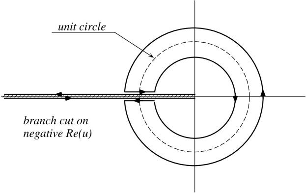
Figure 3: Contour on $u$-plane corresponding to $|\Psi^{(+)}(k,\varphi_{0})\rangle$. There appears a branch cut on the negative $\mathchoice{\hbox{\rm Re}}{\hbox{\rm Re}}{\hbox{\rm Re}}{\hbox{\rm Re}}(u)$ axis. If $\theta=0$, we cannot adopt the residue theorem because the pole is located just on the branch cut.

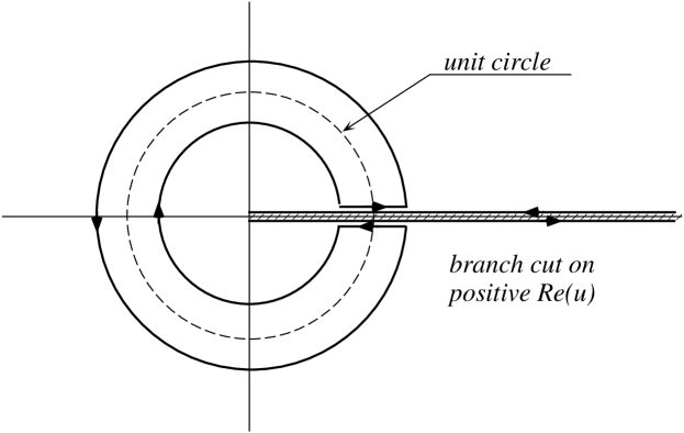
Figure 4: Another contour on $u$-plane corresponding to $|\Psi^{(-)}(k,\varphi_{0})\rangle$. The branch cut appears in the opposite (backward) direction for this case.

where the contours $C_{+}$ and $C_{-}$ are depicted in fig. 2. On change of variable $t\mapsto u=e^{t}$, there arises a multi-valued function $u^{-\alpha}$ in the integrand. Therefore we need to deal it with due care. If we recall that our solution for the scattering state, $|\Psi^{(+)}(k,\varphi_{0})\rangle$ in appendix B, has been obtained from the LS equation, we immediately notice that we have only one way to deform the contour to adopt the residue theorem to the integral on $u$-plane. (See fig. 3.) Another option for the deformation, fig. 4, obviously corresponds to another solution $|\Psi^{(-)}(k,\varphi_{0})\rangle$. As is seen from fig. 3, we can make use of the residue theorem to the contour integration around the unit circle only when $\theta\neq 0$. Then we obtain

$$\psi_{\alpha}=e^{ix\cos\theta-i\alpha(\theta-{\scriptstyle{\rm sgn}}({\theta})\pi)}-{\sin\pi\alpha\over\pi}\int_{-\infty}^{+\infty}dt{e^{(1-\alpha)t}\over{e^{t}-e^{i\theta}}}e^{ix\cosh t}\qquad(\theta\neq 0),$$ (C.5)

where

$$\mbox{\rm sgn}(\theta)=\left\{{\begin{array}[]{cc}1&(0<\theta\leq\pi)\\ -1&(-\pi\leq\theta<0)\end{array}}\right..$$ (C.6)

If we interpret the modulated plane wave $\psi_{\mathchoice{\hbox{\rm inc}}{\hbox{\rm inc}}{\hbox{\rm inc}}{\hbox{\rm inc}}}=e^{ix\cos\theta-i\alpha(\theta-{\scriptstyle{\rm sgn}}({\theta})\pi)}$ as an incident wave, the second term of (C.5) will be regarded as a scattered wave. Then we will obtain the Aharonov-Bohm scattering amplitude $f_{\mathchoice{\hbox{\rm AB}}{\hbox{\rm AB}}{\hbox{\rm AB}}{\hbox{\rm AB}}}(\theta)$ with the aid of the stationary phase approximation from

$$-{\sin\pi\alpha\over\pi}\int_{-\infty}^{+\infty}dt{e^{(1-\alpha)t}\over{e^{t}-e^{i\theta}}}e^{ix\cosh t}\sim{1\over\sqrt{r}}e^{ikr-i\pi/4}f_{\mathchoice{\hbox{\rm AB}}{\hbox{\rm AB}}{\hbox{\rm AB}}{\hbox{\rm AB}}}(\theta)\ .$$

So far the amplitude $f_{\mathchoice{\hbox{\rm AB}}{\hbox{\rm AB}}{\hbox{\rm AB}}{\hbox{\rm AB}}}(\theta)$ has not been treated in any connection with the $S$-matrix of the theory. Here it is important to note that we cannot define a $S$-matrix from (C.5) because $\psi_{\alpha}$ in (C.5) is not defined for $\theta=0$. Therefore it is inappropriate to decompose the total wave function in the form given above for considering the relation between the $S$-matrix and $f_{\mathchoice{\hbox{\rm AB}}{\hbox{\rm AB}}{\hbox{\rm AB}}{\hbox{\rm AB}}}(\theta)$. To find a definition of the $S$-matrix for this scattering problem, we need the asymptotic form of the total wave function

$$\psi_{\alpha}\sim\sqrt{2\pi\over x}\left[e^{-ix+i\pi/4}\delta(\theta+\pi)+e^{ix-i\pi/4}\left\{\cos\pi\alpha\delta(\theta)+\sqrt{k\over 2\pi}f_{\mathchoice{\hbox{\rm AB}}{\hbox{\rm AB}}{\hbox{\rm AB}}{\hbox{\rm AB}}}(\theta)\right\}\right]\ .$$ (C.7)

It should be then compared with (A.5) and with discussion below in appendix A. For the present case, the $S$-matrix should be defined by

$$\hat{S}=\cos\pi\alpha\leavevmode\mathchoice{\hbox{\rm tensysevensyfivesy\boldmath{$\displaystyle 1$}}}{\hbox{\rm tensysevensyfivesy\boldmath{$\textstyle 1$}}}{\hbox{\rm tensysevensyfivesy\boldmath{$\scriptstyle 1$}}}{\hbox{\rm tensysevensyfivesy\boldmath{$\scriptscriptstyle 1$}}}+\hat{f}_{\mathchoice{\hbox{\rm AB}}{\hbox{\rm AB}}{\hbox{\rm AB}}{\hbox{\rm AB}}}\ ,$$ (C.8)

which is nothing but the result given in (B.8). By equating both expressions in (C.8) and that in (B.9), we find

$$\hat{f}=(\cos\pi\alpha-1)\leavevmode\mathchoice{\hbox{\rm tensysevensyfivesy\boldmath{$\displaystyle 1$}}}{\hbox{\rm tensysevensyfivesy\boldmath{$\textstyle 1$}}}{\hbox{\rm tensysevensyfivesy\boldmath{$\scriptstyle 1$}}}{\hbox{\rm tensysevensyfivesy\boldmath{$\scriptscriptstyle 1$}}}+\hat{f}_{\mathchoice{\hbox{\rm AB}}{\hbox{\rm AB}}{\hbox{\rm AB}}{\hbox{\rm AB}}}\ ,$$ (C.9)

as the relation of the two scattering amplitudes. Therefore $\int_{-\pi}^{+\pi}d\theta|f_{\mathchoice{\hbox{\rm AB}}{\hbox{\rm AB}}{\hbox{\rm AB}}{\hbox{\rm AB}}}(\theta)|^{2}$ cannot be interpreted as the total cross section. As a consequence, $f_{\mathchoice{\hbox{\rm AB}}{\hbox{\rm AB}}{\hbox{\rm AB}}{\hbox{\rm AB}}}(\theta)$ does not obey the unitarity condition (A.7). Rather, it satisfies an operator relation

$$\hat{f}_{\mathchoice{\hbox{\rm AB}}{\hbox{\rm AB}}{\hbox{\rm AB}}{\hbox{\rm AB}}}^{\dagger}\hat{f}_{\mathchoice{\hbox{\rm AB}}{\hbox{\rm AB}}{\hbox{\rm AB}}{\hbox{\rm AB}}}=\sin^{2}\pi\alpha\leavevmode\mathchoice{\hbox{\rm tensysevensyfivesy\boldmath{$\displaystyle 1$}}}{\hbox{\rm tensysevensyfivesy\boldmath{$\textstyle 1$}}}{\hbox{\rm tensysevensyfivesy\boldmath{$\scriptstyle 1$}}}{\hbox{\rm tensysevensyfivesy\boldmath{$\scriptscriptstyle 1$}}}-\cos\pi\alpha(\hat{f}_{\mathchoice{\hbox{\rm AB}}{\hbox{\rm AB}}{\hbox{\rm AB}}{\hbox{\rm AB}}}^{\dagger}+\hat{f}_{\mathchoice{\hbox{\rm AB}}{\hbox{\rm AB}}{\hbox{\rm AB}}{\hbox{\rm AB}}})$$

because $S$-matrix itself has been shown to be unitary. In terms of the amplitude itself, it is expressed as

$$\int_{-\pi}^{\pi}d\varphi f_{\mathchoice{\hbox{\rm AB}}{\hbox{\rm AB}}{\hbox{\rm AB}}{\hbox{\rm AB}}}^{*}(\varphi-\varphi_{f})f_{\mathchoice{\hbox{\rm AB}}{\hbox{\rm AB}}{\hbox{\rm AB}}{\hbox{\rm AB}}}(\varphi-\varphi_{i})={2\pi\over k}\sin^{2}\pi\alpha\delta(\varphi_{f}-\varphi_{i})$$

because $f_{\mathchoice{\hbox{\rm AB}}{\hbox{\rm AB}}{\hbox{\rm AB}}{\hbox{\rm AB}}}(\theta)$ satisfies

$$f_{\mathchoice{\hbox{\rm AB}}{\hbox{\rm AB}}{\hbox{\rm AB}}{\hbox{\rm AB}}}^{*}(-\theta)+f_{\mathchoice{\hbox{\rm AB}}{\hbox{\rm AB}}{\hbox{\rm AB}}{\hbox{\rm AB}}}(\theta)=0\ .$$

Figure 1: Schläfli’s contour of integral representaion of $J_{\nu}(x)$. $C:\ -i\pi+\infty\rightarrow+i\pi+\infty$.

Figure 2: Contours $C_{+}$ and $C_{-}$. $C_{+}:\ -i\pi/2+\infty\rightarrow+i3\pi/2+\infty$, $C_{-}:\ i\pi/2-\infty\rightarrow-i3\pi/2-\infty$