Compactifications of F-Theory
on Calabi–Yau Threefolds – II

Abstract

We continue our study of compactifications of F-theory on Calabi–Yau threefolds. We gain more insight into F-theory duals of heterotic strings and provide a recipe for building F-theory duals for arbitrary heterotic compactifications on elliptically fibered manifolds. As a byproduct we find that string/string duality in six dimensions gets mapped to fiber/base exchange in F-theory. We also construct a number of new $N=1$, $d=6$ examples of F-theory vacua and study transitions among them. We find that some of these transition points correspond upon further compactification to 4 dimensions to transitions through analogues of Argyres–Douglas points of $N=2$ moduli. A key idea in these transitions is the notion of classifying $(0,4)$ fivebranes of heterotic strings.

1 Introduction

Compactifying F-theory on elliptic Calabi–Yau threefolds leads to theories in six dimensions with $N=1$ supersymmetry [1]. In this paper we continue our studies of such compactifications extending our previous results [2] by considering a more general class of Calabi–Yau threefolds.

The case considered in [2] was motivated by considering duals to perturbative heterotic string vacua compactified on $K3$. In particular for $E_{8}\times E_{8}$ compactifications we found that for instanton numbers $(12-n,12+n)$ for the $E_{8}$’s, the corresponding F-theory dual is compactification on the unique elliptic Calabi–Yau threefold with the base being the rational ruled surface ${\bf F}_{n}$. Moreover the $SO(32)$ heterotic string was conjectured to be dual to the $E_{8}\times E_{8}$ model with instanton numbers $(8,16)$.

In this paper we continue our studies in two directions: First of all we gain a better insight into the simple correspondence we found between instanton numbers and the degree of the rational ruled surface. In this way we find a recipe for how to build up F-theory duals to heterotic vacua in arbitrary dimensions compactified on elliptic manifolds with given bundle data. This investigation also leads us to reinterpret the F-theory/heterotic duality in 8 dimensions [1] as the statement of exchange symmetry between the fiber and the base of F-theory thus taking a step in geometrizing string/string duality.

We then consider other vacua of F-theory. Among these one can obtain all the non-perturbative heterotic vacua with fivebranes turned on [3, 4, 5] and some additional ones which do not have any heterotic analogue. Among these we find theories which have no tensor multiplets at all (which has also been noted in [5]). Also allowing for mild orbifold singularities in the base manifold we find that there are interesting classes of models which are stuck in phases with tensionless strings (and form an isolated class of $N=1$ vacua in $d=6$). In this way we find that the F-theory is a unifying setup for all the $N=1$ $d=6$ vacua.

We then talk about various types of transitions among these vacua. It has been suggested in [5, 6] that transitions among such vacua are through regions with tensionless strings. Since transitions among Calabi–Yau threefolds are well studied, and given that F-theory compactifications are on elliptic Calabi–Yau threefolds one can examine such transitions from the 4 dimensional viewpoint. In this way we find that upon compactifications to 4 dimensions the relevant six dimensional transitions get mapped to transitions of one of two types, one of which passes through an Argyres–Douglas point in the moduli of $N=2$ theories. Even though the physics of such transitions are not yet clear, the mathematical aspect of the extremal transition are fairly well understood. Moreover we find that at least a class of such transitions are related to exceptional groups $E_{n}$ (extending $n$ all the way down from 8 to 1). In particular we find a strong hint that in the heterotic theory there are different types of (0,4) 5-branes. Roughly speaking they should be in one to one correspondence with the degenerating types of $(0,4)$ conformal theories which are the perturbative heterotic vacua. We tentatively identify the $E_{n}$ type degeneration as the F-theory dual of heterotic string fivebranes corresponding to zero size instanton of gauge group $E_{n}$. We find examples of all such transitions. The most relevant one for the transition among $E_{8}\times E_{8}$ perturbative heterotic vacua are the $E_{8}$ type. Clearly there are other types of $(0,4)$ fivebranes and we believe we have taken a step in classifying them and their F-theory duals. We believe that further studies in extending this classification are very important.

The organization of this paper is as follows: In section 2 we review F-theory/heterotic duality in 8 dimensions. In section 3 we show how the $N=1$ F-theory/heterotic duality in 6 dimensions can be deduced from the 8-dimensional duality. In section 4 we make some general remarks about the spectrum of F-theory compactifications on Calabi–Yau threefolds. In section 5 we discuss the conditions imposed on the bases of the elliptic threefold by the condition of vanishing $c_{1}$ of the Calabi–Yau and find that in the case of the smooth bases they are all classified and are given by rational surfaces. In section 6 we give a number of examples. These include, apart from the ${\bf F}_{n}$ already discussed in section 3, ${\bf P}^{2}$ blown up at a number of points, Voisin–Borcea examples, as well as orbifold examples. Finally in section 7 we discuss singularities in the moduli space and transitions among the vacua.

2 F-Theory/Heterotic Duality in 8 Dimensions

In this section we recall the F-theory/heterotic duality in 8-dimensions [1]. We consider heterotic strings compactified to 8 dimensions on $T^{2}$. The moduli of this theory are characterized by specifying the complex structure $\tau$ and complexified Kähler structure $\rho$ of $T^{2}$ and in addition Wilson lines of $E_{8}\times E_{8}$ (or $SO(32)$) on $T^{2}$ characterized by 16 complex parameters. Altogether we thus have 18 complex parameters. They are given globally by the moduli space [7, 8]

$$SO(18,2;{\bf Z})\backslash SO(18,2)/SO(18)\times SO(2).$$ (2.1)

In addition there is a coupling constant of heterotic strings parametrized by a positive real number $\lambda^{2}\in{\bf R}^{+}$. The dual on the F-theory side is given by $K3$ compactifications which admit an elliptic fibration. The elliptic fiber, a torus, can be represented by

$$y^{2}=x^{3}+ax+b$$

which expresses it as a double cover of the complex plane $x$. The $K3$ surface can then be viewed as fiber space where the base is ${\bf P}^{1}$ and the fiber is the torus. Let us denote the coordinate of the ${\bf P}^{1}$ by $z$. Then the elliptic fibration is specified by

$$y^{2}=x^{3}+f(z)x+g(z)$$

where $f$ is of degree $\leq 8$ and $g$ is of degree $\leq 12$. Altogether we have 9+13 parameters specifying the polynomials $f$ and $g$, but we must mod out by the equivalence given by the $SL(2,{\bf C})$ action on ${\bf P}^{1}$ (3 parameters) and by one rescaling ($y\rightarrow\mu^{3}y,x\rightarrow\mu^{2}x,f\rightarrow\mu^{4}f,g\rightarrow\mu^{6}g$ for $\mu\in{\bf C}^{*}$), so that we end up with 18 complex parameters. It is well-known that this is also described by the above moduli space. Moreover there is an additional real parameter which is the size $A$ of ${\bf P}^{1}$ and we identify the heterotic coupling $\lambda^{2}$ with $A$.

There are generically 24 points on ${\bf P}^{1}$ where the elliptic fiber is degenerate. These 24 points are specified by the vanishing of the discriminant

$$\Delta=4f^{3}+27g^{2}.$$

The points where $\Delta=0$ can also be viewed from the type IIB viewpoint as the points where we have put 7-branes. This vacuum cannot be described in any perturbatively type IIB theory because the corresponding 7-branes belong to different $(p,q)$ strings [9, 10].

In order to get insight into this duality it is convenient to have a slightly more detailed relation between the parameters appearing in the function $f,g$ and the parameters in the heterotic vacuum. For the purposes of this paper it suffices to consider the following restricted class: Let us consider $E_{8}\times E_{8}$ heterotic strings compactified on $T^{2}$. Furthermore suppose we have no Wilson lines turned on and have an unbroken $E_{8}\times E_{8}$. Then the moduli of $T^{2}$ compactifications of the heterotic theory are given by the two complex parameters $(\tau,\rho)$ mentioned above. The F-theory dual is given by the two parameter family $(\alpha,\beta)$

$$y^{2}=x^{3}+\alpha z^{4}x+(z^{5}+\beta z^{6}+z^{7}).$$

To show that this is the right family it suffices to show that we do have $E_{8}\times E_{8}$ symmetry. Assuming that 7-branes with the ADE singularity give rise to the corresponding gauge group (a fact which can be checked perturbatively in type IIB only for the A-series) we should look for two points on ${\bf P}^{1}$ where the $K3$ acquires an $E_{8}$ singularities. In the above description the points $z=0$ and $z=\infty$ give rise to $E_{8}$ singularity. Let us show this first for the $z=0$ point. In that case the higher powers $\beta z^{6}+z^{7}$ in $g$ can be ignored. Moreover the term $xz^{4}$ is an irrelevant perturbation of the singularity $y^{2}=x^{3}+z^{5}$ (as it corresponds to a trivial element of the chiral algebra) so we have the familiar $E_{8}$ singularity (for a discussion in the context of Landau-Ginzburg theories see [11, 12]). As for the $z=\infty$ the same argument applies, when we note that in terms of $\tilde{z}=1/z$ and the appropriate rescaling of $x$ and $y$ the story is identical. In particular the $z^{7}$ term in the dual variable $\tilde{z}$ becomes $\tilde{z}^{5}$ (recalling that $g$ has degree $12$) and the first term still looks as $\tilde{z}^{4}x$ (as $f$ has degree $8$). Even though the precise map between $(\alpha,\beta)$ and $(\tau,\rho)$ can be worked out in terms of the j-functions we will only be interested in the regime of large $\alpha,\beta$ with $\alpha^{3}/\beta^{2}$ fixed. In this regime it is easy to read off that the elliptic fibration becomes essentially a constant as long as we keep away from 0 and $\infty$. On the heterotic side this limit will correspond to large $\rho$ and moreover the complex structure $\tau$ of the heterotic $T^{2}$ gets identified with the complex structure of the elliptic fiber of the F-theory! In this limit we will end up with a geometry of the 7-branes where in addition to the two $E_{8}$’s on the two sides of ${\bf P}^{1}$ we have two additional points where the elliptic fiber degenerates—one near $z=0$ and the other near $z=\infty$. Moreover this implies using the result of [13] that the geometry of the ${\bf P}^{1}$ becomes elongated looking like a sausage with the two tips of the sausage corresponding to $z=0$ and $z=\infty$ respectively. This follows from the fact that in this case we have divided the 24 7-branes into two groups of 12. Over most of the region where $z$ is not near $0$ or $\infty$ we simply have a cylinder over which we have a constant elliptic fiber. This ‘cylinder’ smells like a familiar story. It reminds one of how M-theory gives rise to $E_{8}\times E_{8}$ [14]. We will now argue why this may not be accidental and may be a geometric realization of string/string duality in the F-theory setup.

One may ask how the type I and heterotic strings can be realized in the F-theory set up. Given the M-theory description of them the idea is as follows (this has also been noted independently by [15]): Consider M-theory compactification on a cylinder down to 9 dimensions. This gives the heterotic/type I description in the M-theory setup [14]. Now if we take the limit where the volume of the cylinder shrinks to zero we get a type IIB description of the same object. This is clear when we also recall that the $\tau$ of type IIB arose from the M-theory side by compactifying on the two torus to 9 dimensions and taking the small volume limit of the torus [16, 9]. So we would say that F-theory on a cylinder gives $SO(32)$ type I/heterotic strings in 10 dimensions. Note that the fact that F-theory has no local on shell dynamics in the extra two dimensions make this a consistent picture [15], otherwise locality would have forced us to look for a product of two groups as the gauge group. At any rate the modulus of this cylinder is identified as the coupling constant of type I/heterotic strings. Note that this is also in accord with the fact that after orientifolding type IIB in 10 dimensions what is left of strong/weak self-duality of type IIB gets mapped to the strong/weak duality between type I and heterotic strings.

Thus we see that a description of heterotic strings compactified on $T^{2}$ down to 8 dimensions can also be viewed as the compactification of F-theory on a cylinder times $T^{2}$. On the other hand the F-theory/heterotic duality in 8 dimensions suggests that this is equivalent to the F-theory compactification on elliptic fibrations over ${\bf P}^{1}$ which in the above limit, apart from the tips of ${\bf P}^{1}$, becomes elliptic $T^{2}$ over the cylinder. Moreover the complex structure of the elliptic fiber $T^{2}$ is the same as the complex structure of the $T^{2}$ of the base on the heterotic side. The implication is clear: string/string duality seems to be the statement of the exchange symmetry between the base and the fiber in F-theory. We find this a very appealing picture of how string/string duality is geometrized in the F-theory set up.

One can also try to develop a similar picture in the M-theory setup. Of course by a further compactification on a circle the same picture repeats, namely, the duality between M-theory on $K3$ and heterotic strings on $T^{3}$ (which themselves can be viewed as M-theory on $T^{3}\times S^{1}/{\bf Z}_{2}$) can be seen as a geometric symmetry of M-theory when we combine one of the circles of $T^{3}$ with $S^{1}/{\bf Z}_{2}$ and form a cylinder and furthermore put the caps at the two ends to make it into a ${\bf P}^{1}$ as was the case above. It does however seem that there may also be a 9-dimensional version of the above story, when we think of defining the analogue of $K3$ in real algebraic geometry. Consider the real 2-manifold given by the solution to

$$y^{2}=x^{3}+f(z)x+g(z)$$

where $x,y,z$ are real and $f,g$ are real polynomials of degree 8 and 12 respectively. This can be viewed as a circle bundle (given by $(y,x)$) over $z$ and in a suitable limit does look like a cylinder. It is easy to see that now we have 18 real parameters to characterize this solution which could in principle be identified with the heterotic compactification on $S^{1}$ (including 16 Wilson lines, a radius and the coupling constant). Moreover we can consider a special limit in which $f=az^{4}$ and $g=z^{5}+bz^{6}+z^{7}$. In this case the two ‘ends’ of the universe are identified as $z=0,\infty$. It would be interesting to see if this picture can be identified directly with M-theory compactification to 9-dimensions on the above real surface.

3 $N=1$ F-Theory/Heterotic Duality in 6 Dimensions

In this section we will rederive some of the results in [2] in connection with F-theory duals of heterotic strings compactified on $K3$. We will heavily use the explicit map discussed in the previous section. The methods we will use can clearly be generalized to other compactifications (say to 4 dimensions). Our basic strategy is to use the above explicit map to piece together a certain amount of local data into a global picture. The data we need are of two types: One specifying the fact that we have $K3$ compactification of the heterotic strings and the other is the data about the bundle.

Let us recall the explicit parametrization we were considering in the previous section

$$y^{2}=x^{3}+\alpha z^{4}x+(z^{5}+\beta z^{6}+z^{7})$$

Recall from the previous section that in the large $\alpha$ and $\beta$ limit the complex structure of the torus $y^{2}=x^{3}+\alpha z^{4}x+\beta z^{6}$ is the same as that of the complex structure of the $T^{2}$ upon which the heterotic string is compactified. Given this map, the F-theory encoding of the $K3$ geometry of heterotic string compactification (or other elliptic compactifications) becomes straightforward. We view the $K3$ on the heterotic side as compactification of heterotic string on an elliptic fibration over ${\bf P}^{1}$ whose affine coordinate we denote by $z^{\prime}$. All we have to do is to require $\alpha$ and $\beta$ now be functions of $z^{\prime}$ of degree 8 and 12 respectively. We have thus taken care of the data needed to specify the $K3$ geometry of heterotic strings in the F-theory setup.

Now we come to the specification of the bundle data. We are considering $E_{8}\times E_{8}$ bundles. The simplest method to try begins by determining what a single instanton of zero size in an $E_{8}$ looks like. Suppose the instanton is localized at $z^{\prime}=0$. Then as long as we are away from this point we should have the $E_{8}$ gauge symmetry restored because after all an instanton of zero size is simply a singular gauge transformation with singularity at $z^{\prime}=0$. Let us concentrate on the first $E_{8}$ coming from the region near $z=0$. Away from $z^{\prime}=0$ the elliptic fibration data should be untouched, i.e., near $z=0$ but away from $z^{\prime}=0$ we should get

$$y^{2}=x^{3}+z^{5}$$

The most obvious way to modify this is to consider instead

$$y^{2}=x^{3}+z^{\prime}z^{5}$$

We conjecture that this is the analogue of a singular gauge transformation at $z^{\prime}=0$ in the singularity language. Note that away from $z^{\prime}=0$ we have the $E_{8}$ singularity as desired. One can immediately generalize this to having $k_{1}$ zero size instantons not necessarily all at the same point, where the locality of the above description implies we should have

$$y^{2}=x^{3}+g_{k_{1}}(z^{\prime})z^{5}$$

where $g_{k_{1}}$ is a polynomial of degree $k_{1}$. For the second $E_{8}$ coming from $z=\infty$ the same comments apply and so if we wish to have instanton number $k_{2}$ all of zero size at $z^{\prime}=0$ from the second one we should have for large $z$ the singularity which goes as

$$y^{2}=x^{3}+g_{k_{2}}(z^{\prime})z^{7}.$$

Now let us collect all these facts together and write the F-theory dual for a heterotic string which has $k_{1}$ zero size instantons for the first $E_{8}$ and $k_{2}$ for the second one on $K3$. To cancel heterotic anomalies (or more precisely if we wish to have no fivebranes [3]) we need to have $k_{1}+k_{2}=24$. It is convenient to write $k_{1,2}=12{\mp}n$. With no loss of generality we can take $0\leq n\leq 12$. From the above it is thus clear that the F-theory dual for this configuration is

$$y^{2}=x^{3}+f_{8}(z^{\prime})z^{4}x+g_{12-n}(z^{\prime})z^{5}+g_{12}(z^{\prime})z^{6}+g_{12+n}(z^{\prime})z^{7}$$ (3.1)

where the subscripts denote the degree of the polynomial. For this to make sense globally we must take $(z,z^{\prime})$ not to parameterize ${\bf P}^{1}\times{\bf P}^{1}$ but rather the rational ruled surface ${\bf F}_{n}$. In fact, if we introduce homogeneous partners $w$ and $w^{\prime}$ for $z$ and $z^{\prime}$ (and a pair of ${\bf C}^{*}$’s which act upon them, leaving the equation invariant), then in order to ensure that we have a family of $K3$ surfaces, $f(z,w,z^{\prime},w^{\prime})$ and $g(z,w,z^{\prime},w^{\prime})$ must be homogeneous of degrees 8 and 12 in $z$ and $w$. On the other hand, in order to ensure that we don’t get extra instantons at infinity, the polynomials $g_{k_{j}}(z^{\prime})$ must be extended to homogeneous polynomials in $z^{\prime}$ and $w^{\prime}$ of the same degree. Thus, the homogeneous form of (3.1) becomes

$$y^{2}=x^{3}+f_{8}(z^{\prime},w^{\prime})z^{4}w^{4}x+g_{12-n}(z^{\prime},w^{\prime})z^{5}w^{7}+g_{12}(z^{\prime},w^{\prime})z^{6}w^{6}+g_{12+n}(z^{\prime},w^{\prime})z^{7}w^{5}.$$ (3.2)

Taking the ratio of the last two terms in the equation, we find that the quantity $(z^{\prime})^{n}zw^{-1}$ must be invariant under the two ${\bf C}^{*}$’s. This means that the ${\bf C}^{*}$’s acting on $(z,w)$ and $(z^{\prime},w^{\prime})$ are not independent, and that we get ${\bf F}_{n}$ rather than ${\bf P}^{1}\times{\bf P}^{1}$ as the quotient.

Returning to the simpler “affine” form of the equation (3.1), we can now write the deformation away from zero size instanton to a finite size (as long as $n$ is not equal to 9,10,11 where $k_{1}=3,2,1$ zero size instantons cannot be made to ‘honest’ finite size instantons on $K3$) in the following form:

$$y^{2}=x^{3}+\sum_{k=-4}^{4}f_{8-nk}(z^{\prime})z^{4-k}x+\sum_{k=-6}^{6}g_{12-nk}(z^{\prime})z^{6-k}$$ (3.3)

where as usual the subscript denotes the degree of the polynomial with the condition that negative degree polynomials are set to zero.

These polynomials give the elliptic Calabi–Yau threefolds with base being ${\bf F}_{n}$ which were originally derived in [2]. There is one subtlety to note about this identification: the Weierstrass models we are using may have singularities. For example, if we find a subset of the space of polynomials appearing in (3.3) for which there are conifold singularities which admit a small resolution, then the moduli space of type IIA string theory compactified on Calabi–Yau threefolds will have an entire component corresponding to such polynomials. In F-theory, though, this should not be considered as a different model: the additional Kähler degrees of freedom provided by the small resolution are set to zero in F-theory, since they live within the fibers of the elliptic fibration. Thus, whereas the moduli space of the 4-dimensional theories may have several components, their F-theory limits form part of a space with only one component, completely determined by the base manifold $B$.

Before considering the various values of $n$ in the above duality, let us make a remark which will prove helpful in constructing more dual pairs in lower dimensions (and specifically for $N=1$ vacua in $d=4$). What we have learned is that if on the heterotic side we start with a compactification on an elliptically fibered manifold, the coefficients of $xz^{4}$ and $z^{6}$ specify all the geometry of the manifold. Moreover if we take the bundle data as $E_{8}\times E_{8}$ instantons of zero size, the sheaf theoretic bundle data can easily be translated to the geometry of the coefficients $z^{5}$ and $z^{7}$. Once we have constructed this singular limit of the duality we can extend it in principle in two directions: Either giving instantons finite sizes, or equivalently viewing the instantons of zero size as 5-branes, move them to other locations [17]. The above data is at the intersection of these two regions and serves as a bridge to either of the two types of vacua. The possibility of moving the 5-branes around has been considered in [5, 6] and we will consider it further in the F-theory setup in later sections after we discuss the duality with perturbative heterotic vacua on $K3$.

3.1 Determining the gauge group

Before discussing in detail the various possibilities for $n$, it will be useful to review how the singularities of the Weierstrass model (and hence nonabelian part of the gauge group) can be explicitly determined from a knowledge of the polynomials $f$ and $g$, where the equation has been written in Weierstrass form

$$y^{2}=x^{3}+f(z)x+g(z).$$

If we wish to determine the singularity type at the generic point of the $z=0$ locus in the base manifold, we should first calculate the discriminant

$$\Delta(z)=4f(z)^{3}+27g(z)^{2},$$

and then work out the orders of vanishing of $f(z)$, $g(z)$ and $\Delta(z)$ at $z=0$. Then according to Tate’s algorithm [18], the type of the fiber on Kodaira’s list and the singularity in the Weierstrass model are given as follows:

$\mathop{\rm ord}\nolimits(f)$	$\mathop{\rm ord}\nolimits(g)$	$\mathop{\rm ord}\nolimits(\Delta)$	fiber-type	singularity-type
$\geq 0$	$\geq 0$	$0$	smooth	none
$0$	$0$	$n$	$I_{n}$	$A_{n-1}$
$\geq 1$	$1$	$2$	$II$	none
$1$	$\geq 2$	$3$	$III$	$A_{1}$
$\geq 2$	$2$	$4$	$IV$	$A_{2}$
$2$	$\geq 3$	$n+6$	$I_{n}^{*}$	$D_{n+4}$
$\geq 2$	$3$	$n+6$	$I_{n}^{*}$	$D_{n+4}$
$\geq 3$	$4$	$8$	$IV^{*}$	$E_{6}$
$3$	$\geq 5$	$9$	$III^{*}$	$E_{7}$
$\geq 4$	$5$	$10$	$II^{*}$	$E_{8}$

If $\mathop{\rm ord}\nolimits(\Delta)>10$ then the singularity of the space is so bad that it destroys the triviality of the canonical bundle on a resolution.

We now turn to a consideration of the various values of $n$ in turn.

3.2 $n=0,1,2$

These cases were discussed in detail in [2]. In these cases it is easy to see that for generic polynomials $f$ and $g$, the elliptic curve (3.3) is generically non-singular. That the second $E_{8}$ coming from $z=\infty$ is generically completely Higgsed is true for all $n$ and this is perfectly consistent with the fact that the above elliptic curve is non-singular near $z=\infty$ (since all the relevant polynomials are non-vanishing for the highest powers in $z$, i.e., the $xz^{8}$ and $z^{12}$ terms). For the other $E_{8}$ coming from the $z=0$ region it is easy to see that for $n=0,1,2$ the singularity also disappears in this region. This is in accord with the fact that in these cases the gauge groups are completely Higgsed as can be seen from the heterotic side. The connection between $n=0$ and $n=2$ has been noted in detail in [2] where it is noted that they are in fact the same theory (similar remarks appear in [19]).

3.3 $n=3$

In all the cases $n>2$ the first $E_{8}$ cannot be completely Higgsed and we are left with some gauge group. In this case the most relevant terms near $z=0$ are $f_{2}$ and $g_{0}$ but since $xz^{2}$ is subleading to $z^{2}$ in the small $(x,z)$ region the singularity is that of

$$y^{2}=x^{3}+z^{2}$$

which is the $SU(3)$ singularity, so in this case we have a generic unbroken $SU(3)$ without matter (i.e., the singularity is of an ordinary type and the 7-brane analysis suffices to conclude we have no matter). This is in accord with the observation [3] that in this case there is a branch with a generic unbroken $SU(3)$.

3.4 $n=4$

This is a very interesting case, as it has been conjectured in [2] that not only does this correspond to $E_{8}\times E_{8}$ with instanton numbers $(8,16)$ but also to heterotic (or type I) $SO(32)$ string on $K3$ (see also [20]). One check for this is that both the $(8,16)$ $E_{8}\times E_{8}$ and $SO(32)$ heterotic strings leave an unbroken $SO(8)$ generically. This also follows from considering $SO(8)\times SO(16)$ bundles on $K3$ of instanton numbers $(8,16)$. This is a subbundle of both $SO(32)$ and $E_{8}\times E_{8}$ bundles of total instanton number 24 which resides as (8,16) in the $E_{8}\times E_{8}$ subgroup. Clearly this leaves an $SO(8)$ subgroup of the first $E_{8}$ unbroken. Moreover we expect no matter in this case. Now let us check whether the generic singularity of the F-theory dual is of this type. In this case the two lowest terms in (3.3) correspond to $f_{0}xz^{2}+g_{0}z^{3}$. Both of these terms are of the same order and the generic singularity can be written as

$$y^{2}=x^{3}+z^{3}\sim x^{3}+xz^{2}$$

and is recognized as that of $D_{4}$, i.e., $SO(8)$.

3.5 $n=5$

From the heterotic side we expect an $E_{6}$ generic singularity with a charged hypermultiplet in the $27$ (in addition to certain number of neutral hypermultiplets). In the F-theory description the leading term in (3.3) is $f_{3}(z^{\prime})xz^{3}+g_{2}(z^{\prime})z^{4}$ and thus the second term dominates and we have for the leading singularity

$$y^{2}=x^{3}+g_{2}(z^{\prime})z^{4}.$$

Note that generically this is the singularity for $E_{6}$ and so we should expect an $E_{6}$ gauge group. However the fact that we have at the zeros of $g_{2}(z^{\prime})$ a different singularity should be interpreted, in light of the above result in the heterotic string, as a signal of extra matter and in fact of a single 27 hypermultiplet.

3.6 $n=6$

This is similar to the case $n=5$ except that now on the heterotic side we expect to get $E_{6}$ with no extra matter and this is reflected by the fact that the leading singularity is now given by

$$y^{2}=x^{3}+z^{4}$$

which is the $E_{6}$ singularity without any extra singularities at special values of $z^{\prime}$.

3.7 $n=7$

In this case the leading terms in (3.3) come from $f_{1}(z^{\prime})xz^{3}+z^{5}g_{5}(z^{\prime})$ and the $xz^{3}$ term is more relevant than the $z^{5}$ term and so we get for the leading singularity

$$y^{2}=x^{3}+f_{1}(z^{\prime})xz^{3}$$

which is generically the $E_{7}$ singularity. Again since there is an extra singularity in the above when $f_{1}$ vanishes we expect extra charged matter. This is in accord with the heterotic string analysis where one ends up with $E_{7}$ gauge symmetry with a $1/2$ hypermultiplet of 56. Thus we learn through this example to recognize the above singularity as corresponding to an $E_{7}$ with half a 56 hypermultiplet. It would be interesting to verify this also from the analysis of monodromies and vanishing cycles as in [21].

3.8 $n=8$

This is very similar to the case above except that the relevant term is $f_{0}xz^{3}$ and so we end up with

$$y^{2}=x^{3}+xz^{3}$$

which is an ordinary $E_{7}$ singularity and we should have no extra charged matter. This is in accord with the heterotic string result.

3.9 $n=9,10,11$

In these cases the leading singularity is that of $E_{8}$ as the $z^{5}$ term is the more relevant term (except that in all cases we have extra singularities). On the heterotic side these correspond to zero size instantons which cannot be made to finite size ones, so the physics is somewhat singular. In fact these correspond to transition points noted above. Unlike the above cases where the extra singularity signaled the existence of extra matter, this does not seem to have a well defined meaning in this case as one sees from the heterotic side. These transitions will be discussed further below.

3.10 $n=12$

This is the case where the leading singularity is pure $E_{8}$ with no extra singularity. So we expect ordinary $E_{8}$. This is in accord with the fact that in this case all the instanton numbers are on the other $E_{8}$ bundle in the heterotic picture.

3.11 Matter from extra singularities

We have only explored a very tiny piece of information encoded in (3.3). For example, we can learn about how various extra singularities correspond to extra matter. We have seen some examples above and we can and should be more systematic. Just to give a flavor of what one means consider the cases above where we have the generic gauge group Higgsed to a subgroup of $E_{7}$. In this case by tuning appropriate moduli we can end up at special points where we have an extra $E_{7}$ singularity. For example tune the parameters so that the leading term comes from $f_{8-n}xz^{3}$, and thus the leading term is given by

$$y^{2}=x^{3}+f_{8-n}(z^{\prime})xz^{3}$$

From the heterotic side this corresponds to instanton number $12-n$ in the $E_{7}$ and we should expect to find ${1\over 2}k_{1}-2={1\over 2}(8-n)$ charged hypermultiplets in the 56 of $E_{7}$. This supports the above result that each time we see a zero in front of the $xz^{3}$ term this is a source of a half 56 of $E_{7}$ as was also found above. Had we tuned to obtain $E_{6}$ singularities instead we would have found

$$y^{2}=x^{3}+g_{12-2n}(z^{\prime})z^{4}.$$

From the heterotic side by further Higgsing the above $E_{7}$ to $E_{6}$ where we lose a 56 in the process of Higgsing and each surviving 56 turns into a pair of 27’s we learn that we would expect $k_{1}-6=6-n$ charged 27’s. This is again consistent with the fact that the coefficient of the above singularity is a polynomial of degree $2(6-n)$ in $z^{\prime}$ and suggests that each pair of zeroes in front of $z^{4}$ term gives rise to a $27$. Clearly by following various different branches of Higgsing we end up with various groups with varying amount of matter and we can thus begin to build up the dictionary of what matter representation corresponds to what kinds of singularity.

The geometric interpretation of this matter content should be this: along each curve $\Sigma_{i}$ in the base where the elliptic curves become singular, there is a generic singularity type but there are also finitely many points $P_{ij}$ where the singularity type changes. These may arise through intersections with other components $\Sigma_{k}$, or simply because of an extra vanishing of the polynomials $f$ and/or $g$ at those points. There is a vast array of possibilities for what kinds of singularities can arise; these have been classified mathematically [22, 23] under the assumption that the $\Sigma_{i}$’s meet transversally, but that might not always be the case. The simplest example of this phenomenon is the case of a curve of $A_{k}$ singularities meeting a curve of $A_{\ell}$ singularities, where a D-brane interpretation for the matter was given in [21].

4 General Remarks about F-Theory on Calabi–Yau 3-Folds

In this section we discuss some generalities about what spectrum to expect for F-theory compactifications on Calabi–Yau 3-folds. Consider an elliptic Calabi–Yau 3-fold $X$ with Hodge numbers $h^{1,1}(X)$ and $h^{2,1}(X)$. Note furthermore that we also have a base $B$ which has a certain Hodge number $h^{1,1}(B)$. Note that $h^{1,1}(B)+1$ and $h^{1,1}(X)$ need not be equal as there may be some Kähler deformations of the Calabi–Yau manifold which do not correspond to the Calabi–Yau being elliptically fibered.

We would like to determine how many tensor multiplets $T$, vector multiplets $V$ and hypermultiplets $H$ we have. The simplest thing to work out is the number of tensor multiplets $T$. The scalars in these multiplets are in one to one correspondence with the Kähler classes of $B$ except for the overall volume of $B$ which corresponds to a hypermultiplet [1]. We thus have

$$T=h^{1,1}(B)-1$$ (4.1)

In order to obtain further information about the rest of the degeneracies we use the fact that upon further compactification on $T^{2}$ our compactified F-theory model becomes equivalent to the type IIA theory compactified on the same Calabi–Yau [1]. We thus learn, by going to the Coulomb phase of the vector multiplets in the 4d sense, that

$$r(V)+T=h^{1,1}(X)-2$$ (4.2)

$$H^{0}=h^{2,1}(X)+1$$ (4.3)

where $r(V)$ denotes the rank of the vector multiplet and $H^{0}$ denotes the number of neutral hypermultiplets which are uncharged with respect to the Cartan of $V$. Combining the above with (4.1) we have

$$T=h^{1,1}(B)-1;\qquad r(V)=h^{1,1}(X)-h^{1,1}(B)-1;\qquad H^{0}=h^{2,1}(X)+1$$ (4.4)

We can determine the non-abelian factors in $V$ simply by studying the singularity type of the 7-branes (and if we had a better understanding of how various matter representations correspond to various type of singularities we could also have determined H in this way). We can thus deduce the number of $U(1)$’s because from (4.4) we know the total rank $r(V)$ of the gauge group.

On the other hand, for each non-abelian factor in $V$ the rank of that factor is one less than the number of components of the fiber lying over the corresponding curve in the base manifold. Geometrically, the elements of $H^{1,1}(X)$ must come from divisors in the base (i.e., $H^{1,1}(B)$), “extra” components of the reducible fibers (which contribute a total of $r(V^{\prime})$ to $h^{1,1}(X)$, where $V^{\prime}$ is the nonabelian part of the gauge group), and sections of the fibration. Comparing this with the spectrum of the F-theory, we see that the rank of the group of sections precisely gives the number of $U(1)$ factors in the gauge group. Roughly speaking what this means is that the number of $U(1)$’s is the number of ways we can choose the base manifold $B$ inside the elliptic Calabi–Yau.

The above constraints (together with the fact that the representations of non-abelian groups are typically rather constrained) are usually powerful enough to also fix $H$. There is a constraint from anomaly cancellation condition which requires that [24]

$$H-V=273-29T$$ (4.5)

where $H$ and $V$ denote the total number of hypermultiplets and vector multiplets respectively. This turns out to be a strong check on the spectrum of matter in the F-theory compactification discussed above.

5 The Structure of the Base

It is known [25, 26, 27] that for any elliptic fibration $\pi:X\to B$ of a Calabi–Yau threefold $X$, the base surface $B$ has at worst orbifold singularities. In fact, the singularities are more constrained than that: together with the collection of curves $\Sigma_{i}$ which specify where the elliptic fibration is singular, the singularities have a special property known as “log-terminal”. There are in fact not many surfaces which can occur as the base [26].

For our present purposes, we shall use the following properties of $B$. First of all, if the singularities of $B$ are resolved then $B$ is either a surface with $12K_{B}=0$ (i.e., a $K3$ surface, Enriques surface, hyperelliptic surface, or complex torus), or $B=(T^{2}\times{\bf P}^{1})/G$, or (the most common case) $B$ is a blowup of ${\bf P}^{2}$ or ${\bf F}_{n}$. In the case that $B$ is a $K3$ surface, a complex torus, a hyperelliptic surface, or $(T^{2}\times{\bf P}^{1})/G$, the corresponding Calabi–Yau will have a holomorphic one-form or a holomorphic two-form, and hence the corresponding type II compactification has extra supersymmetry. We shall exclude these cases from consideration.

Thus, for our purposes, we can take $B$ to be either an Enriques surface, a blowup of ${\bf P}^{2}$ or ${\bf F}_{n}$, or a surface with orbifold singularities whose resolution of singularities is one of the above.

6 Examples

In this section we discuss various examples of F-theory compactifications on Calabi–Yau threefolds. The first class of examples we consider correspond to the case where the base manifold is smooth, and should thus be, according to our previous discussion ${\bf P}^{2}$ or ${\bf F}_{n}$, blown up at various number of points. In the second class we find a large range of possibilities for the Hodge numbers. In the third class we explore the possibility of having orbifold singularities in the base. The fact that what we find seems self-consistent suggests that at least orbifold singularities of the base may be harmless for F-theory compactifications.

6.1 Blown up ${\bf F}_{n}$ as the base

Each of the ${\bf F}_{n}$ models reviewed in section 3 can be blown up to yield further models. We illustrate this by performing the blowup at $z=z^{\prime}=0$. The simplest way to do this is to introduce a new coordinate $u$, along with a ${\bf C}^{*}$ which acts on the coordinates as

$$(x,y,z,z^{\prime},u)\mapsto(\lambda^{2}x,\lambda^{3}y,\lambda z,\lambda z^{\prime},\lambda^{-1}u)$$

for $\lambda\in{\bf C}^{*}$, and to remove the locus where $z=z^{\prime}=0$ before forming the quotient by this action. When done in this way, the two coordinate charts which are usually used to describe a blowup are quite visible: when $z\neq 0$ we have

$$(x,y,z,z^{\prime},u)\sim(z^{-2}x,z^{-3}y,1,z^{-1}z^{\prime},zu)$$

and we should use those four quantities as coordinates; the other chart with $z^{\prime}\neq 0$ is obtained similarly.

However, in addition to a complex structure we should specify a value for the new Kähler class on the blowup. This is done by choosing a positive number $r$, and then describing the quotient by first imposing the constraint

$$\frac{1}{2}(2|x|^{2}+3|y|^{2}+|z|^{2}+|z^{\prime}|^{2}-|u|^{2})=r,$$

and then taking the quotient by $U(1)$ only. Notice that in this formulation, the removal of the locus $\{z=z^{\prime}=0\}$ is automatic.

To determine the equation for the Calabi–Yau threefolds in this space, we simply supplement each term in (3.3) with an appropriate power of $u$ in order to guarantee invariance under the new ${\bf C}^{*}$, obtaining:

$$y^{2}=x^{3}+\sum_{k=-4}^{4}\sum_{\ell=0}^{8-nk}f_{k\ell}\,z^{\prime}{}^{\ell}z^{4-k}u^{\ell-k}x+\sum_{k=-6}^{6}\sum_{\ell=0}^{12-nk}g_{k\ell}\,z^{\prime}{}^{\ell}z^{6-k}u^{\ell-k}.$$ (6.1)

Certain of the terms from the original equation—those with $\ell<k$ for $k\geq 0$—must be suppressed in the blown up model in order to obtain a Calabi–Yau hypersurface there. (That is, we must have $z^{\prime}{}^{k}|f_{8-nk}(z^{\prime})$ and $z^{\prime}{}^{k}|g_{12-nk}(z^{\prime})$ for $k\geq 0$.) So as expected, we find that $h^{1,1}$ increases and $h^{2,1}$ decreases during this type of blowup.

To generalize this construction somewhat, we can blow up a collection of points $z=0$, $z^{\prime}=a_{i}$, for $i=1,\dots,r$. If we let $\varphi(z^{\prime})=\prod(z^{\prime}-a_{i})$, then the condition on the equation becomes: $\varphi(z^{\prime})^{k}|f_{8-nk}$, $\varphi(z^{\prime})^{k}|g_{12-nk}$. This gets increasingly difficult to satisfy as $r$ increases. However, we can go as high as $r=24$ if we take $n=-12$ and choose our equation of the form

$$y^{2}=x^{3}+f_{8}(z^{\prime})z^{4}+\varphi(z^{\prime})z^{5}+g_{12}(z^{\prime})z^{6}+z^{7},$$

with unbroken $E_{8}\times E_{8}$. More generally, starting from any value of $n$ we can blow up as many as $12+n$ points along $z=0$ and $12-n$ points along $z=\infty$ by using a similar construction.

If we try to blow up points at arbitrary locations, however, it becomes increasingly difficult to verify that the terms suppressed in the newly blown up model do not cause unintended additional singularities in the space—singularities which could cause the Calabi–Yau condition to be violated. The blowing up of 24 points, which we were able to do when the points were in very special position, cannot be done if the points are generic.

So we will adopt a different strategy for producing examples: first we build models in which the base is already blown up a large amount, and then we study blow downs (by means of extremal transitions).

6.2 Blown up ${\bf P}^{2}$ as the base

If we blow up ${\bf P}^{2}$ at the 9 points of intersection of two cubic curves, we obtain a rational surface with an elliptic fibration (and a section). Generically there will be 12 singular fibers in such a fibration. Let $Y_{1}$ and $Y_{2}$ be two such blown-up ${\bf P}^{2}$’s. We can use the elliptic fibrations $\pi_{i}:Y_{i}\to{\bf P}^{1}$ to define a Calabi–Yau threefold, as follows:

$$X=\{(y_{1},y_{2})\in Y_{1}\times Y_{2}\ |\ \pi_{1}(y_{1})=\pi_{2}(y_{2})\}.$$

(This is called the “fiber product” construction, and was studied extensively in [28].) The threefold $X$ maps to $Y_{2}$ as a base manifold, and the fibers of that map are $T^{2}$’s whose complex structure is determined by the fibration $Y_{1}$.

The Hodge numbers are $h^{1,1}(X)=h^{2,1}(X)=19$, and all of the moduli can be obtained by varying the fibrations $Y_{1}$ and $Y_{2}$. This model was briefly discussed in [1], and has 9 tensor multiplets 8 vector multiplets and 20 hypermultiplets.

As shown in [28], and as we will see later, many more examples (with smaller values of $h^{1,1}$) can be produced from this one by extremal transitions.

6.3 The Voisin–Borcea examples

There is a rich class of elliptic Calabi–Yau threefolds studied independently by Voisin [29] and Borcea [30] and recently discussed by Aspinwall [31]. Start with a $K3$ surface $S$ which admits an involution $\sigma$ such that $\sigma^{*}(\omega)=-\omega$, where $\omega$ is the holomorphic $2$-form. Build a Calabi–Yau manifold of the form $S\times T^{2}/(\sigma,-1)$, resolving singularities appropriately. These are the Voisin–Borcea models. They are elliptically fibered over a base $B=S/\sigma$, and so can be used for F-theory compactification.

One way to produce such $S$’s and $\sigma$’s is to take one of the two ${\bf Z}_{2}$’s in our ${\bf Z}_{2}\times{\bf Z}_{2}$ orbifolding constructions, and mod out $T^{4}$ by it to produce a Kummer surface. But there are many more such pairs, all classified by Nikulin [32] in terms of three invariants $(r,a,\delta)$. These examples are plotted in figure 1 according to the values of $r$ and $a$; the open circles represent cases with $\delta=0$ (which means that the fixed locus of $\sigma$ defines a class in $H^{1,1}(S,{\bf Z})$ which is divisible by $2$) and the closed circles represent cases with $\delta=1$ (which means that the class of the fixed locus is not divisible by 2). In the case of invariants $(10,10,0)$, the surface $S/\sigma$ is an Enriques surface and the Hodge numbers of the corresponding threefold are $h^{1,1}=h^{2,1}=11$. In all other cases, $S/\sigma$ is a rational surface, and the Hodge numbers of the corresponding Calabi–Yau threefold are

$$h^{1,1}=5+3r-2a$$

$$h^{2,1}=65-3r-2a.$$

Figure 1: The Voisin–Borcea examples.

When $(r,a,\delta)=(10,10,0)$, $\sigma$ has no fixed points and $S/\sigma$ is an Enriques surface. When $(r,a,\delta)=(10,8,0)$, the fixed points of $\sigma$ consist of two curves of genus $1$. (In fact, in this case the Hodge numbers are (19,19) and we have the blown up ${\bf P}^{2}$ model discussed in the previous subsection.) In all other cases, the fixed points of $\sigma$ consist of a curve $C$ of genus $g$ together with $k$ rational curves $E_{1}$, …, $E_{k}$, where

$$g={1\over 2}(22-r-a)$$

$$k={1\over 2}(r-a).$$

The elliptic fibration over $B$ must have fibers of Kodaira type $I_{0}^{*}$ along each component of the fixed locus, and the Weierstrass model will have $D_{4}$ singularities over those components. To determine the structure of $B$, recall that the canonical bundle formula for an elliptic fibration then guarantees that

$$-K_{B}=\frac{1}{2}C+\sum_{i=1}^{k}\frac{1}{2}E_{i},$$

from which it follows that $c_{1}^{2}(B)=\frac{1}{4}(4g-4+(-4)k)=10-r$. Since $c_{1}^{2}(B)+c_{2}(B)=12$, we find that $c_{2}(B)=2+r$ and so $h^{1,1}(B)=r$. The number of tensor multiplets ranges from a low of 0 in the case $(r,a,\delta)=(1,1,1)$ (in which case $B={\bf P}^{2}$), to a high of 19 in the case $(r,a,\delta)=(20,2,1)$. Note that there are also several familiar models with exactly one tensor multiplet: $(2,0,0)$ which corresponds to ${\bf F}_{4}$, $(2,2,1)$ which corresponds to ${\bf F}_{1}$ and $(2,2,0)$ which corresponds to ${\bf F}_{0}$.

Let us verify the anomaly formula for these models (in the cases $(r,a,\delta)\neq(10,10,0),(10,8,0)$). There is an enhanced gauge symmetry of $SO(8)^{k+1}$, one factor of $SO(8)$ coming from each component of $-K_{B}$. On the other hand, from (4.4) we find

$$r(V)=(5+3r-2a)-r-1=4(k+1),$$

so there are no additional $U(1)$ factors in the gauge group. It follows that $V=28(k+1)$.

The factor of $SO(8)$ associated to $C$ has a matter representation consisting of $g$ adjoints, and so contributes $(28-4)g$ charged hypermultiplets to the spectrum. There is no matter coming from the other factors, since they are associated to rational curves. We therefore find that

$$H=(65-3r-2a)+1+24g,$$

and can verify the anomaly formula (4.5):

$$H-V=(65-3r-2a)+1+24(\frac{22-r-a}{2})-28(\frac{r-a}{2}+1)=273-29(r-1).$$

6.4 Orbifold examples

Some of the Voisin–Borcea examples have a simple orbifold description, which we will now discuss in more detail. Moreover we discuss also the Z-orbifold which is not among the Voisin–Borcea manifolds but presents a potentially interesting F-theory compactification.

If we consider an M-theory compactification on an elliptic orbifold and take the limit in which the Kähler class of the elliptic fiber goes to zero, we would expect to obtain in the limit the F-theory on the same orbifold. Thus we immediately are led to accept the existence of orbifold singularities in the base as harmless. In this section we consider 4 orbifold examples. Three of them correspond to ${\bf Z}_{2}\times{\bf Z}_{2}$ orbifolds and one corresponds to a ${\bf Z}_{3}$ orbifold giving rise to the Z-manifold.

Consider the Calabi–Yau threefold given by the orbifold of $T^{2}\times T^{2}\times T^{2}$. Let the coordinates of the tori be denoted by $z_{1},z_{2},z_{3}$. In the ${\bf Z}_{2}\times{\bf Z}_{2}$ examples we have the two generators flipping the sign of two out of three coordinates. Depending on whether they are accompanied by any extra shifts in the coordinates we end up with three possibilities. Let $g_{ij}$ denote the flipping of sign of $z_{i}$ and $z_{j}$. Then the three cases are:

(i) The two generators are $g_{12}$ accompanied by a shift of order 2 in $z_{3}$ and $g_{13}$ accompanied by a shift of order 2 in $z_{2}$. This manifold has Hodge numbers (11,11) (and has appeared in the context of type II/heterotic duality in [33]).

(ii) Same as above except $g_{13}$ is not accompanied by a shift. This manifold has Hodge numbers (19,19).

(iii) Same as above except with no shifts at all. This manifold has Hodge numbers $(h^{1,1},h^{12})=(51,3)$.

Except for the last case the other cases can be chosen to be F-theory vacua in two different ways depending on which $T^{2}$ we choose as the elliptic fiber. Here we consider the simplest possibility where the first $T^{2}$ is the elliptic fiber (the other cases have some interesting features which we have not fully understood).

In case (i) the base $B$ is the Enriques surface and has $h^{1,1}(B)=10$ so according to (4.4) we have $T=9$, $r(V)=0$, $H=12$. Note that the anomaly formula (4.5) is automatically satisfied. In this case the manifold can be deformed from the singular orbifold limit to a smooth manifold which still respects the elliptic fibration. This model is a Voisin–Borcea model with $(r,a,\delta)=(10,10,0)$.

In case (ii) the base manifold turns out to be the same as that studied in the previous section: ${\bf P}^{2}$ blown up at nine points. We thus have generically $U(1)^{8}$ and $T=9$, $H=12$. Again this manifold can be deformed away from the singular limit where the base is smooth. This model is dual to the models studied in the M-theory setup in [4] and as a type IIB orientifold in [34]. This is the same model as the Voisin–Borcea model with $(r,a,\delta)=(10,8,0)$.

Case (iii) is more interesting in that the gauge group is nonabelian even at generic values of the moduli. This model coincides with the Voisin–Borcea model with $(r,a,\delta)=(18,4,0)$, and we have verified the anomaly formula for it in the previous subsection.

Note that the divisor on the base manifold can be accounted for as $h^{1,1}(B)=16+1+1$, where 16 come from the fixed point of the group element $g_{23}$ and $1+1$ come from the Kähler classes of the second and third $T^{2}$. We thus find from (4.4) that $T=17$.

Finally we consider the case of the Z-orbifold which is given by modding $T^{2}\times T^{2}\times T^{2}$ with a ${\bf Z}_{3}$ which acts on each $T^{2}$ by $z\rightarrow{\rm exp}(2\pi i/3)z$ (and we are assuming that each $T^{2}$ does have the ${\bf Z}_{3}$ symmetry). The Kähler moduli of the base, compatible with elliptic fibration is 4 dimensional and we thus learn that $T=3$. Moreover since $(h^{1,1},h^{2,1})=(36,0)$ we learn from (4.4) that $r(V)=31$ and $H^{0}=1$. However the description of the low energy degrees of freedom are not just these. We will have tensionless strings, as we will discuss further in the next section. Note that this is the case where the physics is stuck at a place with tensionless strings where we cannot make a transition to other $N=1$ vacua and the vacuum appears to be isolated. This seems to indicate that $N=1$ vacua do not form a connected set in 6 dimensions. Note that the fact that the anomaly formula is not satisfied is another indication that we are missing certain states, and the local Lagrangian description does not suffice to describe this vacuum.

7 Transitions Among $N=1$ Vacua

We have constructed various examples of $N=1$ vacua in $d=6$ in the F-theory setup. It is natural to wonder whether there are transitions among them. Let us recall that in the F-theory setup the compactification is on an elliptically fibered Calabi–Yau threefold and that upon further compactification to 5 and 4 it is on the same moduli as M-theory and type IIA on the same manifold. If there is a transition among the vacua in 6-dimensions, there will clearly continue to be transitions upon further compactifications. This will give us a handle on various types of transitions as there are a number of tools available to study transitions among Calabi–Yau threefolds. However one has to be somewhat careful as the converse may not be true; in other words we may have transitions in 4d or 5d vacua which do not occur in 6d. One can also in principle imagine transitions among 4d vacua which do not give transitions in 5d, if one uses a finite value of the coupling constant of type IIA (which is related to the radius of the extra circle from 5 to 4) or the complexified Kähler class to make the transition.

Now suppose we start with type IIA compactification to four dimensions on a Calabi–Yau threefold which is elliptically fibered. If we consider a transition to another elliptically fibered Calabi–Yau and note that such a transition is insensitive to the size of the elliptic fiber or the coupling constant of type IIA, then in the limit of large coupling constant and zero size for the elliptic fiber we recover the F-theory transition in 6 dimensions. There are, however, transitions which connect elliptically fibered Calabi–Yau manifolds to non-elliptically fibered ones. These will not necessarily lead to transition in 6d. Thus even though the space of Calabi–Yau threefolds seems to be connected through extremal transitions, the same cannot be said about elliptically fibered ones, and in particular about the connectivity of $N=1$ vacua in 6d. An example of this is the Z-orbifold considered before which is not connected to any other Calabi–Yau unless we go through regions where the manifold is not elliptically fibered, i.e., we have to blow up the orbifold singularities which destroys elliptic fibration as we try to go to transition points to other Calabi–Yau manifolds. In the following we will divide our discussion into two parts, one involving the mathematical aspects of transitions, which is much better understood, and the other discussing the physical interpretation of such transitions.

7.1 Mathematical aspects of threefold transitions

The type IIA theory compactified on a Calabi–Yau threefold can undergo an extremal transition leading to another branch of the moduli space. We discuss these transitions from a mathematical perspective in this subsection.

In the semiclassical approximation, if we vary the Kähler moduli of a Calabi–Yau threefold $X$ so as to reach a boundary wall of the Kähler cone of $X$, some portion of $X$ shrinks to zero size. The precise ways in which this can happen are known from a mathematical analysis of the Kähler cone [35]: at a codimension one point of the boundary, we can either have

(i) the fibers of a $K3$ fibration or a $T^{4}$ fibration shrink to zero size, or

(ii) the fibers of an elliptic fibration shrink to zero size, or

(iii) a 2-cycle shrinks to a point, or

(iv) a 2-parameter family of 2-cycles shrink to points (i.e., a 4-cycle shrinks down to a 2-cycle), or

(v) a 4-cycle shrinks to a point.

Note that worldsheet corrections will affect the location of the singularity in the moduli space, but not its qualitative nature.

According to Hayakawa’s criterion [36], cases (i) and (ii) occur at points at infinite distance in the moduli space, while cases (iii), (iv) and (v) occur at finite distance. Case (iii) includes conifold points, where Strominger [37] showed how massless solitons cure the singularity in the physics (albeit from the mirror, IIB perspective). Case (iv) corresponds to enhanced nonabelian gauge symmetry [31, 21] where a similar analysis [38] shows how the physics gets corrected nonperturbatively. Case (v) is relatively unexplored, although examples have been discussed in [39].

In the conifold case [40] and in the enhanced gauge symmetry case [38], new branches of the moduli space can arise if the singularities have appropriate properties. Mathematically, at least, the same is true in case (v) in the examples discussed in [39].

The singularities which are introduced in case (v) when a 4-cycle shrinks to a point are of a special type known in the mathematics literature as “isolated canonical singularities with a crepant blowup”. A rough classification of these was given many years ago [41], based on the structure of the 4-cycles which occur. Such a 4-cycle must be a special type of complex algebraic surface known as a generalized del Pezzo surface; the adjective “generalized” refers to the fact that the surface itself can have singularities on it. We will primarily restrict our attention to the case in which this additional complication does not arise, and assume that the 4-cycle is actually a complex manifold.

Under this assumption, the del Pezzo surfaces are easy to classify: each such surface is either ${\bf P}^{1}\times{\bf P}^{1}$, or the blowup of ${\bf P}^{2}$ at $d$ general points, $0\leq d\leq 8$. If $S$ is such a surface, then $H^{1,1}(S)$ has rank $d+1$ (rank 2 in the case of ${\bf P}^{1}\times{\bf P}^{1}$), with generators consisting of a line from ${\bf P}^{2}$, and the exceptional divisors of the blowups (or the two ${\bf P}^{1}$’s in the case of ${\bf P}^{1}\times{\bf P}^{1}$). When $S$ appears on a Calabi–Yau threefold $X$, the image of the natural map $H^{1,1}(X)\to H^{1,1}(S)$ has some rank $k$ with $1\leq k\leq d+1$, which is an important invariant of the situation.

Each such surface $S$ on $X$ will lead to a potential extremal transition, provided that $S$ is contracted to a point when some wall of the Kähler cone is approached. The structure of this extremal transition appears to be this: the singular point can be smoothed through complex structure deformations to a new Calabi–Yau threefold $X^{\prime}$ leading to a new branch of the moduli space with Hodge numbers

$$h^{1,1}(X^{\prime})=h^{1,1}(X)-k$$

$$h^{2,1}(X^{\prime})=h^{2,1}(X)+c_{d}-k,$$

where $c_{d}$ is an invariant of the singularity type which we will discuss further below.

The surfaces $S$ possess some rather remarkable geometric structures [44, 45]. Assume for now that $d\geq 3$ and $S\neq{\bf P}^{1}\times{\bf P}^{1}$, and let $\ell$, $e_{1}$, …, $e_{d}$ denote the generators of $H^{1,1}(S)$. Then $c_{1}(S)=3\ell-\sum e_{i}$, and if we consider the lattice

$$\Lambda_{d}:=\{x\in H^{1,1}(S,{\bf Z})\ |\ x\cdot c_{1}(S)=0\},$$

then $\Lambda_{d}$ is naturally isomorphic to the root lattice of the root system $E_{d}$, with generators $\ell-e_{1}-e_{2}-e_{3}$, $e_{i}-e_{i+1}$. We thus get a natural action of the Weyl group $W(E_{d})$ on $H^{1,1}(S)$. One interesting feature of this Weyl group action is that it permutes the classes $\lambda\in H^{1,1}(S,{\bf Z})$ which satisfy $\lambda\cdot\lambda=-c_{1}(S)\cdot\lambda=-1$ (these can be thought of as the “lines” on $S$). The number of these “lines” is $6,10,16,27,56,240$ for $d=3,4,5,6,7,8$, respectively. The number $c_{d}$ which measures the change in Hodge numbers for $S$ embedded on a Calabi–Yau threefold is given by the dual Coxeter number of $E_{d}$.

The singularities which lead to these del Pezzo surfaces upon a crepant blowup can also be described quite explicitly [41] (at least for large values of $d$). They behave as follows:

(i) For $d=8$ the singularity is locally a hypersurface in ${\bf C}^{4}$ whose equation has leading terms $y^{2}=x^{3}+e_{2}(s,t)x^{2}+f_{4}(s,t)x+g_{6}(s,t)$, where $e$, $f$ and $g$ are homogeneous polynomials of the indicated degrees.

(ii) For $d=7$ the singularity is locally a hypersurface in ${\bf C}^{4}$ whose equation has leading terms $y^{2}=f_{4}(x,s,t)$ where $f_{4}$ is a homogeneous polynomial defining a nonsingular curve in ${\bf P}^{2}$.

(iii) For $d=6$ the singularity is locally a hypersurface in ${\bf C}^{4}$ whose equation has all of its leading terms of degree three, defining a nonsingular surface of degree 3 in ${\bf P}^{3}$.

(iv) For $d=5$ the singularity can be locally represented in ${\bf C}^{5}$ as the intersection of two hypersurfaces, both of whose leading terms are nondegenerate homogeneous quadratic polynomials.

(v) For $d\leq 4$, the singularity cannot be locally represented as a transverse intersection of hypersurfaces in some space.

7.2 Extremal transitions for elliptically fibered Calabi–Yau threefolds

We now consider which extremal transitions will occur for elliptically fibered Calabi–Yau threefolds. The Kähler parameters which we wish to vary in order to approach a transition point are the Kähler parameters coming from the base of the Calabi–Yau manifold. We wish to shrink some curve on the base to zero size, and then ask whether there is an extremal transition to another elliptically fibered Calabi–Yau threefold. In order for such a transition to exist, we must be able to smooth the base through complex deformations, in a way compatible with the existence of an elliptic fibration. The only curves on the base for which such a transition is possible are rational curves with self-intersection $-n$, for $n=1,2,4$. This is because the local functions $f$ and $g$ used in the Weierstrass equation must be sections of line bundles $-4K_{B}$ and $-6K_{B}$ on the singular base $B$ if the smoothing is to make sense, but in order for those multiples of $K_{B}$ to be line bundles, we must have $4(n-2)/n$ and $6(n-2)/n$ both being integers. This is only possible if $n$ divides $4$.

Note that in the case of elliptic Calabi–Yau manifolds over ${\bf F}_{n}$ the strong coupling transition point gets mapped to where a rational curve (denoted by $D_{v}$ in [2]) shrinks to zero size and that curve has self-intersection $-n$. The fact that for the cases of $1,4$ there could be transition has been anticipated in [5] based on anomaly considerations. It is satisfying to see that the mathematical conditions for transitions are captured by the anomaly considerations. The case $n=2$ is special and as has been argued in [2] it corresponds upon further compactification to 4 dimensions to $SU(2)$ gauge symmetry with an adjoint matter.

In order to determine the structure of these possible extremal transitions, we need to study an elliptic fibration defined on a neighborhood of a rational curve $C$ of self-intersection $-n$. In fact, this local study can be globalized, since we have available the surface ${\bf F}_{n}$ with elliptic fibrations over it which are sufficiently general to reproduce all possible local behaviors in a neighborhood of the curve of negative self-intersection. So we shall study the extremal transitions for those more global models, i.e., taking $C=D_{v}$ in the ${\bf F}_{n}$ model.

The $n=2$ case was studied in detail in [2]; let us review the main points. The curve $C$ satisfies $K_{B}\cdot C=0$, and so the locus where the fibers become singular does not meet $C$. It follows that the elliptic fibration over $C$ is a product $C\times T^{2}$ with a fixed complex structure on $T^{2}$. In particular, we can blow down $C\times T^{2}$ along the $C$ direction, leaving a curve of singularities of type $A_{1}$, and so (in the 4-dimensional theory) an $SU(2)$ enhanced gauge symmetry. The curve itself has genus one, so from the analysis of [46, 38] we expect a matter content of one adjoint hypermultiplet. At generic moduli the $SU(2)$ is broken, and the base surface must be deformed. In the global model over ${\bf F}_{2}$, this deformation corresponds to a “non-polynomial deformation” of the $WP_{1,1,2,8,12}^{4}$ model, in which the contracted ${\bf F}_{2}$ deforms to the smooth surface ${\bf F}_{0}={\bf P}^{1}\times{\bf P}^{1}$.

The $n=4$ case bears a number of similarities to the previous one. In order to satisfy the adjunction formula, $C$ must appear in the divisor for $-K_{B}$ with coefficient $1/2$. It follows that along the curve $C$, we must have an $SO(8)$ enhanced gauge symmetry. The Weierstrass fibration will have as its fiber a rational curve with a cusp, and the curve of cusps is a singular curve of the total space of type $D_{4}$. We can blow this down in the $C$ direction; the result will be a curve of $A_{1}$ singularities which is a rational curve with a cusp. There is a new $SU(2)$ gauge symmetry associated with this, in addition to the $SO(8)$ which is present for all values of moduli. At the cusp is hiding a rather complicated singularity, since the entire previous curve of $D_{4}$ singularities has mapped to this single point.

To see that the resulting space can be smoothed, we consider the global model. After contracting $C$ to a point, the base surface can be represented by $WP_{1,1,4}^{2}$ and the singular Calabi–Yau is a hypersurface in $WP_{1,1,4,12,18}^{4}$. There is a 2-1 cover of this base surface by $WP_{1,1,2}^{2}$, which is ${\bf F}_{2}$ with its $D_{v}$ contracted to a point. That is, we can realize $WP_{1,1,4}^{2}$ in the form $WP_{1,1,2}^{2}/{\bf Z}_{2}$. The fixed points of the ${\bf Z}_{2}$ consist of the singular point of $WP_{1,1,2}^{2}$, and another curve which does not pass through that point. The ${\bf Z}_{2}$-action can be lifted to the Weierstrass fibration, where it acts as $-1$ on the elliptic fibers. In terms of the homogeneous coordinates $[s,t,u,x,y,z]$ on $WP_{1,1,2,8,12}^{4}$, the ${\bf Z}_{2}$ acts as $-1$ on $u$ and $y$, and fixes the other variables. We can explicitly map the quotient to $WP_{1,1,4,12,18}^{4}$ by

$$[s,t,u,x,y]\mapsto[s,t,u^{2},u^{2}x,u^{3}y],$$

and note that a Calabi–Yau in the first space is mapped to a Calabi–Yau in the second. If we smooth $WP_{1,1,2}^{2}$ to ${\bf P}^{1}\times{\bf P}^{1}$, the ${\bf Z}_{2}$ action follows the smoothing and acts to swap the two ${\bf P}^{1}$ factors in ${\bf P}^{1}\times{\bf P}^{1}$. The quotient by that is ${\bf P}^{2}$; we see in this way that the ${\bf F}_{4}$ models with $D_{v}$ contracted smooth to the ${\bf P}^{2}$ model.

The extremal transition, blowing down to a curve of $A_{1}$’s with a cusp $P$, is illustrated in figure 2. This is similar to, but apparently different from, an extremal transition discussed by Aspinwall [31] in a similar context. Aspinwall was interested in preserving a K3 fibration, and so used a singular model of the elliptic fibration in which 4 disjoint surfaces over $C$ had been blown down to 4 curves of $A_{1}$ singularities (leading to a gauge symmetry enhancement of $SU(2)^{4}$) rather than the 4 surfaces we blow down in the Weierstrass model which lead to a single curve of $D_{4}$ singularities.

Figure 2: The extremal contraction with $n=4$.

We turn now to the extremal transitions in the case $n=1$. The elliptic fibration over $C$ defines a rational elliptic surface, generically with 12 singular fibers. We also have a distinguished section on that surface, the intersection of the global section of the Weierstrass fibration with the surface. Unlike the previous cases, this surface cannot be directly contracted to a curve, since the fiber type of the elliptic fibration varies. In order to learn how this transition works, we study the global model of the extremal transition from ${\bf F}_{1}$ to ${\bf P}^{2}$. Following the discussion in [2], the (3,243) Calabi–Yau threefolds with an elliptic fibration over ${\bf F}_{1}$ can be described as hypersurfaces in an ambient space determined by the following data: there is a space ${\bf C}^{7}$ with ‘homogeneous’ coordinates $s,t,u,v,x,y,z$ from which we remove the loci $\{s=t=0\}$, $\{u=v=0\}$, $\{x=y=z=0\}$ and then form quotient by the $({\bf C}^{*})^{3}$ action specified by the following table.

	$s$	$t$	$u$	$v$	$x$	$y$	$z$
$\lambda$	$1$	$1$	$1$	$0$	$6$	$9$	$0$
$\mu$	$0$	$0$	$1$	$1$	$4$	$6$	$0$
$\nu$	$0$	$0$	$0$	$0$	$2$	$3$	$1$

(The entries in the table denote exponents for the action of the ${\bf C}^{*}$’s on the homogeneous variables.) This ambient space is in fact a toric variety, and we can use the methods of toric geometry (see [47] for a review) to study the Kähler moduli. The columns in the table represent elements of $H^{1,1}$; in a more convenient basis, the action would be described by the following table.

	$s$	$t$	$u$	$v$	$x$	$y$	$z$
$\lambda\mu^{-1}\nu^{-1}$	$1$	$1$	$0$	$-1$	$0$	$0$	$-1$
$\mu\nu^{-2}$	$0$	$0$	$1$	$1$	$0$	$0$	$-2$
$\nu$	$0$	$0$	$0$	$0$	$2$	$3$	$1$

The columns of the matrix again represent generators of $H^{1,1}$; this basis has been chosen so that the Kähler cone is spanned by $(1,0,0)$, $(0,1,0)$ and $(0,0,1)$.

Our extremal transition should be described by shrinking the Kähler parameter corresponding to the curve of self-intersection $-1$ in the base, and this corresponds in the toric description to approaching the wall of the Kähler cone spanned by the second and third coordinates. When we approach that wall, however, we find that a 2-cycle shrinks to zero size rather than a 4-cycle. In fact, crossing that wall produces a “flop” of the Calabi–Yau space to another Calabi–Yau threefold, whose Kähler cone is spanned by $(0,1,0)$, $(0,0,1)$, and $(-1,1,1)$. (This flop is clearly signaled by the first row of our matrix of charges, which has as it’s nonzero entries $1$, $1$, $-1$ and $-1$.) After we make this flop, the resulting space maps to ${\bf P}^{2}$ rather than to ${\bf F}_{1}$, and the general fiber of the map is still a $T^{2}$, but the fiber over one point in ${\bf P}^{2}$ contains an entire 4-cycle. To complete the transition, then, we must also shrink this 4-cycle to zero size, and that is accomplished in the toric setup by proceeding to the wall of the new Kähler cone which is spanned by $(0,1,0)$ and $(-1,1,1)$. Along that wall, the 4-cycle has shrunk to zero size, and we can map the resulting threefold into ${\bf P}^{1,1,1,6,9}$ where its singularity can be smoothed by a complex structure deformation. Doing so goes to a different branch of the 4-dimensional moduli space.

It is worthwhile noting what lies on the other side of that second wall: we enter a somewhat non-geometric phase in the moduli space of the 4-dimensional theories, one in which one of the Kähler parameters has been replaced by some field localized at the singular point. The cone in $H^{1,1}$ associated with this new phase is spanned by $(0,1,0)$, $(-1,1,1)$ and $(-1,1,0)$. All three cones—which constitute a part of the enlarged Kähler moduli space for this—are illustrated in figure 3, with the F-theory boundary shaded.

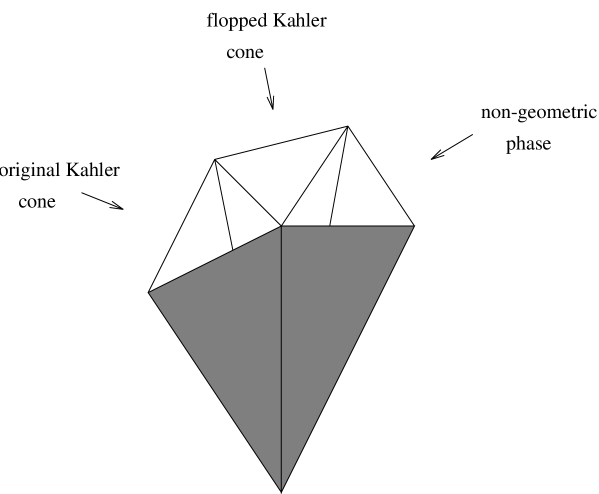
Figure 3: The F-theory moduli space on the boundary of the enlarged Kähler moduli space.

Note that in the limit where the fiber shrinks to zero (so that we get the F-theory moduli space) the second phase region lies on the boundary of the first. The third phase region shows up in the F-theory moduli space as the region where the area of $D_{v}$ has been formally extended to negative values, but as this is not a geometric region, it is not clear that there is actually an associated 6-dimensional theory.

We can describe this transition more abstractly as follows. Initially, lying over the curve of self-intersection $-1$ was a rational elliptic surface with a section, and such a surface must be the blowup of ${\bf P}^{2}$ in 9 points. In our transition, we first performed a flop on one of the ‘lines’ on this surface, leaving a divisor which is the blowup of ${\bf P}^{2}$ in 8 points, i.e., a del Pezzo surface with $d=8$. We then performed an extremal transition on that del Pezzo surface, leaving a singular point $P$. (This is illustrated in figure 4.) The structure of the transition is plainly visible in the behavior of the equations of the threefold during this process. The original equation took the form

$$y^{2}=x^{3}+\sum_{k=-4}^{4}xz^{4-k}f_{8-k}(z^{\prime})+\sum_{k=-6}^{6}z^{6-k}g_{12-k}(z^{\prime})$$

and has its terms constrained by the need to embed into the toric variety that fibers over ${\bf F}_{1}$. When we embed it into ${\bf P}^{1,1,1,6,9}$, however, we find that additional terms are permitted as new complex deformations:

$$\sum_{k=5}^{8}xf_{8-k}(z^{\prime})+\sum_{k=6}^{12}g_{12-k}(z^{\prime}).$$

In fact, if $z^{\prime\prime}$ is the third homogeneous coordinate on ${\bf P}^{2}$, we see that before adding in these new terms, there is a singularity at $z^{\prime}=z^{\prime\prime}=0$, where the leading terms are

$$y^{2}=x^{3}+xF_{4}(z^{\prime},z^{\prime\prime})+G_{6}(z^{\prime},z^{\prime\prime}),$$

where $F_{4}(z^{\prime},z^{\prime\prime})$ and $G_{6}(z^{\prime},z^{\prime\prime})$ are homogeneous polynomials in $z^{\prime}$ and $z^{\prime\prime}$. This is recognized immediately as the ‘canonical singularity with crepant blowup’ with $d=8$.

Figure 4: The flop and extremal contraction with $n=1$.

There is a natural generalization of this transition: instead of first flopping along a single section, we could flop along $k$ sections, leaving a del Pezzo surface with $d=9-k$. The extremal transition along that del Pezzo surface could then be done; as in the earlier case, the F-theory moduli space sees only the final result and not the intermediate steps. The new model produced in this way would have a larger number of sections of its elliptic fibration, and a smaller value of $h^{2,1}$.

7.3 Applications

We can now also discuss transitions among the elliptic Calabi–Yau manifolds over ${\bf F}_{n}$. The basic set up for this has been suggested in [5] based on M-theory considerations: We go to a region in hypermultiplet moduli where we get an $E_{8}$ instanton of zero size. This is the region where we can blow up and obtain one additional tensor multiplet whose scalar controls the value of the Kähler class of the blow up. The basic transition of this type is of the $E_{8}$ type corresponding to the $d=8$ transition discussed in detail above; in other words the basic setup of the transition is exactly the same one responsible for going from ${\bf F}_{1}$ to ${\bf P}^{2}$ (or backwards). This can be used to do two things: We can go from ${\bf F}_{n}$ to ${\bf F}_{n\pm 1}$ by blow ups and blow downs, or we can just blow up as many of the $E_{8}$ instantons as we please. Of course when we are left with less than instanton number 4 in either $E_{8}$ there will not exist any hypermultiplet moduli corresponding to giving a size to the instantons. In that case the instantons are necessarily all of zero size; this should be viewed as a boundary limit where all the instantons are blown up to tensor multiplets with the Kähler classes of some of the tensor multiplets tuned to correspond to zero size $E_{8}$ instantons. We will now discuss in detail how the ${\bf F}_{n}$ to ${\bf F}_{n\pm 1}$ transition works.

Recall that in (6.1) we blew up $z=z^{\prime}=0$ in ${\bf F}_{n}$ by introducing a new variable $u$ and a ${\bf C}^{*}$, and rewriting the equation as

$$y^{2}=x^{3}+\sum_{k=-4}^{4}\sum_{\ell=0}^{8-nk}f_{k\ell}\,z^{\prime}{}^{\ell}z^{4-k}u^{\ell-k}x+\sum_{k=-6}^{6}\sum_{\ell=0}^{12-nk}g_{k\ell}\,z^{\prime}{}^{\ell}z^{6-k}u^{\ell-k}.$$ (7.1)

To return to ${\bf F}_{n}$, we would simply set $u=1$; if instead we wish to map to ${\bf F}_{n+1}$ we can simply set $z^{\prime}=1$. This produces the equation for a Calabi–Yau fibering over that space.

In the process of doing this, we used one of the extremal transitions with $n=1$. After passing to ${\bf F}_{n+1}$, it may be possible to further deform the equation by adding new terms; this can affect the generic gauge symmetry of the model.

As another application, we can apply $n=1$ transitions to the $(19,19)$ model. We can blow down $(-1)$-curves successively until we get to the ${\bf P}^{2}$ model. At each stage, using the $d=8$ transitions, the Euler characteristic of the Calabi–Yau manifold changes by 60.

Finally, the transitions with $n=4$ can be used to relate the various Voisin–Borcea models. The rational curves occurring on those models when $k>0$ are curves of self-intersection $-4$, and if we make an extremal transition we alter the invariants as $k\mapsto k-1$, $g\mapsto g$, which is achieved via $(r,a)\mapsto(r-1,a+1)$. This links together large numbers of the transitions; further links can be made when $k=0$ by using the $n=1$ transitions.

7.4 Physical aspects of transitions

We would like to discuss some physical aspects of transitions and singularities encountered in the moduli space of the theory discussed in the mathematical setup in the previous section. The main case of interest is the singularities and potential transitions in the moduli space of tensor multiplets, which have a scalar. As discussed before the scalars in the tensor multiplets correspond to Kähler classes of the base manifold in the F-theory setup. Singularities are expected when the Kähler classes are tuned such that some 2-cycle in the base has vanishing area. For example, as noted in [2], in the case of F-duals of perturbative heterotic vacua one finds elliptic fibrations over ${\bf F}_{n}$. If $n\not=0$ it was shown in [2] that there is a 2-cycle, denoted by $D_{v}$ in [2] whose area goes as $k_{b}-{n\over 2}k_{f}$, where $k_{b,f}$ denote the Kähler classes of the base/fiber of ${\bf F}_{n}$. The scalar in the tensor multiplet controls $k_{b}/k_{f}$ and so when that reaches $n/2$ we have a vanishing 2-cycle. This in particular was the F-theory realization of the strong coupling puzzle raised in [3]. In particular the kinetic term of the gauge theory behaves as

$$\int(k_{b}-{n\over 2}k_{f})F^{2}$$

How do we understand this in the F-theory set up? This is essentially straightforward because the 2-cycle in question is part of the 7-brane world volume which is responsible for the gauge symmetry. In particular the 7-brane worldvolume is given by $D_{v}\times R^{6}$, thus the effective coupling constant for the gauge field in $R^{6}$ has a term proportional to the volume $D_{v}$ which thus explains the above singularity. The existence of this singularity is also marked by the existence of tensionless strings [5, 48]. From the viewpoint of a Lagrangian formulation these are simply the instantons of the gauge group which have zero action in the limit of infinitely strong coupling, thus leading to tensionless strings. From the viewpoint of F-theory these tensionless strings are the threebranes wrapped around the vanishing cycle $D_{v}$. Note that this is consistent with the instanton interpretation because a 3-brane wrapped partially around $D_{v}$ and living as a string in $R^{6}$ is itself inside a 7-brane and it is well known that one can view instantons living on D-branes as an equivalent description for the 4 lower dimensional D-branes sitting inside them [49, 50].

The main question is what happens after we hit such a wall where we have tensionless strings. In principle three things can happen: 1-Nothing, we are stuck at that point. 2- Continue formally to larger values of the Kähler parameter which formally would have yielded negative kinetic term for the gauge field. 3-Make a transition to a new branch of $N=1$ theories in 6 dimensions. For case (1) we have nothing to say and this case may in fact be the generic case. For case (2) we note that this is what one may expect in a lower dimensional theory such as compactifications down to 5 or 4 dimensions, for which the moduli of real Kähler moduli or complex Kähler moduli can be continued beyond the Kähler walls [47, 51]. However the question is whether they make sense in 6-dimensional terms. In the 4 or 5 dimensional cases typically the transition is to non-geometric phases, so it seems unlikely that in such regimes the 6 dimensional version can be defined. In particular, in general there may be no notion of taking the Kähler class of the elliptic fiber to be small. If the 4d transition is to phases which are geometric enough and moreover admit an elliptic fibration then one could in principle take the small Kähler class limit and recover a 6d transition. Otherwise it is difficult to justify the existence of 6-dimensional transitions.

As for point (3) above that is the most interesting aspect of these singularities. In the previous subsection we have given a mathematical analysis of the transition types available. In particular we found that there are only two basic types, corresponding to vanishing spheres with self-intersection $-n$ for $n=1,4$ (as discussed before the case $n=2$ does not lead to a transition). These two transitions were qualitatively very different because in the case of $n=4$ in 4 dimensions we get a curve of singularities on Calabi–Yau which signal an enhanced gauge symmetry point including an extra $SU(2)$ with possibly some matter content. In 4d terms this can in principle be some kind of Higgs mechanism, though it has to be studied further. In the $n=1$ case we have a very different type of transition which is bound to contain new physics as we will discuss now. Recall that the $n=1$ case has many subcases according to the geometry of the vanishing 4-cycle $S$ in the Calabi–Yau manifold. We discussed the classification of the simplest types of them in the previous section in terms of del Pezzo surfaces corresponding to $E_{d}$ groups. In the previous section we have used the $E_{8}$ type del Pezzo surface to go between various $F_{n}$’s. In fact it has been argued in [5, 6] that such transitions are also natural from the viewpoint of M-theory: In particular a 5-brane approaching the boundary of the 11-th dimension will give rise to a tensionless string (the membrane stretched from the 5-brane to the boundary). Moreover when it is at the boundary it can be viewed as an $E_{8}$ instanton of zero size. We can then give the instanton a finite size, thus making a transition to a model with one less tensor multiplet and (generically) 29 more hypermultiplets. Moreover it was noted in [5] that the same process can be described by blow up/down in the F-theory set up. Both the M-theory and the F-theory setup thus suggest that such transitions are natural. But unfortunately neither one really explains the physics of the transition. Let us try to develop the physics of transition as seen from the 4d perspective. In 4d the fact that a 4-manifold $S$ has shrunk to a point, means that we have the 2-cycles in $S$ shrinking as well as the 4-cycle $S$ itself shrunk to a point. It seems we have massless states corresponding to all the vanishing 2-cycles (which are realized as holomorphic curves) as well as the 4-cycle itself. Let $C$ be a 2-cycle realized by a holomorphic curve. Consider the intersection number $C\cdot S=C\cdot c_{1}(S)$, which is frequently non-zero. Intersecting vanishing 2- and 4-cycles signifies the appearance of massless electric and magnetic hypermultiplets. These are the analogues ( and perhaps extensions) of Argyres–Douglas [52] points of $N=2$ theories in string theory [53]. Let us assign magnetic $U(1)$ charge $1$ to the 4-cycle $S$. If $C\cdot S=k$ we then see that $C$ has electric charge $k$ under the same $U(1)$. Unfortunately we do not have a Lagrangian description of such points and thus the description of the transitions in this language is an interesting open problem. However there seem to be a number of additional hints which may shed light on the nature of the transitions we are encountering. As discussed above, among the states with $k=0$ (i.e., 2-cycles with $C\cdot S=0$) which are thus not charged under the $U(1)$, the root system of $E_{d}$ group naturally appears (as lines). Moreover if we consider a 2-cycle of fixed genus $g$ and electric charge (i.e., intersection number with $S$ equal to) $k$ under $U(1)$, the Weyl group of $E_{d}$ acts on them. Thus they can be taken to form a representation of $E_{d}\times U(1)$ (if we also include the zero-weight states), where the $E_{d}$ representation is fixed by the Weyl group action and the $U(1)$ charge is electric equal to $k$. For example as discussed in the previous section the $g=0,k=1$ case form well known representations of $E_{d}$ (the fundamental representation for $d=8,7,6$, the spinor for $d=5$ the anti-symmetric tensor representation for $d=4$ and $(3,2)$ representation for $E_{3}=SU(3)\times SU(2)$). These facts suggest that at these transition points we have an enhanced $E_{d}$ gauge symmetry together with some electric/magnetic quantum numbers of a $U(1)$. Note also that the representations are expected to grow larger as we consider arbitrary $g$ and $k$. We thus seem to get infinitely many massless modes which realize ever increasing representations of $E_{d}$. This sounds very similar to the story of how we get a huge number of higher genus 2-branes inside a $K3$ [54]. The story is similar here in that (ignoring the bundle choice of the cycle) the expected dimension of the family grows with genus (as $k+g-1$) and we thus expect a huge number of 2-brane states. However it is different in that here apparently all of them are becoming massless (as they are vanishing cycles) as we approach the transition point. Given the exponential growth expected in such states and the fact that we have a natural $E_{d}$ representation for all of them we conjecture that these states organize themselves into affine Kac–Moody algebras of the $E_{d}$ group (where the grading is related to $k,g$). We are currently investigating the validity of this conjecture. Note that this conjecture is also in line with the idea that the 6 dimensional version of the transition is through tensionless strings. Thus if the tensionless string carries an $E_{d}$ current algebra we would naturally get the above prediction where essentially the entire affine $E_{d}$ representation has seemingly collapsed to zero energy because the string has no tension.

Note that in the previous sections we showed how the $E_{8}$ case of these transitions allows one to go between ${\bf F}_{n}$’s and corresponds to points where an $E_{8}$ instanton has shrunk to zero size. In this sense one can expect that we should at least locally restore the $E_{8}$ symmetry that was broken by a finite size instanton. Here what we seem to be finding is that this seems to be the case with two subtleties that upon compactification to 4d we have not only infinitely many electric representations of the left-over $E_{8}$ but also some of them have relatively non-local charge with respect to the 4-cycle $S$. Similarly it is thus natural to conjecture that the other $E_{d}$ cases are also $F$-duals of $E_{d}$ instantons shrinking to zero size leaving us with a superconformal point of an $N=2$ theory with massless electric and magnetic states. It is important to study the physical meaning of transitions through such points. This is a case where at the present the mathematics of the transition is better understood than the physics of it. Hopefully we have provided some hints about the physics of it which will guide us in developing an effective physical formulation of transitions in $N=2$ superconformal field theories. Note that even though we may associate the $E_{d}$ cases with an instanton of $E_{d}$ of zero size, once we think of it as a heterotic fivebrane (corresponding to singularities of (0,4) superconformal theories) it has a life of its own and may appear in transitions where formally no gauge group exists. We have seen examples of this in the context of blow downs of the (19,19) model.

We would like to thank M. Bershadsky, B. Greene, M. Gross, A. Strominger and E. Witten for valuable discussions. D.R.M. would also like to thank the Harvard Physics Department for hospitality during the preparation of this paper. The research of D.R.M. is supported in part by NSF grant DMS-9401447, and that of C.V. is supported in part by NSF grant PHY-92-18167.

References

- [1] C. Vafa, hep-th/9602022.
- [2] D.R. Morrison and C. Vafa, hep-th/9602114.
- [3] M.J. Duff, R. Minasian and E. Witten, hep-th/9601036.
- [4] A. Sen, hep-th/9602010.
- [5] N. Seiberg and E. Witten, hep-th/9603003.
- [6] O.J. Ganor and A. Hanany, hep-th/9602120.
- [7] K. Narain, Phys. Lett. 169B (1986) 41.
- [8] K. Narain, M. Samadi and E. Witten, Nucl. Phys. B279 (1987) 369.
- [9] J. Schwarz, hep-th/9508143.
- [10] J. Schwarz, hep-th/9510086.
- [11] E. Martinec, Phys. Lett. B217 (1989) 431.
- [12] C. Vafa and N.P. Warner, Phys. Lett. B218 (1989) 51.
- [13] B.R. Greene, A. Shapere, C. Vafa and S.-T. Yau, Nucl. Phys. B337 (1990) 1.
- [14] P. Horava and E. Witten, hep-th/9510209.
- [15] P. Horava, private communication.
- [16] P.S. Aspinwall, hep-th/9508154.
- [17] E. Witten, hep-th/9602070.
- [18] J. Tate, in: Modular Functions of One Variable IV, Lecture Notes in Math. vol. 476, Springer-Verlag, Berlin (1975) 33.
- [19] G. Aldazabal, A. Font, L.E. Ibanez and F. Quevedo, hep-th/9602097.
- [20] E. Witten, hep-th/9603150.
- [21] M. Bershadsky, V. Sadov and C. Vafa, hep-th/9510225.
- [22] R. Miranda, in: The Birational Geometry of Degenerations, Progress in Math. vol. 29, Birkhäuser, 1983, 85.
- [23] A. Grassi, J. Algebraic Geom. 4 (1995), 255.
- [24] M.B. Green, J.H. Schwarz and P.C. West, Nucl. Phys. B254 (1985) 327; A. Sagnotti, Phys. Lett. B294 (1992) 196; J. Erler, J. Math. Phys., 35 (1994) 1819 ; J.H. Schwarz, hep-th/9512053.
- [25] A. Grassi, Math. Ann. 290 (1991), 287.
- [26] A. Grassi, Internat. J. Math. 4 (1993), 203.
- [27] K. Oguiso, Internat. J. Math. 4 (1993), 439.
- [28] C. Schoen, Math. Zeit. 197 (1988), 177.
- [29] C. Voisin, in: Journées de Géométrie Algébrique d’Orsay (Orsay, 1992), Astérisque No. 218 (1993), 273.
- [30] C. Borcea, “K3 surfaces with involution and mirror pairs of Calabi–Yau manifolds”, in: Essays on Mirror Manifolds vol. 2, in press.
- [31] P.S. Aspinwall, hep-th/9510142.
- [32] V. Nikulin, in: Proceedings of the International Congress of Mathematicians, Berkeley, 1986, 654.
- [33] S. Ferrara, J. Harvey, A. Strominger and C. Vafa, Phys. Lett. B361 (1995) 59.
- [34] A. Dabholkar and J. Park, hep-th/9602030.
- [35] P.M.H. Wilson, Invent. Math. 107 (1992), 561.
- [36] Y. Hayakawa, alg-geom/9507016.
- [37] A. Strominger, Nucl. Phys. B451 (1995) 96.
- [38] S. Katz, D.R. Morrison and M.R. Plesser, hep-th/9601108.
- [39] T.-M. Chiang, B.R. Greene, M. Gross and Y. Kanter, hep-th/9511204.
- [40] B.R. Greene, D.R. Morrison and A. Strominger, Nucl. Phys. B451 (1995) 109.
- [41] M. Reid, in: Journées de Géometrie Algébrique d’Angers, Juillet 1979, Sijthoff & Noordhoff (1980) 273.
- [42] Yo. Namikawa, “Stratified local moduli of Calabi–Yau 3-folds”, preprint, 1995.
- [43] M. Gross, alg-geom/9506022.
- [44] M. Demazure, in: Séminaire sur les Singularités des Surfaces, Lecture Notes in Math. vol. 777, Springer-Verlag, 1980, 23.
- [45] Yu.I. Manin, Cubic Forms, North-Holland, 1974.
- [46] A. Klemm and P. Mayr, hep-th/9601014.
- [47] P.S. Aspinwall, B.R. Greene and D.R. Morrison, Nucl. Phys. B416 (1994) 414.
- [48] M.J. Duff, H. Lü and C.N. Pope, hep-th/9603037.
- [49] M. Douglas, hep-th/9512077.
- [50] C. Vafa, hep-th/9512078.
- [51] E. Witten, Nucl. Phys. B403 (1993) 159.
- [52] P.C. Argyres and M. Douglas, Nucl. Phys. B448 (1995) 93.
- [53] E. Witten, hep-th/9507121.
- [54] M. Bershadsky, V. Sadov and C. Vafa, hep-th/9511222.
- [55] E. Looijenga, Invent. Math. 28 (1976) 17.
- [56] H. Pinkham, Proc. Symp. Pure Math. 30 (1977) 69.