CERN-TH/96-65

hep-th/9603074

Lectures on Superstring Phenomenology Fernando Quevedo Theory Division, CERN
CH-1211, Geneva 23
Switzerland

Abstract

The phenomenological aspects of string theory are briefly reviewed. Emphasis is given to the status of 4D string model building, effective Lagrangians, model independent results, supersymmetry breaking and duality symmetries.

Lectures Given at V Latin American Workshop on
Particles and Fields, Puebla, Mexico, November 1995

CERN-TH/96-65

March 1996

Introduction

We all know that quantum field theory (QFT) is the fundamental stone on which high energy physics is based [1]. This theory was developed in order to make consistent the general principles of special relativity and quantum mechanics, both fundamental to the study of elementary particles. Given the generality of QFT, there are very few general consequences we can extract from it. We can only mention: the existence of antiparticles, the running of coupling constants, the relation between spin and statistics and the CPT theorem.

To obtain more concrete information from QFT we need to consider specific models. For this we have a large degree of arbitrariness. We are free to choose the dimension of spacetime, the spin of the particles, the corresponding gauge group, of arbitrary rank, the number of different ‘matter’ fields of spin smaller than $1$ and their corresponding representation under the gauge group. Finally we are free to choose the couplings among those fields, renormalizable or not, including the potential for the scalar fields, gauge and Yukawa couplings, etc.

Given that degree of degeneracy, we need to use some experimental input in order to choose an appropriate QFT that could describe our world at least up to a given scale. Such a particular example is the current standard model of particle physics based on the gauge symmetry $SU(3)\otimes SU(2)\otimes U(1),$ with three families of quarks and leptons. This model describes fundamental physics up to a scale of $10^{2}$ GeV where $SU(2)\otimes U(1)$ is broken to electromagnetic $U(1)$. We want to emphasize that this is only one in an infinite number of QFTs and there is no reason other than experimental success to select this model.

Nevertheless, it is widely believed that the standard model is only an effective QFT that has to be generalized to a more fundamental theory. The main reasons for this belief are:

(i) Gravitation is not described at the quantum level. This is probably the most important problem of theoretical high energy physics.

(ii) The gauge hierarchy problem which, roughly speaking, refers to the fact that the $10^{2}$ GeV scale of symmmetry breaking is not stable under radiative corrections. In the presence of gravity it reduces to the question of why this scale is so small compared with the Planck scale of $10^{19}$ Gev.

(iii) There are also the ‘why’ problems (Why do we live in 4D?, Why is the gauge group $SU(3)\otimes SU(2)\otimes U(1)$?, Why are there three families?, Why do the couplings and masses of the matter fields take the particular values found by experiments? Why is the cosmological constant essentially zero? etc.).

Extensions of the standard model in terms of QFTs are many, and they partially address some of the problems mentioned above. For instance, supersymmetric field theories represent the best candidates to solve the hierarchy problem because the existence of a fermion-boson symmetry can stabilize the $10^{2}$ GeV scale[2]. There are also grand unified theories (GUTs), which unify the gauge couplings by imposing a simple gauge symmetry such as $SU(5)$, broken to the standard model at higher energies, and also the Kaluza-Klein theories where it is assumed that the world is actually higher-dimensional and the origin of gauge symmetries may be the extra small dimensions of spacetime. All of these extensions of the standard model are just different choices of QFTs and do not address the main problem of theoretical high energy physics, namely the quantization of gravity.

String theory is the only candidate for a fundamental theory of nature, encompassing all the known particles and interactions. In particular, it is the candidate theory for a consistent treatment of gravity in the quantum domain. String theory is not just another extension of the standard model in terms of a QFT, it is a generalization of the QFT itself. Roughly speaking the idea in string theory is to replace the point-like particles of QFT by one-dimensional extended objects, strings, which could be open or closed. Consistency requirements are very strict in string theory, selecting only five supersymmetric theories in 10D, namely: type I with gauge symmetry $SO(32)$, closed type II (A and B depending on orientation properties) and closed heterotic theories with gauge symmetries $SO(32)$ or $E_{8}\otimes E_{8}$. Similar to QFT, string theory has very few general ‘predictions’: There is an infinite tower of massive states corresponding to the oscillation modes of the string after quantization, the masses are quantized in terms of a fundamental scale which is identified with the Planck scale. On each of the five different theories there is always a massless particle of spin 2, the graviton $G_{MN}$, therefore strings imply the existence of gravity. Type I and heterotic have also massless particles of spin $1$, $A_{M}$, implying the existence of gauge symmetries and are therefore candidates to be ‘the fundamental theory of nature’. The spectrum also includes a singlet massless scalar, the dilaton $\Phi$ and antisymmetric tensors of different ranks depending on the string.

The effective theories describing the massless particles (the masses of observable particles are expected to arise from the ordinary Higgs effect at lower energies) are ordinary QFTs. We can see that string theories then lead to very restricted QFTs, with well defined symmetries and matter content. On the other hand each string theory has many (thousands or billions of) vacua. This allows us to construct string models in any number of dimensions less than $10$, including quasi-realistic models in 4D, which are very similar to the standard model, a very encouraging result. However, it also increases the level of arbitrariness, restricting the predictive power of the theory although, of course, the arbitrariness is still much less than in pure QFT’s.

The natural way to construct 4D string models is to start with a 10D theory and use the Kaluza-Klein idea of compactifying six dimensions in small spaces. Most of the variety of different vacua comes from the freedom to choose among these 6D spaces, then 4D string models are sometimes called superstring compactifications (SSC). We can also substitute the 6D space by some 2D conformal field theory (CFT) with specific properties as we will see in the next section.

4D string models are up to now the only candidates for a fundamental theory of nature. Their consistency also requires supersymmetry, which is a welcome property in view of the favourite solution to the hierarchy problem. Strings also improve the ‘why’ problem by changing many of them into a single dynamical question: Why do we live on this particular string vacuum or SSC? This situation is again much better than QFTs, but it is not completely satisfactory. We are left with at least two unsolved problems:

(i) How is supersymmetry broken, in order to recover the (non-supersymmetric) standard model at low energies?

(ii) How do we lift the vacuum degeneracy and select one single SSC describing our low energy world?

Fortunately, string theory is not yet completely understood, and this is not the final status of the theory. String theory is only understood at the perturbative level and non-perturbative questions, such as the tunnelling effect or possible comparison of different vacua, cannot be approached at the moment. A non-perturbative formulation of the theory is expected to give an answer to the why question above, it is also expected to provide the mechanism for the breakdown of supersymmetry at the electroweak scale, hopefully maintaining almost vanishing cosmological constant.

In these lectures I will review the field of string phenomenology. I will briefly mention the different attempts to construct a quasi-realistic 4D string model, including the obstacles that have been found so far to obtain a realistic model. Next I will discuss what is known about 4D effective actions including the tree-level Yukawa couplings as well as the one-loop corrections to the gauge couplings and nonrenormalization theorems. In chapter 4, I will present some vacuum independent general results of 4D strings. This is the closest we can get to real predictions of 4D string theories so far. Finally I will discuss briefly the problem of supersymmetry breaking and the possible use of duality symmetries in approaching this and other string problems.

Since this subject is so vast, I have to restrict to a very superficial discussion; general introductions to string theory and CFT can be found in [3]. There are also two collections of some of the more relevant papers on the subject of 4D strings. Ref. [4], includes the string model building techniques known before 1989, whereas ref.[5], contains some of the earlier phenomenological discussions of string theory. A number of review articles touching some of the topics of these lectures are provided in [6]

String Model Building

We mentioned in the introduction that there are only five consistent superstring theories in 10D. To build string models is the same as explicitly constructing the string vacua of each of these theories. By this we mean solutions of the corresponding background field equations of the different massless modes of the string.

Since there is no second quantized formulation of string theory, we need to use first quantization. In this case the basic quantity is the 2D worldsheet action, which for the bosonic string is:

$$S=\frac{1}{\alpha^{\prime}}\int d\sigma d\tau\left\{\left(G_{MN}(X)+B_{MN}(X)\right)\partial^{\mu}X^{M}\,\partial_{\mu}X^{N}+\alpha^{\prime}\Phi(X)\,^{(2)}R\right\}.$$ (1)

Let us describe the different quantities entering into this action. First the integral is over the 2D surface swept by the movement of the string. This surface is parametrized by $\sigma,\tau$. The inverse string tension $\alpha^{\prime}$ is the only (constant) free parameter of the theory. $X^{M}(\sigma,\tau),M=1,\cdots,D$ play two different roles: they are scalar fields in the 2D theory, but they are coordinates of the target space where the string propagates, which for critical string theories (the subject of this paper) has dimension $D=26$. Similarly $G_{MN}(X),B_{MN}(X),\Phi(X)$ are couplings of the 2D theory but since they are functions of $X$ they are fields in target space. $G_{MN}$ is a symmetric tensor which is identiified with the metric; $B_{MN}$ is an antisymmetric tensor field which in 4D target space will give rise to an axion field; and $\Phi$ is a scalar field, the dilaton. Since it appears only multiplying the 2D curvature ${}^{(2)}R$ whose integral is the topological invariant that counts the genus (number of holes) of the corresponding 2D surface, the vev of the dilaton is identified with the string coupling. These fields are always present in any closed string.

A fundamental symmetry of the above action is conformal invariance which includes scalings of the 2D metric as well as 2D reparametrization invariance. Imposing this symmetry at the 2D quantum level is similar to imposing that the coupling constants do not run in standard field theory. This then defines a 2D conformal field theory (CFT) and the constraints on the 2D couplings are the field equations for the target space fields $G_{MN},B_{MN},\Phi,A_{M}$. Not surprisingly the constraints give rise to Einstein’s equations, Yang-Mills equations and equations of motion for $B_{MN}$ and $\Phi$. To leading order in $\alpha^{\prime}$ these are the equations derived from the following target spacetime effective action:

$$S=\int d^{D}X\sqrt{G}e^{-\Phi}\left\{R-\frac{1}{12}\nabla_{M}B_{NP}\nabla^{M}B^{NP}+\nabla_{M}\Phi\nabla^{M}\Phi-\frac{D-26}{3}\right\}.$$ (2)

Since heterotic strings are supersymmetric, we have to add the corresponding fermionic partners of those fields. Solutions of these equations are then what we call string vacua and thus we can claim that there is a correspondence between string vacua and certain CFTs in 2D.

The simplest solution is of course 26D flat spacetime with constant values of all the fields. For this case we have a 2D free theory, which can be easily quantized by solving the wave equation $\partial^{\mu}\partial_{\mu}X^{M}=0$, the fields $X^{M}$ can be written as:

$$X^{M}(\sigma,\tau)=X_{R}^{M}(\tau-\sigma)+X_{L}^{M}(\tau+\sigma)$$ (3)

as usual, $X_{R}^{M}$ and $X_{L}^{M}$ represent right- and left-moving modes of the string respectively, with the mode expansion

$$X_{R}^{M}(\tau-\sigma)=x_{R}^{M}+p_{R}^{M}(\tau-\sigma)+\frac{i}{2}\sum_{n\neq 0}{\frac{1}{n}\alpha_{n}^{M}\,e^{-2in(\tau-\sigma)}}$$

$$X_{L}^{M}(\tau+\sigma)=x_{L}^{M}+p_{L}^{M}(\tau+\sigma)+\frac{i}{2}\sum_{n\neq 0}\frac{1}{n}\tilde{\alpha}_{n}^{M}\,e^{-2in(\tau+\sigma)}$$ (4)

Since this is a free theory, quantization assigns canonical commutation relations to the Fourier coefficients $\alpha_{m}^{N},\tilde{\alpha}_{m}^{N}$, like oscillators of the harmonic oscillator. The Hamiltonian then gives rise to the mass formula:

$$M^{2}=N_{R}+N_{L}-2.$$ (5)

Where $N_{R,L}$ refer to the harmonic oscillator occupation numbers for left and right movers and the level matching condition requires $N_{L}=N_{R}$ for consistency. Note that the ‘vacuum’ state ($N_{L}=N_{R}=0$) is a tachyon and the next state requires one left-moving and one right-moving oscillator ($N_{L}=N_{R}=1$), since both oscillators carry a target space index, the state corresponds to an arbitrary two-index tensor $\alpha_{-1}^{M}\tilde{\alpha}_{-1}^{N}|0\rangle$ of which the symmetric part is the metric $G_{MN}$, the antisymmetric part is $B_{MN}$ and the trace is the dilaton $\Phi$. That we can see are massless and are always present.

The instability due to the tachyon can be easily cured by supersymmetrizing the theory. In that case the tachyon state is projected out. The most popular supersymmetric string theory is the heterotic string. In this theory, only the right moving modes have a fermionic partner and consistency requires that they live in a 10D space rather than the 26D space of the bosonic string. The left moving modes however are purely bosonic, but the 26D space of these modes is such that the extra 16 coordinates are toroidally compactified, giving rise to extra massless states, which in this case are vector-like, as we will see next, and correspond to the gauge fields of $SO(32)$ or $E_{8}\otimes E_{8}$.

Toroidal Compactifications

In order to construct string models in less than 10D as well as to understand the heterotic string construction, we need to consider the simplest compactifications which correspond to the extra dimensions being circles and their higher dimensional generalization.

Let us first see the case of a circle. This means that the 10D space is represented by flat 9D spacetime times a circle $S^{1}$. We know that a circle is just the real line identifying all the numbers differing by $2\pi R$, where $R$ is the radius of the circle. So the only difference with the flat space discussed above are the boundary conditions. The solution of the wave equations are now as in (4). But now $p_{R}=m/2R-nR$ and $p_{L}=m/2R+nR$, $m$ is an integer reflecting the fact that the momentum in the compact direction has to be quantized in order to get single-valued wave function. The integer $n$ however refers to the fact that the string can wind around several times in the compact dimension and is thus named the ‘winding number’. The mass formula is then:

$$M^{2}=N_{R}+N_{L}-2+\frac{m^{2}}{4R^{2}}+n^{2}R^{2},\qquad N_{R}-N_{L}=mn.$$ (6)

This shows several interesting facts. First, for $n=0$ and varying $m$, we obtain an infinite tower of massive states with masses $\sim 1/R$; these are the standard ‘momentum states’ of Kaluza-Klein compactifications in field theory. In particular the massless states with $n=m=0$ and one oscillator in the compact direction are vector fields in the extra dimensions giving rise to a $U(1)_{L}\otimes U(1)_{R}$ Kaluza-Klein gauge symmetry. The states with $n\neq 0$ are the winding states and are purely stringy; they represent string states winding around the circle, they have mass $\sim R$. Second, there are special values of $m$ and $n$ which can give rise to extra massless states. In particular for $m=n=\pm 1$ we can see that at the special radius $R^{2}=1/2$ in units of $\alpha^{\prime}$, there are massless states with a single oscillator $N_{R}=1,N_{L}=0$ corresponding to massless vectors which in this case generate $SU(2)_{R}\otimes SU(2)_{L}$. This means that the special point in the ‘moduli space’ of the circle $R^{2}=1/2$ is a point of enhanced symmetry. The original $U(1)_{R}\otimes U(1)_{L}$ Kaluza-Klein symmetry of compactification on a circle gets enhanced to $SU(2)_{R}\otimes SU(2)_{L}$. This is a very stringy effect because it depends crucially on the existence of winding modes ($n\neq 0$). The third interesting fact about this compactification is that the spectrum is invariant under the following ‘duality’ transformations [7]:

$$R\leftrightarrow\frac{1}{2R}\qquad m\leftrightarrow n.$$ (7)

This is also a stringy property. It exchanges small with large distances but at the same time it exchanges momentum (Kaluza-Klein) states with winding states. This symmetry can be shown to hold not only for the spectrum but also for the interactions and therefore it is an exact symmetry of string perturbation theory.

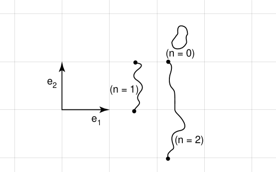
Figure 1: A 2D torus $T^{2}$ defined by the identification of points on ${\rm I\kern-1.79993ptR}^{2}$ by elements of the lattice defined by ${\bf e_{1}}$ and ${\bf e_{2}}$. We display examples of a closed string on ${\rm I\kern-1.79993ptR}^{2}$ which is also closed on $T^{2}$ ($n=0$), also a string closed on $T^{2}$ but not on ${\rm I\kern-1.79993ptR}^{2}$, winding around the torus once($n=1$) and twice ($n=2$).

Let us now extend the compactification to two dimensions, ie the 26D spacetime is the product of flat 24D spacetime and a 2D generalization of a circle, the torus $T^{2}$. Again the only difference with flat space is the boundary conditions. The two compact dimensions are identified by vectors of a 2D lattice, defining the torus $T^{2}$. Out of the three independent components of the compactified metric $G_{11},G_{22},G_{12}$ and the single component of $B_{MN}$ namely $B_{12}$ we can build two complex ‘moduli’ fields:

$$U\equiv\frac{G_{12}}{G_{22}}+i\,\frac{\sqrt{G}}{G_{22}}$$

$$T\equiv B_{12}+i\,\sqrt{G}.$$ (8)

$U$ is the standard modular parameter of any geometrical 2D torus and it is usually identified as the ‘complex structure’ modulus. $T$ is the ‘Kähler structure’ modulus (since $T^{2}$ is a complex Kähler space) and its imaginary part measures the overall size of the torus, since $\sqrt{G}$ is the determinant of the 2D metric. It plays the same role as $R$ did for the 1D circle. In terms of $T$ and $U$ we can write the left- and right-moving momenta as:

$$p_{L}^{2}=\frac{1}{2U_{2}T_{2}}\|(n_{1}-n_{2}\,U)-T\,(m_{2}+m_{1}\,U)\|^{2}$$

$$p_{R}^{2}=\frac{1}{2U_{2}T_{2}}\|(n_{1}-n_{2}\,U)-T^{*}(m_{2}+m_{1}\,U)\|^{2}$$ (9)

The mass formula, depending on $p_{L}^{2}+p_{R}^{2}$, again shows that there are enhanced symmetry points for special values of $T$ and $U$. It also shows the following symmetries:

$$U\rightarrow\frac{a\,U+b}{c\,U+d}\qquad T\rightarrow\frac{a\,T+b}{c\,T+d}\qquad T\leftrightarrow U.$$ (10)

Where $a,b,c,d$ are integers satisfying $ad-bc=1$. The first transformation is the standard $SL(2,{\bf Z})_{U}$ ‘modular’ symmetry of 2D tori and is independent of string theory; it is purely geometric. The second transformation is a stringy $SL(2,{\bf Z})_{T}$ named $T$-duality and it is a generalization of (7) for the 2D case. Again this is a symmetry as long as we also transform momenta $m_{1},m_{2}$ with winding $n_{1},n_{2}$. The third symmetry exchanges the complex structure $U$ with the Kähler structure $T$ and it is called ‘mirror symmetry’. If $U$ and $T$ each parametrize a complex plane $SL(2,{\rm I\kern-1.79993ptR})/O(2)$, the duality symmetry implies that they can only live in the fundamental domain defined by all the points of the product of complex spaces $SL(2,{\rm I\kern-1.79993ptR})/O(2)\otimes SL(2,{\rm I\kern-1.79993ptR})/O(2)\cong O(2,2,{\rm I\kern-1.79993ptR})/(O(2)\otimes O(2))$ identified under the duality group $SL(2,{\bf Z})_{U}\otimes SL(2,{\bf Z})_{T}=O(2,2,{\bf Z})$.

This is the situation that gets generalized to higher dimensions. In general, compactification on a $d$-dimensional torus has the moduli space ${\cal M}=O(d,d,{\rm I\kern-1.79993ptR})/O(d)\otimes O(d)$ with points identified under the duality group $O(d,d,{\bf Z})$. For the heterotic string with 16 extra left moving coordinates ${\cal M}=O(d+16,d,{\rm I\kern-1.79993ptR})/O(d+16)\otimes O(d)$ with a similar modification to the duality group. The left- and right- moving momenta $p_{L},p_{R}$ live on an even, selfdual lattice of signature $(22,6)$, which is usually called the Narain lattice $\Lambda_{22,6}$[8]. This generalizes the $\Lambda_{2,2}$ lattice defined by the integers $m_{1},m_{2};n_{1},n_{2}$ of eq. (9).

We can easily verify in this case that the dimension of ${\cal M}$ is $d(d+16)$ corresponding to the number of independent components of $G_{mn},B_{mn},A_{m}^{I}$ with $m,n=1\cdots d;I=1,\cdots 16$. For $d=6$ we have a 4D string model with a moduli space of dimension $132$. To this we have to add the dilaton field $\Phi$ which, together with the spacetime components of the antisymmetric tensor $B_{\mu\nu}$, can be combined into a new modular parameter:

$$S\equiv a+i\,e^{\Phi}.$$ (11)

Here the axion field $a$ is defined as $\nabla_{\mu}a=\epsilon_{\mu\nu\rho\sigma}\nabla^{\nu}B^{\rho\sigma}$. $S$ parametrizes again a coset $SL(2,{\rm I\kern-1.79993ptR})/O(2)$. It is then natural to believe there is also a duality symmetry for the field $S$ of the type $SL(2,{\bf Z})$; by analogy with the situation for $T$ and $U$. Such a symmetry was proposed in ref.[9] and it has received a lot of attention recently. If true it may have far reaching consequences since (similar to equation (7)) it relates strong to weak string coupling.

Orbifold Compactifications

We have then succeeded in constructing 4D superstring models from toroidal compactifications and understand the full class of these models given by the moduli space ${\cal M}$. Unfortunately, all of these models have $N=4$ supersymmetry and therefore they are not interesting for phenomenology, because they are not chiral. To obtain a chiral model we should construct models with at most $N=1$ supersymmetry. If we still want to use the benefits of free 2D theories, we should construct models from flat space and modify only the boundary conditions. We have already considered identifications by shift symmetries of a lattice defining the tori. We still have the option to also use rotations and consider ‘twisted’ boundary conditions [10]. As an example let us start with the torus $T^{2}$ discussed before. If we make the identification $X^{i}\rightarrow-X^{i}$ we are constructing the orbifold $O^{2}\equiv T^{2}/{\bf Z}_{2}$, shown in figure 2, where the ${\bf Z}_{2}$ twist is rotation by $\pi$. This space is not a manifold because it is singular at the points left fixed by the rotation $\{(0,0),(0,1/2),(1/2,0),(1/2,1/2)\}$. Notice that, for instance, the point $(1/2,1/2)$ is fixed because it is transformed to $(-1/2,-1/2)$ which is identical to the original point after a lattice shift. In general, the discrete group of rotations defining the orbifold is called the point group ${\cal P}$, whereas the nonabelian group including the rotations and also the translations of the lattice $\Lambda$, is the space group ${\cal S}$. So usually a torus is defined as $T^{d}\equiv{\rm I\kern-1.79993ptR}^{d}/\Lambda$ and an orbifold $O^{d}\equiv T^{d}/{\cal P}\equiv{\rm I\kern-1.79993ptR}^{d}/{\cal S}$.

Figure 2: Starting from the two-torus $T^{2}$, we generate the orbifold $O^{2}\equiv T^{2}/{\bf Z}^{2}$, ‘the ravioli’, by the identification $\vec{x}\leftrightarrow-\vec{x}$. $O^{2}$ is singular at the four ‘fixed points’ shown. Besides the momentum and winding states of the torus, the orbifold spectrum also has ‘twisted’ states, corresponding to strings closed in $O^{2}$ but not on $T^{2}$. The twisted states are attached to fixed points, we display one example.

We can easily construct 4D strings from orbifold compactifications in which the 10D spacetime of the heterotic string is the product of 4D flat spacetime and a six-dimensional orbifold $O^{6}$. The heterotic string is particularly interesting because we can extend the action of the point group to the 16D lattice of the gauge group by embedding the action of the orbifold twist in the gauge degrees of freedom defined by the $E_{8}\otimes E_{8}$ lattice, say. This can easily be done in two ways:

(i) Perform a homomorphism of the point group action in the gauge lattice by shifting the lattice vectors by a vector $V=ML$ where $M$ is the order of the point group and $L$ is any lattice vector in 16D.

(ii) Perform the homomorphism by twisting also the gauge lattice by an order $M$ rotation belonging to the Weyl group of the corresponding gauge group.

These embeddings on the gauge degrees of freedom allow us to break the gauge group, reduce the number of supersymmetries and generate $N=1$ chiral models in 4D as desired. The reason for this is the following: using the embedding by a shift $V$, we start with the spectrum of the toroidal compactification and have to project out all the states that are not invariant by the orbifold twist. For the gauge group, only the elements satisfying $P\cdot V\in{\bf Z}$ remain, where $P\in E_{8}\otimes E_{8}$, breaking the gauge group to a subgroup of the same rank. The four gravitinos of the $N=4$ toroidal compactification also transform and depending on the orbifold twist they are reduced to only one or two invariant states, indicating that there is only $N=2$ or $N=1$ supersymmetry. Actually there are only four twists ${\bf Z}_{M}$ leading to $N=2$ (for $M=2,3,4,6$) and some twenty ${\bf Z}_{M}$ or ${\bf Z}_{M}\otimes{\bf Z}_{N}$ twists leading to $N=1$ supersymmetry [11], which are the phenomenologically interesting ones. For each of these twists we can have several ($\sim 10$) different embeddings on the gauge degrees of freedom. One of these embeddings is called the standard embedding because it acts identically in the gauge degrees of freedom as in the 6D space, this embedding also describes compactifications of the type II strings and is distinguished because in the 2D worldsheet, the corresponding model has two supersymmetries on the left-movers and two supersymmetries on the right-movers, the corresponding models are called $(2,2)$ models. All other embeddings do not have supersymmetry in the left moving side and are called $(0,2)$ models.

On top of all these embeddings we can also add Wilson lines [12] $A_{m},m=1,\cdots,6$, by embedding the shifts of the lattice defining the 6D compactified torus, on the gauge degrees of freedom in terms of further shifts of the 16D gauge lattice, which will further break the gauge group. This increases the number of possible consistent models by a large amount, which we can only estimate between millions and billions because some may turn out to be actually equivalent. The Wilson lines can also be interpreted as the full embedding of the space group ${\cal S}$ in the gauge degrees of freedom. In this case, using the two alternative embeddings mentioned above will give a completely different result because in the first case, both $V$ and the Wilson lines $A_{i}$ will act as shifts and so the embedding is abelian, whereas in the second option we will have both shifts and twists so the embedding is non-abelian. This possibility allows for two important properties: the Wilson lines are continuous rather than quantized and the rank of the gauge group can be reduced. In the absence of Wilson lines both embeddings are equivalent. Both classes of embeddings can be obtained by starting with the Narain lattice of toroidal compactifications $\Lambda_{22,6}$ and twist it in a consistent manner. This already takes into account the discrete and continuous Wilson lines (which were already present, parametrizing $\Lambda_{22,6}$) and also allows for the possibility of performing left-right asymmetric twists, the so-called asymmetric orbifolds [13]. This extra degree of freedom increases the number of possible models.

We can see now how a vast amount of heterotic string orbifold models can be generated. There are many (billions?) classes of models; different classes differentiated by the choice of original 6D toroidal lattice, the orbifold point group, the embeddings $V$ and the discrete Wilson lines. But each of these discrete choices allows for a variation of different continuous parameters such as the moduli fields (like $S,T,U$), the continuous Wilson lines (that correspond to charged untwisted sector moduli fields) and there are also charged twisted-sector moduli fields[14]. All the continuous parameters can be seen as flat potentials for fields in the effective field theoretical effective action.

Only a few of these classes of models includes quasi-realistic models. As an example [15], the model based on the ${\bf Z}_{3}$ orbifold with embedding $V$ and nonvanishing Wilson lines $A_{m}$ given by:

$$V=\frac{1}{3}\left(1,1,1,1,2,0,0,0\right)\otimes\left(2,0,\cdots,0\right)$$

$$A_{1}=A_{2}=\frac{1}{3}\left(0,0,\cdots,2\right)\otimes\left(0,1,1,0\cdots,0\right)$$

$$A_{3}=A_{4}=\frac{1}{3}\left(1,1,1,2,1,0,1,1\right)\otimes\left(1,1,\cdots,0\right)$$ (12)

breaks $E_{8}\otimes E_{8}$ to $SU(3)\otimes SU(2)\otimes U(1)\otimes U(1)^{7}\otimes SO(10)$ with three families of quarks and leptons. The extra $U(1)^{7}$ symmetry can be broken by the standard Higgs mechanism which, in string theory requires the existence of flat directions among some charged matter fields; these can be analyzed in the models at hand because there are general ‘selection rules’ forbidding couplings not invariant under the action of the point and space groups. The $SO(10)$ remains as a hidden sector (in the sense that it only has gravitational strength couplings with the observable $SU(3)\otimes SU(2)\otimes U(1)$ sector). This is an example of a quasi realistic model. The structure of Yukawa couplings can be analyzed leading to very realistic properties and problems such as very fast proton decay can be avoided. However, there are extra doublets in the model that give rise to unrealistic values of Weinberg’s angle. This may in principle be solved by contemplating the existence of intermediate scales, but at this point the model stops being stringy. It also has the drawback that without knowing details about supersymmetry breaking many of the low energy parameters can not be determined. There are variations of this model that allow for an extra $U(1)$ symmetry at low energies, implying a relatively light $Z^{\prime}$ particle. There are several models in the literature with similar properties as this one, showing that it is possible to get models very close to the standard model of particle physics. But there is not a single model that could be considered realistic. In particular there is no model yet with just the spectrum of the supersymmetric standard model.

Calabi-Yau compactifications

We saw that the orbifolds obtained from twisting the 6D tori can give rise to chiral $N=1$ models in 4D. Orbifolds are singular objects but they can be smoothed out by blowing-up the singularities at the fixed points. The resulting smooth manifold is a so-called Calabi-Yau manifold [16]. Mathematically, these are 6D complex manifolds with $SU(3)$ holonomy or equivalently vanishing first Chern class. They were actually the first standard Kaluza-Klein compactification considered in string theory, leading to chiral 4D models and generically gauge group $E_{6}\otimes E_{8}$, with $E_{8}$ a hidden gauge group.

The drawback of compactifications on Calabi Yau manifolds is that they are highly nontrivial spaces and we cannot describe the strings on such manifolds, contrary to what we did in the case of free theories such as tori and orbifolds. In particular we can not compute explicitly the couplings in the effective theory, except for the simplest renormalizable Yukawa couplings.

On the other hand, Calabi-Yau manifolds have been understood much better during the past few years and have lead to some beautiful and impressive results. In a way they are more general than orbiifolds because an orbifold is only a particular singular limit of a Calabi-Yau manifold. Also there are other constructions of these manifolds which are not related to orbifolds. They can be defined as hypersurfaces in complex (weighted) projective spaces ${\rm I\kern-1.79993ptP}^{4}_{(k_{0},k_{1},k_{2},k_{3},k_{4})}$ where $k_{i}$’s are the weights of the corresponding coordinates for which there is the identification $z_{i}\cong\lambda^{k_{i}}z_{i}$. The hypersurface is defined as the vanishing locus of a polynomial of the corresponding coordinates. For instance the surface defined as:

$$P\equiv z_{1}^{12}+z_{2}^{12}+z_{3}^{6}+z_{4}^{6}+z_{5}^{2}=0$$ (13)

defines a Calabi-Yau manifold with weights:$(1,1,2,2,6)$. The relation $\sum_{i}k_{i}=d$ where $d$ is the degree of the polynomial ensures that the surface is a Calabi-Yau manifold. The manifold is guaranteed to be smooth if both the polynomial $P$ and its derivatives do not vanish simultaneously. Larger classes of manifolds can be constructed by considering intersections of hypersurfaces in higher dimensional projective spaces, the so-called complete intersection Calabi-Yau manifolds (CICY). Actually, it is known in the mathematical literature, that all Calabi-Yau spaces can be defined as (intersection of) hypersurfaces in weighted projective spaces. Large numbers of these manifolds have been classified, although the full classification is not complete. The mathematical estimate is that there are of the order of ten thousand Calabi-Yau manifolds. The corresponding string models are of the type $(2,2)$. Some of the highlights of Calabi-Yau compactifications are the following:

(i) There are classes of moduli fields, generalizing the fields $T$ and $U$ of the two-torus mentioned before. The number of these fields is given by topological numbers known as Hodge numbers $h_{i,j},i+j\leq 3$. They correspond to the number of complex harmonic forms that can be defined in the manifold with $i$ holomorphic indices and $j$ antiholomorphic indices. Then the number of complex structure fields (U) is given by $h_{2,1}$ and the number of Kähler structure fields ($T$) is given by $h_{1,1}$. Many of the $h_{2,1}$ forms correspond to the coefficients of different monomials which can be added to the defining polynomial that still give rise to the same space, other forms correspond to the blowing up of possible singularities. Many of the $h_{2,1}$ forms correspond to polynomial deformations of the defining surface, but others are related with the reparation of singularities. For Calabi-Yau manifolds we have $h_{1,1}\geq 1$, therefore there is always a special Kähler class deformation which can be thought as the overall size of the corresponding manifold, it is usually called, the Kähler form. All the other Hodge numbers of Calabi-Yau manifolds are fixed ($h_{3,0}=h_{0,3}=1,h_{1,0}=h_{0,1}=0,h_{0,2}=h_{2,0}=0$)

(ii) The gauge group in 4D is $E_{6}\otimes E_{8}$. The matter fields transform as ${27}$’s or ${\overline{2}7}$’s of $E_{6}$. The number of each is also given by the Hodge numbers $h_{1,1},h_{1,2}$ and the number of generations is then topological:$N_{g}\equiv h_{1,1}-h_{1,2}=\chi/2$ where $\chi$ is the Euler number of the manifold. This is one of the most appealing properties of these compactifications since they imply that topology determines the number of quarks and leptons.

(iii)Mirror symmetry [17]. Similar to the 2D toroidal compactifications, it has been found that there is a mirror symmetry in Calabi-Yau spaces that exchanges the moduli fields $T_{m}$ and $U_{a}$ $m=1,\cdots h_{1,1}$, $a=1,\cdots,h_{2,1}$. This means that for every Calabi-Yau manifold ${\cal M}$, there exists another manifold ${\cal W}$ which has the complex and Kähler structure fields exchanged, ie $(h_{1,1},h_{2,1})\leftrightarrow(h_{2,1},h_{1,1})$ and opposite Euler number $\chi$. The mirror symmetry of the two-torus described previously, is only a special example on which the manifold is its own mirror. Mirror symmetry is not only a nontrivial contribution of string theory to modern mathematics, but it has very interesting applications for computing effective Lagrangians as we will see in the next chapter. it also relates the geometrical modular symmetries associated to the $U_{a}$ fields of the manifold ${\cal M}$ to generalized, stringy, $T$-duality symmetries for the mirror ${\cal W}$ and viceversa (see for instance [18] ).

(iv) Even though these string models are not completely understood in terms of 2D CFTs, special points in the moduli space of a given Calabi-Yau are CFTs, such as the orbifold compactifications mentioned before. In fact some people believe that there is a one to one correspondence between string models with $(2,2)$ supersymmetry in the worldsheet and Calabi-Yau manifolds. There is also a description of CFTs in terms of effective Landau-Ginzburg Lagrangians which are intimately related to Calabi-Yau compactifications as two phases of the same 2D theory [19]. In particular the potential of that Landau-Ginzburg theory is determined by the polynomial $P$ defining the Calabi-Yau hypersurface.

(v) There are also few models with three generations that, after the $E_{6}$ symmetry breaking, could lead to quasi-realistic 4D strings. One of these models was analyzed in some detail [20]. Usually, $E_{6}$ models also lead to the existence of extra $Z^{\prime}$ particles of different kinds. They have been thoroughly studied because of the potential experimental importance of detecting an extra massive gauge boson (for a recent discussion see ref. [21] ).

(vi) Although most of the Calabi-Yau models studied so far correspond to standard embedding in the gauge degrees of freedom ($(2,2)$ models), there is also the possibility of constructing $(0,2)$ models by performing different embeddings, similar to the orbifold case. This increases substantially the number of string models of this construction [22].

Other Constructions

During the past few years several other constructions of chiral 4D strings in four dimensions, have been found in terms of explicit CFT’s. We described before how the use of free field CFT’s lead us naturally to orbifold compactifications. We can also use the property of these 2D field theries for which there is an equivalence between fermions and bosons. Since the bosonic fields in 2D are the coordinates in target space, by fermionizing them we lose the geometrical interpretation, but it is a consistent string model as long as we keep the 4D spacetime coordinates as bosons. If we fermionize all the extra coordinates and choose nontrivial boundary conditions on the fermions we can get nontrivial 4D strings [23], which do not have to have a geometrical interpretation in terms of compactifications!. Many models have been studied using this approach which, in many cases, are equivalent to orbifold compactifications at some particular value of the radius. Some quasi-realistic models have been studied with much detail using this approach. This includes models with three families and standard model gauge group $SU(3)\otimes SU(2)\otimes U(1)$ as well as a version of $SU(5)\otimes U(1)$ known as flipped $SU(5)$ [24]. In some cases again, the models reproduce many of the nice features of the standard model. Nevertheless, as in the case of orbifolds, there is not a totally realistic model yet.

A related approach uses bosonization in the opposite direction ie it bosonizes all of the fermions of the (supersymmetric) right moving sector (including the ghost system needed for consistent quantization of the 2D theory) [25]. This is the so called covariant lattice approach which in some way generalizes the Narain lattice of toroidal compactifications. Again many of these models are equivalent to orbifolds at a particular radius. In particular some of the three generation orbifold models mentioned before have been explicitly reproduced using this approach [27].

A probably more general construction goes into the name of Gepner-Kazama-Suzuki models [26]. They depart from free field CFTs and construct more general CFTs by using cosets $G/H$ to describe the CFT of the ‘internal’ dimensions. This construction includes (products of) statistical mechanics models such as the Ising and Potts models and their supersymmetric generalizations. One of the salient features of these constructions is that for the models with $(2,2)$ supersymmetry in the worldsheet, it can be shown explicitly that they do correspond to particular points of Calabi-Yau compactifications, despite of their original non-geometric construction. This was found by using their realization in terms of Landau-Ginzburg 2D effective field theories. Generalization of these constructions to $(0,2)$ supersymmetric models have also been achieved and a large class of models exist [28], including some close to the standard model.

We have then seen that there are several formalisms for constructing chiral 4D strings. Many models can be built using different approaches. Each formalism has advantages and disadvantages in terms of the level of generality and for performing explicit calculations for the low energy effective theory.

Effective Actions in 4D

We have seen that consistent 4D chiral string models lead to $N=1$ supersymmetry. For phenomenological purposes, we are interested in finding the effective action for the light degrees of freedom, that means we want to integrate out all the heavy degrees of freedom at the Planck scale $M_{p}$ and compute the effective couplings among the light states (massless at the Planck scale). This will be a standard field theoretical action with $N=1$ supersymmetry. The on-shell massless spectrum of these models have the graviton-gravitino multiplet $(G_{\mu\nu},\Psi_{\mu})$, the gauge-gaugino multiplets $(A_{\mu}^{\alpha},\lambda^{\alpha})$ and the matter and moduli fields which fit into $N=1$ chiral multiplets of the form $(z,\chi)$ except for the dilaton field which together with the antisymmetric tensor $B_{\mu\nu}$ belong to a linear $N=1$ multiplet $L=(\Phi,B_{\mu\nu},\rho)$. The most general couplings of supergravity to one linear multiplet and several gauge and chiral multiplets is not yet known, although some progress towards its construction has been done recently [29, 30]. Nevertheless, as we mentioned in the previous chapter, this field can be dualized to construct the chiral multiplet $(S,\chi_{S})$ with $S=a+i\,e^{\Phi}$ and $\nabla_{\mu}a\equiv\epsilon_{\mu\nu\rho\sigma}\nabla^{\nu}B^{\rho\sigma}$. After performing this duality transformation we are lead with a $N=1$ supergravity theory coupled only to gauge and chiral multiplets. The most general such action was constructed more than a decade ago [31], and therefore it is more convenient in this sense to work with the dual dilaton $S$ rather than the stringy one $L$. Although, the partial knowledge about the lagrangian in terms of $L$ is enough to understand most of the results we will mention next [30], we will only mention the approach with the field $S$ which is the most commonly used. The general Lagrangian coupling $N=1$ supergravity to gauge and chiral multiplets depends on three arbitrary functions of the chiral multiplets:

(1)The Kähler potential $K(z,\overline{z})$ which is a real function. It determines the kinetic terms of the chiral fields

$${\cal L}_{kin}=K_{z\overline{z}}\partial_{\mu}z\partial^{\mu}\overline{z}$$ (14)

with $K_{z\overline{z}}\equiv\partial^{2}K/\partial z\partial\overline{z}$. $K$ is called Kähler potential because the manifold of the scalar fields $z$ is Kähler, with metric $K_{z\overline{z}}$.

(2)The superpotential $W(z)$ which is a holomorphic function of the chiral multiplets (it does not depend on $\overline{z}$). $W$ determines the Yukawa couplings as well as the $F$-term part of the scalar potential $V_{F}$ (known as $F$-term because it originates after eliminating auxiliary fields associated to the chiral multplets which are usually called $F$):

$$V_{F}(z,\overline{z})=e^{K/M_{p}^{2}}\left\{D_{z}W\,K^{-1}_{z\overline{z}}\overline{D_{z}W}-3\frac{|W|^{2}}{M_{p}^{2}}\right\},$$ (15)

with $D_{z}W\equiv W_{z}+WK_{z}/M_{p}^{2}$. Here and in what follows, the internal indices labelling different chiral multiplets $z_{i}$ are not explicitly written.

(3)The gauge kinetic function $f_{ab}(z)$ which is also holomorphic. It determines the gauge kinetic terms

$${\cal L}_{gauge}=\hbox{Re\,}f_{ab}F_{\mu\nu}^{a}\,F^{\mu\nu\,b}+\hbox{Im\,}f_{ab}F_{\mu\nu}^{a}\,\tilde{F}^{\mu\nu\,b}$$ (16)

it also contributes to gaugino masses and the gauge part of the scalar potential (coming from eliminating the auxiliary fields $D$ of the gauge multiplets and referred to as $D$-terms).

$$V_{D} = \left(\hbox{Re\,}f^{-1}\right)_{ab}\left(K_{z},T^{a}\,z\right)\,\left(K_{\overline{z}},T^{b}\,\overline{z}\right)$$

$$V = V_{F}+V_{D}$$ (17)

The problem posed in this section is: given a 4D string model, calculate the functions $K,W,f$. In order to do that let us separate the fields into the moduli $U,T,$ the dilaton $S$, and the matter fields charged under the gauge group $Q^{I}$. Most of the structure of the couplings depends on the model. But there are some couplings which are model independent. To extract them, the best procedure is to use all the symmetries at hand. For this let us remark that 4D strings are controlled by two perturbation expansions. One is the expansion in the sigma-model (2D worldsheet) which is governed by the expectation value of a modulus field $T$ (the size of the extra dimensions). Whereas proper string perturbation theory is governed by the dilaton field $S$.

Tree-level Couplings

Let us consider first the couplings generated at string tree-level and also tree-level in the sigma-model expansion [33, 34]. Besides the 4D Poincaré symmetry, supersymmetry and gauge symmetries which determine the Cremmer et al Lagrangian, we also can use the ‘axionic’ symmetry: $B_{MN}\rightarrow B_{MN}+{\rm closedform}$ This is a symmetry which for the 4D fields would imply that $S,T,U$ can be shifted by an arbitrary imaginary constant. There are also two scaling properties of the 4D Lagrangian $S\rightarrow\lambda S$, $G_{\mu\nu}\rightarrow\lambda G_{\mu\nu}$ for which the Lagrangian scales as ${\cal L}\rightarrow\lambda{\cal L}$. Also, given a scale $\Lambda$, define $\tau=\kappa\Lambda^{4}$ where $\kappa$ gives Newton’s constant in 10D. The transformations $S\rightarrow\tau^{-1/2}S$, $T\rightarrow\tau^{1/2}T$ with similar transformations for the other fields, imply that the Lagrangian should scale as ${\cal L}(\kappa)\rightarrow\tau^{-1/2}{\cal L}(\Lambda^{-4})$. These scaling properties are not symmetries of the Lagrangian but of the classical field equations and so they can be used to restrict the form of the tree-level effective action only.

Using these symmetries we can extract the full dependence of the effective action on the dilaton field $S$, which is the most generic field in all compactifications. We conclude that at tree-level in both expansions [34]:

$$K(S,T,U,Q^{I}) = -\log(S+S^{*})+\hat{K}(T,U,Q)$$

$$W(S,T,U,Q^{I}) = y_{IJK}Q^{I}Q^{J}Q^{K}$$

$$f_{ab}(S,T,U,Q^{I}) = S\,\delta_{ab}$$ (18)

With $\hat{K}$ still undetermined. This is however a very crude approximation. What we really want is to know these functions at tree-level in the string expansion but exact in the sigma model expansion. This should be achievable because many of the 4D models are exact 2D CFTs as we saw in the previous chapter. We can still extract very useful information from equation (18). As we said above, the axionic symmetries imply that to all orders in sigma-model expansion the superpotential does not depend on $T,U$ and it is just a cubic function of the matter fields $Q^{I}$. This is important for several reasons: First, we know the field $T$ comes from the internal components of the metric and controls the loop expansion of the worldsheet action. If $W$ does not depend on $T$ it means that it cannot get any corrections in sigma model perturbation theory![22]. Therefore the only $T,U$ dependence of the (exact) tree-level superpotential is due to nonperturbative effects in the worldsheet, in particular all nonrenormalizable couplings in the superpotential are exponentially suppressed ($\sim e^{-T}$)[35]. A way to see that there are nonperturbative worldsheet corrections to the string tree-level superpotential is to realize that the axionic symmetry shifting $T$ by an imaginary constant, is broken by nonperturbative worldsheet effects to $T\rightarrow T+i\,n,\,n\in{\bf Z}$. This is nothing but one of the $SL(2,{\bf Z})_{T,U}$ transformation for toroidal orbifold compactifications ($a=b=d=1,c=0$ in eq. (10)). Therefore the only conditions these symmetries impose on $W$ is that it should transform as a modular form of a given weight ($W\rightarrow(cT+d)^{-3}\,W$ for the simplest toroidal orbifolds with $T$ the overall size of the compactification space)[36]. In fact, explicit calculations for specific orbifold models show that

$$W_{tree}(T,Q^{I})=\chi_{IJK}(T)\,Q^{I}Q^{J}Q^{K}+\cdots$$ (19)

with $\chi(T)$ a particular modular form of $SL(2,{\bf Z})$ or any other duality group and the ellipsis represent higher powers of $Q$, exponentially suppressed. The identification of $\chi(T)$ with modular forms was a highly nontrivial check of the explicit orbifold calculations which were preformed in refs. [37] without any relation (nor knowledge) of the underlying duality symmetry $SL(2,{\bf Z})$. This kind of symmetry puts also strong constraints to the higher order, nonrenormalizable, corrections to $W$, since each matter field $Q$ transforms in a particular way under that symmetry ($Q\rightarrow(cT+d)^{n}\,Q$ with $n$ the modular weight of $Q$). There are also other discrete symmetries, as those defined by the point group ${\cal P}$ and space group ${\cal S}$ of an orbifold which have to be respected by the superpotential $W$. These ‘selection rules’ are very important to find vanishing couplings and uncover flat directions which can be used to break the original gauge symmetries and construct quasi-realistic models.

Second, and more important, the superpotential above does not depend on $S$ which is the string loop-counting parameter, and therefore $W_{tree}$ does not get renormalized in string perturbation theory![38]. This means that we only need to compute $W$ at the tree level and it will not be changed by radiative corrections. This is the string version of the standard non-renormalization theorems of supersymmetric theories. Also for $Q=0$ the superpotential vanishes, independent of the values of $S,T,U$ ($W(S,T,U,Q=0)=0$)! There are not self couplings among the ‘moduli’ fields and therefore they represent flat directions in field space (see for instance [39] ). Notice that due to the non-renormalization theorems, this result is exact in string perturbation theory!. The only possibilty we have to lift this vacuum degeneracy is by nonperturbative string effects.

The quantity we have less information on, even at tree-level, is the Kahler potential $\hat{K}(T,U,Q)$. It has been computed only for several simple cases. For instance in the simplest possible Calabi Yau compactification ($h_{1,1}=1,h_{2,1}=0$) a consistent truncation from the 10D action gives [33]:

$$K=-\log(S+S^{*})-3\log(T+\overline{T}+Q\overline{Q})$$ (20)

Curiously enough, the second term appeared in the so-called ‘no-scale models’ studied before string theory [40]. This form holds also for the untwisted fields of orbifold compactifications, but the dependence on the twisted fields is not known. It also gives the appropriate result in the large radius limit of Calabi-Yau compactifications although it gets non-perturbative worldsheet corrections relevant at small radii. In order to find the exact tree-level Kähler potential, the best that has been done so far is to write the Kähler potential as an expansion in the matter fields [82]:

$$K = -\log(S+\overline{S})+K^{M}(T,\overline{T},U,\overline{U})+K^{Q}(T,\overline{T},U,\overline{U})Q\overline{Q}$$ (21)

$$+ Z(T,\overline{T},U,\overline{U})(QQ+\overline{Q}\overline{Q})+{\cal O}(Q^{3}),$$

and compute the moduli dependent quantities $K^{M},K^{Q},K^{E}$. This has been done explicitly for some $(2,2)$ orbifold compactifications. For instance for factorized orbifolds, that is orbifolds of a 6D torus which is the product of three 2D tori $T^{2}$, the dependence on the corresponding moduli fields is given by

$$K^{M} = -\sum_{a}\log(T_{a}+\overline{T}_{a})-\sum_{m}\log(U_{m}+\overline{U}_{m}),$$

$$K^{Q} = \prod_{a,m}\left(T_{a}+\overline{T}_{a}\right)^{n_{m}^{I}}\,\left(U_{m}+\overline{U}_{m}\right)^{n_{a}^{I}},$$ (22)

and $Z(T,\overline{T},U,\overline{U})=0$. Giving rise to the Kahler potential:

$$K = -\log(S+\overline{S})-\sum_{a}\log(T_{a}+\overline{T}_{a})-\sum_{m}\log(U_{m}+\overline{U}_{m})$$ (23)

$$+\sum_{I}\left|Q_{I}\right|^{2}\prod_{a,m}\left(T_{a}+\overline{T}_{a}\right)^{n_{m}^{I}}\,\left(U_{m}+\overline{U}_{m}\right)^{n_{a}^{I}}$$

Where the fractional numbers $n_{m}^{I},n_{a}^{I}$ are the ‘modular weights’ of the fields $Q_{I}$ with respect to the duality symmetries related to the moduli $T_{a}$ or $U_{m}$. For instance, under $T$ duality, the fields $Q^{I}$ transform as:

$$Q^{I}\rightarrow(ic_{m}T_{m}+d_{m})^{n_{m}^{I}}\,Q^{I}$$ (24)

Furthermore, for $(2,2)$ (Calabi-Yau) models, there is a very interesting observation [42]. Since these compactifications are also compactifications of type II strings, and in that case the corresponding 4D theory has $N=2$ supersymmetry, the moduli dependent part of the Kähler potential, has to have the same dependence as for the $N=2$ models which are much more restrictive. This underlying $N=2$ structure has been very fruitful to extract information on $(2,2)$ models and comes with the name of ‘special geometry’. This restricts the function $K_{M}$ which gives the metric in the moduli space. First, the moduli space of the $h_{1,1}$ forms $T_{a}$ and the $h_{2,1}$ forms $U_{a}$ factorizes and so:

$$K^{M}(T,\overline{T},U,\overline{U})=K^{T}(T,\overline{T})+K^{U}(U,\overline{U})$$ (25)

For which the eq. (22) is a particular case. Second, in $N=2$ supergravity, the full Lagrangian is completely determined by a single holomorphic function, the prepotential. The Kähler potential for the $T_{a}$ fields is a function of the prepotential $F(T_{a})$, given by [43]:

$$K^{T}(T,\overline{T})=-\log\left(F+\overline{F}-\frac{1}{2}\left(F_{T}-\overline{F_{T}}\right)\left(T-\overline{T}\right)\right)$$ (26)

Where on the right hand side, the subindices mean differentiation. A similar expression holds for $K_{U}$ in terms of a second prepotential $G(U_{m})$. Furthermore, the moduli dependence of the cubic terms in the superpotential

$$W_{tree}=\frac{1}{3}W_{abc}(T_{a})Q^{a}Q^{b}Q^{c}+\frac{1}{3}W_{mnp}(U_{m})\hat{Q}^{m}\hat{Q}^{n}\hat{Q}^{p}+\cdots,$$ (27)

is also given by the functions $F(T_{a})$ and $G(U_{m})$ since the Yukawa couplings are given by

$$W_{abc}(T_{a}) = \partial_{a}\partial_{b}\partial_{c}F(T_{a})$$

$$W_{mnp}(U_{m}) = \partial_{m}\partial_{n}\partial_{p}G(U_{m}).$$ (28)

Since $F$ and $G$ are holomorphic, they may get similar constraints as the superpotential above. In particular, since $T$ counts sigma model loops, then $G(U)$ is not renormalized and so the $U$ dependent part of the Kähler potential $K_{U}(U,\overline{U}))$ is given exactly by the tree-level result!. Similarly, the Yukawa couplings $W_{mnp}(U_{m})$ are exact at tree-level. Here is where the mirror symmetry explained in the previous section plays an important role. Since by mirror symmetry we understand that the compactification on the original manifold ${\cal M}$ and its mirror ${\cal W}$ represent the same CFT, and so the same string model, in the version with the manifold ${\cal W}$, the roles of $T$ and $U$ are interchanged, therefore, computing the $U$ dependent part of the Kähler potential in ${\cal W}$ (which is exact at tree level) gives the $T$ dependent part of the Kähler potential in ${\cal M}$! This fact has been used to compute explicitly the moduli dependent part of the Kähler potential in some examples. This overcomes the Calabi-Yau problem of not knowing the exact CFT behind the compactification, at least for these couplings.

Loop Corrections

We have seen there is good understanding of some of the tree-level couplings of 4D string models. Also non-renormalization theorems guarantee that the superpotential computed at tree-level is exact at all orders in string perturbation theory. This powerful result depends crucially on the fact that the superpotential is a holomorphic function of the fields, so if by the Peccei-Quinn symmetry cannot depend on the imaginary part of the dilaton field $S$, then it cannot depend neither on the real part of $S$. This fact cannot be used for the Kähler potential, which in general will be corrected order by order in string perturbation theory. This is then the least known part of any string theory effective action. On the other hand the gauge kinetic function $f$ is also holomorhic and we know it exactly at the tree-level ($f=S$). Since this function determines the gauge coupling itself, it is very interesting to consider the loop corrections to $f$.

During the past several years, explicit one-loop corrections to $f$ have been computed, especially for some orbifold models. First it was shown that string loop diagrams reproduce the standard running of the gauge couplings in field theory, as expected. More interesting though, was to find the finite corrections given by threshold effects which include heavy string modes running in the loop. These corrections will be functions of the moduli fields, such as the geometric moduli $T,U$ but also other mooduli such as continuous Wilson lines of orbifold models.

For factorized orbifold models, the explicit dependence of the one-loop corrections on the $T_{i},U_{i}$ moduli fields takes the form [82]:

$$f_{a}=k_{a}\,S-\sum_{i}\frac{\alpha^{i}_{a}}{4\pi^{2}}\log\eta(iM^{i})+{\rm constant}$$ (29)

where $k_{a}$ are the Kac-Moody levels of the correpsonding gauge groups, The coefficients $\alpha^{i}_{a}$ are group theoretical quantities depending on the Casimir $T(\Phi)$ of the representation of the matter fields $Q$ and on the Casimir of the adjoint $T(G_{a})$ as well as on the modular weights of the fields $Q^{I}$.

$$\alpha^{i}_{a}=\sum_{I}T_{a}(Q^{I})(1-2n^{i}_{I})-T(G_{a}).$$ (30)

$M^{i}$ refers to the set of both moduli $U,T$ for each of the three tori. and $\eta$ is the Dedekind function:

$$\eta(iT)\equiv e^{-\pi iT/12}\prod_{n=1}^{\infty}\left(1-e^{2\pi inT}\right).$$ (31)

Notice that although $\eta(M)$ transforms in a simple way under $SL(2,{\bf Z})$ transformations, the function $f$ is not invariant under $T,U$ duality. This is as well because the quantitity we need to be invariant is not $f$ but the physical gauge coupling which depends not only on $f$ but also on the Kähler potential at tree-level. Notice the singularity structure of $f$. Using arguments about singularities and invariance of the full gauge coupling, it is possible to extract the expression of the function $f$ in more complicated cases such as Calabi-Yau compactifications, for which the string computation is not possible and the duality grup is not as simple as $SL(2,{\bf Z})$ [48]. Also. extra modifications to equation (29) have been computed recently, including its dependence on continuous Wilson lines [82].

The calculation of the string one-loop corrections to the gauge couplings is better compared to the Lagrangian for the dilaton in a linear multplet $L$. After performing the duality transformation it was found that those are not only corrections to the function $f$ but also to the Kähler potential $K$ of the form (for factorized orbifolds)[50]:

$$K_{1-loop}=-\log\left(S+\overline{S}+\frac{1}{4\pi^{2}}\sum_{i=1}^{3}\delta_{i}^{GS}\log(T_{i}+\overline{T}_{i})\right)-\sum_{i=1}^{3}\log(T_{i}+\overline{T}_{i})$$ (32)

Where the coefficients $\delta_{i}^{GS}$ are related to a Green-Schwarz counterterm, cancelling duality anomalies, and have been explicitly computed for different orbifolds. This expression for $K$ has been verified by other explicit one-loop calculations, to the first order in a $(S+\overline{S})^{-1}$ expansion [51].

The knowledge of loop corrections to $f$ is not only important for studying questions of gauge coupling unification and supersymmetry breaking by condensation of hidden sector gauge fermions. It is also important because there is also a non-renormalization theorem for $f$ staying that there are no further corrections to f beyond one-loop [49]. This is again as in standard supersymmetric theories [52]. The only thing to keep in mind is that for $f$ it is important to state clearly that we are working with the ‘Wilson’ effective action rather than the 1PI effective action. In this case the gauge kinetic function is holomorphic and does not get renormalized beyond one loop [52]. On the other hand, the 1PI gauge coupling is not holomorphic and does get corrections from higher loops but, since it gives the physical coupling, it is invariant under duality symmetries.

Model Independent Results

Let us in this section recapitulate what we can say about string models which is independent of the model. This is the closest we can get to string predictions and help us in approaching general questions, differentiating the generic issues from those of a particular model. Since the full nonperturbative formulation of string theory is not yet available, we have to content ourselves mostly with predictions of string perturbation theory, assuming that the corresponding string model is given buy a CFT.

(i) First, as it was mentioned in the introduction, 4D string models predict the existence of gravity and gauge interactions. This is a point that cannot be overemphasized since it is the first theory that makes those fundamental predictions for interactions we experience in the every day life. The dimension of spacetime is dynamical and $D\leq 10$ raising the hope that eventually we could explain if a 4D spacetime is in some way special, although at present, the signature of spacetime is fixed in string theory as it is in QFT. Also the rank of the gauge group is bounded $r\leq 22$

(ii)There are other fields which survive at low energies: charged matter fields, candidates to be basic blocks of matter but also the dilaton field $S$ and other moduli $T,U$. We have to mention that, although as yet there is no 4D model without moduli fields, there is not a general theorem implying their existence. In that sense the dilaton is the most generic modulus field, with a flat potential in perturbation theory.

(iii)There is only one arbitrary parameter $\alpha^{\prime}$ fixed to be close to the Planck scale $M_{p}$. All other parameters of the effective action are determined by expectation values of fields such as the dilaton and the moduli. In particular the gauge coupling is given at tree level by the vev of $S$.

(iv) The existence of spacetime supersymmetry is needed for consistency, although $N=1$ is selected for phenomenological reasons. There is a general requirement for a CFT to lead to $N=1$ spacetime supersymmetry: It has to have $(0,2)$ supersymmetry in the wordlsheet (2D) (plus a quantization condition on the charges of the $U(1)$ group mixing the two supersymmetries) [55]. Furthermore, it is not possible to break supersymmetry perturbatively nor in a continuous matter by the smooth variation of a parameter [56, 57].

(v) There are no global internal symmetries in 4D string models [57], besides the already mentioned Peccei-Quinn symmetry of the $S$ field and some accidental global symmetries (like baryon and lepton numbers in the standard model). This is a very strong result derived by showing that if there is an internal symmetry, the properties of CFT’s imply that there should be a vector field in the spectrum with the properties of the gauge field of that symmetry. This is consistent with similar claims about the nonexistence of global symmetries in gravity, due for instance to wormhole effects. This puts very strong constraints to string models compared with standard field theory models.

(vi)There are generically some discrete symmetries in string models. Some infinite dimensional such as $T$-duality and others finite dimensional as those inherited from the point group of orbifold constructions, which are seen as discrete gauge symmetries. These can in principle be useful for model building, hierarchy of masses etc. There are however some couplings that vanish in string theory and cannot be explained in terms of symmetries of the effective 4D theory, these are called ‘string miracles’ since from the 4D point of view they seem to break the criterium for naturalness [58]. As we saw in the previous section, $T$-duality symmetries restrict very much the form of the effective action and quantities such as Yukawa couplings have to be modular forms of a given duality group. These symmetries are valid to all orders in string perturbation theory and are thought to be also preserved by nonperturbative effects. Matter fields $Q^{I}$ are assigned special quantum numbers, the modular weights $n$, according to their transformation properties under the duality group. For a $SL(2,{\bf Z})^{m}$ group for instance we have:

$$Q^{I}\rightarrow(ic_{l}\,T_{l}+d_{l})^{n^{l}_{I}}\,Q^{I},\quad l=1,\cdots,m.$$ (33)

Since fermions transform nontrivially under these symmetries, there may be ‘duality anomalies’ which have to be cancelled for consistency. This imposes strong constraints on the possible spectrum of the corresponding string model (which has to satisfy $\alpha^{i}_{a}/k_{a}=$ constant). For instance, using this, it can be shown that it is impossible to obtain the minimal supersymmetric standard model spectrum from any ${\bf Z}_{3}$ or ${\bf Z}_{7}$ orbifold models [59]. Anomaly cancellation also implies that the dilaton $S$ has to transform nontrivially under $T$-duality, for factorized orbifolds:

$$S\rightarrow S-\frac{k_{a}}{8\pi^{2}}\sum_{i}\delta^{i}_{GS}\,\log(c_{i}T_{i}+d_{i}).$$ (34)

(vii) There is unification without the need of a GUT. If the gauge group is a direct product of several groups we have for the heterotic string [60]:

$$k_{1}\,g_{1}^{2}=k_{2}\,g_{2}^{2}=\cdots=\frac{8\pi}{\alpha^{\prime}}G_{Newton}\equiv g^{2}_{string}.$$ (35)

Where $k_{i}$ are special stringy constants known as the Kac-Moody levels of the corresponding gauge groups (for the standard model groups it is usually assumed that $k_{2}=k_{3}=1,k_{1}=5/3$). We can see there is a difference with standard GUTs in field theory for which we compute the unification scale by finding the point where the different string couplings meet. In heterotic string theory, the unification scale is given in terms of the string coupling $g_{string}$ and the Planck scale. More precisely: $M_{string}\sim 5.27\otimes 10^{17}g_{string}$ Gev. For $g_{string}\sim{\cal O}(1)$ this shows a discrepancy with the ‘observed’ value of the unification scale given by the experiments $M_{GUT}\sim 2\otimes 10^{16}$ GeV. Also the Weinberg angle gives $\sin^{2}\theta_{W}=0.218$ differing from the experimental value of $\sin^{2}\theta_{W}=0.233\pm 0.0008$. Therefore the string ‘predictions’ are very close to the experimental value, which is encouraging, but differ by several standard deviations from it. This is the string unification problem. The situation looks much better for simple GUT’s which have good agreement with experiment. Several ideas have been proposed to cure this problem, including large values of threshold corrections, intermediate scales, extra particles, changing the values of Kac-Moody levels etc [61], with no compelling solution yet (for recent discussions of this issue see for example [62] and the review of K. Dienes in ref. [5].). Recently, a strong coupling solution of this problem was proposed which leads to a lower bound on Newton’s constant, closed to the observed one [63].

(viii) Most of the models have Kac-Moody level $k=1$ and therefore cannot have adjoint representation particles. In order to have GUTs from strings, higher level models are then needed [64]. These can be constructed from level-one models, for instance the breaking of $G\otimes G$ to $G_{diagonal}$ leads to a level-two model. Some three and four generation string- GUTs have been explicitly constructed. General CFT relations show that in order to implement the ‘missing partner’ and see-saw mechanisms in string GUTs we would need Kac-Moody levels $\geq 5$. Also, if the breaking to the standard model by an adjoint is a flat direction then states transforming as $(8,1,0)+(1,3,0)+(1,1,0)$ under $SU(3)\otimes SU(2)\otimes U(1)$ remain in the light spectrum and could have low-energy implications.

(ix) There are usually fractionally charged particles in 4D string models [65]. In fact it can be shown that we cannot have simultaneously $k_{2}=k_{3}=3k_{1}/5=1$ in the standard model and only integer charged particles, because if that is the case the standard model gauge group would be enhanced to a full level-one $SU(5)$[66]. This ‘problem’ can be evaded in models where the fractionally charged particles are heavy string states, it has also been proposed that those particles could confine at intermediate energies and be unobservable [67].

(x)Nonrenormalization theorems of the previous sections are very strong and are model independent. We know the superpotential is exact at tree-level and the $f$ function is exact at one-loop. The Kähler potential is however renormalized perturbatively. These results imply that the lifting of flat directions and the breaking of supersymmetry have to be achieved only at the string non-perturbative level (unless we do it by hand at tree-level [68] ).

(xi) There are ‘anomalous’ $U(1)$ groups in most of the models, but there is also a counterterm in the action cancelling the anomaly and generating a Fayet-Iliopoulos kind of term [69]:

$${\cal L_{FI}}=\frac{1}{S+\overline{S}}\left|\frac{Trq^{a}}{48\pi^{2}}\frac{1}{(S+\overline{S})^{2}}+\sum{q_{I}^{a}|Q_{I}|^{2}}\right|^{2},$$ (36)

where $q_{I}^{a}$ are the anomalous charges of the scalar fields $Q_{I}$. This term is responsable to break the would be anomalous group by fixing the value of a combination of the matter fields $Q_{I}$, breaking the would be anomalous $U(1)$ and usually other gauge groups, but not supersymmetry. A combination of the fields $Q_{I}$ and the dilaton $S$ still remains massless and plays the role of the new dilaton field.

There are also further model independent results which refer to nonperturbative string effects and will be discussed next.

Supersymmetry Breaking

In this chapter we will approach the problem of supersymmetry breaking in string theories in two complementary ways. First we will discuss the favorite mechanism for low energy supersymmetry breaking, namely gaugino condensation, next we will try to extract general information about the effects of supersymmetry breaking, independent of the particular mechanism that breaks, we will then discuss the general form of soft breaking terms expected in string models, independent of the breaking mechanism. This is similar to the case of the standard model where the Higgs sector can be treated as a black box but we can study the low-energy theory below the symmetry breaking scale without relying on the particular mechanism that broke the symmetry. We will end up with general scenarios for the breaking of supersymmetry, discussing in particular the very generic problem, known as the ‘cosmological moduli problem’.

We have seen that in the efforts to extract a relation between string theory and physics, there are two main problems, namely how the large vacuum degeneracy is lifted and how supersymmetry is broken at low energies. These problems, when present at string tree level, cannot be solved at any order in string perturbation theory. Therefore the only hope to solve them is nonperturbative physics. This has a good and a bad side. The good side is that nonperturbative effects represent the most natural way to generate large hierarchies due to their exponential suppression, this is precisely what is needed to obtain the Weinberg-Salam scale from the fundamental string or Planck scale. The bad side is that despite many efforts, we do not yet have a nonperturbative formulation of string theory. At the moment, the only concrete nonperturbative information we can extract is from the purely field theoretical nonperturbative effects inside string theory (although a great amount of progress has been made during the last year on nonperturbative string effects, [53] ). Probably the simplest and certainly the most studied of those effects is gaugino condensation in a hidden sector of the gauge group, since it has the potential of breaking supersymmetry as well as lifting some of the flat directions, as we will presently discuss.

Gaugino Condensation

The idea of breaking supersymmetry in a dynamical way was first presented in refs. [70]. In those articles a general topological argument was developed in terms of the Witten index $Tr(-)^{F}$, showing that dynamical supersymmetry breaking cannot be achieved unless there is chiral matter or we include supergravity effects for which the index argument does not apply. This was subsequently verified by explicitly studying gaugino condensation in pure supersymmetric Yang-Mills, a vector-like theory, for which gauginos condense but do not break global supersymmetry [71] (for a review see [72]). Breaking global supersymmetry with chiral matter was an open possibility in principle, but this approach ran into many problems when tried to be realized in practice.

The situation improved very much with the coupling to supergravity. The reason was that simple gaugino condensation was argued to be sufficient to break supersymmetry once the coupling to gravity was included. This works in a hidden sector mechanism where gravity is the messenger of supersymmetry breaking to the observable sector [73]. However, it has recently been realized that the proposal in [73] does not work (see for instance [74] which also includes an extended discussion of the current status of gaugino condensation); coupling with supergravity does not actually change the situation in global supersymmetry where gaugino condensation does not break supersymmetry. The missing ingredient was the fact that gauge couplings were considered to be constant rather than field dependent. Gaugino condensation with field dependent gauge couplings was anticipated in ref. [75] and is realized in a very natural way in string thoery. As we have seen, the gauge coupling is a function of the dilaton and moduli fields. Furthermore, string theory provides a natural realization of the hidden sector models [76, 77] by having a hidden sector especially in the $E_{8}\otimes E_{8}$ versions.

To study the effects of gaugino condensation we should be able to answer the following questions: Do gauginos condense? If so, is supersymmetry broken by this effect? What is the effective theory below the scale of condensation? In order to answer these questions, several ideas have been put forward [71, 75, 77, 78, 79, 80]. The most convenient formalism is in terms of the so-called 2PI effective action [80]. In order to understand this formalism, it is convenient to think about the case of spontaneous breaking of gauge symmetries. In that case we minimize the effective potential for a Higgs field, obtained from the 1PI effective action and see if the minimum breaks or not the corresponding gauge symmetry. In our case, we are interested in the expectation value of a composite field, namely $\lambda^{\alpha}\lambda_{\alpha}$ or its supersymmetric expression $W^{\alpha}W_{\alpha}$. Therefore we need the two particle irreducible effective action (2PI).

We start then with the generating functional in the presence of an external current $J$ coupled to the operator that we want the expectation value of, namely, $W^{\alpha}W_{\alpha}$. Let us consider the simplest case of a single hidden sector gauge group in global supersymmetry. (Coupling to supergravity presents no obstacles but make the discussion more cumbersome [80, 74].)

$$e^{i{\cal W}[S,T,J]}\equiv\int DV\exp i\int d^{4}x\left\{[(f(S,T)+J)TrW^{\alpha}W_{\alpha}]_{F}+{\rm cc}\right\}$$ (37)

From this we have

$$\frac{\delta{\cal W}}{\delta J}=\left\langle W^{\alpha}W_{\alpha}\right\rangle\equiv U$$ (38)

and define the 2PI action as

$$\Gamma[f(S,T),U]\equiv{\cal W}-\int d^{4}x\left(UJ\right)$$ (39)

To find the explicit form of $\Gamma$ we use the fact that ${\cal W}$ depends on its two arguments only through the combination $f+J$, therefore, we can see that $\delta\Gamma/\delta f=\delta\Gamma/\delta J=U$. Integrating this equation implies that $\Gamma$ has to be linear in $f(S,T)$[80]:

$$\Gamma[f(S,T),U]=U\,f(S,T)+\Xi(U)$$ (40)

where the arbitrary function $\Xi(U)$ can be determined using symmetry arguments as in [71, 48, 80]. We find:

$$W[f,U]=U[f(S,T)+\frac{c}{3}\log U+\xi]$$ (41)

Here $\xi$ is an arbitrary constant. We can see that the superpotential corresponds to the one found in [71]. Therefore this 2PI action is a reinterpretation of the one in [71]. We have to stress that in our treatment $U$ is only a classical field, not to be integrated out in any path integral. It also does not make sense to consider loop corrections to its potential, this solves the question raised in [79] where loop corrections to the $U$ potential could change the tree level results. Furthermore, since $U$ is classical we can eliminate it by just solving its field equations: $\partial\Gamma/\partial U=0$. These equations cannot be solved explicitly but we find the solution in an $1/\Lambda$ expansion, with $\Lambda$ the scale of condensation [80]. We find that the solution of these equations reproduces at first order, the Wilson action derived in [77], for which we can just read the superpotential (using $f(S,T)=S$) to be:

$$W(S)=we^{-3S/c}$$ (42)

where $w$ is an arbitrary constant. The superpotential is just the one found in [77]. The correction to the Kähler potential is not completely known due mainly to the fact that the perturbative corrections to $K$ are completely unknown [80]. Notice that these are corrections of order $e^{-1/g^{2}}$ as expected.

By studying the effective potential for $U$ we recover the previously known results. For one condensate and field independent gauge couplings (no field $S$) the gauginos condense ($U\neq 0$) but supersymmetry is unbroken. For field dependendt gauge coupling, the minimum is for $U=0$ ($S\rightarrow\infty$) so gauginos do not condense (this is reflected in the runaway behaviour of the Wilsonian action for $S$).

Alternatively, after eliminating $U$ from its field equations and using (42), we find the scalar potential for the real parts of $S$ and $T$ ($S_{R}$ and $T_{R}$ respectively), namely $V(S_{R},T_{R})\sim\frac{1}{S_{R}T_{R}^{3}}\exp(-3S_{R}/4\pi b)$. This potential has a runaway behaviour for both $S_{R}$ and $T_{R}$, as expected.

The $T$ dependence of the potential was completely changed after the consideration of target space or $T$ duality. It was shown [81], that imposing this symmetry changes the structure of the scalar potential for the moduli fields in such a way that it develops a minimum at $T\sim 1.2$ (in string units), whereas the potential blows-up at the decompactification limit ($T_{R}\rightarrow\infty$), as desired (see figure 3) . The modifications due to imposing $T$ duality can be traced to the fact that the gauge couplings get moduli dependent threshold corrections from loops of heavy string states [82] as in eq. (29). This in turn generates a moduli dependence on the superpotential induced by gaugino condensation of the form

$$W(S,T)\sim\eta(iT)^{-6}\exp(-3S/8\pi b),$$ (43)

with $\eta(T)$ the Dedekind function .

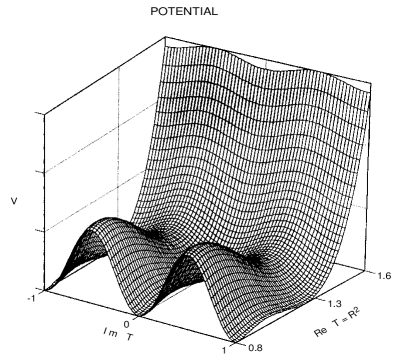
Figure 3: The $T$-duality invariant potential from gaugino condensation. Notice that the potential blows-up at large compactification radius and the minimum is at small radius ($R^{2}\sim 1.2$ in string units) as desired.

This mechanism however did not help in changing the runaway behaviour of the potential in the direction of $S$. There is a very generic problem emphasized mostly by Dine and Seiberg [83] . It is known that because at large $S$ the string is weakly coupled, the potential has to vanish asymptotically (towards a free theory). Any other minimum has to be at strong coupling for which the perturbation expansion does not work, unless there is an extra parameter that could be tuned. Such a mechanism was proposed in [84]. For stabilizing $S$, the proposal was to consider gaugino condensation of a nonsemisimple gauge group, inducing a sum of exponentials in the superpotential $W(S)\sim\sum_{i}{\alpha_{i}\exp(-3S/8\pi b_{i})}$ which can conspire to generate a local minimum for $S$ [84]. The role of the extra parameter can be played by the ratio of beta function coefficients of the different groups. These have been named ‘racetrack’ models in the recent literature.

It was later found that combining the previous ideas, together with the addition of matter fields in the hidden sector (natural in many string models)[85, 86], was sufficient to find a minimum with almost all the right properties, namely, $S$ and $T$ fixed at the desired value, $S_{R}\sim 25,T_{R}\sim 1$, supersymmetry broken at a small scale ($\sim 10^{2-4}$ GeV) in the observable sector, etc. This lead to studies of the induced soft breaking terms at low energies. Besides that relative success there are several problems that assure us that we are far from a satisfactory description of these issues

(i)

Unlike the case for $T$, fixing the $vev$ of the dilaton field $S$, at the phenomenologically interesting value, is not achieved in a satisfactory way. The conspiracy of several condensates with hidden matter to generate a local minimum at a good value, requires certain amount of fine tunning and cannot be called natural. One of the motivations for proposing the existence of a $S$-duality was precisely to find a way in which the vev of $S$ could be fixed in a natural way as it happens for $T$ [9]. More recently, there have been attempts to combine gaugino condensation with $S$ duality [88], in which $S$ can be fixed at a selfdual point $S=i,e^{i\pi/6}$; but, besides the present ignorance of how $S$-duality can be realized in 4D effective actions, there is also an unjustified assumption that this effect will provide the dominant non-perturbative correction to the superpotential (see for instance [74]  for a discussion of these points). Possible arguments for this to be the case were given in [89]. There, it was also proposed to use the recently found non-perturbative behaviour of string models, of the form $e^{-1/g}$ [53] (rather than the field theoretical $e^{-1/g^{2}}$). These corrections in the Kähler potential can in principle combine with a superpotential like that of eqs. (42,43), to fix the value of $S$. There is no yet a concrete case where these ideas are realized, though.

(ii)

The cosmological constant turns out to be always negative, which looks like an unsourmountable problem at present. This also makes the analysis of soft breaking terms less reliable, because in order to talk about them, a constant piece has to be added to the Lagrangian that cancels the cosmological constant. It is then hard to believe that the unknown mechanism generating this term would leave the results on soft breaking terms (such as the smallness of gaugino masses) untouched.

(iii)

Finally, even if the previous problems were solved, there are at least two serious cosmological problems for the gaugino condensation scenario. First, it was found under very general grounds, that it was not possible to get inflation with the type of dilaton potentials obtained from gaugino condensation [90]. Second is the so-called ‘cosmological moduli problem’ which applies to any (non-renormalizble) hidden sector scenario including gaugino condensation [92, 91]. In this case, it can be shown that if the same effect that fixes the vev’s of the moduli, also breaks supersymmetry, then: the moduli and dilaton fields acquire masses of the electroweak scale ($\sim 10^{2}$ GeV) after supersymmetry breaking [91]. Therefore if stable, they overclose the universe, if unstable, they destroy nucleosynthesis by their late decay, since they only have gravitational strength interactions. At present there is no satisfactory explanation of this problem and it stands as one of the unsolved generic problems of string phenomenology.

Soft SUSY Breaking Terms

It was found many years ago that some terms can be added to a supersymmetric lagrangian that do not respect supersymmetry but still keep the soft ultraviolet behaviour of the theory. These are the soft-breaking terms. They are naturally generated after supersymmetry breaking in general supergravity models and correspond to the following terms :

(i) Scalar masses, implying that the scalars such as squarks, become usually heavier than the fermions of the same multiplet. These are terms in the Lagrangian of the form $m_{I}^{2}\left|Q^{I}\right|^{2}$.

(ii) Gaugino masses $M_{a}\lambda^{a}\lambda^{a}$ splitting the gauge multiplets.

(iii)Cubic $A$ terms. Cubic scalar terms in the potential related to Yukawa couplings and controlled by arbitrary dimensionfull coefficients ($A$) of order the gravitino mass.

(iv)The $B$-term. A quadratic term in the potential for the scalars of the form $B\mu H\overline{H}$ where $H,\overline{H}$ represent the Higgs fields and $\mu$ is a constant that gives rise to a term in the original superpotential $W=\mu H\overline{H}$ which is allowed by all the symmetries of the minimal supersymmetric standard model. Since $\mu$ is a dimensionfull parameter it causes a problem to introduce it in the supersymmetric Lagrangian since it has to be of the order of the gravitino mass and there is no reason that a term in the supersymmetric lagrangian knows the scale of the breaking of supersymmetry.This is known as the $\mu$ problem and several solutions have been proposed. Depending on the proposed solution there is an expression for the parameter $B$ after supersymmetry breaking. In particular, if $Z\neq 0$ in eq. (21), it can be seen that the $\mu$ term is generated after supersymmetry breaking. Some calculations have shown that there are models for which $Z\neq 0$ (for recent discussions see [44, 94] ).

In this section we will follow the following strategy. Treat the supersymmetry breaking mechanism as a black box, but based on the experience with gaugino condensation, use that the end result of this mechanism is to induce nonvanishing values to the auxiliary fields of the moduli or dilaton fields. Therefore we can parametrize our ignorance of the particular breaking mechanism by working with general values of these auxiliary fields. Let us for simplicity treat a single modulus field $T$ and the dilaton $S$. But the analysis has been done in more general cases [95, 59, 96, 97]. We can then write the goldstino field (Goldstone fermion eaten by the gravitino in the process of supersymmetry breaking) as a linear combination of the fermionic components of $S$ and $T$ [97]:

$$\tilde{\eta}=\sin\theta\,\tilde{S}+\cos\theta\,\tilde{T}$$ (44)

where the goldstino angle $\theta$ mixing $\tilde{S}$ and $\tilde{T}$ describes the relative contribution of $S$ and $T$ to the breaking of supersymmetry. The general procedure for extracting the soft breaking terms is clear. We start with the supersymmetric lagrangian and substitute in it the nonvanishing auxiliary fields ($\sim e^{K/M_{p}^{2}}K^{-1/2}_{z\overline{z}}D_{z}W$), using expression (44). Performing the so called flat space limit in which $M_{p}\rightarrow\infty$ with fixed gravitino mass $m_{3/2}$ (representing the nonvanishing vev’s of the auxiliary fields and parametrizing the breaking of supersymmetry. We end up with the following values for the soft breaking parameters [97]:

$$m_{I}^{2} = m_{3/2}^{2}\left(1+n_{I}\cos^{2}\theta\right)$$

$$M^{a} = \sqrt{3}m_{3/2}\sin\theta$$

$$A_{IJK} = -\sqrt{3}m_{3/2}\left(\sin\theta+\cos\theta(n_{I}+n_{J}+n_{K})\right)$$ (45)

From this we can extract several conclusions. The dilaton dominated scenario for which $\sin\theta=1$, the soft breaking parameters are universal!This is a very appealing result explaining one of the less justified assumptions of the minimal supersymmetric standard model. On the other hand, this scenario is so restrictive that it is relatively easy to rule it out. Something that was claimed recently after comparison with the value of the top quark mass, using a particular solution of the $\mu$ problem above (see for instance [94] for a recent discussion). The importance of this scenario is that eqs (45) for $\sin\theta=1$ are valid in general and not only for orbifold models. For arbitrary mixing angle, the soft breaking terms are not necessarily universal (unless special values of the modular weights are taken). In that case we have to confront problems with flavour changing neutral currents [97]. Another conclusion we can extract from the form of the soft breaking terms is that for negative modular weights, we can get tachyons in the spectrum, for certain values of the mixing angle. The same condition that avoids tachyons, implies that the gaugino masses have to be bigger than the scalar masses, unless both vanish; in that case loop corrections may be important to determine the relative masses.

Scenarios for SUSY Breaking

The results of the previous sections have shown us that the general results extracted in the past years about gaugino condensation in string models, in terms of the field $S$, are robust. We have seen how gaugino condensation can in principle lift the string vacuum degeneracy and break supersymmetry at low energies (modulo the problems mentioned before). But this is a very particular field theoretical mechanism and it would be surprising that other nonperturbative effects at the Planck scale could be completely irrelevant for these issues. In general we should always consider the two types of nonperturbative effects:stringy (at the Planck scale) and field theoretical (like gaugino condensation). Four different scenarios can be considered depending on which class of mechanism solves each of the two problems:lifting the vacuum degeneracy and breaking supersymmetry.

For breaking supersymmetry at low energies, we expect that a field theoretical effect should be dominant in order to generate the hierarchy of scales (it is hard to believe that a nonperturbative effect at the Planck scale could generate the Weinberg-Salam scale). We are then left with two preferred scenarios: either the dominant nonperturbative effects are field theoretical, solving both problems simultaneously, or there is a ‘two steps’ scenario in which stringy effects dominate to lift vacuum degeneracy and field theory effects dominate to break supersymmetry. The first scenario has been the only one considered so far, it includes gaugino condensation and also the discussion of the previous section in terms of field-dependent soft breaking terms. The main reason this is the only scenario considered so far is that we can control field theoretical nonperturbative effects but not the stringy. In this scenario, independent of the particular mechanism, we have to face the cosmological moduli problem.

In the two steps scenario the dilaton and moduli fields are fixed at high energies with a mass $\sim M_{Planck}$ thus avoiding the cosmological moduli problem. It is also reasonable to expect that Planck scale effects can generate a potential for $S$ and $T$. The problem resides in the implementaion of this scenario [98, 74], mainly due to our ignorance of nonperturbative string effects.

In the two steps scenario, after we have fixed the vev of the moduli by stringy effects, it remains the question of how supersymmetry is broken at low energies. Notice that we would be left with the situation present before the advent of string theory in which the gauge coupling is field independent. In that case we know from Witten’s index that gaugino condensation cannot break global supersymmetry. Since there are no ‘moduli’ fields with large vev’s, the supergravity correction should be negligible because we are working at energies much smaller than $M_{Planck}$.

In fact we can perform a calculation by setting $S$ to a constant in eq. (41), it is straightforward to show that supersymmetry is still unbroken in that case [98], as expected. A more general way to see this is computing explicitly the $1/M_{Planck}$ correction to a global supersymmetric solution $W_{\phi}=0$, and see that it coincides with the solution of $W_{\phi}+WK_{\phi}/M_{p}^{2}=0$ which is always a supersymmetric extremum of the supergravity scalar potential.

There seems to be however a counterexample in the literature [73], where supersymmetry was found to be broken with vanishing cosmological constant in supergravity but unbroken in global supersymmetry. Nevertheless it can be seen that in that case, the global limit is such that $K_{UU^{*}}$ vanishes, and so the kinetic energy for $U$. This makes the corresponding minimum in the global case ill defined, since there may be other nonconstant field configurations with vanishing energy. This is then not a counterexample, because the global theory is not well defined in the minimum.

We are then left with a situation that if global supersymmetry is unbroken, we cannot break local supersymmetry, unless there are moduli like fields. If we insist to have the two steps scenario, this can bring us further back to the past and reconsider models with dynamical breaking of global supersymmetry. These models are not only very complicated but have some phenomenological problems that need to be addressed before they can be taken as valid alternatives, in particular, issues related with small gaugino masses and the value of the $\mu$ parameter are not naturally solved in these models. Nevertheless, in view of the cosmological moduli problem and because of the recent progress in understanding $N=1$ field theories, these models are attracting attention recently and, hopefully, some progress will be made (for a recent discussion with new insights see [99] ).

Therefore, there is not yet a compelling scenario for supersymmetry breaking and the field remains open, but now we have a much better perspective on the relevant issues. The nonrenormalizable hidden sector models of which the gaugino condensation is a particular case, may need a convincing solution of the cosmological moduli problem to still be considered viable. Hopefully, this will lead to interesting feedback between cosmology and string theory [100] . Furthermore, the recent progress in understanding supersymmetric gauge theories can be of much use for reconsidering gaugino condensation with hidden matter, the discussion in the string literature is far from complete. The understanding of models with chiral matter could also provide new insights to global supersymmetry breaking, relevant to the two steps scenario mentioned above.

Outlook

We have seen that the field of string phenomenology has been very animated during the past ten years and that a lot of progress has been achieved. There is a very natural justification for this kind of research, namely to look for a connection between string theory and physics. Nevertheless we have seen that this field has also contributed enormously to the progress towards formulating string theory itself. It has been claimed that string theory is currently in a similar situation as particle physics was in the early sixties, in the sense that there are a lot of experiments without a theory [53]. The only difference is that in string theory, the ‘experiments’ are just the data we have from string model building. These data have been fundamental in the discovery of $T$-duality and mirror symmetry in string theory, furthermore, the conjectured $S$-duality [9], which relates strong to weak coupling in string theory, was also originated by asking phenomenological questions. A symmetry of this sort was also fundamental to exactly solve $N=2$ field theories, even at the non-perturbative level, in the impressive work of Seiberg and Witten that lead to the understanding of confinement in a non-trivial 4D field theory[102]. Even though that result was independent of string theory, the full mathematical treatment was inherited from recent progress in string compactifications, in particular the study of mirror symmetries and $T$-duality in Calabi-Yau compactifications.

We mentioned in the introduction that there are five consistent superstring theories and each has thousands or millions of different vacua. It is now believed that the five string theories are related by strong-weak coupling dualities and furthermore, they appear to be different limits of a single underlying fundamental theory, probably in 11D, the $M$ theory (probably related with membranes or higher dimensional objects such as five-branes), which is yet to be constructed. If this is true it may solve the arbitrariness in the number of fundamental string theories by deriving them from a single theory. Furthermore, recent work based on comparison of string compactifications with the Seiberg-Witten theory, has lead to the conclusion that many and probably all Calabi-Yau compactifications are connected. Then it seems that not only the five different theories are unified, but also all the vacua of these theories are unified: since, if they are all connected, we can foresee a mechanism that lifts the degeneracy and select one point in the web of compactifications, something it could not have been done before because they were thought to be disconnected vacua and there was no way to select one. Also the Seiberg-Witten results were reproduced from a field theory approximation of a particular string vacuum, assuming $S$ duality to hold. Since the Seiberg-Witten results are robust, this is a non-trivial test for the existence of $S$ duality in string theories (for a recent review see [53] ).

We can see that we are living exciting times in string theory, where not only strings but also higher-dimensional objects are emerging as different pieces of an underlying fundamental theory. In that sense we can repeat the famous phrase of Weinberg [103]: The more the Universe seems comprehensible, the more it seems pointless; but in a less nostalgic fashion, claiming that the universe looks point-less but full of higher-dimensional objects such as strings! On the other hand the current optimism for this theory should be taken in the right perspective, none of these achievements can substitute a solid experimental test of the theory, something which may still be very far in the future. However we might be lucky and some discoveries at current and future accelerators, as well as some possible astrophysical results, could provide important clues on the validity of string theory.

Acknowledgements

I thank the organizers of the conference for providing the opportunity to give these lectures. I would also like to acknowledge my collaborators during the last few years who have influenced my understanding of this subject. Finally I would like to thank useful conversations with L.E. Ibáñez, S.-J. Rey and J. Russo that influenced the way the subjects were presented.

References

References

- [1] For a modern discussion see for instance: S. Weinberg, The Quantum Theory of Fields Vol. 1. Foundations. Cambridge University Press (1995).
-
[2]
For reviews of supersymmetry phenomenology see:
H.P. Nilles, Phys. Rep. 110 (1984) 1;
R. Arnowitt, A. Chamsedine, P. Nath, Applied N=1 Supergravity. World Scientific, Singapore (1984);
H. Haber and G. Kane, Phys. Rep. 117 (1985) 75. -
[3]
M. Green, J. Schwarz and E. Witten,
Superstring Theory, volumes 1,2,
Cambridge University Press (1987);
M. Kaku, String Theory Springer-Verlag (1988);
D. Lüst and S. Theisen, Lectures in String Theory, Springer Lecture Notes in Physics, Vol. 346 (1989);
P. Ginsparg, Les Houches Lectures Elsevier (1989);
J. Polchinski, Les Houches Lectures, hep-th/9411028 and book to appear. - [4] B. Schellekens, Superstring Construction, North-Holland (1989).
- [5] M. Dine, String Theory in Four Dimensions, North-Holland (1988).
-
[6]
L.E. Ibáñez, Lectures at ASI, St. Croix, Virgin Islands (1988);
G.G. Ross, Lectures at Banff Summer Institute (1988);
B.R. Greene, Lectures at Trieste Summer School (1990);
S. Ferrara and S. Theisen, Lectures at third Hellenic School, Corfu (1989);
L.E. Ibáñez, hep-th/9112050; hep-th/9505098;
I. Antoniadis, hep-th/9307002;
M. Dine, hep-ph/9309319;
A.E. Faraggi, hep-ph/9405357;
J.D. Lykken, hep-ph/9511456;
C. Kounnas, hep-th/9512034;
Z. Kakushadze and S.-H.H. Tye, hep-th/9512155;
J. Lopez, hep-ph/9601208;
K.R. Dienes, hep-th/9602045 and references therein. - [7] A. Giveon, M. Porrati and E. Rabinovici, Phys. Rep. 244 (1994) 77.
-
[8]
K.S. Narain, Phys. Lett. B41 (1986);
K.S. Narain,M.H. Sarmadi and E. Witten, Nucl. Phys. B279 (1987) 369;
P. Ginsparg, Phys. Rev. D35 (1987) 648. -
[9]
A. Font, L.E. Ibáñez, D. Lüst, F.
Quevedo, Phys. Lett. 249B (1990) 35;
S.-J. Rey, Phys. Rev. D43 (1991) 526;
A. Sen, Phys. Lett. B303 (1993) 22; Phys. Lett. B329 (1994) 217;
J. Schwarz and A. Sen, Nucl. Phys. B411 (1994) 35. -
[10]
L. Dixon, J. Harvey, C. Vafa and E. Witten,
Nucl.Phys. B261 (1985) 678; B274 (1986) 285;
L.E. Ibáñez, J. Mas, H.P. Nilles and F. Quevedo, Nucl. Phys. B301 (1988) 157. -
[11]
A. Font, L.E. Ibáñez and F. Quevedo,
Phys. Lett. B217 (1989) 272;
Y. Katsuki, Y. Kawamura, T. Kobayashi and N. Ohtsubo, Phys. Lett. B212 (1988) 339; Prog. Theor. Phys. (1989) 82;
Y. Katsuki, Y. Kawamura, T. Kobayashi, Y. Ono, K. Tanioka and N. Ohtsubo, Nucl. Phys. B341 (1990) 611; Phys. Lett. B227 (1989) 381. - [12] L.E. Ibáñez, H.P. Nilles and F. Quevedo, Phys. Lett. B187 (1987) 25; Phys. Lett. B192 (1987) 332.
-
[13]
K.S. Narain, M. Sarmadi and C. Vafa,
Nucl. Phys. B288 (1987) 551;
A.H. Chamseddine, J.P. Derendinger, M. Quiros, Nucl.Phys. B326 (1989) 497. -
[14]
M. Cvetič, in Proceedings of Intl. Workshop
on Superstrings, World Scientific, Singapore (1987); Phys. Rev. Lett. 59 (1987) 1795;
A. Font, L.E. Ibáñez, H.P. Nilles and F. Quevedo, Nucl. Phys. B307 (1988) 109. -
[15]
L.E. Ibáñez, J.E. Kim, H.P. Nilles and F. Quevedo,
Phys. Lett. B191 (1987) 282;
J.A. Casas and C. Muñoz, Phys. Lett. B209 (1988) 214; B214 (1988) 157;
A. Font, L.E. Ibáñez, H.P. Nilles and F. Quevedo, Phys. Lett. B210 (1988) 101;
A. Chamseddine and M. Quirós, Phys. Lett. B212 (1988) 343; Nucl. Phys. B316 (1989) 101;
A. Font, L.E. Ibáñez, F. Quevedo and Sierra, Nucl. Phys. B331 (1990) 421. -
[16]
P. Candelas, G. Horowitz, A. Strominger and E. Witten,
Nucl. Phys. B258 (1985) 46;
T. Hübsch, Calabi-Yau Manifolds: a Bestiary for Physicists, World Scientific (1992). -
[17]
See for instance:
S.-T. Yau (Ed.), Essays on Mirror Symmetry,
Intl. Press. Hong-Kong (1992);
B.R. Greene and M.R. Plesser, hep-th/9110014;
S. Hosono, A. Klemm and S. Theisen, hep-th/9403096;
T.-M. Chiang and B.R. Greene, hep-th/9509049. -
[18]
P. Candelas, X. de la Ossa, P. Green and L. Parkes,
Nucl. Phys. B359 (1991) 21;
A. Font Nucl. Phys. B391 (1993) 358;
D. Morrison, hep-th/9111025;
A. Klemm and S. Theisen Nucl. Phys. B389 (1993) 153;
P. Berglund, P. Candelas, X. de la Ossa, A. Font, T. Hubsch, D. Jancic and F. Quevedo, Nucl. Phys. B419 (1994) 352, hep-th/9308005;
P. Berglund, E. Derrick, T. Hübsch and D. Jancic hep-th/9311143 Nucl. Phys. B420 (1994) 268. -
[19]
C. Vafa and N. Warner, Phys. Lett. B218 (1989) 51;
B. Greene, C. Vafa and N. Warner, Nucl. Phys. B324 (1989) 371;
E. Martinec, in Brink, L. (ed.) et al.: Physics and Mathematics of Strings;
E. Witten, Nucl. Phys. B403 (1993) 159. - [20] B. Greene, K. Kirklin, P. Miron and G. Ross, Nucl. Phys. B278 (1986) 667; Nucl. Phys. B292 (1987) 602.
- [21] M. Cvetič and P. Langacker, hep-ph/9602424.
- [22] E. Witten, Nucl. Phys. B268 (1986) 79.
-
[23]
H. Kawai, D. Lewellen and H. Tye, Nucl. Phys. B288 (1987) 1;
I. Antoniadis, C. Bachas and C. Kounnas, Nucl. Phys. B289 (1987) 87. -
[24]
I. Antoniadis, J. Ellis, J. Hagelin and D. Nanopoulos,
Phys. Lett. B231 (1989) 65;
J. Lopez, D. Nanopoulos and K. Yuan, Nucl.Phys. B399 (1993) 654;
A. Faraggi, Phys. Lett. B274 (1992) 47; Nucl. Phys. B387 (1992) 239;
S. Chaudhuri, G, Hockney and J. Lykken, hep-th/9510241. J. Lopez, D.V. Nanopoulos and A. Zichichi, hep-ph/9601261. - [25] W. Lerche, D. Lüst and B. Schellekens, Nucl. Phys. B287 (1987) 477.
-
[26]
D. Gepner, Nucl. Phys. B296 (1988) 757; Phys. Lett. B199 (1987) 380;
A. Lütken and G. Ross, Phys. Lett. B213 (1988) 512;
Y. Kazama and H. Suzuki, Nucl. Phys. B321 (1989) 232;
A. Font, L.E. Ibáñez and F. Quevedo, Phys. Lett. B224 (1989) 79. - [27] B.E. Nilsson, P. Roberts and P. Salomonson, Phys. Lett. B222 (1989) 35.
-
[28]
A. Font, L.E. Ibáñez, M. Mondragón, G. Ross and F. Quevedo,
Phys. Lett. B227 (1989) 34;
A. Font, L.E. Ibáñez, F. Quevedo and A. Sierra, Nucl. Phys. B331 (1990) 421;
P. Berglund, C. Johnson, S. Kachru and P. Zaugg, hep-th/9509170. -
[29]
S. Cecotti, S. Ferrara and M. Villasante, Int. J. Mod. Phys. A2 (1987) 1839;
P. Binétruy, G. Girardi and R. Grimm, Phys. Lett. B265 (1991);
P. Adamietz, P. Binétruy, G. Girardi and Grimm, Nucl. Phys. B401 (1993) 257. - [30] J.-P. Derendinger, F. Quevedo and M. Quirós, Nucl. Phys. B428 (1994) 282.
- [31] E. Cremmer, S. Ferrara, L. Girardello and A. Van Proeyen, Phys. Lett. B116 (1982) 231; Nucl. Phys. B212 (1983) 413.
- [32] J. Bagger and E. Witten, Phys. Lett. 115B (1982) 202.
-
[33]
E. Witten, Phys. Lett. B155 (1985) 151;
S. Ferrara, C. Kounnas and M. Porrati, Phys. Lett. 181B (1986) 263;
J.-P. Derendinger, L.E. Ibáñez and H.P. Nilles, Nucl. Phys. B267 (1986) 365. - [34] C.P. Burgess, A. Font and F. Quevedo, Nucl. Phys. B272 (1986) 661.
-
[35]
M. Dine, N. Seiberg , X.G. Wen and E. Witten,
Nucl.Phys. B278(1986) 769; Nucl. Phys. B289 (1987) 319;
M. Cvetič, Phys. Rev. Lett. 59 (1987) 1795. -
[36]
S. Ferrara, D. Lüst, A. Shapere and S. Theisen, Phys. Lett. B225 (1989)363;
E. Chun, J. Mas, J. Lauer and H.P. Nilles, Phys. Lett. 233B (1989) 141. -
[37]
S. Hamidi and C. Vafa, Nucl. Phys. B279 (1987) 465;
L. Dixon, D. Friedan, E. Martinec and S. Shenker, Nucl. Phys. B282 (1987) 13. - [38] M. Dine and N. Seiberg, Phys. Rev. Lett. 55 (1985) 366.
- [39] L. Dixon in G. Furlan et al (eds.), Superstrings, Unified Theories and Cosmology, World Scientific, (1988).
-
[40]
E. Cremmer, S. Ferrara, C. Kounnas and D.V. Nanopoulos;
Phys. Lett. B133 (1983) 61;
J. Ellis, C. Kounnas and D.V. Nanopoulos;
Nucl.Phys. B241 (1984) 406; B247 (1984) 373;
J. Ellis, A.B. Lahanas, D.V. Nanopoulos and K. Tamvakis, Phys. Lett. B134 (1984). -
[41]
L. Dixon, V. Kaplunovsky and J. Louis, Nucl. Phys. B329 (1990) 27.
See also: M. Cvetič, J. Louis and B. Ovrut, Phys. Lett. B206 (1988) 227;
M. Cvetič, J. Molera and B. Ovrut, Phys. Rev. D40 (1989) 1140;
S. Cecotti, S. Ferrara and L. Girardello, Nucl. Phys. B308 (1988) 263. -
[42]
N. Seiberg, Nucl. Phys. B303 (1988), 286;
S. Cecotti, S. Ferrara and L. Girardello, Int. J. Mod. Phys. A4 (1989) 2475; Phys. Lett. B213 (1988) 443;
S. Ferrara and A. Strominger, contribution to Strings 89 workshop (1989). -
[43]
B. de Wit and A. Van Proeyen, Nucl. Phys. B245 (1984);
E. Cremmer, C. Kounnas, A. Van Proeyen, J.-P. Derendinger, S. Ferrara, B. de Wit and L. Girardello, Nucl. Phys. B250 (1985) 385. - [44] I. Antoniadis, E. Gava, K.S. Narain, T.R. Taylor, Nucl. Phys. B407 (1993) 706.
- [45] J. Minahan, Nucl. Phys. B298 (1988) 36.
- [46] V. Kaplunovsky, Nucl. Phys. B 307 (1988) 145; erratum, ibid B382 (1992) 436.
-
[47]
L. Dixon, V. Kaplunovsky and J. Louis, Nucl. Phys. B355 (1991) 649;
I. Antoniadis, K. Narain and T. Taylor, Phys. Lett. B267 (1991);
I. Antoniadis, E. Gava and K. Narain, Phys. Lett. B283 (1992) 209;
D. Bailin and A. Love, Phys. Lett. B292 (1992) 315;
P. Mayr and S. Stieberger, Nucl. Phys. B407 (1993) 725, Nucl. Phys. B412 (1994) 502;
D. Bailin, A. Love, W. Sabra and S. Thomas, Phys. Lett. B320 (1994) 21, Mod. Phys. Lett. A10 (1995) 337;
E. Kiritsis and C. Kounnas, Nucl. Phys. B442 (1995) 472, hep-th/9512034. G. L. Cardoso, D. Lust, T. Mohaupt Nucl. Phys. B450 (1995) 115. - [48] V. Kaplunovsky and J. Louis, Nucl. Phys. B444 (1995) 191; hep-th/9502077.
-
[49]
L.E. Ibáñez and H.P. Nilles, Phys. Lett. 169B (1986) 354;
H.P. Nilles, Phys. Lett. 180B (1986) 240. -
[50]
J.-P. Derendinger, S. Ferrara, C. Kounnas and
F. Zwirner, Nucl. Phys. B372 (1992) 145;
G.L. Cardoso and B. Ovrut, Nucl. Phys. B369 (1992) 361; Nucl. Phys. B392 (1993) 315. - [51] I. Antoniadis, E. Gava, K.S. Narain, Nucl. Phys. B383 (1992) 93.
- [52] M.A. Shifman and A.I. Vainshtein, Nucl. Phys. B359 (1991) 571; Nucl. Phys. B277 (1986) 456.
- [53] For a recent review see: J. Polchinski, hep-th/9511157.
- [54] E. Witten, hep-th/9507121.
- [55] T. Banks, L. Dixon, D. Friedan and E. Martinec, Nucl. Phys. B299 (1988) 613.
- [56] M. Dine and N. Seiberg, Nucl. Phys. B301 (1988) 357.
- [57] T. Banks and L. Dixon, Nucl .Phys. B307 (1988) 93.
-
[58]
M. Dine and N. Seiberg, Nucl. Phys. B306 (1988) 137;
A. Font, L.E. Ibáñez, H.P. Nilles and F. Quevedo, Phys. Lett. B213 (1988) 274. - [59] L. E. Ibáñez and D. Lüst, Nucl. Phys. B382 (1992) 305.
- [60] P. Ginsparg, Phys. Lett. B197 (1987) 139.
-
[61]
L.E. Ibáñez, D. Lüst and G. Ross, Phys. Lett. B272 (1991) 251;
I. Antoniadis, J. Ellis, S. Kelley and D. Nanopoulos, Phys. Lett. B271 (1991) 31;
A. Casas and C. Muñoz, Phys. Lett. B318 (1993) 543;
L.E. Ibáñez, Phys. Lett. B318 (1993) 73. -
[62]
K. Dienes and A.E. Faraggi, Phys. Rev. Lett. 75 (1995) 2646;
Nucl. Phys. B457 (1995) 409;
M. Chemtob, hep-th/9506178;
H.P. Nilles and S. Stierberger, hep-th/9510009;
P. Petropoulos and J. Rizos, hep-th/9601037. - [63] E. Witten, hep-th/9602070.
-
[64]
D. Lewellen, Nucl. Phys. B337 (1990) 61;
A. Font, L.E. Ibáñez and F. Quevedo, Nucl. Phys. B345 (1990) 389;
G. Aldazabal, A. Font, L.E. Ibáñez and A. Uranga, Nucl. Phys. B452 (1995) 3; hep-th/9508033;
J. Ellis, J.Lopez and D. Nanopoulos, Phys. Lett. B245 (1990) 375;
S. Chaudhuri, S.-W. Chung, G. Hockney and J. Lykken, Nucl. Phys. B456 (1995) 89;
G. Cleaver, hep-th/9506006;
J. Erler, hep-th/9602032. - [65] X. Wen and E. Witten, Phys. Lett. 166B (1986) 397.
- [66] B. Schellekens, Phys. Lett. B237 (1990) 363.
-
[67]
J. Ellis, J. Lopez and D. Nanopoulos, Phys. Lett. B245 (1990)
375;
I. Antoniadis and K. Benakli, Phys. Lett. B295 219;
K. Dienes, A. Faraggi and J.March-Russel, hep-th/9510223. -
[68]
J. Scherk and J. Schwarz, Phys. Lett. B82 (1979) 60;
R. Rohm, Nucl. Phys. B237 (1984) 553;
C. Kounnas and M. Porrati, Nucl. Phys. B310 (1988) 355;
S. Ferrara, C. Kounnas, M. Porrati and F. Zwirner, Nucl. Phys. B318 (1989) 75;
I. Antoniadis, C. Bachas, D. Lewellen and T. Tomaras, Phys. Lett. B207 (1988) 441;
I. Antoniadis, Phys. Lett. B246 (1990) 377;
I. Antoniadis, C. Muñoz and M. Quirós, Nucl. Phys. B397 (1993) 515;
J. Russo and A. Tseytlin, hep-th/9508068; A. Tseytlin, hep-th/9510041. -
[69]
M. Dine, N. Seiberg and E. Witten, Nucl. Phys. B289 (1987) 585;
J. Atick, L. Dixon, A. Sen, Nucl. Phys. B292 (1987) 109;
M. Dine, I. Ichinose and N. Seiberg, Nucl. Phys. B293 (1987). - [70] E. Witten, Nucl. Phys. B188 (1981) 513; Nucl. Phys. B202 (1982) 253
-
[71]
G. Veneziano, S. Yankielowicz, Phys. Lett. 113B (1982) 231;
T. Taylor, G. Veneziano, S. Yankielowicz, Nucl. Phys. B218 (1983) 493. - [72] D. Amati, K. Konishi, Y.Meurice, G.C. Rossi, G. Veneziano, Phys. Rep. 162 (1988) 169.
- [73] H.P. Nilles, Phys. Lett. 115B (1982) 193.
- [74] F. Quevedo, hep-th/9511131.
- [75] S. Ferrara, L. Girardello, H.P. Nilles, Phys. Lett. 125B (1983) 457.
- [76] J.-P. Derendinger, L.E. Ibáñez, H.P. Nilles, Phys. Lett. 155B (1985) 65.
- [77] M. Dine, R. Rohm, N. Seiberg, E. Witten, Phys. Lett. 156B (1985) 55.
- [78] C. Kounnas, M. Porrati, Phys. Lett. 191B (1987) 91.
- [79] A. de la Macorra, G.G. Ross, Nucl. Phys. B404 (1993) 321; R. Peschanski, C. Savoy, hep-ph/9504243.
- [80] C.P. Burgess, J.-P. Derendinger, F. Quevedo and M. Quirós, hep-th/9505171.
-
[81]
A. Font, L.E. Ibáñez, D. Lüst, F.
Quevedo, Phys. Lett. 245B (1990) 401;
S. Ferrara, N. Magnoli, T. Taylor, G. Veneziano, Phys. Lett. 245B (1990) 409;
H.P. Nilles, M. Olechowski, Phys. Lett. 248B (1990) 268;
P. Binetruy, M.K. Gaillard, Phys. Lett. 253B (1991) 119. - [82] L. Dixon, V. Kaplunovsky, J. Louis, Nucl. Phys. B329 (1990) 27.
- [83] M. Dine and N. Seiberg, Phys. Lett. B162 (1985) 299.
- [84] N. Krasnikov, Phys. Lett. 193B (1987) 37; L. Dixon, in The Rice Meeting, B. Bonner, H. Miettinen, eds, World Scientific (1990); J.A. Casas, Z. Lalak, C. Muñoz, G.G. Ross, Nucl. Phys. B347 (1990) 243.
- [85] D. Lüst, T. Taylor, Phys. Lett. 253B (1991) 335.
- [86] B. de Carlos, J.A. Casas, C. Muñoz, Nucl. Phys. B399 (1993) 623.
-
[87]
C.P. Burgess, J.-P. Derendinger, F. Quevedo and
M. Quirós, Phys. Lett. 348B (1995) 428.
See also, I. Gaida, D. Lüst, Int. J. Mod. Phys. A10 (1995) 2769; hep-th/9510022;
P. Binetruy, M.K. Gaillard, T. Taylor, hep-th/9504143. -
[88]
J. Horne, G. Moore, Nucl. Phys. B432 (1994) 109;
Z. Lalak, A. Niemeyer, H.P. Nilles, Phys. Lett. 349B (1995) 99; hep-th/9503170;
P. Binetruy, M.K. Gaillard, hep-th/9506207. - [89] T. Banks, M. Dine, Phys. Rev. D50 (1994) 7454.
- [90] R. Brustein, P. Steinhardt, Phys. Lett. B302 (1993) 196.
- [91] B. de Carlos, J.A. Casas, F. Quevedo and E. Roulet, Phys. Lett. B318 (1993) 447.
-
[92]
G. Coughlan, W. Fischler, E. Kolb, S. Raby and G. Ross,
Phys. Lett. 131B (1983) 59;
J. Ellis, D. Nanopoulos and M. Quirós, Phys. Lett. B174 (1986) 176;
T. Banks, D. Kaplan, A. Nelson, Phys. Rev. D49 (1994) 779. - [93] S. Ferrara,C. Kounnas and F. Zwirner, Nucl. Phys. B429 (1994) 589; C. Kounnas, I. Pavel and F. Zwirner, Phys. Lett. B335 (1994) 403.
- [94] C. Muñoz, hep-ph/9509290.
- [95] M. Cvetič, A. Font, L.E. Ibáñez, D. Lüst, F. Quevedo, Nucl. Phys. B361 (1991) 194.
- [96] V. Kaplunovsky and J. Louis, Phys. Lett B306 (1993) 269.
-
[97]
A. Brignole, L.E. Ibáñez and C. Muñoz, Nucl. Phys. B422 (1994);
A. Brignole, L.E. Ibáñez, C. Muñoz and C. Scheich, hep-ph/9508258. - [98] C.P. Burgess, L.E. Ibáñez and F. Quevedo, unpublished (1995).
- [99] M. Dine, A. Nelson, Y.Nir, Y. Shirman, hep-ph/9507378.
-
[100]
T. Banks, M. Berkooz, G. Moore, S. Shenker, P. Steinhardt,
Phys. Rev. D52 (1995) 3548;
T. Banks, M. Berkooz, P. Steinhardt, Phys. Rev. D52 (1995) 705;
A. de la Macorra, hep-ph/9501250;
D. Lyth and E. Stewart, Phys. Rev. Lett. 75 (1995) 201; hep-ph/9510204;
T. Banks, hep-th/9601151. -
[101]
R. Brustein, M. Gasperini, M. Giovannini, G. Veneziano, hep-th/9510081;
G. Veneziano, hep-th/9512091. - [102] N. Seiberg and E. Witten, Nucl. Phys. B426 (1994) 19.
- [103] S. Weinberg, The First Three Minutes, Basic Books Inc., Publishers, New York (1977).