Variational derivation of exact skein relations from Chern–Simons theories

Abstract

The expectation value of a Wilson loop in a Chern–Simons theory is a knot invariant. Its skein relations have been derived in a variety of ways, including variational methods in which small deformations of the loop are made and the changes evaluated. The latter method only allowed to obtain approximate expressions for the skein relations. We present a generalization of this idea that allows to compute the exact form of the skein relations. Moreover, it requires to generalize the resulting knot invariants to intersecting knots and links in a manner consistent with the Mandelstam identities satisfied by the Wilson loops. This allows for the first time to derive the full expression for knot invariants that are suitable candidates for quantum states of gravity (and supergravity) in the loop representation. The new approach leads to several new insights in intersecting knot theory, in particular the role of non-planar intersections and intersections with kinks.

I Introduction

Witten [1] realized some years ago that the expectation value of a Wilson loop $W(\gamma)$ in a Chern–Simons theory was a knot invariant. This follows from the fact that Chern–Simons theories are diffeomorphism invariant and that the Wilson loops are observables for such theories, having therefore diffeomorphism invariant expectation values. The resulting knot invariant is the Kauffman bracket [2] for the case of an $SU(2)$ Chern–Simons theory and for the case of $SU(N)$ is a regular isotopic polynomial associated with the HOMFLY [3] polynomial. These results were derived based on the calculations of Moore and Seiberg [4] for the monodromies of rational conformal field theories. The knowledge of the Yang-Baxter relations satisfied by the monodromies translates immediately into skein relations for the polynomial in question.

Independently, Smolin [5] and later Cotta-Ramusino, Guadagnini, Martellini and Mintchev [6] noted that a simpler heuristic derivation of the skein relations was possible. The idea is similar to the Makeenko-Migdal [7] approach to Yang–Mills theories. It is based on studying the changes in the expectation value of the Wilson loop when one performs small deformations. This calculation can be done explicitly to first order in the deformation. The results can be interpreted as skein relations to first order in the inverse coupling constant of the theory, which is tantamount to determining the knot polynomial to first order.

The latter method is quick and computationally efficient, and has a simple generalization to the case of intersecting loops [8, 9]. The main drawback, especially in the case where the result is not known by other methods, is that one only gets the skein relations to first order in the inverse of the coupling constant of the theory. It is therefore of interest to find a suitable generalization that would yield the exact skein relations to all orders. This is the main purpose of this paper.

On the other hand, the subject of intersecting knot invariants has received little attention and is of paramount importance for the construction of quantum states of gravity in the loop representation [10, 11]. In this approach, based on the canonical quantization of general relativity in terms of Ashtekar variables [12], wavefunctions are knot invariants due to the diffeomorphism symmetry of general relativity [13]. The Hamiltonian constraint has only a non-trivial action at intersections [14]. Only intersecting knots are associated with non-degenerate spacetimes [15]. Whenever one generalizes an invariant of smooth loops to take values on intersecting loops there is generically freedom in how the invariant is defined, as long as it is compatible with the Reidemeister moves. However, in the case of quantum gravity, wavefunctions have to be compatible with a set of constraints among functions of loops known as the Mandelstam identities. These identities naturally involve intersecting loops and severely limit the possible generalizations of invariants to intersections. We will show in this paper how to generalize the invariants stemming from Chern–Simons theory to be compatible in an exact way with the Mandelstam identities. This in particular also defines the values of the invariants for multicomponent links. This is of particular relevance for quantum gravity since it is known that the exponential of the Chern–Simons form built from the Ashtekar connection is an exact solution to all the constraints of quantum gravity [17, 8]. If one wishes to find the counterpart of this state in the loop representation one ends up computing exactly the same integral as the expectation value of a Wilson loop in a Chern–Simons theory.

One additional motivation for the construction we present is that the Chern–Simons state not only arises in canonically quantized vacuum general relativity but also in other contexts, like Einstein–Yang–Mills theories [16] and supergravity [18]. In these cases the (super)gauge group of the associated Chern–Simons theory differs from that of gravity and therefore so do the resulting invariants. In the particular case of supergravity the resulting invariant had not been computed by other means, and turns out to be associated with the Dubrovnik–Kauffman polynomial [19].

A first attempt to obtaining a finite prescription from variational calculations was made by Brügmann [20]. In particular, the idea of exponentiating the infinitesimal transformation was presented there. Because of ambiguities in the formulation presented in that paper, one could only check, given the exact skein relations, that they were compatible with the formulation. Here we add two key elements that make the construction a well defined prescription: on the one hand we offer a justification of why can the infinitesimal results be exponentiated; on the other hand we make crucial use of the Mandelstam identities to uniquely fix a prescription for the exponentiation. The prescription now allows, in a case where one does not know the result beforehand, to compute the resulting polynomial.

The organization of this article is as follows. In the next section we will discuss, using the non-Abelian Stokes theorem, how to perform a finite deformation of the expectation value of the Wilson loop.In section III we discuss the deformation of twists and kinks and in section IV of planar and non-planar intersections. We discuss the implications of the results in section V.

II The non-Abelian Stokes theorem and finite deformations of loops

One is interested in establishing skein relations for the following function of a loop,

$$<W(\gamma)>=\int dA\exp\left({ik\over 4\pi}S_{CS}\right)W(\gamma)$$ (1)

where

$$W(\gamma)={\rm Tr}\left[{\rm P}\exp\left(i\oint dy^{a}A_{a}(y)\right)\right]$$ (2)

where $\gamma$ is a closed curve in a three manifold, $A_{a}$ is a connection in a semi-simple Lie algebra and $S_{CS}$ is the action of a Chern–Simons theory,

$$S_{CS}=\int d^{3}x\,\epsilon^{abc}{\rm Tr}[A_{a}\partial_{b}A_{c}-{2\over 3}iA_{a}A_{b}A_{c}].$$ (3)

Finding skein relations involves relating the value of the $<W(\gamma)>$ for different loops. These loops are determined by the replacement of over-crossings by under-crossings in a planar projection. Skein relations also arise between a loop with and without a twist, over-crossings and intersections. The usual notation for the several types of crossings is shown in figure 1. We will see later on that the consideration of invariants with intersections requires several other crossings. For instance, the skein relations that define the Kauffman bracket knot polynomial on loops without intersections are,

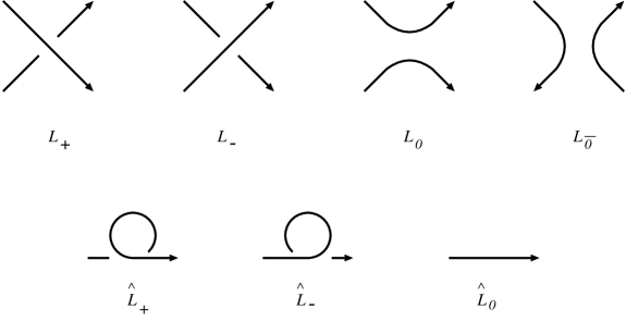
FIG. 1.: The different crossings involved in the skein relations for invariants of non-intersecting loops

$$K(\hat{L}_{+}) = q^{3/4}K(\hat{L}_{0})$$ (4)

$$K(\hat{L}_{-}) = q^{-3/4}K(\hat{L}_{0})$$ (5)

$$q^{1/4}K(L_{+})-q^{-1/4}K(L_{-}) = (q^{1/2}-q^{-1/2})K(L_{0})$$ (6)

$$K({\rm unknot})=1.$$ (7)

With these relations the polynomial is completely characterized for any link. What Witten [1] showed using conformal field theory techniques is that ${1\over 2}<W(\gamma)>$ satisfies the above relations. Here we will show it by performing directly deformations of the loops on the expression of the expectation value.

In order to do this, we need to study deformations of Wilson loops. Wilson loops are traces of holonomies. It turns out that the information needed to compute a holonomy is less than that present in a closed curve. Several closed curves yield the same holonomy. In this paper we will use the word “loop” to denote the equivalence class of curves that yield the same holonomy for all connections . Loops form a group structure called the group of loops [16].

It is well known that if one adds to a loop another loop of infinitesimal area, the change in the Wilson loop can be coded in terms of an infinitesimal operator in loop space called the loop derivative [16]. This is shown in figure 2. The concrete expression is,

$$W(\gamma\circ\delta\gamma)=(1+{1\over 2}\sigma^{ab}\Delta_{ab}(\pi_{o}^{x}))W(\gamma)$$ (8)

where $\circ$ denotes composition of loops, $\sigma^{ab}$ is the infinitesimal element of area of the the loop $\delta\gamma$ and $\pi_{o}^{x}$ is an open path connecting the basepoint of the loop $\gamma$ to the point $x$ at which one adds the infinitesimal loop with infinitesimal element of area $\sigma^{ab}$. Notice that the loop derivative $\Delta_{ab}$ depends on the path used to compute it and we denote so in its expression. The loop derivative is related to the infinitesimal generators of the group of loops [16].

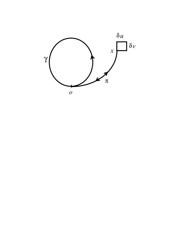
FIG. 2.: The infinitesimal loop that defines the loop derivative.

One can write [16] an expression for an operator $U(\gamma)$ that adds a finite loop $\gamma$ to a Wilson loop in terms of the loop derivative. Let $\gamma(s)$ be a parameterized curve belonging to the equivalence class defining the finite loop $\gamma$ with $s\in[0,1]$. Consider a one-parameter family of parameterized loops $\eta(s,t)$ interpolating smoothly between $\gamma(s)$ and the identity loop, such that $\eta(s,0)$ is in the equivalence class of the identity loop and $\eta(s,1)=\gamma(s)$. Consider the curves $\eta(s,1)$ ($=\gamma(s)$) and $\eta(s,1-\epsilon)$. The two curves are drawn in figure 3 and differ by an infinitesimal element of area.

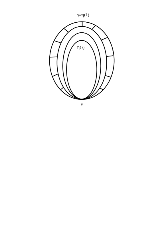
FIG. 3.: The construction of a finite loop from the loop derivative. The curves $\delta\eta_{i}$ are determined by two elements in the family $\eta(t)$.

The whole purpose of our construction will be to cover the infinitesimal area separating the two mentioned curves with a “checkerboard” of infinitesimal closed curves such that along each of them one can define a loop derivative. One can therefore express the curve $\gamma(s)$ as

$$\gamma(s)=\lim_{n\rightarrow\infty}\eta(s,1-\epsilon)\circ\delta\eta_{1}\circ\cdots\circ\delta\eta_{n},$$ (9)

where the $\delta\eta_{i}$ are shown in figure 3. Analytically, in terms of differential operators on functions of loops we can write

$$\Psi(\eta(1))= \Psi(\eta(1-\epsilon))$$ (11)

$$+\epsilon\oint_{0}^{1}ds\dot{\eta}^{a}(1-\epsilon,s){\eta^{\prime}}^{b}(1-\epsilon,s)\Delta_{ab}(\eta(1-\epsilon)_{o}^{s})\Psi(\eta(1-\epsilon)),$$

where $\dot{\eta}(t,s)\equiv d\,\eta(t,s)/dt$ and $\eta^{\prime}(t,s)\equiv d\,\eta(t,s)/ds$. It is immediate to proceed from $\eta(1-\epsilon,s)$ inwards just by repeating the same construction, and so continuing until the final curve is the identity. The end result is

$$\Psi(\gamma)={\rm T}\exp\left(\int_{0}^{1}dt\oint_{0}^{1}ds\dot{\eta}^{a}(t,s){\eta^{\prime}}^{b}(t,s)\Delta_{ab}(\eta(t)_{o}^{s})\right)\Psi(\eta(0))\equiv U(\gamma)\Psi(\eta(0))$$ (13)

where the outer integral is ordered in $t$ (T-ordered). This result is the loop version of the non-Abelian Stokes theorem of gauge theories [22] and it shows that the loop derivative is a generator of loop space, i.e., it allows us to generate any finite loop homotopic to the identity. Due to the properties of the group of loops [16], the construction is independent of the particular family of loops used to go from the identity element to the final loop $\gamma$.

It is useful to rewrite the expression of the operator $U$ as,

$$U(\gamma)={\rm T}\exp\int_{0}^{1}dt\delta(t)$$ (14)

where

$$\delta(t)=\oint_{0}^{1}ds\dot{\eta}^{a}(t,s){\eta^{\prime}}^{b}(t,s)\Delta_{ab}(\eta(t)_{o}^{s}).$$ (15)

The operator $\delta$ is closely related to the unparameterized “connection derivative” [16].

We would now like to apply the above deformation to a portion of a loop in order to construct the elements that appear in the skein relations.

III Skein relations associated to twists and kinks

A Twists

We start by the simplest skein relations, those that relate the value of the invariant with and without a twist. Starting from a regular portion of a loop $\eta_{o}^{x}$ going from the origin to $x$, one can add a twist by considering a family of loops of the form,

$$\eta^{a}(s,t)=\eta^{a}(s)+tu^{a}(s)$$ (16)

where $u^{a}(s)$ is a vector along the loop that materializes the deformation shown in figure 4.

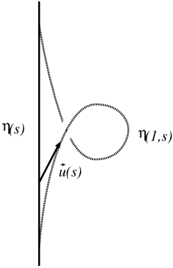
FIG. 4.: Adding a twist to a loop using the finite deformation operator

To compute the deformation, we first evaluate the action of the loop derivative on the expectation value of the Wilson loop.

$$\sigma^{ab}\Delta_{ab}(\eta(t)_{o}^{x})<W(\gamma)>=i\int dA\sigma^{ab}F_{ab}^{k}(x){\rm Tr}(\tau^{k}H(\eta(t)_{x}^{o}\circ\gamma\circ\eta(t)_{o}^{x}))e^{{ik\over 4\pi}S_{CS}}$$ (17)

where we have taken into account that the deformation is along one element of the the family of loops $\eta(t)$. $\tau^{k}$ are the generators of the algebra $su(2)$. In this calculation we have assumed that the loop derivative acts on $<W(\gamma)>$ by simply acting inside the functional integral $W(\gamma)$. This is a strong hypothesis, notice that the integral $<W(\gamma)>$ is diffeomorphism invariant and therefore the limit involved in the definition of the loop derivative is singular. We are assigning a value to that limit by permuting the functional integral and the limit involved in the loop derivative.

We now use the fact that the field tensor is the dual of the magnetic field, which can in turn be obtained through a functional derivative of the exponential of the Chern–Simons state,

$$iF_{ab}^{l}(x)e^{{ik\over 4\pi}S_{CS}}=i\epsilon_{abc}B^{c\,l}e^{{ik\over 4\pi}S_{CS}}={4\pi\over k}\epsilon_{abc}{\delta\over\delta A_{c}^{l}}e^{{ik\over 4\pi}S_{CS}}.$$ (18)

Substituting this expression in (17) and integrating the functional derivative by parts we get,

$$\sigma^{ab}\Delta_{ab}(\eta(t)_{o}^{x})<W(\gamma)>=-{4\pi\over k}\int dA\sigma^{ab}\ e^{{ik\over 4\pi}S_{CS}}\epsilon_{abc}{\delta\over\delta A_{c}^{l}}{\rm Tr}(\tau^{l}H(\eta(t)_{x}^{o}\circ\gamma\circ\eta(t)_{o}^{x}))$$ (19)

and acting with the functional derivative on the holonomy we get,

$$\sigma^{ab}\Delta_{ab}(\eta(t)_{o}^{x})<W(\gamma)>=-{4\pi i\over k}\int dA\sigma^{ab}e^{{ik\over 4\pi}S_{CS}}\epsilon_{abc}\oint_{\gamma}dy^{c}\delta^{3}(x-y){\rm Tr}\left(\tau^{l}H(\eta(t)_{x}^{o})H(\gamma_{o}^{y})\tau^{l}H(\gamma_{y}^{o})H(\eta(t)_{o}^{x})\right).$$ (20)

Notice that the previous expression is distributional, involving a one-dimensional integral of a three-dimensional Dirac delta. It is remarkable that one can use it to obtain an expression for the operator $U$ that generates finite deformations. In order to see this, we first write an expression for the operator $\delta$ associated with the deformation induced by the vector field $\vec{u}(s)$,

$$\delta_{\vec{u}}(t)<W(\gamma)>=-{4\pi i\over k}\int_{0}^{1}dsu^{a}(s)({\eta^{\prime}}^{b}(s)+t{u^{\prime}}^{b}(s))\epsilon_{abc}\oint_{\gamma}dy^{c}\delta^{3}(\eta(s,t)-y)\left<{\rm Tr}\left(\tau^{l}H(\eta(t)_{x}^{o})H(\gamma_{o}^{y})\tau^{l}H(\gamma_{y}^{o})H(\eta(t)_{o}^{x})\right)\right>.$$ (21)

In order to construct the finite deformation operator we need to exponentiate $\delta$. As is shown in appendix A, one can find a regularization such that $\delta$’s at different points commute when acting on the expectation value of the Wilson loop in Chern-Simons theory (in general they do not commute, see [16]). Therefore the $T$-ordered exponential reduces to an ordinary exponential and we get,

$$U(\gamma)=\exp\left(\int_{0}^{1}\delta_{\vec{u}}(t)dt\right)$$ (22)

when acting on $<W(\gamma)>$ and the integral in the exponent can be computed explicitly,

$$\int_{0}^{1}dt\delta_{\vec{u}}(t)<W(\gamma)>=\mp{3i\pi\over k}<W(\gamma)>$$ (23)

and the sign $\mp$ corresponds to the kind of crossing generated in the loop by the vector field $\vec{u}$. Positive sign corresponds to the right hand rule. To go from 21 to the last expression we have made use of the Fierz identity for $SU(2)$,

$$\tau^{k}{}^{A}_{B}\tau^{k}{}^{C}_{D}={1\over 2}\delta^{A}_{D}\delta^{C}_{B}-{1\over 4}\delta_{B}^{A}\delta_{D}^{C},$$ (24)

and we performed explicitly the three one-dimensional integrals. The result is the normalized oriented volume subtended by the deformation. Strictly speaking, this result implies a choice of regularization, since the type of integral that one is left with is of the form $\int_{0}^{1}dt\delta(t)$ (see [20] for details). This choice in the regularization is tantamount to introducing a new parameter in the derivation, corresponding to the value of the above integral. Throughout this paper we will take it to be unity. Otherwise, it would imply a multiplicative shift in the value of $k$.

The above expression can be summarized in terms of the notation for skein relations we introduced before as,

$$<W(\hat{L}_{+})> = \exp\left(-{3i\pi\over k}\right)<W(\hat{L}_{o})>$$ (25)

$$<W(\hat{L}_{-})> = \exp\left({3i\pi\over k}\right)<W(\hat{L}_{o})>$$ (26)

which coincide with the skein relations for the Kauffman bracket (4,5) if one makes the identification

$$q=\exp(-{4i\pi\over k}).$$ (27)

It is well known that perturbative techniques like the ones we are using here fail to capture the additive shift in the coupling constant first observed by Witten [1]. A discussion, and a proposal to amend perturbative techniques to capture this effect through a recourse to the semi-classical approximation can be found in Awada [23]. We could proceed in the same fashion here and modify the value of the coupling constant, but we will leave it as it is for simplicity.

B Kinks

A kink (discontinuity of the tangent) is a diffeomorphism invariant feature of a loop. We will now show that the expectation value of a Wilson loop in a Chern–Simons theory is not sensitive to the presence of kinks in the loop under the kind of regularization we are using in our calculations. This is an important result because it directly relates to the value of the invariant when one has intersections with kinks, which are crucial to implement the Mandelstam identities. We will discuss this at the end of this section and will see later that the choice we make for the treatment of the kinks is central to establishing consistency.

Let us consider a loop with a kink like that shown in figure 5. The kink defines a plane. We can deform the kink into a smooth section of the loop through a deformation in the plane. The calculation is exactly the same as that of a smooth section, so we will not repeat it here. The only precaution is to consider the appropriate tangent vector at both sides of the kink. The reason why we do not need more details is that since the deformation is planar, the contribution vanishes. Basically one gets a contribution similar to (21) that has three coplanar vectors contracted with the Levi–Civita symbol.

FIG. 5.: Deforming a kink into a smooth section

The case of intersections with kinks is essentially similar. There are two different types of (double) planar intersections with kinks, as shown in figure 6.

FIG. 6.: Double intersections without and with kinks

In all cases the operator $U(\gamma)$ deforms independently each line at the intersection. For the cases with kinks that means that each kink can be deformed into a smooth section. That means that in cases $L_{W}$ and $L_{\bar{W}}$ the intersection can be removed by the deformation and we get the skein relations

$$<W(L_{W})> = <W(L_{0})>$$ (28)

$$<W(L_{\bar{W})}> = <W(L_{\bar{0}})>$$ (29)

that are shown in figure 7

FIG. 7.: Skein relations for intersections with kinks

Notice that in all cases the removal of kinks at planar intersections can be accomplished given a straightforward regularization of the deformation operator. This provides a justification for the identification of $L_{W}$ with $L_{0}$ that has been used in other works [20, 24]. We will return to discuss intersections with kinks at the end of the next section, where we will analyze a deformation that produces double lines in the loop that is of interest in the context of the exponentiation of the skein relation for straight through intersections, which we discuss now.

IV Skein relations for intersections

A Infinitesimal skein relations

In the case of a “straight through” intersection (no kinks), the calculation is different than in the previously discussed cases. In this case, the Wilson loop is the trace of the product of the holonomies along the petals defined by the intersection. For instance in the case of figure 8 one could write it as $W(\gamma)={\rm Tr}(H_{12}H_{34})$.

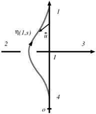
FIG. 8.: Deformation of a “straight through” intersection. The deformation vector $\vec{u}$ is perpendicular to the plane determined by the intersection

The action of the loop derivative on the holonomy is independent of the presence of the intersection, the expression is exactly the same as (17). The difference in the construction arises when one integrates by parts. Since the loop has a double point at the intersection, the functional derivative with respect to $A_{a}$ has two contributions at that point, corresponding to its action on the holonomy when it traverses that point the first and the second time. One of the contributions vanishes since it produces a term proportional to the tangent of the loop in the same plane as the deformation and therefore spans no volume. The other contribution is the one of interest. It can be written as,

$$\sigma^{ab}\Delta_{ab}(\eta(t)_{o}^{x})<W(\gamma)> = -{4\pi i\over k}\int dA\sigma^{ab}e^{{ik\over 4\pi}S_{CS}}\epsilon_{abc}\int_{\gamma_{23}}dy^{c}\delta^{3}(x-y)$$ (31)

$$\times{\rm Tr}\left(\tau^{l}H(\eta(t)_{x}^{o})H_{34}(\gamma_{o}^{I})H_{12}(\gamma_{I}^{y})\tau^{l}H_{12}(\gamma_{y}^{I})H_{34}(\gamma_{I}^{o})H(\eta(t)_{o}^{x})\right).$$

where we have assumed that the origin $o$ of the loop is in the petal $34$. We now use the Fierz identity (24) and compute the integral of the $\delta$ operator,

$$\int_{0}^{1}dt\delta_{\vec{u}}(t)<{\rm Tr}(H_{12}(\gamma)H_{34}(\gamma))>=-{i\pi\over k}{\rm Tr}(H_{12}(\gamma)H_{34}(\gamma))+{2i\pi\over k}{\rm Tr}(H_{12}(\gamma)){\rm Tr}(H_{34}(\gamma))$$ (32)

Which can be rewritten as

$$\int_{0}^{1}dt\delta_{\vec{u}}(t)<W(L_{I})>=-{i\pi\over k}<W(L_{I})>+{2i\pi\over k}<W(L_{W})>.$$ (33)

A couple of remarks are in order. First, there is a difference between equations (32) and (33), since equation (32) refers to the whole loop and equation (33) only to its intersection. The former has information about the connectivity of the loop, the latter does not. Therefore, if one is to claim that equation (33) follows from equation (32) one should prove that it does so for any connectivity. For the case of double intersections, there are only two different possible connectivities. It is straightforward to check that equation (33) holds independently of the connectivity chosen. Second, in spite of similarities to equation (6), equation (33) is only valid to first order in $1/k$ and needs to be exponentiated to obtain the skein relation. Since equation (33) shows that the action of $\delta$ mixes $L_{I}$ and $L_{W}$, in order to exponentiate it we need to compute the action of the deformation operator on $L_{W}$. Notice that this is a different deformation than the one computed in the last section, which was coplanar with the intersection. We discuss of the resulting calculation at the end of this section.

Before doing that computation, it is worthwhile observing that one could combine the Fierz identity (24) with the following identity,

$$\epsilon^{AC}\epsilon_{BD}=\delta^{A}_{B}\delta^{C}_{D}-\delta^{A}_{D}\delta^{C}_{B}$$ (34)

to get,

$$\tau^{k}{}^{A}_{B}\tau^{k}{}^{C}_{D}={1\over 4}(\delta^{A}_{D}\delta^{C}_{B}-\epsilon^{AC}\epsilon_{BD}),$$ (35)

and using this expression in (31) we get

$$\int_{0}^{1}dt\delta_{\vec{u}}(t)<{\rm Tr}(H_{12}(\gamma)H_{34}(\gamma))>={i\pi\over k}{\rm Tr}(H_{12}(\gamma)){\rm Tr}(H_{34}(\gamma))+{i\pi\over k}{\rm Tr}(H_{12}(\gamma)H_{34}^{-1}(\gamma)).$$ (36)

In contrast to (32) this expression leads to different first-order skein relation depending on the connectivity of the knot. If the the connectivity is such that the original loop has a single component, then the skein relation is,

$$\int_{0}^{1}dt\delta_{\vec{u}}(t)<W(L_{I})>={i\pi\over k}<W(L_{0})>+{i\pi\over k}<W(L_{\bar{0}})>.$$ (37)

where the element $L_{\bar{0}})$ is defined in figure 1. The interest of this skein relation stems from the fact that the original definition of the Kauffman bracket [19] was given in terms of relations of this kind. Moreover, Major and Smolin [24] used this identity to derive the binor identity from the Kauffman bracket. The original definition of the bracket differs from the one we use here in a factor $(-1)$ to elevated to the number of connected components of the loop, which fixes the connectivity difference we encountered above.

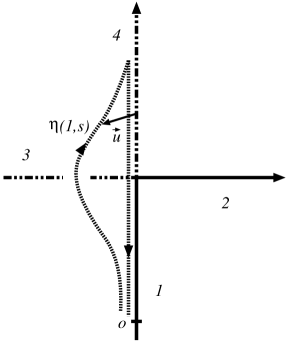
FIG. 9.: The skein relation for intersections requires the analysis of this type of deformation of an intersection with kinks.

To conclude, we discuss the deformation of an $L_{W}$ as mentioned before. We need to compute the deformation of an intersection with a kink that is shown in figure 9. The loop starts at the origin, goes through the deformation determined by the vector $\vec{u}$, which we denote with a dotted line and then traverses the petal $12$ going through the kink and ends with the petal $34$. The resulting loop has double lines. In ordinary knot theory double lines are not considered. They could be incorporated through additional sets of skein relations, as we discuss in subsection F. If one pursues a calculation similar to the ones we have been doing up to now for this case, one encounters two contributions, stemming from the volumes spanned by the deformation and the tangents to the loop at the intersection in lines $2$ or $3$. The integrals involve terms of the form $\delta^{3}(y)\Theta(y)$. The Heaviside function $\Theta(y)$ limits the integral in the contribution to the corresponding petal. Although these kinds of expressions can be regularized, there does not appear any natural way of assigning relative weights to the two contributions from the petals. The way we handle it here is to write the contribution in terms of two arbitrary factors $\alpha$ and $\beta$,

$$\int_{0}^{1}dt<W(L_{W\pm})>=\pm{i\pi\over k}\left(\alpha<W(L_{I})>+\beta<W(L_{W})>\right).$$ (38)

where we have denoted $W\pm$ the elements that result from doing the deformation up or down with respect to the plane determined by the intersection.

We will see in the next section that the arbitrary factors can be uniquely determined by the Mandelstam identities when we exponentiate the operator.

B Exponentiation and Mandelstam identities

The skein relations involving $L_{\pm}$ and $L_{I}$ are obtained studying the deformation of an intersection. In order to obtain these deformations in a finite form we need to exponentiate the differential expressions we obtained in the previous section. Specifically, we have

$$\left(\begin{array}[]{c}<W(L_{\mp})>\\ <W(L_{W\mp})>\end{array}\right)=\exp\int_{0}^{1}dt\delta_{\pm{\vec{u}}}(t)\left(\begin{array}[]{c}<W(L_{I})>\\ <W(L_{W})>\end{array}\right)=\exp\left(\pm{i\pi\over k}\right)\left(\begin{array}[]{cc}-1&2\\ \alpha&\beta\end{array}\right)\left(\begin{array}[]{c}<W(L_{I})>\\ <W(L_{W})>\end{array}\right).$$ (39)

We are interested only in computing $<W(L_{\mp})>$. We are not interested in the value of $<W(L_{W\mp})>$ since as we explained before it involves double lines, which would require a separate discussion involving extra skein relations (see subsection F). We do not know the values of $\alpha$ and $\beta$. However, since we are computing the invariant as an expectation value of a Wilson loop, we expect it to satisfy the same relations that Wilson loops satisfy: the Mandelstam identities. We will see that imposing the Mandelstam identities is enough to determine the coefficients $\alpha$ and $\beta$ uniquely and therefore to find the skein relation.

We therefore need to discuss the content of the Mandelstam identities. As we mentioned before, these identities relate the behavior of reroutings of the loops at intersections and involve non-trivial information about the connectivity of the loop. We will restrict the explicit discussion to double intersections, but it is immediate to see that suitable generalizations can be found for more complex intersections. For double intersections, one can always consider a planar diagram, and two possible routings exist, as shown in figure 10. Each routing leads to an identity. The identities,

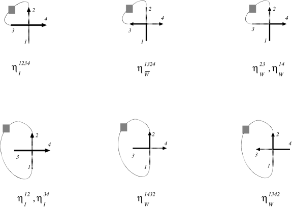
FIG. 10.: The different loops that arise in the Mandelstam identities involved in double intersections. The grey boxes denote possible knottings and interlinkings with other portions of the loop (including possible additional intersections and kinks). In order to unclutter the figures, we only denoted partial connectivities, in all cases the loops have to be closed by connecting the open strands, with no particular restrictions, i.e. the resulting petal could have knottings and interlinkings with the rest of the loop.

$$<W(\eta_{I}^{1234})>+<W(\eta_{\bar{W}}^{1324})> = <W(\eta_{W}^{23})W(\eta_{W}^{14})>$$ (40)

$$<W(\eta_{W}^{1432})>+<W(\eta_{{W}}^{1342})> = <W(\eta_{I}^{12})W(\eta_{I}^{34})>,$$ (41)

involve different loops, as shown in the figure (10). Moreover, they are valid for a completely arbitrary loop that has a double intersection. In order to use these identities to allow us to fix the arbitrary parameters in the exponentiation, we will consider —for simplicity— its expression for a particular set of loops. We will then have to check that the resulting invariant is consistent with the identities for all possible loops. The loops we wish to consider are the ones obtained by reconnecting the loops of figure (10) with direct strands, i.e. adding no knottings or interlinkings and are shown in figures 11 and 12. The Mandelstam identities for these loops are,

FIG. 11.: Schematic depiction of the first identity used to determine $\alpha$ and $\beta$.

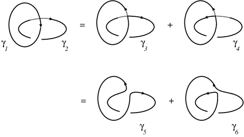
FIG. 12.: Schematic depiction of the second identity used to determine $\alpha$ and $\beta$.

$$<W(\eta_{1})>+<W(\eta_{2})>=<W(\eta_{3})W(\eta_{4})>$$ (42)

$$<W(\gamma_{3})>+<W(\gamma_{4})>=<W(\gamma_{1})W(\gamma_{2})>.$$ (43)

We now make use of the skein relations for intersections with kinks (28,29). In equation (42) this allows to replace $\eta_{2}$ by the unknot and $\eta_{3}$ and $\eta_{4}$ by the two component unlinked link. Therefore $<W(\eta_{2})>=1$.

In equation (43) the use of the skein relations is shown in figure 12 to transform $\gamma_{3}$ and $\gamma_{4}$ to the unknot with a twist added. Using the skein relations (25,26) one gets, $<W(\gamma_{5})>=q^{3\over 4}$ and $<W(\gamma_{6})>=q^{-{3\over 4}}$.

We now use (39) in combination with these expressions to determine the values of $\alpha$ and $\beta$. It turns out we only need to use the expression of the exponential that appears in (39) expanded up to second order in $1/k$. Using this expression to determine $<W(\eta_{1})>$, $<W(\gamma_{1})W(\gamma_{2})>$ and $<W(\eta_{3})W(\eta_{4})>$ one gets that $\alpha=1$ and $\beta=0$. This completely characterizes the skein relation for the intersections (39). From there we conclude that,

$$\left(\begin{array}[]{c}<W(L_{\mp})>\\ <W(L_{W\mp})>\end{array}\right)=\left(\begin{array}[]{cc}q^{\pm{1\over 4}}&(q^{\mp{1\over 4}}-q^{\pm{1\over 4}})\\ 0&q^{\mp{1\over 4}}\end{array}\right)\left(\begin{array}[]{c}<W(L_{I})>\\ <W(L_{W})>\end{array}\right).$$ (44)

From this expression, adding an subtracting with appropriate weights the expressions with the different signs, we can work out the usual skein relation for the Kauffman bracket without intersections,

$$q^{{1\over 4}}<W(L_{+})>-q^{-{1\over 4}}<W(L_{-})>=(q^{{1\over 2}}-q^{-{1\over 2}})<W(L_{0})>,$$ (45)

and also the definition of the expectation value for a planar straight through intersection,

$$<W(L_{I})>={1\over(q^{{1\over 4}}+q^{-{1\over 4}})}[<W(L_{+})>+<W(L_{-})>].$$ (46)

We therefore conclude that the expectation value of the Wilson loop in an $SU(2)$ Chern–Simons theory is, up to a factor of 2 with the conventions of this paper, identical to the Kauffman bracket knot polynomial.

C Consistency for all loops and to all orders in $1/k$

We have just shown that considering the exponential of the infinitesimal deformation to second order in $1/k$ and requiring consistency with the Mandelstam identity for a particular set of loops uniquely fixes the values of the indeterminate coefficients $\alpha$ and $\beta$ of the infinitesimal deformation. We need to check that the construction is consistent to all orders in $1/k$ and for all possible sets of loops with planar intersections. We will now show that this is the case. In order to do this, the finite version of the form of the skein relation (37), which again can be derived in the same form as the finite skein relation we derived above is useful,

$$<W(L_{\pm})>=q^{\pm{1\over 4}}<W(L_{0})>-q^{\mp{1\over 4}}<W(L_{\bar{0}})>.$$ (47)

As we mentioned before, this relation depends on the connectivity of the loop, we are assuming it is such that $L_{I}$ has one independent component, as shown in loop $\eta_{I}^{1234}$ of figure (10). Notice that by subtracting the $+$ and $-$ sign versions of (47) we obtain (45). The sum contains the information needed to derive the Mandelstam identity from the skein relations. Combining (46) with (47) and (28,29) we get,

$$<W(L_{I})>+<W(L_{\bar{W}})>=<W(L_{W})>.$$ (48)

Notice that we are stretching the notation here, since this identity is not purely local, a given connectivity of the loop was assumed to derive it, as mentioned above. Therefore one has to include the connectivity we mentioned above in its interpretation. With that connectivity, equation (48) is exactly the Mandelstam identity (40). This completes the proof. One could have chosen a different connectivity when deriving (47) and then one would have arrived at the Mandelstam identity (41).

D Non-planar intersections

Traditionally, in knot theory invariants have been formulated through planar projections of knots. When generalizations to intersecting knots are considered one may need to consider non-planar intersections as inequivalent. This has already been noticed for triple intersections [25]. In this section we will discuss some skein relations satisfied by non-planar intersections. There are many types of non-planar intersections, we will restrict ourselves to some examples that have three of the four strands at the intersection in a single plane. We will show that there exists a one-parameter family of regularizations of the expectation value of the Wilson loop that is compatible with the Mandelstam identities for the case of non-planar double intersections. For one particular value of the parameter the intersections behave as planar ones. For other values of the parameter the intersections acquire common elements with under- and over-crossings and therefore imply the existence of distinct nontrivial generalizations of the usual invariants for the case on non-planar intersections.

We consider a non-planar intersection as shown in figure 13, which we represent with two new types of crossings, labelled $L^{+}_{I}$ and $W^{+}_{I}$ with obvious counterparts with a minus sign.

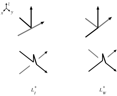
FIG. 13.: The non-planar intersections we consider. The top row are three dimensional views and the bottom row are the associated crossings that arise in the skein relations.

In order to compute the skein relations we consider a deformation of a straight-through planar intersection as shown in figure 14. The resulting integral is exactly the same as equation (31). The difference comes from the vector $\vec{u}$. That vector vanishes in the $z>0$ part of the loop. This implies that when one wants to rederive equation (32) one encounters ambiguities of the type $\delta(y)\Theta(y)$ exactly as when we deformed an $L_{W}$ intersection in a direction perpendicular to the plane. The way to handle this is again to introduce an indeterminate parameter $\alpha$. The resulting expression then reads, intersections with

FIG. 14.: The deformation of a straight through planar intersection into a crossing of the type $L^{+}_{I}$.

$$\int_{0}^{1}dt\delta_{\vec{u}}(t)<{\rm Tr}(H_{12}(\gamma)H_{34}(\gamma))>=-\alpha[{i\pi\over k}{\rm Tr}(H_{12}(\gamma)H_{34}(\gamma))-{2i\pi\over k}{\rm Tr}(H_{12}(\gamma)){\rm Tr}(H_{34}(\gamma))]$$ (49)

this can again be reinterpreted as,

$$\int_{0}^{1}dt\delta_{\vec{u}}(t)<W(L_{I})>=\alpha[{2i\pi\over k}<W(L_{W})>-{i\pi\over k}<W(L_{I})>].$$ (50)

In order to exponentiate, since the action mixes $L_{I}$ and $L_{W}$ we need to compute,

$$\left(\begin{array}[]{c}<W(L^{\mp}_{I})>\\ <W(L^{\mp}_{W})>\end{array}\right)=\exp\int_{0}^{1}dt\delta_{\pm{\vec{u}}}(t)\left(\begin{array}[]{c}<W(L_{I})>\\ <W(L_{W})>\end{array}\right)=\exp\left(\pm{i\pi\over k}\right)\left(\begin{array}[]{cc}-\alpha&2\alpha\\ \beta_{1}&\beta_{2}\end{array}\right)\left(\begin{array}[]{c}<W(L_{I})>\\ <W(L_{W})>\end{array}\right)$$ (51)

and one can show that in order to have consistency with the Mandelstam identity, $\beta_{1}=0$ $\beta_{2}=\alpha$. Notice that $\alpha$ is undetermined by the Mandelstam identities and we therefore have a one-parameter family of definitions of the skein relation for the crossing. Exponentiating explicitly and identifying the variable $k$ as before, we get,

$$<W(L^{\pm}_{I})> = q^{\mp{\alpha\over 4}}<W(L_{I})>+(q^{\pm{\alpha\over 4}}-q^{\mp{\alpha\over 4}})<W(L_{0})>$$ (52)

$$<W(L^{\pm}_{W})> = q^{\pm{\alpha\over 4}}<W(L_{0})>.$$ (53)

If $\alpha=0$ we get that $L^{\pm}_{I}\equiv L_{I}$ and $L^{\pm}_{W}\equiv L_{W}$, so the non-planar and planar intersections are treated in the same way.

It is also immediate to prove from the skein relations (52,45,46) that,

$$<W(L^{\pm}_{I})>|_{\alpha=1} = <W(L_{+})>$$ (54)

$$<W(L^{\pm}_{I})>|_{\alpha=0} = <W(L_{I})>$$ (55)

$$<W(L^{\pm}_{I})>|_{\alpha=-1} = <W(L_{-})>$$ (56)

so we see that for different values of the free parameter associated with the non-planar intersections we can have them play the same role as over-crossings, intersections and under-crossings. This highlights the relation between the value of the $\alpha$ parameter and the different types of regularizations it implies for the intersections.

As in the non-intersecting case, all the regular invariant information of the $<W(\gamma)>$ is concentrated in a multiplicative “phase factor”. One can divide by it and construct an ambient isotopic invariant, which for $SU(2)$ is the Jones polynomial. In the non-intersecting case, the writhe $w(\gamma)$ can be computed by evaluating the expectation value of a Wilson loop in a $U(1)$ Chern–Simons theory,

$$<W(\gamma)>|_{U(1)}=q^{w}(\gamma),$$ (57)

with skein relations,

$$w(\hat{L}_{\pm}) = \pm 1$$ (58)

$$w(L_{\pm}) = \pm 1$$ (59)

$$w(L_{I}) = w(L_{0})=0$$ (60)

$$w(L^{\pm}_{I}) = \pm\alpha$$ (61)

If one now defines a polynomial $J(\gamma)$ through

$$J(\gamma)={1\over 2}q^{-{3\over 4}w(\gamma)}<W(\gamma)>,$$ (62)

the result is ambient isotopic invariant.

The above definition of the Jones polynomial is also valid for multiloops, with a suitable generalization of the Abelian calculation of the writhe for multiloops. From the expression of the resulting Jones polynomial one can get an expression for the Gauss linking number of two loops with intersections. The resulting expression is consistent with lattice definitions of the linking number with intersections [26, 27].

E Triple and higher intersections

We will not discuss in detail the generalization to triple intersections in this paper, we sketch in this subsection how does one perform the generalization of the construction to that case. In the case of triple intersections, there are many types of possible independent vertices. In the case of planar intersections it is easy to see that one can deform them to double intersections, using the same techniques as for the $L_{W}$’s. For the case of non-planar triple intersections, there are 10 independent vertices. All of them can be related to double intersections through deformations similar to the one that connects $L_{I}$ with $L_{\pm}$. In order to exponentiate the infinitesimal deformations, one again has to exponentiate a matrix that connects the different intersection types. It will be a sparse $10\times 10$ matrix. Again regularization issues will leave many coefficients undetermined and one would restrict them using the Mandelstam identities. It is not clear if the resulting polynomial will be completely determined by the Mandelstam identities or if new free parameters will appear. As in the double case, the Mandelstam identities are non-local and there are now three different possible connectivities of intersections that are needed to implement the identities.

F Loops with multiple lines

Throughout this paper we have assumed we were dealing with loops that have each line traversed only one. If one would like the polynomial that is being derived to take values on the complete set of loops that is of interest in quantum gravity and gauge theories, one needs to consider the case of loops with multiply traversed section. This is also of importance if one is to view the integral of the exponential of the Chern–Simons form as a rigorous measure on the space of connections modulo gauge transformations. We present here a brief discussion of how could one consider double lines, but a complete description again requires further study.

Let us consider a loop $\gamma$ and study the Wilson loop along $\gamma^{2}\equiv\gamma\circ\gamma$. Consider a generic direction in space $\vec{w}$ such that the tangent vector to $\gamma$ is never parallel to $\vec{w}$. Consider an continuous infinitesimal displacement of all the points of $\gamma$ along $\vec{w}$ such that an arbitrary point on $\gamma$ is kept fixed (we will call this point the origin of the loop). This produces a second copy of $\gamma$. If one deforms back and forth along $\vec{w}$ in this way one ends up with two copies of $\gamma$ that are connected at the origin through an intersection of the type $L_{I}$, as shown in figure 15. Because this is a planar deformation, the value of the expectation value of the Wilson loop does not change. We have therefore reduced the problem of computing the expectation value for a loop traversed twice to the problem of computing the expectation value along a simply traversed loop with an intersection of one of the types studied before. It is worthwhile noticing that applying the Mandelstam identity (40) at the resulting intersection one gets the identity $<W(\gamma)W(\gamma)>=<W(\gamma\circ\gamma)>+2$.

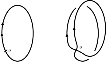
FIG. 15.: The deformation of a loop traversed twice into two loops with an intersection.

If one wants to consider a more general situation, in which a loop could have portions that are traversed twice, one can extend the above result in a relatively straightforward manner. Even if there are planar intersections of the multiply traversed segment with another segment one can separate them without additional contributions. However, if there are triple non-planar intersections involving sections multiply traversed, the deformation will give non-trivial contributions. These contributions can be evaluated explicitly given a specific loop.

V Conclusions

We have shown how to use variational techniques to obtain exact expressions for the knot invariant associated with the expectation value of the Wilson loop in Chern–Simons theory. The method is completely general in the sense that it can be used in Chern–Simons theory with any semisimple gauge group with small generalizations. We have worked out explicitly the value of the invariant not only for smooth loops but also for loops with double planar and non-planar intersections. The resulting invariant is compatible with the Mandelstam identities of the gauge group and therefore is suitable for providing invariants of interest as quantum states of topological field theories and quantum gravity. Having a well defined linear function on the space of loops compatible with the Mandelstam identities may allow also, using the techniques of Ashtekar and collaborators [28] to define in a rigorous way a measure in the space of connections modulo gauge transformations $d\mu(A)$. Such a measure would allow to give rigorous meaning in a mathematical sense to expression of the form $\int dAe^{kS_{CS}}f(A)$ for any gauge invariant function $f(A)$. The generalization of the work described in this paper to triple intersections is straightforward and relevant for quantum gravity applications. The possibility of computing explicitly the knot polynomials associated with Chern–Simons theory for any group is clearly of relevance in other physics applications, like the recent discovery of Chern–Simons states in supergravity has shown [18]. It is expected that these results will be extendible to $N>1$ supergravity where this method will provide with a simple method of characterizing the potentially new invariants that may arise.

A Commutativity of the $\delta$ operators

We wish to evaluate the successive action of two $\delta$ operators on $<W(\gamma)>$. We only discuss the case of a regular (non-intersecting) point of the loop. The first $\delta$ acts as indicated in (21), and using the Fierz identity we get,

$$\delta_{\vec{u}}(t)<W(\gamma)>=-{3\pi i\over k}\int_{0}^{1}ds\dot{\eta}^{a}(s,t){\eta^{\prime}}^{b}(s,t)\epsilon_{abc}\oint_{\gamma}dy^{c}\delta^{3}(\eta(s,t)-y)<W(\gamma)>.$$ (A1)

The second $\delta$ has two contributions, stemming from the action of the loop derivative on the loop dependence of $<W(\gamma)>$ and $\oint_{\gamma}$ respectively. The term that contributes to the commutator is the latter, since the contribution on the Wilson loop is the same in both orders. Let us therefore evaluate explicitly the non-trivial contribution,

$$[\delta(t_{1}),\delta(t_{2})] = -{3\pi i\over k}\int_{0}^{1}ds_{1}\int_{0}^{1}ds_{2}\dot{\eta}^{a}(s_{1},t_{1}){\eta^{\prime}}^{b}(s_{1},t_{1})\dot{\eta}^{c}(s_{2},t_{2}){\eta^{\prime}}^{d}(s_{2},t_{2})\epsilon_{ab[c}\partial_{d]}\delta^{3}(x-\eta(s_{1},t_{1}))|_{x=\eta(s_{2},t_{2})}$$ (A3)

$$-(t_{1}\leftrightarrow t_{2})$$

$$= -{3\pi i\over k}\int_{0}^{1}ds_{1}\int_{0}^{1}ds_{2}\dot{\eta}^{a}(s_{1},t_{1}){\eta^{\prime}}^{b}(s_{1},t_{1})\dot{\eta}^{c}(s_{2},t_{2})\epsilon_{abc}\partial_{s_{2}}\delta^{3}(\eta(s_{2},t_{2})-\eta(s_{1},t_{1}))$$ (A6)

$$+{3\pi i\over k}\int_{0}^{1}ds_{1}\int_{0}^{1}ds_{2}\dot{\eta}^{a}(s_{1},t_{1}){\eta^{\prime}}^{b}(s_{1},t_{1}){\eta^{\prime}}^{d}(s_{2},t_{2})\epsilon_{abd}\partial_{t_{2}}\delta^{3}(\eta(s_{2},t_{2})-\eta(s_{1},t_{1}))$$

$$-(t_{1}\leftrightarrow t_{2}).$$

One can now pick a coordinate chart in which $\delta^{3}(\eta(s_{2},t_{2})-\eta(s_{1},t_{1}))=Z\delta(s_{2}-s_{1})\delta(t_{2}-t_{1})$, where $Z$ is a regularization dependent factor that does not depend on $s_{2}$ or $t_{2}$. Using the distributional identity,

$$f(y)\partial_{y}\delta(y-x)=f(x)\partial_{y}\delta(y-x)-\delta(y-x)\partial_{x}f(x)$$ (A7)

it is immediate to check that the contributions vanish. The result is obviously dependent on a regularization choice.

REFERENCES

- [1] E. Witten, Commun. Math. Phys 121, 351 (1989).
- [2] L. Kauffman, “On knots”, Annals of Mathematics Studies, Princeton University Press, Princeton (1987).
- [3] J. Hoste, A. Ocneanu, K. Millet, P. Freyd, W. Lickorish, D. Yetter, Bull. Am. Math. Soc. 129, 239 (1985).
- [4] G. Moore, N. Seiberg, Phys. Lett. B212, 451 (1988).
- [5] L. Smolin, Mod. Phys. Lett. A4 1091 (1989).
- [6] P. Cotta-Ramusino, E. Guadagnini, M. Martellini, M. Mintchev Nuc. Phys. B330, 557 (1990).
- [7] Yu. M. Makeenko, A. A. Migdal, Phys. Lett. B88, 135 (1979); Nucl. Phys. B188, 269 (1981).
- [8] B. Brügmann, R. Gambini, J. Pullin, Nucl. Phys. B385, 587 (1992).
- [9] L. Kauffman, in “Knots and quantum gravity”, editor J. Baez, Oxford University Press, Oxford (1993).
- [10] R. Gambini, A. Trias, Nucl. Phys. B278, 436 (1986).
- [11] C. Rovelli, L. Smolin, Nucl. Phys. B331, 80 (1990).
- [12] A. Ashtekar, Phys. Rev. Lett. 57, 2244 (1986); Phys. Rev. D36, 1587 (1987).
- [13] C. Rovelli, L. Smolin, Phys. Rev. Lett. 61, 1155 (1988).
- [14] T. Jacobson, L. Smolin, Nucl. Phys. B299, 295 (1988).
- [15] B. Brügmann, J. Pullin, Nucl. Phys. B363, 221 (1991).
- [16] R. Gambini, J. Pullin “Loops, knots, gauge theories and quantum gravity”, Cambridge University Press (in press).
- [17] H. Kodama, Phys. Rev. D42, 2548 (1990).
- [18] D. Armand-Ugon, R. Gambini, O. Obregón, J. Pullin, Nucl. Phys. B460, 615 (1996).
- [19] L. Kauffman “Knots and physics”, World Scientific Series on Knots and Everything 1, World Scientific, Singapore (1991).
- [20] B. Brügmann, Int. J. Theor. Phys. 34, 145 (1995).
- [21] A. Ashtekar, J. Lewandowski, in “Knots and quantum gravity”, J. Baez editor, Oxford University Press, Oxford (1993).
- [22] I. Aref’eva, Theor. Math. Phys 43, 353 (1980) (Teor. Mat. Fiz. 43, 111 (1980)).
- [23] M. Awada, Comm. Math. Phys. 129, 329 (1990).
- [24] S. Major, L. Smolin, preprint gr-qc@xxx.lanl.gov:9512020 (1995).
- [25] D. Armand-Ugon, R. Gambini, P. Mora, Phys. Lett. B305, 214 (1993); Jour. Knot. Theor. Ramif. 4, 1 (1995).
- [26] A. Polikarpov, Moscow preprint ITEF-91-049 (1991).
- [27] H. Fort, R. Gambini, J. Pullin, in preparation.
- [28] A. Ashtekar, J. Lewandowski, D. Marolf, J. Mourao, T. Thiemann, “Quantization of diffeomorphism invariant theories of connections with local degrees of freedom”, preprint gr-qc@xxx.lanl.gov:9504018 (1995).