NSF-ITP-96-01

hep-th/9601038


Consistency Conditions for Orientifolds and D-Manifolds


Eric G. Gimon

Department of Physics

University of California Santa Barbara

Santa Barbara, CA  93106

e-mail: egimon@physics.ucsb.edu

Joseph Polchinski

Institute for Theoretical Physics

University of California

Santa Barbara, CA  93106-4030

e-mail: joep@itp.ucsb.edu


Abstract

We study superstrings with orientifold projections and with generalized open string boundary conditions (D-branes). We find two types of consistency condition, one related to the algebra of Chan-Paton factors and the other to cancellation of divergences. One consequence is that the Dirichlet 5-branes of the Type I theory carry a symplectic gauge group, as required by string duality. As another application we study the Type I theory on a $K3$ $Z_{2}$ orbifold, finding a family of consistent theories with various unitary and symplectic subgroups of $U(16)\times U(16)$. We argue that the $K3$ orbifold with spin connection embedded in gauge connection corresponds to an interacting conformal field theory in the Type I theory.

1 Introduction

One of the notable features of string duality has been the convergence of many previously disjoint lines of development. For example, certain once-obscure string backgrounds, namely orientifolds [1-3] and D-manifolds [3], have proven to be dual to more familiar backgrounds [4-8]. In order to find the nonperturbative structure underlying string duality it is important to understand as fully as possible all limits of the theory. The purpose of the present paper is to develop the consistency conditions for orientifolds and D-manifolds.

Orientifolds are generalized orbifolds. In the orbifold construction, discrete internal symmetries of the world-sheet theory are gauged. In the orientifold, products of internal symmetries with world-sheet parity reversal are also gauged. D-manifolds are manifolds with special submanifolds (D-branes) on which strings are allowed to end. These are labeled by a generalized Chan-Paton index, each value of which corresponds to restricting the string endpoint to a given submanifold of spacetime.

We will discuss consistency conditions of two types. The first comes from closure of the operator product expansion, which restricts the action of the discrete gauge symmetries on the Chan-Paton index. One consequence is that D 5-branes in Type I string theory must have a symplectic rather than orthogonal gauge projection: this is a world-sheet derivation of a result previously found from string duality [7]. Also, D 3-branes and 7-branes are inconsistent in the Type I superstring, while D 1-branes have an orthogonal gauge projection.

The second condition is cancellation of divergences and anomalies at one loop [9], which can be recast in terms of consistency of the field equations [10]. Here we focus on a simple example, the Type I theory on a K3 orbifold. We find all solutions to the consistency conditions, leading to gauge groups which are various unitary and symplectic subgroups of $U(16)\times U(16)$. Rather surprisingly, we do not find a solution with the spin connection embedded in the gauge connection. We argue that this theory, while it must exist, does not correspond to a free conformal field theory. Finally, we discuss various related work.

2 Orientifolds and Chan-Paton Factors

The orientifold group contains elements of two kinds. The first are purely internal symmetries $g$ of the world-sheet theory, forming a subgroup $G_{1}$. For the purposes of the present paper we will think of these as spacetime symmetries, though more generally (as in asymmetric orbifolds) one could consider symmetries whose spacetime interpretation is less clear. The second are elements of the form $\Omega h$, where $\Omega$ is the world-sheet parity transformation and $h$ is again a spacetime symmetry, now chosen from a set $G_{2}$. Closure implies that $\Omega h\Omega h^{\prime}\in G_{1}$ for $h,h^{\prime}\in G_{2}$, and if all elements of $G_{2}$ commute with $\Omega$ this is simply $G_{2}G_{2}=G_{1}$. The full orientifold group is $G=G_{1}+\Omega G_{2}$.

In the orientifold construction this group is gauged, meaning that one sums over all group elements around any nontrivial path on the world-sheet. This projects onto states invariant under $G_{1}$ and $\Omega G_{2}$. Elements of $G_{1}$ also lead to twisted closed strings, from a gauge transformation in going around a closed string. The factor $\Omega G_{2}$ means that orientation-reversal (combined with a $G_{2}$ action on the fields) is now part of the local symmetry group, so that unoriented world-sheets are included. The elements of $\Omega G_{2}$ do not give rise directly to new (twisted) sectors of the string Hilbert space; we will discuss later the extent to which it is useful to think of the open strings as being these twisted states.

The Chan-Paton index $i$ labels a set of a submanifolds (D-branes) $M_{i}$, with a string end-point in state $i$ constrained to lie on $M_{i}$. Some of the $M_{i}$ may be coincident. Each element of the discrete gauge group will have some action on the Chan-Paton index. Denote a general open string state by $|\psi,ij\rangle$, where $\psi$ is the state of the world-sheet fields and $i$ and $j$ are the Chan-Paton states of the left and right endpoints; the boundary conditions on the fields in $\psi$ are of course $i,j$-dependent. The elements $g$ act on this as

$$g:\qquad|\psi,ij\rangle\ \to\ (\gamma_{g})_{ii^{\prime}}|g\cdot\psi,i^{\prime}j^{\prime}\rangle(\gamma_{g}^{-1})_{j^{\prime}j}.$$ (2.1)

for some matrix $\gamma_{g}$ associated with $g$.111Some time after the completion of this paper, we learned that much of the following formalism was developed for $Z_{2}$ orientifolds of the bosonic string by Pradisi and Sagnotti in the early paper [11]. This form is determined by the requirement that a general trace of products of wavefunctions be invariant. The action on the Chan-Paton factors must also be consistent with the action on the fields. That is, for each D-brane $M_{i}$, the spacetime-transformed D-brane $g\cdot M_{i}$ must appear, and the only nonzero elements of $\gamma_{g}$ are those connecting $M_{i}$ and $g\cdot M_{i}$. If $M_{i}$ is left fixed by $g$ then diagonal elements are allowed. Similarly,

$$\Omega h:\qquad|\psi,ij\rangle\ \to\ (\gamma_{\Omega h})_{ii^{\prime}}|\Omega h\cdot\psi,j^{\prime}i^{\prime}\rangle(\gamma_{\Omega h}^{-1})_{j^{\prime}j}.$$ (2.2)

Note that the orientation reversal transposes the two endpoints. The $\gamma_{g}$ and $\gamma_{\Omega h}$ are unitary.

To derive further constraints on the matrices $\gamma_{g}$ and $\gamma_{\Omega h}$, let us first demonstrate that the discrete gauge group may not include pure gauge twists, those with $g=1\in G_{1}$ with $\gamma_{1}$ nontrivial. The point is that the allowed Chan-Paton wavefunctions must form a complete set: the set of string wavefunctions $|\psi,ij\rangle$ must include nontrivial states for all pairs $ij$. One can see this heuristically by noting that if there are states $ik$ and $jl$ for some $k$ and $l$ (and therefore also $lj$ by CPT), then by a splitting-joining interaction one obtains also $ij$ and $lk$. This interaction occurs in the interior of the string and so by locality cannot depend on the values of the endpoints. One can make this precise by requiring that the annulus factorize correctly on the closed string poles, so this is actually a one-loop conditionβ€”at tree-level it would be consistent to truncate to block-diagonal wavefunctions. Now, if the identity appears in $G_{1}$, we have the projection

$$|\psi,ij\rangle\ =(\gamma_{1})_{ii^{\prime}}|\psi,i^{\prime}j^{\prime}\rangle(\gamma_{1}^{-1})_{j^{\prime}j}.$$ (2.3)

Since this holds for a complete set, Schur’s lemma implies that $\gamma_{1}\propto 1$; we may as well set $\gamma_{1}=1$ because the overall phase is irrelevant.

This implies a further restriction on the $\gamma_{g}$ and $\gamma_{\Omega h}$: they must satisfy the algebra of the corresponding symmetries, up to a phase. For example, $\gamma_{g_{1}}\gamma_{g_{2}}\gamma_{g_{2}^{-1}g_{1}^{-1}}\propto 1$, else we would contradict the result in the previous section. As another example, suppose that $G_{1}$ includes an element of order 2, $g^{2}=1$. Then on a string state,

$$g^{2}:\qquad|\psi,ij\rangle\ \to\ (\gamma_{g}^{2})_{ii^{\prime}}|\psi,i^{\prime}j^{\prime}\rangle(\gamma_{g}^{-2})_{j^{\prime}j},$$ (2.4)

and so (by choice of phase)

$$\gamma_{g}^{2}=1.$$ (2.5)

Similarly, if $G_{2}$ includes an element of order 2, then $(\Omega h)^{2}$ acts as

$$(\Omega h)^{2}:\qquad|\psi,ij\rangle\ \to\ (\gamma_{\Omega h}(\gamma_{\Omega h}^{T})^{-1})_{ii^{\prime}}|\psi,i^{\prime}j^{\prime}\rangle(\gamma_{\Omega h}^{T}\gamma_{\Omega h}^{-1})_{j^{\prime}j},$$ (2.6)

implying that

$$\gamma_{\Omega h}^{T}=\pm\gamma_{\Omega h}.$$ (2.7)

Let us apply this to the Type I theory. The Type I theory is an orientifold of the Type IIB theory with the single nontrivial element $\Omega$; that is, $h=h^{2}=1$. Tadpole cancellation, to be reviewed in the next section, requires that the orientifolding be accompanied by the inclusion of $n$ 9-branes, corresponding to purely Neumann boundary conditions. If $\gamma_{\Omega}$ is symmetric, we can choose a basis such that $\gamma_{\Omega}=I$. If $\gamma_{\Omega}$ is antisymmetric, we can choose a basis such that $\gamma_{\Omega}$ is the symplectic matrix

$$M=\left[\begin{array}[]{cc}0&iI\\ -iI&0\end{array}\right],$$ (2.8)

where $n$ must be even. For the massless open string vector, the $\Omega$ eigenvalue of the oscillator state is $-1$. For $\gamma_{\Omega}$ symmetric, the Chan-Paton wavefunction of the vector is then antisymmetric, giving the gauge group $SO(n)$. For $\gamma_{\Omega}$ antisymmetric, the massless vectors form the adjoint of $USp(n)$. Tadpole cancellation requires $SO(32)$.

Now let us consider adding 5-branes. The Chan-Paton index runs over both 9-branes and 5-branes. The only freedom in eq. (2.7) is the overall sign. Since we are required to take the $SO$ projection on the 9-branes it appears that we are required to take the same projection on the 5-branes. This is in contradiction with ref. [7], where it was found that string duality requires a symplectic gauge group on the Type I 5-brane. To understand this we need to be somewhat more careful.

The point is that, although $\Omega^{2}$ acts trivially on the world-sheet fields, it may be a nontrivial phase in various sectors of the Hilbert space. The phase of $\Omega$ is determined by the requirement that it be conserved by the operator product of the corresponding vertex operators. Thus, the massless vector state, with vertex operator $\partial_{t}X^{\mu}$, necessarily has $\Omega=-1$ because $\Omega$ changes the orientation of the tangent derivative $\partial_{t}$; we have used this fact two paragraphs previously. In the 55 sector (that is, strings with both ends on a 5-brane), for the massless vertex operator is $\partial_{t}X^{\mu}$ ($\Omega=-1$) for $\mu$ parallel to the 5-brane, and $\partial_{n}X^{\mu}$ ($\Omega=+1$) for $\mu$ perpendicular. On these states, $\Omega^{2}=1$, and the same is true for the rest of the 99 and 55 Hilbert spaces. To see this, use the fact that $\Omega$ multiplies any mode operator $\psi_{r}$ by $\pm e^{i\pi r}$. (Details of the mode expansions are given in section 3.3.) In the Neveu-Schwarz sector this is $\pm i$, but the GSO projection requires that these modes operators act in pairs.222The OPE is single-valued only for GSO-projected vertex operators. So $\Omega=\pm 1$, and this holds in the R sector as well by supersymmetry.

Now consider the Neveu-Schwarz 59 sector. The four $X^{\mu}$ with mixed Neumann-Dirichlet boundary conditions, say $\mu=6,7,8,9$, have a half-integer mode expansion. Their superconformal partners $\psi^{\mu}$ then have an integer mode expansion and the ground state is a representation of the corresponding Clifford algebra. The vertex operator is thus a spin field: the periodic $\psi^{\mu}$ contribute a factor $V=e^{i(H_{3}+H_{4})/2}$, where $H_{3,4}$ are from the bosonization of the four periodic $\psi^{6,7,8,9}$ [12]. We need only consider this part of the vertex operator, as the rest is the same as in the 99 string and so has $\Omega^{2}=+1$. Now, the operator product of $V$ with itself (which is in the 55 or 99 sector) involves $e^{i(H_{3}+H_{4})}$, which is the bosonization of $(\psi^{6}+i\psi^{7})(\psi^{8}+i\psi^{9})$. This in turn is the vertex operator for the state $(\psi^{6}+i\psi^{7})_{-1/2}(\psi^{8}+i\psi^{9})_{-1/2}|0\rangle$. Finally we can deduce the $\Omega$ eigenvalue. For $|0\rangle$ it is $+1$, because its vertex operator is the identity, while each $\psi_{-1/2}$ contributes either $-i$ (for a 99 string) or $+i$ (for a 55 string), for an overall $-1$. That is, the $\Omega$ eigenvalue of $V\cdot V$ is $-1$, so therefore is the $\Omega^{2}$ eigenvalue of $V$.

Returning to eq. (2.6), in the 59 sector there is an extra $-1$ from the above argument. Separate $\gamma_{\Omega}$ into a block $\gamma_{\Omega,9}$ which acts on the 9-branes and a block $\gamma_{\Omega,5}$ which acts on the 5-branes. We have $\gamma_{\Omega,9}^{T}=+\gamma_{\Omega,9}$ from tadpole cancellation. To cancel the sign in the 59 sector we then need $\gamma_{\Omega,5}^{T}=-\gamma_{\Omega,5}$, giving symplectic groups on the 5-brane as found in ref. [7]. This argument seems roundabout, but it is faithful to the logic that the actions of $\Omega$ in the 55 and 99 sectors are related because they are both contained in the 59 $\cdot$ 95 product. Further, there does not appear to be any arbitrariness in the result.

Let us briefly review the consequences of this projection [7]. Consider a pair of coincident 5-branes, since the symplectic projection requires an even number. The world-brane vectors $\partial_{t}X^{\mu}$ ($\mu$ parallel to the 5-brane) have Chan-Paton wavefunctions $\sigma^{a}_{ij}$, gauge group $USp(2)=SU(2)$. The world-brane scalars $\partial_{n}X^{\mu}$ ($\mu$ perpendicular to the 5-brane) have Chan-Paton wavefunction $\delta_{ij}$. Since these are the collective coordinates for 5-branes [3], the wavefunction $\delta_{ij}$ means that the two 5-branes move together as a unit. The need for this can also be seen in another way [13]. In the Type I theory the force between 5-branes, and between 1-branes, is half of that calculated in ref. [5] because of the orientation projection. The product of the charges of a single 1-brane and single 5-brane would then be only half a Dirac-Teitelboim-Nepomechie unit; but since the 5-branes are always paired the quantization condition is respected.

The IIB theory also contains $p=1$, 3, and 7-branes. The above argument gives $\Omega^{2}=(\pm i)^{(9-p)/2}$. This requires an $SO$ projection on the 1-brane, consistent with Type I-heterotic duality. On the 3- and 7-branes it leads to an inconsistency. This is a satisfying result, as there is no conserved charge in the Type I theory to give rise to such $p$-branes.

We do not know that we have found the complete set of consistency conditions of this type, but no others are evident to us.

3 Tadpoles

Modular invariance on the torus is one of the central consistency requirements for closed oriented strings. For open and unoriented one-loop graphs there is no corresponding modular group, but cancellation of divergences plays an analogous role in constraining the theory [9]. In refs. [14, 10] these divergences were obtained in the ten-dimensional Type I theory from one-loop vacuum amplitudes. In ref. [10] they were reinterpreted in terms of an inconsistency in the field equation for a Ramond-Ramond (RR) 10-form potential. It is useful to recall the latter interpretation, now generalized to all RR forms. D-branes and orientifold fixed-planes are electric and magnetic sources for the RR fields [5]. The $n$-form field strength $H_{n}$ thus satisfies

$$dH_{n}=*J_{9-n},\qquad d*H_{n}=*J_{n-1}$$ (3.1)

where $J_{9-n}$ and $J_{n-1}$ are sources of the indicated rank. The field equations are consistent only if

$$\int_{C_{k}}*J_{10-k}=0$$ (3.2)

for all closed curves $C_{k}$. In flat $d=10$ the only nontrivial closed curves are the points $C_{0}$, and the corresponding constraint on $J_{10}$ requires the gauge group $SO(32)$. In a compact theory there will be more constraints.

More generally, the right-hand side of the field equations (3.1) will include additional terms from Chern-Simons couplings of the RR fields to curvature and gauge field strengths. In the present work we consider only orientifolds of flat backgrounds, but the more general case will also be interesting.

The tadpole constraints were applied to orientifolds in refs. [2, 16, 17, 18]. Many of the results in the present section can be found in ref. [2], except that our treatment of the Chan-Paton factors will be more general.

3.1 General Framework

The divergences can be determined from the vacuum amplitudes on the Klein bottle (KB), MΓΆbius strip (MS), and cylinder (C). In fig. 1 these surfaces are all depicted as cylinders of length $2\pi l$ and circumference $2\pi$, with the ends being either boundaries or crosscaps.
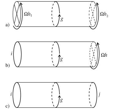
Refer to caption
Figure 1: Riemann surfaces described by eq. (3.3). a) Klein bottle. b) MΓΆbius strip. c) Cylinder.

Taking coordinates $0\leq\sigma^{1}\leq 2\pi l$, $0\leq\sigma^{2}\leq 2\pi$, the periodicity and boundary conditions on generic world-sheet fields $\phi$ (and their derivatives) are as follows:

KB: $\displaystyle\phi(0,\pi+\sigma^{2})=\Omega\tilde{h}_{1}\phi(0,\sigma^{2}),\quad\phi(2\pi l,\pi+\sigma^{2})=\Omega\tilde{h}_{2}\phi(2\pi l,\sigma^{2})$
$\displaystyle\phi(\sigma^{1},2\pi+\sigma^{2})=\tilde{g}\phi(\sigma^{1},\sigma^{2})$
MS: $\displaystyle\phi(0,\sigma^{2})\in\tilde{M}_{i},\quad\phi(2\pi l,\pi+\sigma^{2})=\Omega\tilde{h}\phi(2\pi l,\sigma^{2})$
$\displaystyle\phi(\sigma^{1},2\pi+\sigma^{2})=\tilde{g}\phi(\sigma^{1},\sigma^{2})$
C: $\displaystyle\phi(0,\sigma^{2})\in\tilde{M}_{i},\quad\phi(2\pi,\sigma^{2})\in\tilde{M}_{j},$ (3.3)
$\displaystyle\phi(\sigma^{1},2\pi+\sigma^{2})=\tilde{g}\phi(\sigma^{1},\sigma^{2}).$

It is convenient to include in the periodicity or boundary conditions $g$, $h$, and $M_{i}$, besides the spacetime part discussed earlier, a $\pm 1$ on the world-sheet fermions from the GSO projection; the tilde is a reminder of this additional information. The respective definitions (3.3) are consistent only if

KB: $\displaystyle(\Omega\tilde{h}_{1})^{2}=(\Omega\tilde{h}_{2})^{2}=\tilde{g}$
MS: $\displaystyle(\Omega\tilde{h})^{2}=\tilde{g},\quad\tilde{g}\tilde{M}_{i}=\tilde{M}_{i}$
C: $\displaystyle\tilde{g}\tilde{M}_{i}=\tilde{M}_{i},\quad\tilde{g}\tilde{M}_{j}=\tilde{M}_{j}\ ;$ (3.4)

else the corresponding path integral vanishes.

These graphs will have divergences from the tadpoles shown in fig. 2.
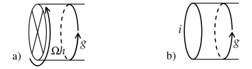
Refer to caption
Figure 2: Tadpoles in the $g$-twisted sector. a) Crosscap: fields at opposite points differ by an $\Omega h$ transformation, where $g=(\Omega h)^{2}$. b) Boundary in state $i$. The manifold $M_{i}$ must be fixed under $g$.

If there are $m$ non-compact dimensions, the dangerous tadpoles will be from those massless RR states which are $m$-forms in the non-compact directions. In general there are several such tadpoles, coming from twisted and untwisted sectors.

To write the Klein bottle and MΓΆbius strips in terms of traces, take the alternate coordinate region $0\leq\sigma^{1}\leq 4\pi l$, $0\leq\sigma^{2}\leq\pi$ with periodicities333This is done by taking the upper strip $\pi\leq\sigma^{2}\leq 2\pi$, inverting it from right to left and multiplying the fields by $(\Omega\tilde{h}_{2})^{-1}$, and gluing it to the right side of the lower strip: with this construction the fields are smooth at $\sigma^{1}=2\pi l$.

KB: $\displaystyle\phi(\sigma^{1},\pi+\sigma^{2})=\Omega\tilde{h}_{2}\phi(4\pi l-\sigma^{1},\sigma^{2}),\quad\phi(4\pi l,\sigma^{2})=\tilde{g}^{\prime}\phi(0,\sigma^{2})$
MS: $\displaystyle\phi(\sigma^{1},\pi+\sigma^{2})=\Omega\tilde{h}\phi(4\pi l-\sigma^{1},\sigma^{2}),\quad\phi(0,\sigma^{2})\in\tilde{M}_{i},$ (3.5)
$\displaystyle\qquad\qquad\phi(4\pi l,\sigma^{2})\in\tilde{M}_{i}$

where $\tilde{g}^{\prime}=\Omega\tilde{h}_{2}(\Omega\tilde{h}_{1})^{-1}$. Rescaling the coordinates to standard length ($\pi$ for open strings and $2\pi$ for closed), the respective amplitudes are

KB: $\displaystyle{\rm Tr}_{{\rm c},g^{\prime}}\left(\Omega\tilde{h}_{2}(-1)^{F+\tilde{F}}e^{\pi(L_{0}+\tilde{L}_{0})/2l}\right)$
MS: $\displaystyle{\rm Tr}_{{\rm o},ii}\left(\Omega\tilde{h}(-1)^{F}e^{\pi L_{0}/4l}\right)$
C: $\displaystyle{\rm Tr}_{{\rm o},ij}\left(\tilde{g}(-1)^{F}e^{\pi L_{0}/l}\right)$ (3.6)

The closed string trace is labeled by the spacelike twist $g^{\prime}$ and the open string traces are labeled by the Chan-Paton states.

The full one-loop amplitude is

$$\int_{0}^{\infty}\frac{dt}{2t}\left\{{\rm Tr}_{{\rm c}}\left({\bf P}(-1)^{\bf F}e^{-2\pi t(L_{0}+\tilde{L}_{0})}\right)+{\rm Tr}_{{\rm o}}\left({\bf P}(-1)^{\bf F}e^{-2\pi tL_{0}}\right)\right\},$$ (3.7)

where P includes the GSO and $G$-projections, and F is the spacetime fermion number. The traces are over the transverse oscillator states and include a spacetime momentum sum. The sums in the projection operators and over twisted sectors and Chan-Paton states are equivalent to summing the surfaces in fig. 1 over all tadpole types. Evaluating the traces, the $t\to 0$ limit produces the divergences of interest. Note that the loop modulus $t$ is related to the cylinder length $l$ differently for each surface,

$$\mbox{KB:}\ \ t=\frac{1}{4l},\qquad\mbox{MS:}\ \ t=\frac{1}{8l},\qquad\mbox{C:}\ \ t=\frac{1}{2l}.$$ (3.8)

3.2 Type I Theory on a $K3$ Orbifold

We will evaluate the tadpoles and solve the consistency conditions for one particular example. This is the Type I theory on a K3 $Z_{2}$ orbifold. The Type I theory includes a projection on $\Omega$. The orbifold is formed from the theory on a torus by projecting with $R_{6789}$, reflection of $X^{6,7,8,9}$; we will abbreviate this as $R$. Closure gives also the element $\Omega R$. To define $R$ we have to make a specific choice of its action on the fermions; we choose $R=e^{i\pi(J_{67}+J_{89})}$.

This example is of interest for a number of reasons. It is related by $T$-duality to many similar theories. A $T$-duality transformation on $X^{\mu}$ for given $\mu$ (abbreviated $T_{\mu}$) is a spacetime reflection, but only on the world-sheet right-movers. It transforms $\Omega$ to $\Omega R_{\mu}$ [3, 15]. Thus, $T_{6}$-duality takes the above orientifold group to $\{1,R_{6789},\Omega R_{6},\Omega R_{789}\}$, $T_{4567}$-duality takes it to $\{1,R_{6789},\Omega R_{4567},\Omega R_{4589}\}$, and so on. This is the simplest orientifold that is not just the $T$-dual of a toroidal theory.

We can anticipate some of the tadpole calculation. The $\Omega$ projection will require 9-branes as in the non-compact case [10]. Similarly the $\Omega R$ projection, being $T_{6789}$-dual to $\Omega$, will require 5-branes with fixed $X^{6,7,8,9}$. There is also the possibility of twisted sector tadpoles, and these will indeed appear. In all there are three tadpole types, the 10-form, 6-form, and twisted-sector 6-form (actually 16 of these last, one for each fixed point) and each receives two contributions. The 10-form receives contributions from the crosscap with $h=1$ and the 9-brane boundary with $g=1$, the 6-form from the crosscap with $h=R$ and the 5-brane boundary with $g=1$, and the twisted-sector 6-forms from 5-brane and 9-brane boundaries with $g=R$.

The IIB theory has $d=10,N=2\to d=6,N=4$ spacetime supersymmetry. The $\Omega$ projection leaves only the sum of the left- and right-moving supersymmetries, $Q_{\alpha}+\tilde{Q}_{\alpha}$. Similarly the $\Omega R$ projection leaves the linear combinations $Q_{\alpha}+R\tilde{Q}_{\alpha}$. The supersymmetries unbroken by both projections correspond to the $+1$ eigenvalues of $R$; this is half the eigenvalues of $R$ or a quarter of the original supersymmetries, $d=6,N=1$.

Let us work out the massless spectrum of this theory. We focus on the bosons, since the fermions will have the same partition function by supersymmetry. The massless spectrum for the right- or left-moving half of the closed string is

$$\begin{array}[]{rlcc}\mbox{Sector$\qquad$}&&R&SO(4)\mbox{ rep.}\\[4.0pt] \mbox{Untwisted NS:\ \ }&\psi_{-1/2}^{\mu}|0\rangle&+&({\bf 2},{\bf 2})\\ &\psi_{-1/2}^{m}|0\rangle&-&4({\bf 1},{\bf 1})\\ \mbox{R:\ \ }&|s_{1}s_{2}s_{3}s_{4}\rangle&&\\ &\quad s_{1}=+s_{2},\ s_{3}=-s_{4}&+&2({\bf 2},{\bf 1})\\ &\quad s_{1}=-s_{2},\ s_{3}=+s_{4}&-&2({\bf 1},{\bf 2})\\ \mbox{Twisted NS:\ \ }&|s_{3}s_{4}\rangle,\ s_{3}=-s_{4}&+&2({\bf 1},{\bf 1})\\ \mbox{R:\ \ }&|s_{1}s_{2}\rangle,\ s_{1}=-s_{2}&+&({\bf 1},{\bf 2})\\ \end{array}$$ (3.9)

Here, $\mu\in 2,3,4,5$, $m\in 6,7,8,9$, and $SO(4)=SU(2)\times SU(2)$ is the massless little group in 6 dimensions. We have imposed the GSO projection: all states listed have $(-1)^{F}=(-1)^{\tilde{F}}=1$. This is most easily determined by requiring that the vertex operators be local with respect to the supercharge $e^{-\phi/2}e^{i(H_{0}+H_{1}+H_{2}+H_{3}-H_{4})/2}$ (the minus sign in the exponent is necessary because this must have $R=+$); the ghost times longitudinal part contributes a net $Z_{2}$ branch cut in the NS sector and none in the R sector. The bosonic spectrum is given by the product a left-moving state with a right-moving state from the same sector and with the same $R$. In the NSNS sectors this is symmetrized by the $\Omega$ projection, and in the RR sectors it is antisymmetrized because each side is a fermion. Thus, including the degeneracy from the 16 fixed points, the massless closed string spectrum is

$$\begin{array}[]{rc}\mbox{Sector$\qquad$}&SO(4)\mbox{ rep.}\\[4.0pt] \mbox{Untwisted NSNS: }&({\bf 3},{\bf 3})+11({\bf 1},{\bf 1})\\ \mbox{RR: }&({\bf 3},{\bf 1})+({\bf 1},{\bf 3})+6({\bf 1},{\bf 1})\\ \mbox{Twisted NSNS: }&48({\bf 1},{\bf 1})\\ \mbox{RR: }&16({\bf 1},{\bf 1})\\ \end{array}$$ (3.10)

This is the $d=6$, $N=1$ supergravity multiplet, plus one tensor multiplet, plus 20 $({\bf 1},{\bf 1})$ hypermultiplets.

For the open strings consider first the 99 states, with massless bosonic (NS) spectrum

$$\begin{array}[]{lllc}&R=+&\Omega=+&SO(4)\mbox{ rep.}\\[4.0pt] \psi_{-1/2}^{\mu}|0,ij\rangle\lambda_{ji}&\lambda=\gamma_{R,9}\lambda\gamma_{R,9}^{-1}&\lambda=-\gamma_{\Omega,9}\lambda^{T}\gamma_{\Omega,9}^{-1}&({\bf 2},{\bf 2})\\ \psi_{-1/2}^{m}|0,ij\rangle\lambda_{ji}&\lambda=-\gamma_{R,9}\lambda\gamma_{R,9}^{-1}&\lambda=-\gamma_{\Omega,9}\lambda^{T}\gamma_{\Omega,9}^{-1}&4({\bf 1},{\bf 1}).\\ \end{array}$$ (3.11)

We have indicated the conditions imposed by the $R$ and $\Omega$ projections on the Chan-Paton wavefunctions $\lambda$. The subscript $9$ indicates the block of $\gamma_{R}$ or $\gamma_{\Omega}$ which acts on the 9-branes. For the 55 open strings, let us first consider $n_{I}$ 5-branes at the $I$’th fixed point of $R$. The massless spectrum is

$$\begin{array}[]{lllc}&R=+&\Omega=+&SO(4)\mbox{ rep.}\\[4.0pt] \psi_{-1/2}^{\mu}|0,ij\rangle\lambda_{ji}&\lambda=\gamma_{R,I}\lambda\gamma_{R,I}^{-1}&\lambda=-\gamma_{\Omega,I}\lambda^{T}\gamma_{\Omega,I}^{-1}&({\bf 2},{\bf 2})\\ \psi_{-1/2}^{m}|0,ij\rangle\lambda_{ji}&\lambda=-\gamma_{R,I}\lambda\gamma_{R,I}^{-1}&\lambda=\gamma_{\Omega,I}\lambda^{T}\gamma_{\Omega,I}^{-1}&4({\bf 1},{\bf 1}),\\ \end{array}$$ (3.12)

where now $\gamma_{R,I}$ and $\gamma_{\Omega,I}$ are the blocks acting on this set of 5-branes. The extra sign in the $\Omega$ projection follows from the form of the vertex operator, as discussed earlier. Now consider $n^{\prime}_{J}$ 5-branes at a non-fixed point $X$, which requires also $n^{\prime}_{J}$ at $-X$. The massless bosonic strings with both ends at $X$ are

$$\begin{array}[]{llc}&\Omega=+&SO(4)\mbox{ rep.}\\[4.0pt] \psi_{-1/2}^{\mu}|0,ij\rangle\lambda_{ji}&\lambda=-\gamma^{\prime}_{\Omega,J}\lambda^{T}\gamma^{\prime-1}_{\Omega,J}&({\bf 2},{\bf 2})\\ \psi_{-1/2}^{m}|0,ij\rangle\lambda_{ji}&\lambda=\gamma^{\prime}_{\Omega,J}\lambda^{T}\gamma^{\prime-1}_{\Omega,J}&4({\bf 1},{\bf 1}).\\ \end{array}$$ (3.13)

The $R$ projection relates these wavefunctions to those of the strings with ends at $-X$, but does not otherwise constrain them. For the 59 strings, we have in the two cases above

$$\begin{array}[]{llc}&R=+&SO(4)\mbox{ rep.}\\[4.0pt] |s_{3}s_{4},ij\rangle\lambda_{ji},\ s_{3}=-s_{4}&\lambda=\gamma_{R,I}\lambda\gamma_{R,9}^{-1}&2({\bf 1},{\bf 1})\\ \end{array}$$ (3.14)

and

$$\begin{array}[]{lc}&SO(4)\mbox{ rep.}\\[4.0pt] |s_{3}s_{4},ij\rangle\lambda_{ji},\ s_{3}=-s_{4}&2({\bf 1},{\bf 1}).\\ \end{array}$$ (3.15)

The $\Omega$ projection does not constrain these but determines the 95 state in terms of the 59 states.

3.3 Tadpole Calculation

We may now evaluate the sums (3.6) over the closed and open string spectra. The amplitudes are $\int_{0}^{\infty}dt/2t$ times

KB: $\displaystyle{\rm Tr}_{\rm NSNS+RR}^{\rm U+T}\left\{\frac{\Omega}{2}\,\frac{1+R}{2}\,\frac{1+(-1)^{F}}{2}e^{-2\pi t(L_{0}+\tilde{L}_{0})}\right\}$
MS: $\displaystyle{\rm Tr}_{\rm NS-R}^{99+55}\left\{\frac{\Omega}{2}\,\frac{1+R}{2}\,\frac{1+(-1)^{F}}{2}e^{-2\pi tL_{0}}\right\}$
C: $\displaystyle{\rm Tr}_{\rm NS-R}^{99+95+59+55}\left\{\frac{1}{2}\,\frac{1+R}{2}\,\frac{1+(-1)^{F}}{2}e^{-2\pi tL_{0}}\right\}.$ (3.16)

Here U (T) refers to the untwisted (twisted) closed string sector. On the Klein bottle we omit the $\frac{1}{2}(1+(-1)^{\tilde{F}})$ projector because the left- and right-moving states are identical in the trace. The open-string traces include a sum over Chan-Paton states.

The signs of the operators appearing in the traces, in the various sectors, were given implicitly in the previous section. For completeness we give the action of $\Omega$ on the various mode operators; the action of $R$ is obvious. In the closed string,

$$\Omega\alpha_{r}\Omega^{-1}=\tilde{\alpha}_{r},\qquad\Omega\psi_{r}\Omega^{-1}=\tilde{\psi}_{r},\qquad\Omega\tilde{\psi}_{r}\Omega^{-1}=-\psi_{r}$$ (3.17)

for integer and half-integer $r$. The minus sign is included in the last equation to give the convenient result $\Omega\psi_{M}\tilde{\psi}_{M}\Omega^{-1}=\psi_{M}\tilde{\psi}_{M}$ for any product $\psi_{M}$ of mode operators. Alternately this sign can be omitted: this just corresponds to $\Omega\to(-1)^{F}\Omega$, which has the same action on physical states. In open string, the mode expansions are

X​(Οƒ,0)=x+i​α′2β€‹βˆ‘m=βˆ’βˆžmβ‰ 0∞αmm​(ei​m​σ±eβˆ’i​m​σ)π‘‹πœŽ0π‘₯𝑖superscript𝛼′2superscriptsubscriptFRACOPπ‘šπ‘š0subscriptπ›Όπ‘šπ‘šplus-or-minussuperscriptπ‘’π‘–π‘šπœŽsuperscriptπ‘’π‘–π‘šπœŽX(\sigma,0)=x+i\sqrt{\frac{\alpha^{\prime}}{2}}\sum_{{m={-\infty}}\atop{m\neq 0}}^{\infty}\frac{\alpha_{m}}{m}(e^{im\sigma}\pm e^{-im\sigma}) (3.18)

with the upper sign for NN boundaries conditions and lower for DD (N=Neumann, D=Dirichlet). World-sheet parity, $X(\sigma,0)\to X(\pi-\sigma,0)$, takes

$$\alpha_{m}\to\pm e^{i\pi m}\alpha_{m}.$$ (3.19)

There is no corresponding result for the ND sector, since $\Omega$ takes this into a different, DN, sector. For fermions, the mode expansions are

$$\psi(\sigma,0)=\sum_{r}e^{ir\sigma}\psi_{r},\qquad\tilde{\psi}(\sigma,0)=\sum_{r}e^{-ir\sigma}\psi_{r}.$$ (3.20)

Parity, $\psi(\sigma,0)\to\pm\tilde{\psi}(\pi-\sigma,0)$, takes

$$\psi_{r}\to\pm e^{i\pi r}\psi_{r}$$ (3.21)

for integer and half-integer $r$. As in the closed string there is some physically irrelevant sign freedom. In evaluating the traces, note that $\Omega$ and $R$ act on the compact momenta $p^{m}$ and windings $\delta X^{m}=X^{m}(2\pi)-X^{m}(0)$ of the closed string as

$\displaystyle\Omega p^{m}\Omega^{-1}=p^{m},\qquad Rp^{m}R^{-1}=-p^{m}$
$\displaystyle\Omega\delta X^{m}\Omega^{-1}=-\delta X^{m},\qquad R\delta X^{m}R^{-1}=-\delta X^{m}$ (3.22)

and that only diagonal elements contribute in the traces. Similarly in the open string 99 sector there is an internal momentum, while in the 55 sector with fixed endpoints there is a winding $\delta X^{m}=X^{m}(\pi)-X^{m}(0)$.

It is useful to define444The $\sqrt{2}$ in $f_{2}$ corrects a typographical error in ref. [10].

$\displaystyle f_{1}(q)=q^{1/12}\prod_{n=1}^{\infty}\left(1-q^{2n}\right),\qquad f_{2}(q)=q^{1/12}\sqrt{2}\,\prod_{n=1}^{\infty}\left(1+q^{2n}\right)$
$\displaystyle f_{3}(q)=q^{-1/24}\prod_{n=1}^{\infty}\left(1+q^{2n-1}\right),\qquad f_{4}(q)=q^{-1/24}\prod_{n=1}^{\infty}\left(1-q^{2n-1}\right).$ (3.23)

These functions satisfy the β€˜abstruse identity’

$\displaystyle f_{3}^{8}(q)=f_{2}^{8}(q)+f_{4}^{8}(q)$ (3.24)

and have the modular transformations

f1​(eβˆ’Ο€/s)=s​f1​(eβˆ’Ο€β€‹s),f3​(eβˆ’Ο€/s)=f3​(eβˆ’Ο€β€‹s),f2​(eβˆ’Ο€/s)=f4​(eβˆ’Ο€β€‹s).formulae-sequencesubscript𝑓1superscriptπ‘’πœ‹π‘ π‘ subscript𝑓1superscriptπ‘’πœ‹π‘ formulae-sequencesubscript𝑓3superscriptπ‘’πœ‹π‘ subscript𝑓3superscriptπ‘’πœ‹π‘ subscript𝑓2superscriptπ‘’πœ‹π‘ subscript𝑓4superscriptπ‘’πœ‹π‘ f_{1}(e^{-{\pi}/{s}})=\sqrt{s}\,f_{1}(e^{-\pi s}),\quad f_{3}(e^{-{\pi}/{s}})=f_{3}(e^{-\pi s}),\quad f_{2}(e^{-{\pi}/{s}})=f_{4}(e^{-\pi s}). (3.25)

The amplitudes (3.16), including the integrals over non-compact momenta, are then found to be $(1-1)\frac{v_{6}}{128}\int_{0}^{\infty}\frac{dt}{t^{4}}$ times

KB: $\displaystyle 8\frac{f_{4}^{8}(e^{-2\pi t})}{f_{1}^{8}(e^{-2\pi t})}\left\{\left(\sum_{n=-\infty}^{\infty}e^{-\pi tn^{2}/\rho}\right)^{4}+\left(\sum_{w=-\infty}^{\infty}e^{-\pi t\rho w^{2}}\right)^{4}\right\}$
MS: $\displaystyle-\frac{f_{2}^{8}(e^{-2\pi t})f_{4}^{8}(e^{-2\pi t})}{f_{1}^{8}(e^{-2\pi t})f_{3}^{8}(e^{-2\pi t})}\left\{{\rm Tr}(\gamma_{\Omega,9}^{-1}\gamma_{\Omega,9}^{T})\left(\sum_{n=-\infty}^{\infty}e^{-2\pi tn^{2}/\rho}\right)^{4}\right.$
$\displaystyle\left.\qquad+{\rm Tr}(\gamma_{\Omega R,5}^{-1}\gamma_{\Omega R,5}^{T})\left(\sum_{w=-\infty}^{\infty}e^{-2\pi t\rho w^{2}}\right)^{4}\right\}$
C: $\displaystyle\frac{f_{4}^{8}(e^{-\pi t})}{f_{1}^{8}(e^{-\pi t})}\left\{({\rm Tr}(\gamma_{1,9}))^{2}\left(\sum_{n=-\infty}^{\infty}e^{-2\pi tn^{2}/\rho}\right)^{4}\right.$ (3.26)
$\displaystyle\left.\qquad+\sum_{i,j\in 5}(\gamma_{1,5})_{ii}(\gamma_{1,5})_{jj}\prod_{m=6}^{9}\sum_{w=-\infty}^{\infty}e^{-t(2\pi wr+X^{m}_{i}-X^{m}_{j})^{2}/2\pi\alpha^{\prime}}\right\}$
$\displaystyle-$ $\displaystyle 2\frac{f_{2}^{4}(e^{-\pi t})f_{4}^{4}(e^{-\pi t})}{f_{1}^{4}(e^{-\pi t})f_{3}^{4}(e^{-\pi t})}{\rm Tr}(\gamma_{R,5}){\rm Tr}(\gamma_{R,9})$
$\displaystyle+$ $\displaystyle 4\frac{f_{3}^{4}(e^{-\pi t})f_{4}^{4}(e^{-\pi t})}{f_{1}^{4}(e^{-\pi t})f_{2}^{4}(e^{-\pi t})}\left\{({\rm Tr}(\gamma_{R,9}))^{2}+\sum_{I=1}^{16}({\rm Tr}(\gamma_{R,I}))^{2}\right\}.$

We have defined $v_{6}=V_{6}/(4\pi^{2}\alpha^{\prime})^{3}$ where $V_{6}$ is the (regulated) volume of the non-compact dimensions. Also, $2\pi r$ is the periodicity of $X^{m}$ (assumed for convenience to be independent of $m$), $\rho=r^{2}/\alpha^{\prime}$, and we will later use $v_{4}=\rho^{2}=V_{4}/(4\pi^{2}\alpha^{\prime})^{2}$ with $V_{4}$ the volume of the torus before the orientifold. The second term in the first brace of the cylinder amplitude includes a sum over 5-brane pairs $M_{i}M_{j}$ and over all ways for an open string to wind from one to the other. In the second term in the second brace of the cylinder, the only diagonal elements of $R$ are those where the open string begins and ends on the same 5-brane without windingβ€”hence the sum over fixed points $I$.

Using the modular transformation (3.25) and the Poisson resummation formula

βˆ‘n=βˆ’βˆžβˆžeβˆ’Ο€β€‹(nβˆ’b)2/a=aβ€‹βˆ‘s=βˆ’βˆžβˆžeβˆ’Ο€β€‹a​s2+2​π​i​s​b,superscriptsubscript𝑛superscriptπ‘’πœ‹superscript𝑛𝑏2π‘Žπ‘Žsuperscriptsubscript𝑠superscriptπ‘’πœ‹π‘Žsuperscript𝑠22πœ‹π‘–π‘ π‘\sum_{n=-\infty}^{\infty}e^{-\pi(n-b)^{2}/a}=\sqrt{a}\sum_{s=-\infty}^{\infty}e^{-\pi as^{2}+2\pi isb}, (3.27)

the amplitude becomes $(1-1)\int_{0}^{\infty}\frac{dt}{t^{2}}$ times

KB: $\displaystyle\frac{f_{2}^{8}(e^{-\pi/2t})}{f_{1}^{8}(e^{-\pi/2t})}\left\{v_{6}v_{4}\left(\sum_{s=-\infty}^{\infty}e^{-\pi\rho s^{2}/t}\right)^{4}+\frac{v_{6}}{v_{4}}\left(\sum_{s=-\infty}^{\infty}e^{-\pi s^{2}/t\rho}\right)^{4}\right\}$
MS: $\displaystyle-\frac{f_{2}^{8}(e^{-\pi/2t})f_{4}^{8}(e^{-\pi/2t})}{f_{1}^{8}(e^{-\pi/2t})f_{3}^{8}(e^{-\pi/2t})}\left\{\frac{v_{6}v_{4}}{32}{\rm Tr}(\gamma_{\Omega,9}^{-1}\gamma_{\Omega,9}^{T})\left(\sum_{s=-\infty}^{\infty}e^{-\pi\rho s^{2}/2t}\right)^{4}\right.$
$\displaystyle\left.\qquad+\frac{v_{6}}{32v_{4}}{\rm Tr}(\gamma_{\Omega R,5}^{-1}\gamma_{\Omega R,5}^{T})\left(\sum_{s=-\infty}^{\infty}e^{-\pi s^{2}/2t\rho}\right)^{4}\right\}$
C: $\displaystyle\frac{f_{2}^{8}(e^{-\pi/t})}{f_{1}^{8}(e^{-\pi/t})}\left\{\frac{v_{6}v_{4}}{512}({\rm Tr}(\gamma_{1,9}))^{2}\left(\sum_{s=-\infty}^{\infty}e^{-\pi\rho s^{2}/2t}\right)^{4}\right.$ (3.28)
$\displaystyle\left.\qquad+\frac{v_{6}}{512v_{4}}\sum_{i,j\in 5}(\gamma_{1,5})_{ii}(\gamma_{1,5})_{jj}\prod_{m=6}^{9}\sum_{s=-\infty}^{\infty}e^{-\pi s^{2}/2t\rho+is(X^{m}_{i}-X^{m}_{j})/r}\right\}$
$\displaystyle-$ $\displaystyle\frac{f_{2}^{4}(e^{-\pi/t})f_{4}^{4}(e^{-\pi/t})}{f_{1}^{4}(e^{-\pi/t})f_{3}^{4}(e^{-\pi/t})}\frac{v_{6}}{64}{\rm Tr}(\gamma_{R,5}){\rm Tr}(\gamma_{R,9})$
$\displaystyle+$ $\displaystyle\frac{f_{3}^{4}(e^{-\pi/t})f_{2}^{4}(e^{-\pi/t})}{f_{1}^{4}(e^{-\pi/t})f_{4}^{4}(e^{-\pi/t})}\frac{v_{6}}{32}\left\{({\rm Tr}(\gamma_{R,9}))^{2}+\sum_{I=1}^{16}({\rm Tr}(\gamma_{R,I}))^{2}\right\}.$

The asymptotics are

KB: $\displaystyle 16v_{6}v_{4}+16\frac{v_{6}}{v_{4}}$
MS: $\displaystyle-\frac{v_{6}v_{4}}{2}{\rm Tr}(\gamma_{\Omega,9}^{-1}\gamma_{\Omega,9}^{T})-\frac{v_{6}}{2v_{4}}{\rm Tr}(\gamma_{\Omega R,5}^{-1}\gamma_{\Omega R,5}^{T})$
C: $\displaystyle\frac{v_{6}v_{4}}{32}({\rm Tr}(\gamma_{1,9}))^{2}+\frac{v_{6}}{32v_{4}}({\rm Tr}(\gamma_{1,5}))^{2}$ (3.29)
$\displaystyle-$ $\displaystyle\frac{v_{6}}{16}{\rm Tr}(\gamma_{R,5}){\rm Tr}(\gamma_{R,9})$
$\displaystyle+$ $\displaystyle\frac{v_{6}}{8}\left\{({\rm Tr}(\gamma_{R,9}))^{2}+\sum_{I=1}^{16}({\rm Tr}(\gamma_{R,I}))^{2}\right\}.$

Finally, the total amplitude for large $l$ (noting the relations (3.8) between $t$ and $l$) is $(1-1)\int_{0}^{\infty}dl$ times

$\displaystyle\frac{v_{6}v_{4}}{16}\left\{32^{2}-64{\rm Tr}(\gamma_{\Omega,9}^{-1}\gamma_{\Omega,9}^{T})+({\rm Tr}(\gamma_{1,9}))^{2}\right\}$ (3.30)
$\displaystyle+$ $\displaystyle\frac{v_{6}}{16v_{4}}\left\{32^{2}-64{\rm Tr}(\gamma_{\Omega R,5}^{-1}\gamma_{\Omega R,5}^{T})+({\rm Tr}(\gamma_{1,5}))^{2}\right\}$
$\displaystyle+$ $\displaystyle\frac{v_{6}}{64}\sum_{I=1}^{16}\left({\rm Tr}(\gamma_{R,9})-4{\rm Tr}(\gamma_{R,I})\right)^{2}.$

The $(1-1)$ represents the contributions of NSNS and RR exchange. These $l\to\infty$ divergences are equal and opposite by supersymmetry, but must vanish separately in a consistent theory [10]. The divergences have the expected form. The RR part of the first line, proportional to the total spacetime volume, is from exchange of the 10-form; in the second line, proportional to the $T$-dual spacetime volume, it is from exchange of the 6-form; in the third line, independent of the volume of the internal spacetime, it is from exchange of twisted-sector 6-forms, one for each fixed point. Note that $\gamma_{1}=1$ and so ${\rm Tr}(\gamma_{1,9})=n_{9}$, ${\rm Tr}(\gamma_{1,5})=n_{5}$, the numbers of 9-branes and 5-branes respectively.

4 Solutions

Now let use solve the consistency conditions we have found, from the algebra of Chan-Paton matrices and the cancellation of divergences. From the algebra we have eq. (2.7), implying $\gamma_{\Omega,9}^{T}=\pm\gamma_{\Omega,9}$ and $\gamma_{\Omega R,5}^{T}=\pm^{\prime}\gamma_{\Omega R,5}$. The 10-form and 6-form divergences are thus proportional to $(32\mp n_{9})^{2}$ and $(32\mp^{\prime}n_{5})^{2}$, and so

$\displaystyle n_{9}=32,\qquad\gamma_{\Omega,9}^{T}=\gamma_{\Omega,9},\qquad\gamma_{\Omega,5}^{T}=-\gamma_{\Omega,5}$
$\displaystyle n_{5}=32,\qquad\gamma_{\Omega R,5}^{T}=\gamma_{\Omega R,5},\qquad\gamma_{\Omega R,9}^{T}=-\gamma_{\Omega R,9}.$ (4.1)

The last equality in each line follows from the discussion at the end of section 2. By a unitary change of basis, $\gamma_{\Omega h}\to U\gamma_{\Omega h}U^{T}$, one can take

$$\gamma_{\Omega,9}=I,\qquad\gamma_{\Omega R,5}=I.$$ (4.2)

The remaining constraints from the algebra are

$\displaystyle\gamma_{R,9}=\gamma_{\Omega,9}\gamma_{\Omega R,9}=\gamma_{\Omega R,9}$
$\displaystyle\gamma_{R,5}=\gamma_{\Omega,5}\gamma_{\Omega R,5}=\gamma_{\Omega,5}$
$\displaystyle\gamma_{R,5}^{2}=\gamma_{R,9}^{2}=1,$ (4.3)

where all phases have been set to one by choice of the irrelevant overall phases of $\gamma_{R,9}$, $\gamma_{R,5}$, $\gamma_{\Omega R,9}$, and $\gamma_{\Omega,5}$. Together with the unitarity of these matrices, this implies that they are Hermitean, as well as antisymmetric. The choice (4.2) leaves the freedom to make real orthogonal transformations. With this, we can take

$$\gamma_{R,9}=\gamma_{R,5}=\gamma_{\Omega R,9}=\gamma_{\Omega,5}=M=\left[\begin{array}[]{cc}0&iI\\ -iI&0\end{array}\right]\ ,$$ (4.4)

the blocks being $16\times 16$. Finally, the twisted sector tadpoles vanish. Thus we have found a unique consistent solution for the action of the symmetries on the Chan-Paton factors.

Returning to the massless spectra in section 3.2, we can now solve for the Chan-Paton wavefunctions. For the 99 open strings, eq. (3.11) implies the wavefunctions

vectors: $\displaystyle\lambda=\left[\begin{array}[]{cc}A&S\\ -S&A\end{array}\right]$ (4.7)
scalars: $\displaystyle\lambda=\left[\begin{array}[]{cc}A_{1}&A_{2}\\ A_{2}&-A_{1}\end{array}\right]$ (4.10)

where $S$ and $A$ refer to symmetric and antisymmetric blocks respectively. The vectors form the adjoint of $U(16)$, with the Chan-Paton index transforming as ${\bf 16}+{\bf\overline{16}}$. The scalars transform as the antisymmetric tensor ${\bf 120}+{\bf\overline{120}}$ of $U(16)$. The scalars are in sets of four, from $m=6,7,8,9$, which is the content of a hypermultiplet. Thus the 99 sector contains a vector multiplet in the adjoint of $U(16)$ and hypermultiplets in the ${\bf 120}+{\bf\overline{120}}$ (or equivalently, two hypermultiplets in the ${\bf 120}$).

For 55 open strings, consider first $n_{I}$ D-branes at fixed point $I$; $n_{I}\equiv 2m_{I}$ must be even in order for the matrices (4.4) to have a sensible action. For open strings with both ends at $I$, eq. (3.12) gives the same wavefunctions (4.10) as for the 99 strings, a vector multiplet in the adjoint of $U(m_{I})$ and two hypermultiplets in the antisymmetric ${\bf\frac{1}{2}}{\bf m}_{I}({\bf m}_{I}{\bf-1})$ of this group. Now consider $n^{\prime}_{J}$ D-branes at a non-fixed point $X$, where again $n^{\prime}_{J}\equiv 2m^{\prime}_{J}$ must be even. Eq. (3.13) implies that the vector multiplets are in the adjoint representation of $USp(n^{\prime}_{J})$ and the hypermultiplets are in one antisymmetric ${\bf\frac{1}{2}}{\bf n}^{\prime}_{J}({\bf n}^{\prime}_{J}{\bf-1})$ (which is reducible in $USp(n^{\prime}_{J})$, containing one singlet state).

For 59 open strings with the 5-brane at a fixed point, eq. (3.14) implies the wavefunctions

scalars: $\displaystyle\lambda=\left[\begin{array}[]{cc}X_{1}&X_{2}\\ -X_{2}&X_{1}\end{array}\right]$ (4.13)

with $X_{1}$ and $X_{2}$ general $16\times m_{I}$ matrices. These states transform as the $({\bf 16},{\bf m}_{I})+({\bf\overline{16}},{\bf\overline{m}}_{I})$ of $U(16)\times U(m_{I})$, but because there are only two scalar states (3.14) in this sector, this is a single hypermultiplet in the $({\bf 16},{\bf m}_{I})$. Similarly, for 59 strings with 5-brane not at a fixed point, eq. (3.15) gives a hypermultiplet in the $({\bf 16},{\bf n}^{\prime}_{J})$.

The total gauge group is

$$U(16)\times\prod_{I=1}^{16}U(m_{I})\times\prod_{J}USp(n^{\prime}_{J}),\qquad\sum_{I=1}^{16}m_{I}+\sum_{J}n^{\prime}_{J}=16,$$ (4.14)

with hypermultiplets in the representations

$\displaystyle 2\left({\bf 120},{\bf 1},{\bf 1}\right)\ +\ \sum_{I=1}^{16}\left\{2\left({\bf 1},\mbox{${\bf\frac{1}{2}}$}{\bf m}_{I}({\bf m}_{I}{\bf-1}),{\bf 1}\right)_{I}+\left({\bf 16},{\bf m}_{I},{\bf 1}\right)_{I}\right\}$
$\displaystyle+\ \sum_{J}\left\{\left({\bf 1},{\bf 1},\mbox{${\bf\frac{1}{2}}$}{\bf n}^{\prime}_{J}({\bf n}^{\prime}_{J}{\bf-1})\bf{-1}\right)_{J}+({\bf 1},{\bf 1},{\bf 1})+\left({\bf 16},{\bf 1},{\bf n}^{\prime}_{J}\right)_{J}\right\}.$ (4.15)

We have checked that the $R^{4}$ and $F^{4}$ anomalies cancel for this spectrum.555Though these are not among the anomaly-free theories recently found in ref. [19]. Much of this space of theories is connected. A multiple of four 5-branes can move away from a fixed point. A single pair forms the basic dynamical 5-brane and must move together as discussed in section 2, and in the orientifold an image pair must move in the opposite direction. If $4k$ 5-branes move away from fixed point $I$, $U(m_{I})$ breaks to $U(m_{I}-2k)\times USp(2k)$. The collective coordinate for this motion is one of the antisymmetric tensors of $U(m_{I})$, which can indeed break $U(m_{I})$ in this way. Because $m_{I}$ can change only mod 2, there are disconnected sectors of moduli space according to whether each of the $m_{I}$ is odd or even. The largest group is $U(16)\times U(16)$ with all 5-branes on a single fixed point. Incidentally, we implicitly began with a torus with no Wilson lines, but these Wilson lines (transforming again as the antisymmetric tensor of $U(16)$) can break the 99 $U(16)$ in the same pattern as the 55.

The spacetime anomalies of this model will be discussed further in a future publication [20]. The spectrum above has $U(1)$ anomalies, which are cancelled by a generalization of the Green-Schwarz mechanism. This also generates masses of order $g_{\it s}^{1/2}$ for up to 16 $U(1)$ multiplets, so the above spectrum is only correct in the formal $g_{\it s}\to 0$ limit.

5 Discussion

The surprise is that we have not found the theory that we most expected, the $K3$ orbifold with spin connection embedded in the gauge connection. This has gauge group $SO(28)\times SU(2)$, possibly enhanced at special points. This theory must exist because it exists for Type I on a smooth $K3$, where the spectrum is the same as for the heterotic string because the low energy supergravities are the same. The question is the nature of the orbifold limit. We believe that what is happening is as follows. For Type I on a smooth K3, there is only one kind of endpoint, with Neumann boundary conditions. As we approach the orbifold limit, some wavefunctions become localized at the fixed point while others remain extended. In the limit, endpoints in localized states become Dirichlet endpoints, while endpoints in the extended states remain Neumann. But there is no reason for a transition from one type of state to the other to be forbidden, particularly as we have neglected the coupling of the endpoint to the rest of the string. This would correspond to a term in the world-sheet action which changes the boundary condition from 5-brane to 9-brane, which is just a 59 open string vertex operator. So we conjecture that the orbifold limit is a theory with nontrivial 59 backgrounds. This is no longer a free world-sheet theory. In fact, it is rather complicated, similar to an orbifold with a twisted-state background.

Let us pursue this a bit further. Embedding the spin connection in the gauge connection means that $\gamma_{R,9}={\rm diag}(+1^{28},-1^{4})$. Section 2 then implies that $\gamma_{R,5}$ is antisymmetric. This makes it impossible to cancel the 6-form tadpole in the theories we consider, but if we ignore this for now we might guess that we still need 32 5-branes, two at each fixed point. This gives an $SU(2)$ at each fixed point, for total gauge group $SO(28)\times SO(4)\times SU(2)^{16}$. Now, we have noted in the beginning of section 3 that open string field strengths are also sources for RR fields. So it may be that it is possible to cancel the tadpoles with an appropriate 59 background. Moreover, some 59 strings are in $({\bf 2},{\bf 2})$’s of $SO(4)$ and 2’s of one of the fixed point $SU(2)$’s making it possible to break down to a diagonal $SU(2)$ and obtain the expected gauge group with hypermultiplet ${\bf 2}$’s (which exist on the smooth $K3$ but cannot be obtained directly from the ${\bf 32}$ of $SO(32)$).666It is interesting to ask whether the theories we have found are in the same moduli space as the spin=gauge orbifold, with a different gauge background; we have not answered this.

There has been a substantial literature on this and related models. Ref. [21] considered the Type I theory on K3 with spin connection embedded in gauge connection and did not find an anomaly-free theory based on a free CFT. This is consistent with the discussion above. Further, they were led to argue for Dirichlet open strings with $SU(2)$ Chan-Paton factors at each fixed point, as above, and that these $SU(2)$’s should be identified with an $SU(2)$ in $SO(32)$, again consistent with the discussion of the 59 background. However, we do not see much hope for making this more precise, because of the complicated nature of the world-sheet theory.

Refs. [2, 16] also considered Type I on K3, but without embedding the spin connection in the gauge connection. Both implicitly assumed diagonal $\gamma$’s, and neither observed the need [7] for a symplectic projection on the 5-branes. Ref. [16] found it impossible to cancel all tadpoles, though we do not understand their calculation in detail. Ref. [15] found a model with group $SO(32)\times SO(2)^{16}$. However, because of the orthogonal projection on the 5-branes, this suffers from the problem observed in ref. [7]: there are half-hypermultiplets in real (not pseudoreal) representations. Also, it is not clear that the twisted tadpoles cancel for this model: they are discussed but the relative normalization does not seem to agree with our result (3.30). Refs. [18] find anomaly-free orientifold models with gauge groups such as $USp(8)^{4}$ that also arise in our construction, though the matter content is different (no antisymmetric tensors of the gauge group, but additional antisymmetric tensor supergravity multiplets). These models are constructed from more abstract CFT’s, and the description is rather inexplicit, so we have not been able to make a detailed comparison. Also, refs. [17] construct similar models using free fermions. Curiously the gauge groups are smaller than those found elsewhere (e.g. $USp(8)$ in $d=6$); again we have not been able to make detailed comparisons.

As an aside, there is a strong temptation to regard the Dirichlet open strings as the twisted sector that is otherwise absent for the orientifold [21, 1, 2]. This is true in a number of formal senses, but we find it somewhat dangerous to think this way, in that it might lead one only to a subset of the consistent theories. Note, too, that it is not always true: a D-brane in a non-compact space need not be accompanied by an orientifoldβ€”there is no inconsistency in the RR field equation because the flux can escape to infinity. Conversely an orientifold of a non-compact space does not require the introduction of D-branes.

In conclusion, we have developed some of the necessary technology of orientifolds and D-manifolds, as a step toward trying to uncover the structure underlying string duality. It will be interesting to analyze the duality symmetries of these theories [20].

Acknowledgments

We are grateful to Tom Banks, Shyamoli Chaudhuri, Michael Douglas, Rob Leigh, Nati Seiberg, Andrew Strominger, and Edward Witten for helpful discussions. This work is supported by NSF grants PHY91-16964 and PHY94-07194.

References

  • [1] A. Sagnotti, in Cargese ’87, β€œNon-perturbative Quantum Field Theory,” ed. G. Mack et. al. (Pergamon Press, 1988) p. 521;
    V. Periwal, unpublished.
  • [2] P. Horava, Nucl. Phys. B327 (1989) 461.
  • [3] J. Dai, R. G. Leigh, and J. Polchinski, Mod. Phys. Lett. A4 (1989) 2073;
    R. G. Leigh, Mod. Phys. Lett. A4 (1989) 2767.
  • [4] C. Vafa and E. Witten, Dual String Pairs with $N=1$ and $N=2$ Supersymmetry in Four Dimensions, preprint HUTP-95-A023, hep-th/9507050.
  • [5] J. Polchinski, Dirichlet Branes and Ramond-Ramond Charges, to appear in Phys. Rev. Lett., preprint hepth/9510017.
  • [6] M. Bershadsky, C. Vafa, and V. Sadov, D-Strings on D-Manifolds, preprint HUTP-95-A035, hep-th/9510225.
  • [7] E. Witten, Small Instantons in String Theory, preprint IASSNS-HEP-95-87, hep-th/9511030.
  • [8] T. Banks. M. Douglas, J. Polchinski and N. Seiberg, unpublished.
  • [9] M. B. Green and J. H. Schwarz, Phys. Lett. B149 (1984) 117; 151B (1985) 21.
  • [10] J. Polchinski and Y. Cai, Nucl. Phys. B296, 91 (1988);
    C. G. Callan, C. Lovelace, C. R. Nappi and S.A. Yost, Nucl. Phys. B308, 221 (1988).
  • [11] G. Pradisi and A. Sagnotti, Phys. Lett. B216 (1989) 59.
  • [12] D. Friedan, E. Martinec, and S. Shenker, Nucl. Phys. B271 (1986) 93.
  • [13] E. Witten, private communication.
  • [14] C. G. Callan, C. Lovelace, C. R. Nappi and S.A. Yost, Nucl. Phys. B293, 83 (1987).
  • [15] P. Horava, Phys. Lett. B231, 251 (1989).
  • [16] N. Ishibashi and T. Onogi, Nucl. Phys. B318 (1989) 239.
  • [17] Z. Bern, and D. C. Dunbar, Phys. Lett. B242 (1990) 175; Phys. Rev. Lett. 64 (1990) 827; Nucl. Phys. B319 (1989) 104; Phys. Lett. 203B (1988) 109.
  • [18] M. Bianchi and A. Sagnotti, Phys. Lett. B247 (1990) 517; Nucl. Phys. B361 (1991) 519;
    A. Sagnotti, Phys. Lett. B294 (1992) 196;
    A. Sagnotti, Some Properties of Open-String Theories, preprint ROM2F-95/18, hep-th/9509080.
  • [19] J. Schwarz, Anomaly-Free Supersymmetric Models in Six Dimensions, preprint CALT-68-2030, hep-th/9512053.
  • [20] M. Berkooz, R. Leigh, J. Polchinski, J. Schwarz, N. Seiberg, and E. Witten, Anomalies, Topology and Dualities of $D=6$ $N=1$ Superstring Vacua, hep-th/9605184.
  • [21] J. A. Harvey and J. A. Minahan, Phys. Lett. 188B, 44 (1987).