PUPT-1584, hep-th/9512148 Back-Reaction and Complementarity in
$1+1$ Dilaton Gravity

Abstract

We study radiation from black holes in the effective theory produced by integrating gravity and the dilaton out of $1+1$ dilaton gravity. The semiclassical wavefunctions for the dressed particles show that the self-interactions produce an unusual renormalization of the frequencies of outgoing states. Modes propagating in the dynamical background of an incoming quantum state are seen to acquire large scattering phases that nevertheless conspire, in the absence of self-interactions, to preserve the thermality of the Hawking radiation. However, the in-out scattering matrix does not commute with the self-interactions and this could lead to observable corrections to the final state. Finally, our calculations explicitly display the limited validity of the semiclassical theory of Hawking radiation and provide support for a formulation of black hole complementarity.

1 Introduction

Much of the controversy surrounding discussion of the black hole information loss problem hinges on the question of the validity of the semiclassical approximation to gravity. In Hawking’s original analysis it was argued that back-reaction effects would be small and that the Hawking modes could be considered as propagating in a background unaffected by their presence ([1], [2]). This assumption seems to lead inevitably to the conclusion that black hole evaporation leads pure states to evolve into mixed states. In recent years there have been a growing number of advocates for the point of view that the semiclassical theory breaks down in such a way as to restore coherence of the final state ([3], [4], [5, 6, 7]). Some of these authors have claimed that within the context of a local field theory the reasoning employed by Hawking is correct until late into the evaporation and therefore exotic string theoretic effects are necessary to resolve the information paradox ([8]). Others have claimed that the breakdown occurs sufficiently early in the lifetime of the black hole to be visible within the context of the semiclassical theory itself ([5, 6, 7],[9]). Still others have argued that although the standard semiclassical results do break down, the low energy theory remains under sufficient control to permit explicit computation of nonthermal corrections to the Hawking radiation ([10, 11]).

In this paper we will attempt to shed some light on these competing viewpoints in the context of $1+1$ dilaton gravity coupled to massless scalar matter. Using the techniques of [12] and [10] we will completely integrate out the dilaton and the graviton and work with the effective quantum mechanics of gravitationally dressed particles. As such we have presumably completely included all the effects of gravitational and dilatonic fluctuations in the underlying theory. The resulting quantum mechanics is too nonlinear for full canonical or path-integral quantization. Consequently we work in the WKB approximation and develop the leading corrections to the wavefunctions of particles propagating in a dilaton gravity background in the limit of small $\hbar$. These improved wavefunctions can then be used to repeat the traditional Hawking analysis thereby providing the leading back-reaction corrections to black hole radiation.

We work with the quantum mechanics of dressed particles as opposed to a dressed field theory because it is significantly easier to obtain the effective particle theory. We are actually interested in understanding the effects of back-reaction on the effective second quantized system. It is possible to recover some such insights from the effective first quantized theory by identifying the second quantized operators that produce the phenomena that we observe in a basis of states in the first quantized language. Our philosophy for studying the back-reaction effects is the opposite of the approach pursued in [13]. Those authors essentially integrated out the matter fields in order to include the back-reaction, while we integrate out the graviton and the dilaton.

Having obtained the effective quantum mechanics, we examine two situations in detail. First of all, we study the effect of the gravitational dressing of a single outgoing particle on the Hawking flux. The analogous dressing of spherically reduced Einstein gravity has been found to give energy dependent shifts of the Hawking temperature ([14, 10]). However, we find the temperature for radiation of dressed particles in $1+1$ dilaton gravity remains unchanged. This is so despite the fact that the wavefunctions and associated Bogliubov coefficients are significantly modified by the self-interactions which produce an unusual renormalization of the Kruskal frequencies of outgoing states.

Next we examine the outgoing radiation in the dynamical background of a single incoming quantum particle in an approximation where the self-interactions are turned off. The wavefunctions responsible for the late time radiation acquire large scattering phases that depend on the incoming state. In general we are able to identify the effect of an arbitrary incoming quantum wavefunction on the outgoing wavefunctions. These effects translate into phase shifts of the Bogliubov coeffcients that determine the structure of the vacuum misalignment between the horizon and infinity. In the full second quantized treatment, these phase shifts should be operator valued expressions connecting the incoming and outgoing states. Since the WKB approximation can be understood in part as a replacement of operators by their expectation values, our results allow us to identify the S matrix operator entangling infalling and outgoing states, at least up to certain normal ordering problems. The leading terms suggested by [3] and [5, 6, 7], as well as subleading corrections are identified. Despite the entanglement produced by this operator, the radiation is seen to be thermal in the approximation in which the self-interactions have been turned off. However, we argue that the non-commutativity of the in-out scattering operator with the self-interactions could bring out some additional information about the structure of the infalling state.

Finally, we examine the validity of the semiclassical calculations that give these results. We find that the computation of the Bogliubov coefficients relating horizon states to asymptotic states is not reliable in the presence of infalling matter. The semiclassical method is only reliable when the energies of the various particles involved are small. It is seen that even a small incoming energy density leads to huge shifts in the energies of the outgoing states. The size of these shifts grows exponentially in time and suggests a rapid breakdown of semiclassical methods. Moreover, we find that there are two complementary, semiclassically controlled Hilbert spaces with which the system can be described. One is appropriate to observers entering the black hole and another is is suitable for observers of the Hawking radiation. This lends support to the idea of black hole complementarity.

2 Classical Solutions of $1+1$ Dilaton Gravity

In this paper we will be integrating the dilaton and the graviton out of $1+1$ dilaton gravity coupled to a fixed number of matter particles. Since the theory is two dimensional, the fields have no propagating degrees of freedom and “integrating out” amounts to fixing a gauge that is consistent with the constraints induced by the presence of matter particles. The family of gauges we will choose is quite unusual and is closely related to the interesting parametrization of the Schwarschild black hole adopted in [14]. In order to have intuitions for the effective theory it is useful to begin by displaying the classical black hole solutions of dilaton gravity in the same gauge so that we know how the space is sliced in the absence of any back-reacting particles. The action defining $1+1$ dilaton gravity is:

$$S_{D}=\frac{1}{2\pi}\int d^{2}x\sqrt{-g}e^{-2\phi}\left[{\cal R}+4(\nabla\phi)^{2}+4\lambda^{2}\right]$$ (1)

with $\phi$, ${\cal R}$ and $\lambda$ being the dilaton, Ricci scalar and cosmological constant respectively.

Figure 1: Penrose Diagram For u-v Coordinate Patch

Classical solutions of this action and several close variants have been analyzed in detail in a number of papers. (For example, see [16], [13] and [17]. For a good review consult [18].) There is a spectrum of black hole solutions which can be written in Kruskal-like coordinates as:

$$e^{-2\phi}=\frac{M\pi}{\lambda^{2}}-\lambda^{2}uv\>\>;\>\>ds^{2}=\frac{-du\,dv}{(M\pi)/\lambda^{2}-\lambda^{2}uv}$$ (2)

where $M/\lambda$ can be shown to be the mass of the black hole. (The factor of $\pi$ which is absent in the solution presented by [18] arises from a difference in conventions.) A Penrose diagram of this solution is displayed in Figure 1. Now consider the following coordinate transformation:

$$u=\frac{1}{\lambda}e^{-\lambda t}\left(e^{\lambda r}-\frac{\sqrt{M\pi}}{\lambda}\right)\>\>;\>\>v=-\frac{1}{\lambda}e^{\lambda t}\left(e^{\lambda r}+\frac{\sqrt{M\pi}}{\lambda}\right)$$ (3)

The metric, and the dilaton are now given by:

$$e^{-2\phi}=e^{2\lambda r}\>\>;\>\>ds^{2}=-dt^{2}+(dr+\frac{\sqrt{M\pi}}{e^{\lambda r}\lambda}dt)^{2}$$ (4)

The important point about these coordinates is that the metric is stationary, and regular at the horizon while at the same time being asymptotically flat. Consequently, the conserved energy defined as the generator of translations with respect to $t$ is the Hamiltonian of the system and even applies to states in the interior of the black hole. The new $r$, $t$ coordinates give a patch covering regions $I$ and $II$ of Figure 1. By changing the sign of $t$ in the metric 4 we patch regions $I$ and $IV$. By further judicious changes of sign in the relations defining $u$ nd $v$ in terms of $r$ and $t$ we get patches covering regions $II$ and $III$ and $IV$ and $III$. Figure 2 displays the surfaces of constant $r$ and $t$ in the metric (4) for regions $I$ and $II$ that are of interest to us. In this parametrization the horizon is found at $\exp{-\phi}=\exp{\lambda r}=\sqrt{M\pi}/\lambda$ and the singularity is at $\exp{-\phi}=0$.

Figure 2: Surfaces of Constant r and t

With these classical solutions in hand we can repeat Hawking’s calculation to evaluate the radiation streaming out of the black hole. The radiation arises because of a misalignment of the vacua defined with respect to inertial observers at the horizon and at infinity. The vacuum that is defined as the state annihilated by all states of positive Kruskal frequency is found to contain a thermal spectrum when probed near future infinity. On the other hand the vacuum defined as the state annihilated by the asymptotic modes appears singular to inertial observers at the horizon. Since the horizon should not be a locally distinguished location, we conclude that the physical vacuum is annihilated by the Kruskal modes and that, consequently, there is radiation at infinity. In this paper we will improve upon the classic calculations by including the self-interaction of the outgoing radiation in the presence of incoming matter. For purposes of comparison it is instructive to first reproduce the Hawking calculation in the context of $1+1$ dilaton gravity coupled to a massless scalar field. (See Giddings and Nelson for a clear discussion of a related scenario ([19]).) In order to do this we must solve the massless wave equation in the background (4) to find a complete set of energy eigenstates and a complete set of Kruskal momentum eigenstates. The former define the particle spectrum measured by the asymptotic observer and the latter are the states that have definite frequency with respect to inertial observers at the horizon. Using the conformal flatness of the metric it is easy to show that the energy eigenstates are:

$$\phi_{\pm}=\frac{1}{\sqrt{2\omega}}\exp\left\{-i\omega t\pm i(\omega/\lambda)\ln{(e^{\lambda r}\mp\sqrt{M\pi}/\lambda)}\right\}$$ (5)

where the upper sign refers to outgoing waves and the lower sign describes infalling waves. Note that the outgoing energy eigenstates are singular at the horizon and therefore cannot be extended into region $II$. The Kruskal eigenstates that define the particle spectrum at the horizon are found to be:

$$\psi_{+} = e^{i\omega u}=\exp\left\{\frac{i\omega}{\lambda}e^{-\lambda t}(e^{\lambda r}-\frac{\sqrt{M\pi}}{\lambda})\right\}$$ (6)

$$\psi_{-} = e^{i\omega v}=\exp\left\{\frac{-i\omega}{\lambda}e^{\lambda t}(e^{\lambda r}+\frac{\sqrt{M\pi}}{\lambda})\right\}$$ (7)

In the region $I$ in Figure 1 the outgoing part of a massless scalar field can be expanded in either of the sets of modes $\phi_{+}$ or $\psi_{+}$. We write $\Phi_{+}=\int d\omega\left[a_{\omega}\psi_{+\omega}+a^{\dagger}_{\omega}\psi_{+\omega}^{*}\right]=\int d\omega\left[b_{\omega}\phi_{+\omega}+b^{\dagger}_{\omega}\phi_{+\omega}^{*}\right]$. Since each of the sets $\phi_{+\omega}$ and $\psi_{+\omega}$ is complete we can write:

$$\phi_{+\omega} = \int_{0}^{\infty}d\omega^{\prime}\left[\alpha_{\omega\omega^{\prime}}\psi_{+\omega^{\prime}}+\beta_{\omega\omega^{\prime}}\psi_{+\omega^{\prime}}^{*}\right]$$

$$\psi_{+\omega^{\prime}} = \int_{0}^{\infty}d\omega^{\prime}\left[\alpha_{\omega\omega^{\prime}}^{*}\phi_{+\omega}-\beta_{\omega\omega^{\prime}}\phi_{+\omega}^{*}\right]$$ (8)

where the second equation follows from the first in view of the fact that the sets of states $\{\phi_{+\omega}\}$ and $\{\psi_{+\omega}\}$ are orthonormal under a Klein-Gordon inner product. Analogous relations can be computed between the creation and annihilation operators associated with $\psi_{+}$ and $\phi_{+}$. Note that the coefficients $\beta$ measure the mixing between positive and negative frequencies that is responsible for the Hawking flux. From the second of the Equations 8 we see that the Bogliubov coefficients $\alpha$ and $\beta$ can be computed by projecting out the components of $\psi$ that have definite frequency with respect to $t$.

$$\alpha_{\omega\omega^{\prime}}^{*} = \frac{1}{\phi_{+\omega}(r)}\int dte^{i\omega t}\psi_{+\omega^{\prime}}$$

$$\beta_{\omega\omega^{\prime}}^{*} = -\frac{1}{\phi_{+\omega}(r)}\int dte^{i\omega t}\psi_{+\omega^{\prime}}^{*}$$ (9)

The $\phi_{+\omega}(r)$ in the denominator is the spatial part of the energy eigenstate $\phi_{+\omega}$. These integrals can be computed exactly and give:

$$\alpha_{\omega\omega^{\prime}}^{*} = \sqrt{\frac{\omega}{|\omega^{\prime}|}}\left(\frac{\omega^{\prime}}{i\lambda}\right)^{i\omega/\lambda}\frac{\Gamma(-i\omega/\lambda)}{\lambda}$$

$$\beta_{\omega\omega^{\prime}}^{*} = -\alpha_{\omega\omega^{\prime}}^{*}e^{-\pi\omega/\lambda}$$ (10)

where $\beta$ can be simply computed from $\alpha$ by analytically continuing $\omega^{\prime}\rightarrow-\omega^{\prime}$. It can be shown that since $\alpha_{\omega\omega^{\prime}}/\beta_{\omega\omega^{\prime}}$ is independent of $\omega^{\prime}$, the black hole radiates a flux $F(\omega)$ given by:

$$F(\omega)=\frac{1}{\left|\frac{\alpha_{\omega\omega^{\prime}}}{\beta_{\omega\omega^{\prime}}}\right|^{2}-1}=\frac{1}{e^{\frac{2\pi\omega}{\lambda}}-1}$$ (11)

In other words, the flux is thermal with a temperature of $2\pi/\lambda$. (We can see this also from the fact that Kruskal eigenstates are clearly periodic in imaginary time with period $2\pi/\lambda$.) All correlation functions in the final state can also be shown to be precisely thermal at late times ([19, 20]).

In the above analysis we made no mention of the states in the interior of the black hole. As discussed in [19] we must augment the $\phi$ basis by adding modes defined in region $II$. Since the states in the interior of the black hole are inaccessible to asymptotic observers, we must trace over these interior modes to describe experiments localized in region $I$. This yields a density matrix that is purely thermal. If this thermality persists all the way through to the endpoint of black hole evaporation, a pure inital state of the world will have evolved into a mixed state. This is the content of the information loss problem. In the next section we will construct the effective theory of particles propagating in a dilaton gravity background and ask whether the self-interactions and interactions with infalling matter modify the conclusions regarding thermality of the radiation.

It is important to note that in order to compute the misalignment of the Kruskal and asymptotic vacua it is necessary to understand the behaviour of all the excited states since the Bogliubov coefficients depend on them. We are going to find that there are large effects that threaten the validity of semiclassical computations but that these effects vanish in the Kruskal vacuum state. For this reason it may appear that the effects we compute are not important because, as discussed above, we specify the initial state to be the Kruskal vacuum. However, the computation of the misalignment between the Kruskal and asymptotic vacua requires knowledges of the behaviour of the excited states at the horizon. We will see that these excited states are very sensitive to self-interaction as well as to interaction with infalling states.

3 Dressed Particles in Dilaton Gravity

In this section we will construct an effective theory of matter particles by integrating the graviton and dilaton out of the action for $N$ point particles coupled to $1+1$ dilaton gravity. We will work in the Hamiltonian formulation of the theory for which purpose it is useful to introduce the ADM parametrization of the metric:

$$ds^{2}=-{N^{t}}^{2}\,dt^{2}+L^{2}(dr+N^{r}\,dt)^{2}$$ (12)

where $N^{t}$, $L$ and $N^{r}$ are functions of the coordinates $r$ and $t$. We also define $R\equiv\exp{-\phi}$ in terms of which the Lagrangian in Equation 1 becomes $L=R^{2}\,{\cal R}+4(\nabla R)^{2}+4R^{2}\,\lambda^{2}$. In this parametrization, the Hamiltonian formulation of $1+1$ dilaton gravity can be shown to be:

$$S_{D}=\int drdt\left[\pi_{l}\dot{L}+\pi_{R}\dot{R}-N^{t}H_{t}-N^{r}H_{r}\right]-\int dtM_{ADM}$$ (13)

where $\pi_{L}$ and $\pi_{R}$ are the canonical momenta of the fields $L$ and $R$, $M_{ADM}$ is the ADM mass of the system, and $H_{t}$ and $H_{r}$ are given below:

$$H_{t} = -\frac{1}{\pi}\left[2LR^{2}\lambda^{2}+\frac{2(R^{\prime})^{2}}{L}-\left(\frac{(R^{2})^{\prime}}{L}\right)^{\prime}\right]+\frac{\pi}{2R^{2}}\left[L\pi_{L}^{2}-\pi_{L}\pi_{R}R\right]$$

$$H_{r} = \pi_{R}R^{\prime}-\pi_{L}^{\prime}L$$ (14)

We now couple $n$ point particles to the system. In Hamiltonian form, the matter part of the action is:

$$S_{M}=\sum_{i=i}^{n}\left\{\int dtp_{i}\dot{r_{i}}-\int dt\,dr\,(N^{t}H_{tM}(r_{i})+N^{r}H_{rM}(r_{i}))\right\}$$

$$H_{tm}(r_{i})=\sqrt{(p_{i}/L)^{2}+m^{2}}\,\delta(r-r_{i}(t))\>\>;\>\>H_{rm}(r_{i})=-p_{i}\,\delta(r-r_{i}(t))$$ (15)

where $m$ is the mass of the particle which we will take to be zero. Adding $S_{M}$ and $S_{D}$ describes dilaton gravity coupled to $n$ point particles with $M_{ADM}$, the total energy of the system, specifying the Hamiltonian. Note that in the combined action there are no time derivatives of $N^{t}$ and $N^{r}$. Consequently, these quantities can be integrated out of the action generating the constraints that $H_{t}+H_{tM}$ and $H_{r}+H_{rM}$ must vanish.

The elimination of the metric and dilaton from this action following the methods of [12] and [10] is described in Appendix A. Since the technical details are quite confusing we will describe the basic idea of the construction here. Since the dilaton and the graviton are not dynamical in two dimensions we can eliminate them by a choice of gauge. However, the gauge must be consistent with constraints that arise from varying $N^{t}$ and $N^{r}$. Put another way, the $n$ matter particles cause kinks in the geometry that move around with the particles. The action for the motion of these kinks is the only non-trivial contribution of the geometry to the dynamics. In eliminating the metric and the dilaton from the Lagrangian we have to be careful to dress the particles with the action of the kinks in the geometry that they generate. The basic idea of [12] and [10] is to compute the contribution of a kink in the geometry by integrating up the constrained action for the geometry in the presence of a particle and then differentiating with respect to time to recover the constrained Lagrangian. At first sight this seems a rather strange procedure - one may wonder why we could not directly fix a gauge consistent with the constraint. The reason for pursuing this awkward procedure is that the constraint produced by the propagation of a point particle contains delta function singularities and by first integrating past the singularities and then differentiating back we ensure that we are not missing any contributions to the dressed action.

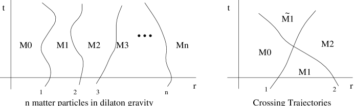
Figure 3: Particles Propagating in Dilaton Gravity

3.1 Trajectories That Do Not Intersect

In Appendix A we have implemented the procedure for eliminating the dilaton and the graviton described in the previous section. It turns out that the geometry between the particles looks like a slice of a black hole of fixed mass. This is illustrated in Figure 3 where $M_{i}/\lambda$ labels the mass outside the ith particle and $M_{0}/\lambda$ is the mass of the background black hole, if any. Furthermore, in a gauge with $R=\exp{\lambda r}$ and $L=1$ we obtain the following effective lagrangian for dressed massless particles:

$$L=\left(\frac{2}{\pi}\right)\sum_{i=1}^{N} \dot{r_{i}} \left\{e^{\lambda r_{i}}\left(\sqrt{M_{i-1}\pi}-\sqrt{M_{i}\pi}\right)\right.$$ (16)

$$\left.-\eta_{i}\lambda e^{2\lambda r_{i}}\ln\left(\frac{e^{\lambda r_{i}}-\eta_{i}\sqrt{M_{i}\pi}/\lambda}{e^{\lambda r_{i}}-\eta_{i}\sqrt{M_{i-1}\pi}/\lambda}\right)\right\}\>-\>\frac{M_{n}-M_{0}}{\lambda}$$

where $\eta_{i}$ is $+1$ for outgoing particles and $-1$ for infalling particles. This expression should be read as a Hamiltonian formulation of the Lagrangian ($L=\sum_{i}p_{i}\dot{r_{i}}-H$) so that $(M_{n}-M_{0})/\lambda$ is identified as the Hamiltonian of the system and the canonical momentum of the ith particle is:

$$p_{ci}=e^{\lambda r_{i}}\frac{2}{\pi}\left(\sqrt{M_{i-1}\pi}-\sqrt{M_{i}\pi}\right)-\eta_{i}\lambda e^{2\lambda r_{i}}\frac{2}{\pi}\ln\left(\frac{e^{\lambda r_{i}}-\eta_{i}\sqrt{M_{i}\pi}/\lambda}{e^{\lambda r_{i}}-\eta_{i}\sqrt{M_{i-1}\pi}/\lambda}\right)$$ (17)

This expression for the canonical momentum implicitly defines $M_{i}$ in terms of $M_{i-1}$ and $r_{i}$ and this chain of relations defines $M_{n}/\lambda$, the Hamiltonian, in terms of the coordinates and momenta of each of the particles. $M_{i}/\lambda$ should be thought of as the mass parameter of the geometry outside the ith particle and so $(M_{i}-M_{i-1})/\lambda$ can be understood as the energy of the ith particle.

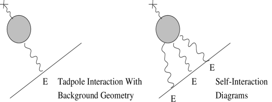
Figure 4: Diagrams Contributing to The Effective Lagrangian

3.2 Meaning Of The Effective Lagrangian

In order to understand the meaning of this effective Lagrangian it is useful to consider a single dressed particle whose Lagrangian is given by:

$$L=\left(\frac{2}{\pi}\right) \dot{r} \left\{e^{\lambda r}\left(\sqrt{M_{0}\pi}-\sqrt{M_{1}\pi}\right)\right.$$ (18)

$$\left.-\eta\lambda e^{2\lambda r}\ln\left(\frac{e^{\lambda r}-\eta\sqrt{M_{1}\pi}/\lambda}{e^{\lambda r}-\eta\sqrt{M_{0}\pi}/\lambda}\right)\right\}\>-\>\frac{M_{1}-M_{0}}{\lambda}$$

Here $M_{0}$ is the mass of the background black hole and $M_{1}$ is the ADM mass of the geometry. At large $r$ we can expand in powers of $\exp{-\lambda r}$ and we find that $p_{c}=\eta(M_{1}-M_{0})/\lambda+O(\exp{-\lambda r})$. This correctly tells us that near infinity, to leading order, the momentum of the massless particle equals its energy. We wish to interpret the effective Lagrangian in terms of the diagrams that have contributed to the dressing of the particle. In flat space we should have $p=E$, and in curved space the interaction with the background gives the classical equation $p=Ef(r)$ where $f(r)$ is a function of $r$ that can be read off from the geometry. In diagrammatic terms, the diagram proportional to $E$ in Figure 4 gives the classical description of a massless particle in curved space and the diagrams with more graviton legs represent the self-interaction corrections. Indeed, writing $E=(M_{1}-M_{0})/\lambda$ and linearizing Equation 18 we find that:

$$p=\eta E\frac{e^{\lambda r}}{e^{\lambda r}-\sqrt{M_{0}\pi}/\lambda}$$ (19)

This is exactly the relation between momentum and energy for a classical massless particle in the dilaton black hole in Equation 4. This agreement increases our confidence that we have correctly derived the effective theory and suggests that an expansion of $p_{c}$ in powers of $E=(M_{1}-M_{0})/\lambda$ amounts to a summation of the n-graviton self-interaction diagrams in Figure 4. The Lagrangian in Equation 16 contains graviton exchanges between all the particles in the system. We can truncate to exchanges of $k$ gravitons by expanding to the appropriate powers in the energies of each particle. Note that for outgoing particles ($\eta=+1$), Equation 18 tells us that a particle of finite energy has a momentum that blows up as $\exp{\lambda r}\rightarrow\sqrt{M_{1}\pi}/\lambda$. From the equations of motion computed below we will see that $\sqrt{M_{1}\pi}/\lambda$ is the location of the horizon and the blowup is symptomatic of the huge redshifts between the horizon and infinity.

3.3 Crossing Trajectories

Having understood the dressed Lagrangian describing particle trajectories that do not intersect we turn to the description of particles that cross each other. In the right hand Figure 3, we have two particles whose trajectories intersect. Before and after crossing the two particle Lagrangian 16 describes the system, but we must give a prescription for determining the the mass parameter $\tilde{M_{1}}$ that determines the geometry between the particles after crossing. ($M_{0}/\lambda$ and $M_{2}/\lambda$ are unchanged because the former is the mass of the background black hole and latter is the total conserved energy.) The splicing prescription is derived from the observation that the crossing of particles does not involve any actual displacement so that we expect total energy and momentum to be conserved. Applying this to the right hand Figure 3 and using the effective momenta given in Equation 17 we arrive at the splicing condition:

$$\left(e^{2\lambda r_{c}}-\frac{M_{0}\pi}{\lambda^{2}}\right)\left(e^{2\lambda r_{c}}-\frac{M_{2}\pi}{\lambda^{2}}\right)=\left(e^{2\lambda r_{c}}-\frac{M_{1}\pi}{\lambda^{2}}\right)\left(e^{2\lambda r_{c}}-\frac{\tilde{M}_{1}\pi}{\lambda^{2}}\right)$$ (20)

where $r_{c}$ is the position at which the crossing occurs. Letting $M_{b}/\lambda=(M_{2}-M_{1})/\lambda$ and $\tilde{M}_{b}/\lambda=(\tilde{M}_{1}-M_{0})/\lambda$ be the energies of the infalling particle before and after collision with the outgoer we can write the splicing condition as:

$$\frac{\tilde{M}_{b}\pi}{\lambda^{2}}=\frac{M_{b}\pi}{\lambda^{2}}+\frac{(M_{b}\pi/\lambda^{2})(M_{a}\pi/\lambda^{2})}{\left(e^{\lambda r_{c}}+\sqrt{M_{1}\pi}/\lambda\right)\left(e^{\lambda r_{c}}-\sqrt{M_{1}\pi}/\lambda\right)}$$ (21)

Here $M_{a}/\lambda$ is the energy of the outgoing particle prior to the collision. We see that the energy of the infaller is shifted by the collision. The significance of this shift will be discussed in Section 6.

3.4 Equations of Motion

To complete the description of the dressed classical mechanics of particles in dilaton gravity we must compute the equations of motion since the classical trajectories will be necessary for the WKB quantization of the theory in the next section. Since we are in the Hamiltonian formalism the equations of motion are given by $\dot{r}_{i}=\partial H/\partial p_{i}=(1/\lambda)\partial M_{n}/\partial p_{i}$ where all the $r_{i}$ and the $p_{j}$ for $j\neq i$ are held constant in taking the partial derivatives. Generically, the classical kinematics of a highly nonlinear Lagrangian like the one in Equation 16 can only be integrated if there are a sufficient number of conserved quantities present in the system. Fortunately, because neither the dilaton nor the graviton is dynamical we expect that the energy of every particle ($E_{i}=(M_{i}-M_{i-1})/\lambda$) is individually conserved in the absence of crossing of trajectories.

It is shown in Appendix B that the system of $n$ dressed particles is classically integrable since the $M_{i}$ are time-independent and have mutually vanishing Poisson brackets. With this observation in hand, we derive the equations of motion by noting from Equation 17 that the Hamiltonian $M_{n}/\lambda$ on depends on $p_{i}$ only via its dependence on $M_{n-1}$ which in turn depends on $M_{n-2}$ and so on until we reach $M_{i}$ which is implicitly expressed as a function of $p_{i}$. So we have $\dot{r}_{i}=(\partial M_{n}/\partial M_{n-1})_{r_{i},p_{i}}\cdots(\partial M_{i+1}/\partial M_{i})_{r_{i+1},p_{i+1}}(\partial M_{i}/\partial p_{i})_{r_{i},M_{i-1}}$. These derivatives can be computed by differentiating both sides of Equation 17 and rearranging terms. The subscripts indicate the variables in Equation 17 that are to be held constant while taking the derivatives. Putting everything together we find the equations of motion for the dressed particles:

$$\dot{r}_{i}=\left(\eta_{i}-\frac{\sqrt{M_{i}\pi}}{\lambda e^{\lambda r_{i}}}\right)\frac{e^{\lambda r_{n}}-\eta_{n}\sqrt{M_{n}\pi}/\lambda}{e^{\lambda r_{i+1}}-\eta_{i+1}\sqrt{M_{i}\pi}/\lambda}\prod_{k=i+1}^{n-1}\left(\frac{e^{\lambda r_{k}}-\eta_{k}\sqrt{M_{k}\pi}/\lambda}{e^{\lambda r_{k+1}}-\eta_{k+1}\sqrt{M_{k}\pi}/\lambda}\right)$$ (22)

The integrability of the system now comes to our rescue - all the $M_{i}$ are constant and so we can integrate the equation of motion of the outermost particle, use the trajectory to integrate the motion of the next inner particle and so on until all the classical trajectories have been computed. If particle trajectories cross we must use one set of $M_{i}$ prior to crossing and another after crossing following the splicing prescription described in the previous subsection. For use in the next section we integrate the equation of motion of a single dressed particle:

$$\dot{r}=\eta-\frac{\sqrt{M_{1}\pi}}{\lambda e^{\lambda r}}\>\>\>\>;\>\>\>\>(e^{\lambda r}-\eta\sqrt{M_{1}\pi}/\lambda)=e^{\eta\lambda t}(e^{\lambda r(0)}-\eta\sqrt{M_{1}\pi}/\lambda)$$ (23)

This equation of motion is identical to the equation for geodesic motion of a massless particle in the metric (4) for a black hole of mass $M_{1}/\lambda$. Indeed, for an outgoing trajectory ($\eta=+1$) we see that the particle can only escape to infinity if $e^{\lambda r(0)}>\sqrt{M_{1}\pi}/\lambda$. As discussed in Section 2 a black hole of mass $M_{1}/\lambda$ has its horizon at $e^{\lambda r}=\sqrt{M_{1}\pi}/\lambda$. We see that at the level of the equations of motion a single dressed particle moves as though the metric is determined by the total ADM mass ($M_{1}$) as opposed to just the mass of the background black hole ($M_{0}$).

We would like to use the effective Lagrangian in Equation 16 to construct the quantum mechanics of the system. Given $N$ particles we have a dressed Lagrangian that describes the propagation of these particles within $N$ particle Fock space. We need not be disturbed that the lack of a second quantized formulation will prevent us from seeing the particle production associated with the Hawking radiation. The Hawking flux is not associated with “vertices” in the usual perturbative sense of particle production - the Hawking particles appear because of a mismatch of vacua between the inertial pbserver at the horizon and the observer at inifinty. Given that we are in the N-particle Fock space we do not expect the number of particles to change via interactions between the $N$ particles. Therefore, given that $N$ Hawking particles are produced, we can study their back reaction effects by constructing the quantum mechanics described by the Lagrangian 16 within the $N$ particle Fock space. Nevertheless, there is a difficulty with quantizing the system of gravitationally dressed particles. Because the Lagrangian is so nonlinear in the coordinates and momenta we cannot simply promote these quantities to operators and canonically quantize the system since we would be faced with difficult normal ordering problems. The most reasonable procedure towards quantizing the system appears to be to study the semiclassical limit in which $\hbar\rightarrow 0$ so that action of classical trajectories of the particles and the small fluctuations around these trajectories dominate the quantum physics. In the next section we will describe the WKB procedure for carrying out such a quantization and then we will apply the procedure to computing the wavefunctions of the dressed particles. The resulting states presumably include all the self-interaction corrections arising from self-exchange of the longitudinal graviton and dilaton.

4 Computation of Dressed Wavefunctions

We are forced to resort to semiclassical methods to quantize the effective theory because it is too nonlinear for canonical or full path integral quantization. The basic idea of the semiclassical method is to observe that in the limit of small $\hbar$, the transport of wavefunctions is dominated by classical trajectories. (See Gutzwiller [21].) In general, if $\psi(r(0))=\rho(r(0))\exp{iS(r(0))}$ is the wavefunction at early times, the transport of the wavefunction to late times is described by the equation $\psi(r,t)=\int dr(0)\psi(r(0))K(r(0);r,t)$. Here $K$ is the propagator given by the path integral $K(r(0);r,t)=\int_{r(0)}^{r(t)}{\cal D}{\bf r}\exp{(i/\hbar)S({\bf r})}$ and $S$ is the action for the path ${\bf r}$. For small $\hbar$, extrema of the action dominate the path integral and the integral can be well approximated as the saddlepoint phase times the determinant of the quadratic fluctations around the saddlepoint. To use the semiclassical propagator to calculate the transport of wavefunctions we must calculate the above integral over the initial positions $r(0)$. Because the propagator has been calculated by the method of saddlepoints, it is only consistent to do the integral over $r(0)$ by the method of saddlepoints as well. It is useful to note that the phase of the integrand is proportional to $1/\hbar$ whereas the amplitude is $O(1)$ so that the saddlepoint is consistently calculated from the phases alone. In other words, we evaluate the integrand at the coordinate $r(0)^{\prime}$ at which the phase of the intgrand is minimized and then we calculate the determinant of quadratic fluctuations around this point. Because it is suppressed by a power of $\hbar$, the amplitude $\rho$ does not enter the calculation of the determinant and is simply evaluated at the saddlepoint. Putting all these facts together we arrive at the following expression for the semiclassical propagation of a wavefunction that starts at $t=0$ as $\psi_{0}(r(0))=\rho(r(0))e^{\frac{i}{\hbar}S_{0}(r(0))}$:

$$\psi(r,t) = \rho(r_{0})\sqrt{\frac{|-\partial^{2}R(r,r_{0},t)/\partial r\partial r_{0}|}{-\left(\partial^{2}S_{0}(r_{0})/\partial r_{0}^{2}+\partial^{2}R(r,r_{0},t)/\partial r_{0}^{2}\right)}}e^{\frac{i}{\hbar}(S_{0}(r_{0})+R(r,r_{0},t))}$$

$$R(r,r_{0},t) = \int_{r_{0}}^{r}p(r^{\prime},E)dr^{\prime}-Et$$ (24)

In this expression $E$ and $r_{0}$ are the self consistent solutions to the equations:

$$r=r(r_{0},E,t)\>\>\>;\>\>\>\frac{\partial S_{0}}{\partial r_{0}}=p(r_{0},E)$$ (25)

The first of these equations is the equation of motion for the classical trajectory of energy $E$ that starts at $r_{0}$ and the second equation is standard relation between the action and the momentum of a classical particle. The semiclassical method requires that the frequency of the wavefunction varies sufficiently slowly for us to define a local energy in every segment of the wave. The content of the above equations is that this local energy at $r_{0}$ is transported along the classical trajectory of that energy that starts at $r_{0}$ and is deposited at the final point of the trajectory after a time $t$. As a final check note that imposing the condition that $E$ is constant giving an energy eigenstate can be shown to yield the following wavefunction:

$$\psi(r,t)=\frac{1}{\sqrt{\dot{r}}}e^{\frac{i}{\hbar}\left[\int^{r}p(r,E)\,dr-Et\right]}$$ (26)

This is the familiar WKB expression for energy eigenstates in one dimensional quantum mechanics. We now apply this formalism to the gravitational self-interaction of particles in dilaton gravity. Note that in computing overlap integrals of semiclassical wavefunctions it is only consistent to use the method of saddlepoints since the WKB wavefunctions have themselves been computed in that manner.

4.1 Self-Interaction Corrections To Radiation

We will now compute the self-interaction corrections to wavefunctions of single particles propagating in dilaton gravity. Having computed the dressed spectrum we will repeat the calculation of the Hawking radiation in Section 2 with the improved modes. In fact we will only work with the phase of the wavefunction because, as discussed above, the saddlepoints in the overlap integrals that give the Bogliubov coefficients are insensitive to the amplitude which is suppressed by a power of $\hbar$. Equation 24 says that the phase of the single particle dressed WKB wavefunction is given by $S(r,t)=S_{0}(r_{0})+\int_{r_{0}}^{r}p_{c}dr-(M_{1}-M_{0})t/\lambda$ where we have identified the energy of the particle as the ADM mass ($M_{1}/\lambda$) minus the mass of the background black hole, and where $p_{c}$ is the coefficient of $\dot{r}$ in Equation 18. We are interested in the self-interaction of the outgoing wavefunctions that are responsible for producing the Hawking radiation. Integrating $p_{c}$ we find:

$$R=\int p_{c}\,dr= \frac{1}{\pi}\left[e^{\lambda r}\left(\frac{\sqrt{M_{0}\pi}}{\lambda}-\frac{\sqrt{M_{1}\pi}}{\lambda}\right)+\left(\frac{M_{1}\pi}{\lambda^{2}}-e^{2\lambda r}\right)\ln\left(e^{\lambda r}-\frac{\sqrt{M_{1}\pi}}{\lambda}\right)\right.-$$ (27)

$$\left.\left(\frac{M_{0}\pi}{\lambda^{2}}-e^{2\lambda r}\right)\ln\left(e^{\lambda r}-\frac{\sqrt{M_{0}\pi}}{\lambda}\right)\right]$$

According to Equation 25 we must also self consistently solve for $M_{1}$ and $r_{0}$ using the equation of motion (Equation 23 ) and the initial condition $S_{0}$. We will imagine that the self-interactions are turned off until $t=0$ and the wavefunction starts in an outgoing Kruskal eigenstate as in Equation 6. So we take $S_{0}=(2k/\pi)(e^{\lambda r}-\sqrt{M_{0}\pi}/\lambda)$. The self-consistency conditions in Equation 25 are solved in Appendix C to arrive at the leading order dressed WKB phase at late times:

$$S(r,t)=\frac{2}{\pi}\frac{\sqrt{M_{0}\pi}}{\lambda}\left(\exp\left(\frac{k\lambda}{\sqrt{M_{0}\pi}}\right)-1\right)e^{-\lambda t}\left(e^{\lambda r}-\frac{\sqrt{M_{0}\pi}}{\lambda}\right)$$ (28)

The late time wavefunction is $e^{iS}$ and therefore looks exactly like the Kruskal eigenstate in the initial condition with a redefined frequency. Note that $(\sqrt{M_{0}\pi}/\lambda)(\exp(k\lambda/\sqrt{M_{0}\pi})-1)$ is $k$ to leading order for small $k$ so that states of small Kruskal momentum are unaffected. However, as we shall shortly see, virtual states of very large Kruskal momentum are responsible for the production of the hawking radiation and so this frequency redefinition is important for them.

Having computed the one-particle dressed wavefunctions we are in a position to analyze the physical effects arising from gravitational self-interaction. Kraus and Wilczek have found that such self-interactions cause a energy dependent shift of the radiation temperature for Schwarschild and Reissner-Nordstrom black holes ([14], [10]) and it is interesting to understand whether such effects can occur in the context of the two dimensional black holes. We have computed the dressed analogues of the Kruskal eigenstates above, and if we also compute the dressed energy eigenstates we can find the Bogliubov transformations responsible for producing the Hawking radiation. From Equations 26 and 27 we know that the phase of a dressed energy eigenstate is $S_{\omega}(r,t)=R(r)-\omega t$ with $(M_{1}-M_{0})/\lambda\equiv\omega$. In computing the dressed Kruskal eigenstates we assumed that the particles had small energies and expanded to leading order in these energies. Under the same assumptions, $S_{\omega}$ becomes:

$$S_{\omega}(r,t)=\frac{\omega}{\lambda}\ln\left(e^{\lambda r}-\frac{\sqrt{M_{0}\pi}}{\lambda}\right)-\omega t-\frac{\omega}{2\lambda}$$ (29)

Writing the dressed energy eigenstate as $\phi_{\omega}=e^{iS_{\omega}}$ (we are ignoring amplitudes) we can compute the Bogliubov tranformations between the dressed states using the relations (9). To be consistent within the semiclassical framework, the integrals in Equation 9 should be regarded as overlap integrals between the two dressed bases and should be carried out by the method of saddlepoints. Define $\omega^{\prime}/\lambda=(2/\pi)(\sqrt{M_{0}\pi}/\lambda)[\exp(k\lambda/\sqrt{M_{0}\pi})-1]$ and $u_{f}=e^{-\lambda t}(e^{\lambda r}-\sqrt{M_{0}\pi}/\lambda)$ so that the dressed Kruskal states are $\psi=\exp(i(\omega^{\prime}/\lambda)u_{f})$. Then the saddlepoints for the $\alpha$ and $\beta$ integrals occur at:

$$\alpha^{*}:\>e^{-\lambda t}=\frac{\omega}{\omega^{\prime}(e^{\lambda r}-\frac{\sqrt{M_{0}\pi}}{\lambda})}\>\>\>;\>\>\>\beta^{*}:\>e^{-\lambda t}=-\frac{\omega}{\omega^{\prime}(e^{\lambda r}-\frac{\sqrt{M_{0}\pi}}{\lambda})}$$ (30)

We are interested in the radiation of moderate $\omega$ seen by the asymptotic observer and so we see that the saddlepoint for $\alpha$ occurs at very late times. The saddlepoint time for $\beta$ is off the real axis, but also has a large real part. Because of this it is consistent to use the late time form of the dressed wavefunctions as we are doing. Ignoring amplitudes of wavefunctions, the saddlepoint integral gives:

$$\alpha^{*}_{\omega\omega^{\prime}}=e^{i(3\omega/2\lambda)}\left(\frac{\omega^{\prime}}{\omega}\right)^{\frac{i\omega}{\lambda}}\>\>\>;\>\>\>\beta^{*}_{\omega\omega^{\prime}}=e^{i(3\omega/2\lambda)}\left(\frac{-\omega^{\prime}}{\omega}\right)^{\frac{i\omega}{\lambda}}=\alpha^{*}_{\omega\omega^{\prime}}e^{\frac{-\pi\omega}{\lambda}}$$ (31)

As in Section 2 $|\alpha_{\omega k}/\beta_{\omega k}|$ is independent of $k$ and so we reach the conclusion once again that the dressed energy eigenstates are thermally populated with a temperature of $(2\pi)/\lambda$ if the system is prepared in a state annihilated by the dressed Kruskal states.

We have not found a shift of the Hawking temperature unlike Kraus and Wilczek ([10, 11]). This is not surprising in retrospect because the temperature of dilaton black holes depends only on the cosmological constant and we do not expect the self-interactions of the matter particles to renormalize this quantity. Nonetheless, the frequency redefinition derived here is quite dramatic and we may wonder whether there are any physical effects associated with it. To resolve this question we would need to compute the amplitudes of the effective wavefunctions and examine whether the n-point functions of the Hawking state are changed. We do not expect any such changes because the frequency renormalization derived here does not mix positive and negative frequencies. The structure of the effective wavefunctions strongly suggests that the net effect of the self-interactions is merely a frequency redefinition.

In computing the Bogliubov tranformations we used only the leading order dressed wavefunctions in Equation 28. One may wonder whether the subleading corrections could lead to nonthermal population of states in the radiation. We do not expect this to happen because the computations in Appendix C show that the Kruskal eigenstates will depend on time via factors of $e^{-\lambda t}$. Consequently these states are periodic in imaginary time with a period of $2\pi/\lambda$ suggesting that the spectrum will look thermally populated even when the subleading terms are accounted for.

Before concluding this section there are two more useful lessons to draw. The first is that the Kruskal momenta contributing to late time radiation grow linearly with time and the second is that the self-interaction corrections are unimportant for infalling states. To show the first point we return to Equation 8 to express the dressed energy eigenstates in terms of the dressed Kruskal states: $\phi_{\omega}=\int d\omega^{\prime}(\alpha_{\omega\omega^{\prime}}\psi_{\omega^{\prime}}+\beta_{\omega\omega^{\prime}}\psi_{\omega^{\prime}}^{*})$. The $\omega\prime$ dependent part in integrand of the first term is $\exp(-i(\omega/\lambda){\ln{\omega^{\prime}}}+i(\omega^{\prime}/\lambda)u_{f})$ ($u_{f}$ is defined above). The saddlepoint that dominates the integral over $\omega\prime$ is at $\omega^{\prime}=\omega/u_{f}=\omega/(e^{-\lambda t}(e^{\lambda r}-\sqrt{M_{0}\pi}/\lambda))$ which grows exponentially in time at fixed $r$. Since $\omega^{\prime}\propto\exp(k\lambda/\sqrt{M_{0}\pi})$ for large $k$, we see that $k$ grows linearly in time.

Finally, we can ask whether incoming states are strongly affected by self-interactions. Physically, we do do not expect large effects because the relationship between momentum and energy for incoming particles does not become singular at horizon. The lack of any large effects can be shown in the WKB lanuguage by taking $S_{0}=(2k/\pi)(e^{\lambda r}+\sqrt{M_{0}\pi}/\lambda)$, so that we have an incoming Kruskal eigenstate as the initial condition, with $\eta=-1$ in Equation 17 for the canonical momentum. In the calculation of the dressed wavefunctions in Appendix C, the exponentiation of of the Kruskal frequency $k$ arises in the course of solving the WKB consistency conditions in Equation 25. It is a simple matter to show that the incoming initial conditions described above do not result in such an exponentiation for low energy incoming particles even in the region near the black hole horizon.

5 In-Out Scattering

Giddings and Nelson have carried out a calculation of the Hawking flux in the $1+1$ dilaton geometry produced by a classical infalling state ([19]). In this section we will study the radiation produced in the dynamical background of a quantum mechanical infalling state. A complete treatment of this problem involves consideration of the two-particle states in Fock space in which one particle is coming in and one particle is going out, treated with the two particle version of Lagrangian (16). The full problem is very hard to analyze because of the non-linearities of the gravitational interactions between the particles and because the self-interactions do not commute with the in-out scattering. We will consider the structure of the states in the full two particle Fock space in the next section and restrict ourselves to an approximate (and possibly more insightful) version of the problem here. First of all, we will semiclassically evolve an infalling quantum mechanical packet to produce a geometry whose ADM mass is uncertain and then we will study the Hawking problem in this background. By examining the form of the resulting scattering of the outgoing radiation we are able to identify the in-out scattering matrix for an arbitrary infalling state up to certain ordering problems. This will enable us to identify the effect an arbitrary infalling state has on the spectrum of outgoing particles. From this identification we are able to draw some qualitative conclusions regarding the return of information in the radiation in the presence of the full self-interactions.

We now want to construct two-particle WKB wavefunctions. This can be done in the same way as discussed at the beginning of Section 4. The phase of the two particle wavefunction is given by $S(r_{a},r_{b},t_{a},t_{b})=S_{0}(r_{a}(0),r_{b}(0))+\int p_{a}dr_{a}+\int p_{b}dr_{b}-E_{a}t_{a}-E_{b}t_{b}$. In this equation we have two times $t_{a}$ and $t_{b}$ because we may choose to evolve the incoming part of the two particle wavefunction forward for a different amount of time from the outgoing part of the wavefunction. As in the one particle case we must solve self-consistently for $E_{a},E_{b},r_{a}(0)$ and $r_{b}(0)$ in terms of $r_{a},r_{b},t_{a}$ and $t_{b}$ by using the two equations of motion and the initial conditions that $\partial S_{0}(r_{a}(0),r_{b}(0))/\partial r_{a}(0)=p_{a}(r_{a}(0))$ and $\partial S_{0}(r_{a}(0),r_{b}(0))/\partial r_{b}(0)=p_{b}(r_{b}(0))$. In this section we are interested in the effect an incoming state has on the outgoing radiation. So we will take $t_{b}=0$ so that the incoming state is not evolved forward in time at all - we simply specify the incoming state at $t=0$ and compute its effects on the outgoing part of the wavefunction. In other words, instead of specifying the two particle configuration space as $\{r_{a},r_{b}\}$ at some time $t$ we choose the configuration space to be $\{r_{a},r_{b}(0)\}$ and write the wavefunction in terms of these coordinates. Furthermore we will prepare the system at $t=0$ so that $S_{0}(r_{a}(0),r_{b}(0))=S_{0a}(r_{a}(0))+S_{0b}(r_{b}(0))$ - in other words, the incoming and outgoing wavefunctions are not entangled at $t=0$ either by assuming that the interactions are turned off at earlier times or by picking well separated initial wavepackets. As in Section 4 wavefunction amplitudes in the semiclassical approximation are computed as determinants of fluctuations around saddlepoints and are relatively unimportant since they are suppressed by a power of $\hbar$. For this reason we will omit them as we did in the previous section.

5.1 Leading Order In-Out Scattering

We begin by turning off the self-interactions in order to understand the effects of the in-out interactions by themselves. The effects of self-interactions are considered in Section 5.4.

Consider an incoming quantum wavepacket propagating in the background of a black hole of mass $M_{0}/\lambda$. The state is specified by an initial wavefunction $\psi_{b0}=\rho_{0}\exp{iS_{b0}(r_{b}(0))}$. Removing the self-interactions amounts to keeping only the tadpole diagram proportional to $E$ in Figure 4 and so we will call this the “tadpole approximation”. As discussed in Section 3.1 this can be achieved by linearizing the relation between the momentum and energy of a particle in Equation 17. Doing this gives the following relations:

$$p_{b}=-\frac{M_{b}}{\lambda}\frac{e^{\lambda r_{b}}}{e^{\lambda r_{b}}+\frac{M_{0}\pi}{\lambda}}\>\>;\>\>\dot{r}_{b}=-1-\frac{\sqrt{M_{0}\pi}}{e^{\lambda r_{b}}\lambda}$$ (32)

Integrating this equation of motion we find that the classical trajectories dominating the evolution of the infalling wavepacket have the equations:

$$\left(e^{\lambda r_{b}}+\frac{\sqrt{M_{0}\pi}}{\lambda}\right)=e^{-\lambda t}\left(e^{\lambda r_{b}(0)}+\frac{\sqrt{M_{0}\pi}}{\lambda}\right)$$ (33)

If the the initial wavepacket is not an energy eigenstate, then the geometry will not be in an eigenstate of the ADM mass. Indeed, identifying $p_{b0}=\partial S_{b0}/\partial r_{b}(0)$ as the momentum of the initial state, the relations in Equation 32 tell us that the sector of the wavefunction dominated by the classical trajectory starting at $r_{b}(0)$ has an ADM mass given by:

$$\frac{M_{2}}{\lambda}\equiv\frac{M_{0}+M_{b}}{\lambda}=\frac{M_{0}}{\lambda}+e^{-\lambda r_{b}(0)}\left(e^{\lambda r_{b}(0)}+\frac{\sqrt{M_{0}\pi}}{\lambda}\right)\left(-\frac{\partial S_{b0}}{\partial r_{b}(0)}\right)$$ (34)

We can use these observations to carry out the semiclassical evolution of outgoing states in the quantum background produced by the state $\psi_{b0}$.

Consider an outgoing wavefunction propagating in the background produced by the infalling packet. Prior to crossing the infalling state the outgoer travels in a background of mass $M_{0}/\lambda$ and after crossing the background has a mass $M_{2}/\lambda$ which depends on the sector of the infalling state under consideration. Removing the self-interactions of the outgoer by linearizing Equation 17 gives:

$$before:p_{a}=\frac{M_{a}}{\lambda}\frac{e^{\lambda r_{a}}}{e^{\lambda r_{a}}-\frac{\sqrt{M_{0}\pi}}{\lambda}}\>\>\>;\>\>\>after:p_{a}=\frac{\tilde{M}_{a}}{\lambda}\frac{e^{\lambda r_{a}}}{e^{\lambda r_{a}}-\frac{\sqrt{M_{2}\pi}}{\lambda}}$$ (35)

where $M_{a}/\lambda$ is the energy of the trajectory before the collision and $\tilde{M}_{a}/\lambda$ is the energy after the collision. The equations of motion before and after crossing are:

$$before: \>\dot{r}_{a}=\left(1-\frac{\sqrt{M_{0}\pi}}{e^{\lambda r_{a}}\lambda}\right)\>\>;\>\>e^{\lambda r_{a}}-\frac{\sqrt{M_{0}\pi}}{\lambda}=e^{\lambda t}\left(e^{\lambda r_{a}(0)}-\frac{\sqrt{M_{0}\pi}}{\lambda}\right)$$ (36)

$$after: \>\dot{r}_{a}=1-\frac{\sqrt{M_{2}\pi}}{e^{\lambda r_{a}}\lambda}\>\>\>;\>\>\>\left(e^{\lambda r_{a}}-\frac{\sqrt{M_{2}\pi}}{\lambda}\right)=e^{-\lambda(t-t_{c})}\left(e^{\lambda r_{c}}-\frac{\sqrt{M_{2}\pi}}{\lambda}\right)$$ (37)

where $t_{c}$ and $r_{c}$ are the time and position at which the outgoing classical trajectory intersects with the incoming classical trajectory that starts at $r_{b}(0)$. This completes the specification of the leading order classical mechanics of the outgoing particles in the backgrounds produced by the infalling quantum state. These ingredients will be used in the next section to compute the approximate semiclassical quantum mechanics of the outgoing states in the quantum infalling background.

5.2 Tadpole Corrected Two-Particle Wavefunctions

As discussed earlier the phase of the two particle wavefunction is given by:

$$S(r_{a},t,r_{b}(0))=S_{b0}(r_{b}(0)) + S_{a0}(r_{a}(0))+\int_{r_{a}(0)}^{r_{c}}p_{a}dr_{a}$$ (38)

$$+ \int^{r_{a}}_{r_{c}}p_{a}dr_{a}-M_{a}t_{c}/\lambda-\tilde{M}_{a}(t-t_{c})/\lambda$$

(We have split the usual integral $\int(p\,dr-H\,dt)$ into the parts before and after crossing.) Performing the integrals we find:

$$\int p_{a}dr_{a}=\frac{\tilde{M}_{a}}{\lambda^{2}}\ln\left[\frac{e^{\lambda r_{a}}-\sqrt{M_{2}\pi}/\lambda}{e^{\lambda r_{c}}-\sqrt{M_{2}\pi}/\lambda}\right]+\frac{M_{a}}{\lambda^{2}}\ln\left[\frac{e^{\lambda r_{c}}-\sqrt{M_{0}\pi}/\lambda}{e^{\lambda r_{a}(0)}-\sqrt{M_{0}\pi}/\lambda}\right]$$ (39)

Note that the equations of motion 36 and  37 tell us the ratios within the logarithms in terms of the time travelled before and after the collision with the infaller. Using these relations in Equation 39 we find that the phase of the two particle wavefunction in the tadpole approximation is given by:

$$S(r_{a},t,r_{b}(0))=S_{b0}(r_{b}(0))+S_{a0}(r_{a}(0))$$ (40)

So we need only solve for $r_{a}(0)$ as a function of $r_{a}$, $t$ and $r_{b}(0)$ in order to compute the WKB phase of the two-particle wavefunction.

Let us take $S_{a0}=(k/\lambda)(e^{\lambda r_{a}(0)}-\sqrt{M_{0}\pi}/\lambda)$ so that we have an outgoing Kruskal eigenstate. Using the equations of motion of the outgoing particle before and after scattering it is easy to write $r_{a}(0)$ in terms of $r_{a}$, $t$ and $r_{c}$ where $r_{c}$ is the position at which the collision with the infaller occurs. Next we use the equations of motion of the infaller before scattering along with the equation of motion of the outgoer after scattering to find that:

$$\left(e^{\lambda r_{c}}+\frac{\sqrt{M_{0}\pi}}{\lambda}\right)\left(e^{\lambda r_{c}}-\frac{\sqrt{M_{2}\pi}}{\lambda}\right)=u_{out}v_{in}$$ (41)

where we have defined $u_{out}=e^{-\lambda t}(e^{\lambda r_{a}}-\sqrt{M_{2}\pi}/\lambda)$ and $v_{in}=(e^{\lambda r_{b}(0)}+\sqrt{M_{0}\pi}/\lambda)$. At late times on ${\cal I}^{+}$, which is the region of interest to us, the solution to the equation is:

$$e^{\lambda r_{c}}\approx\frac{\sqrt{M_{2}\pi}}{\lambda}+\frac{u_{out}v_{in}}{\sqrt{M_{2}\pi}/\lambda+\sqrt{M_{0}\pi}/\lambda}$$ (42)

Using this late time solution for $\exp{\lambda r_{c}}$ in the outgoing equations of motion yields a solution for $\exp{\lambda r_{a}(0)}$ that gives the following result for the phase of the outgoing part of the wavefunction:

$$S(r_{a}(0))=\frac{k}{\lambda}e^{-\lambda t}\left(e^{\lambda r_{a}}-\frac{\sqrt{M_{2}\pi}}{\lambda}\right)+\frac{\pi}{\lambda^{2}}\left(k\frac{(M_{2}-M_{0})/\lambda}{v_{in}}\right)$$ (43)

Finally, we can use Equation 34 for the mass of the geometry $M_{2}/\lambda$ in the sector of the two-particle wavefunction labelled by $r_{b}(0)$. The semiclassical method is only valid when the energy of the incoming state is small compared to the mass of the black hole ($M_{b}\ll M_{0}$) so that we can expand the $\sqrt{M_{2}\pi}$ to leading order arriving at the following expression for the phase of the two-particle WKB wavefunction:

$$S(r_{a},t,r_{b}(0))= S_{b0}(r_{b}(0))+\frac{P_{-}}{\lambda}e^{-\lambda t}\left(e^{\lambda r_{a}}-\frac{\sqrt{M_{0}\pi}}{\lambda}\right)+$$ (44)

$$\frac{\pi}{\lambda^{2}}P_{-}\left[1-\frac{\lambda e^{-\lambda t}v_{in}}{2\sqrt{M_{0}\pi}}\right]P_{+}$$

where we have identified $P_{-}\equiv k$ as the outgoing Kruskal momentum and $P_{+}=M_{b}/v_{in}=\exp{-\lambda r_{b}(0)}(-\partial S_{b0}/\partial r_{b}(0))$ as the Kruskal momentum flowing in from the initial coordinate $r_{b}(0)$. Comparing with Equation 6 for the outgoing Kruskal eigenstates we see that the last expression has the structure of a scattering phase shift induced in the outgoing state by the incoming state.

5.3 Tadpole Corrected Physics

First let us examine the structure of the two particle wavefunction in Equation 44. The leading term on the second line, $\pi P_{-}P_{+}/\lambda^{2}$ is the two dimensional reduction of the shockwave interaction first advocated by t’Hooft ([3],[5, 6]). The term that is suppressed by $\sqrt{M_{0}\pi}$ arises because the position of the horizon moves when the infalling state falls into the black hole. This shift of the horizon “squeezes” the region outside the black hole causing a deformation of the wavefunction of states defined in the exterior region. In general, the term on the second line represents a scattering phase shift produced in the outgoing state by the incoming state and has a structure somewhat reminiscent of the exact S-matrix in the electromagnetic analogue problem studied by [22]. However, we do not expect the subleading correction computed here to restore the information about the infalling state to infinity since we do not have a systematic series of such corrections of the necessary structure.

The two particle wavefunction in Equation 44 can be used to identify the scattering operator that acts on the outgoing state in the presence of the infalling wavepacket. To do this observe that in the WKB method operators are essentially replaced by expectation values taken locally in every segment of the wavefunction with slowly varying phase. For example, the quantity $P_{+}=\exp{-\lambda r_{b}(0)}(-\partial S_{b0}/\partial r_{b}(0))$ is to be understood as an expectation value of $P_{+}$ taken locally in the neighbourhood of $r_{b}(0)$. Indeed, identifying the momentum $p_{b}(0)=\partial S_{b0}/\partial r_{b}(0)$ (and similarly $p_{a}$) we can promote the coordinates and momenta appearing in the scattering phase shift computed above to operators and arrive at the scattering operator acting on the outgoing states up to ordering problems. This scattering operator has the effect of entangling the outgoing and incoming states.

Next, we calculate the Hawking radiation in the dynamical background produced by the incoming state via computation of the Bogliubov coefficients. In order to do this we need the the form of the energy eigenstates as measured by the asymptotic observer. Using Equation 26 we find the phase of an asymptotic energy eigenstate to be:

$$S_{\omega}(r_{a},t,r_{b}(0)) = S_{b0}(r_{b}(0))+\int^{r}p_{a}dr_{a}-\omega t$$ (45)

$$= S_{b0}(r_{b}(0))+\frac{\omega}{\lambda}\ln\left(e^{\lambda r_{a}}-\frac{\sqrt{M_{2}\pi}}{\lambda}\right)-\omega t$$

Note that $S_{\omega}$ diverges at $\exp{\lambda r_{a}}=\sqrt{M_{2}\pi}/\lambda$ where the horizon of the black hole is located after the infalling mode has fallen in. In previous sections we have only worked with states defined in the exterior of the black hole but in what follows we will need to augment the wavefunctions $\exp{iS_{\omega}}$ with modes defined in the interior of the black hole. This is necessary because the Kruskal eigenstates in our initial conditions have support both inside and outside the black hole and therefore a full analysis of the final state requires modes defined in both these regions. Since the definition of a “particle” is somewhat ambiguous inside the black hole, we are free to pick any convenient basis to augment the set $\phi_{\omega}=\exp{iS_{\omega}}$. In the interior of the black hole we therefore pick the set $\hat{\phi}_{\omega}=\exp{i\hat{S}_{\omega}}$ where:

$$\hat{S}_{\omega}(r_{a},t,r_{b}(0))=S_{b0}(r_{b}(0))+\frac{\omega}{\lambda}\ln\left(\frac{\sqrt{M_{2}\pi}}{\lambda}-e^{\lambda r_{a}}\right)-\omega t$$ (46)

In Equation 8 we had defined the Bogliubov coefficients $\alpha$ and $\beta$ relating $\phi_{\omega}$ to the Kruskal basis. Now define $\hat{\alpha}$ and $\hat{\beta}$ analogously to relate $\tilde{\phi}_{\omega}$ to the Kruskal states. Using the relations 9 and their analogues for $\hat{\alpha}$ and $\hat{\beta}$ we find that saddlepoint calculations give the following results:

$$\alpha^{*}_{\omega k}(r_{b}(0)) = e^{i\pi kP_{+}/\lambda^{2}}e^{i\omega/\lambda}\left(\frac{k}{\omega}\right)^{i\omega/\lambda}$$

$$\beta^{*}_{\omega k}(r_{b}(0)) = -e^{-i\pi kP_{+}/\lambda^{2}}e^{i\omega/\lambda}\left(\frac{-k}{\omega}\right)^{i\omega/\lambda}=-\alpha^{*}_{\omega k}\,e^{-\pi\omega/\lambda}$$

$$\hat{\alpha}^{*}_{\omega k}(r_{b}(0)) = \alpha^{*}_{\omega k}(r_{b}(0))\;e^{\pi\omega/\lambda}\>\>\>\>\>;\>\>\>\>\>\hat{\beta}^{*}_{\omega k}(r_{b}(0))=\beta^{*}_{\omega k}(r_{b}(0))\;e^{\pi\omega/\lambda}$$ (47)

We have written these Bogliubov coefficients as functions of $r_{b}(0)$ in order to emphasize that $P_{+}=\exp{-\lambda r_{b}(0)}(-\partial S_{b0}/\partial r_{b}(0))$ is a function of $r_{b}(0)$ and that the in-out scattering represents an entanglement that prevents us from separating the Hilbert space into a product of incoming and outgoing states.

Despite the entanglement produced by the scattering, since $|\alpha_{\omega k}/\beta_{\omega k}|$ is independent of both $k$ and $r_{b}(0)$, the standard arguments used in Section 2 tell us that the Kruskal vacuum state contains a thermal spectrum of particles of temperature $2\pi/\lambda$. (See [19] and [20] for explanations of the standard arguments.) Indeed, we can show that the final Hawking state is left completely unaffected by the $P_{+}P_{-}$ phase accumulated during the in-out scattering. To show this, let $a_{k}$ be the annihilation operator for the Kruskal mode $k$ and let $b_{\omega}$ and $\hat{b}_{\omega}$ be the annihilation operators for the asymptotic modes $\phi_{\omega}$ and $\hat{\phi}_{\omega}$ defined in the previous section. Then the Bogliubov coefficients can be used to relate the various creation and annihilation operators ([19]):

$$a_{k}=\int dw\,\left[\alpha_{\omega k}\,b_{\omega}+\beta^{*}_{\omega k}\,b^{+}_{\omega}+\hat{\alpha}_{\omega k}\,\hat{b}_{\omega}+\hat{\beta}^{*}_{\omega k}\,\hat{b}^{+}_{\omega}\right]$$ (48)

The state of the system is defined to be the one that is annihilated by all the operators $a_{k}$. Putting in the Bogliubov coefficients in Equation 47 it is clear that the scattering phase can be factored out of Equation 48 giving:

$$a_{k}=e^{-i\pi kP_{+}/\lambda^{2}}a_{k}^{\prime}$$ (49)

where $a_{k}^{\prime}$ is the Kruskal annihilation operator in the absence of the scattering phase shifts. Since the Hawking state in the absence of scattering is the one annihilated by all the $a_{k}^{\prime}$ we can see that the same state is annihilated by the $a_{k}$ so that the in-out scattering does not affect the state at all. Indeed, the only trace of the infalling state in the radiation is that the energy eigenstates are defined in a geometry whose mass is determined by the energy carried into the black hole by the infaller.

5.4 In-Out Scattering With Self-Interaction

In previous sections we have computed the effects on the Hawking radiation of self-interactions and of an infalling state. The former led to a renormalization of the frequency of outgoing Kruskal states and the latter produced a scattering phase shift. We may wonder whether the two effects together can be responsible for any added recovery of information. The problem is that the severe non-linearities of the self-interacting system in the presence of an incoming state preclude analysis except in very special kinematical regimes. Therefore, despite extensive calculations in the more complete scenario we will be satisfied with a qualitative discussion of the phenomena that can be expected.

The in-out scattering does not commute with the self-interactions since the scattering shifts the phase of the wavefunction by an amount proportional to the outgoing Kruskal momentum and the self-interactions renormalize this momentum. Let us imagine that the self-interactions are turned off until $t=0$. Then as time passes, the wavefunction gradually renormalizes its Kruskal momentum $k$ to $[\exp\left(k\lambda/\sqrt{M_{0}\pi}\right)-1]$. The scattering phase shift acquired upon interaction with the incoming state will depend on how far the state has been permitted to renormalize itself. This can potentially leave a trace of the time of interaction in the outgoing wavefunction thereby carrying out some information regarding the composition of the incoming wavepacket. Careful scrutiny shows that the particular feature of the self-interacted wavefunctions that could carry this information would be the shifts $\epsilon$ and $\delta$ in exponent on the right side of Equation 74. These quantities are expected to be shifted by the interaction with the infaller and will not cancel in the final state like the $P_{+}P_{-}$ shifts in the previous section. In other words, the in-out interactions could affect the renormalization of the Kruskal frequency in such a way as to enable some return of information.

6 Are Semiclassical Methods Valid?

The results of previous sections appear to demonstrate that self-interactions and the in-out scattering have little effect on the late time radiation despite dramatic effects on the individual states involved in the computation. In this section we will address some consequences of the fact that the results in the previous sections also demonstrate that the semiclassical approximation is breaking down rapidly.

To see this, note that the semiclassical methods are only valid when the energies of the particles involved are small. Now, given the Bogliubov coefficients in Equation 47, an energy eigenstate of energy $\omega$ in the region outside the black hole can be constructed from the Kruskal states as $\phi_{\omega}=\int dk\,\left[\alpha_{\omega k}\psi_{k}+\beta_{\omega k}\psi_{k}^{*}\right]$. It is easily shown that this integral is dominated by modes with:

$$k\sim\frac{\omega}{e^{-\lambda t}\left(e^{\lambda r_{a}}-\sqrt{M_{2}\pi}/\lambda\right)}$$ (50)

Since the typical late time radiation has energy $\lambda/2\pi$, this means that the modes that contribute to the Hawking flux have a Kruskal momentum $k$ that is growing exponentially in time.

Now, the equation $\partial S_{a0}/\partial r_{a}(0)=p_{a}(r_{a}(0))$ combined with Equation 35 before the collision and the Kruskal initial condition for $S_{a0}$ gives the relation $\frac{M_{a}}{\lambda}=k(e^{\lambda r_{a}(0)}-\sqrt{M_{0}\pi}\lambda)$. Using the solution for $\exp{\lambda r_{a}(0)}$ arrived at in Section 5.2 we find that the energy of the outgoing state prior to scattering from the incoming state is given by:

$$\frac{M_{a}}{\lambda}=ke^{-\lambda t}\left(e^{\lambda r_{a}}-\frac{\sqrt{M_{2}\pi}}{\lambda}\right)+\frac{\pi kP_{+}}{\lambda^{2}}$$ (51)

with $P_{+}=\exp{-\lambda r_{b}(0)}(-\partial S_{b0}/\partial r_{b}(0))$. Since $k$ is growing exponentially in time we see that the Hawking flux emerges from states dominated by classical trajectories that have exponentially high energies before collision with the infalling state. At the formal level this invalidates the semiclassical approach and suggests that the results of previous sections should not be believed.

Figure 5: Diagrams Contributing to The Hawking State

In the calculation of the Hawking radiation, there are no real particles in the system that have these high energies since the state is defined to be the Kruskal vacuum. Therefore, a common argument says, the large shifts described above do not threaten the validity of the semiclassical computations. However, the calculation of the misalignment of Kruskal and asymptotic vacua requires use of the Bogliubov coefficients which depend on the excited states of the system. So, even if the system is placed in an initial state which apparently acquires no semiclassical corrections (being a state of Kruskal momentum zero) the calculation of Bogliubov coefficients has limited validity because of the large corrections to the excited states. Put another way, the precise form of the vacuum redefinition depends on the behaviour of modes of nonzero Kruskal momentum which acquire large corrections. A way to see this explicitly is in the formula for the Hawking state $\exp(b^{+}\beta^{*}\alpha^{-1}b^{+})|0>$ where $\alpha$ and $\beta$ are “matrices” of Bogliubov coefficients $\alpha_{\omega k}$ and $\beta_{\omega k}$ and the operators $b_{\omega}^{+}$ create asymptotic states. (This can be derived as the solution to the condition that the Hawking state is annihilated by the Kruskal mode operators ( [19, 20]).) This formula has the structure of pairs of particles coming out of some loop diagram as in Figure 5. The matrix product $\beta^{*}\alpha^{-1}$ involves a sum on intermediate Kruskal states and is essentially a summation over the particles running around the loops in Figure 5. As discussed earlier, the states in these loops have energies that grow exponentially with time prior to scattering from the incoming state. This suggests that we simply do not have sufficient control over the summation on virtual processes implicit in the computation of the Hawking state to be able to believe that the semiclassical results have exact validity.

We may fear that the results presented here are gauge dependent since we are working with a particular parametrization of the dilaton black hole. However, this fear is allayed by observing that the method of this paper is to compute the the WKB phase which is given by $\int p\,dr$, a reparametrization invariant quantity. So the exponentially large scattering phase shifts that threaten the validity of the semiclassical calculations should appear in any parametrization including one that only uses the “nice slices” of [23]. Another objection that is sometimes raised is that arguments regarding the breakdown of the semiclassical approximation involve “postdiction” whereby we try to reason about the states from which a low energy state at the current time could have developed. It has been argued that difficulties with such “postdiction” should not be interpreted as evidence for breakdown of the semiclassical theory ([23]). In fact, the problem should rather be phrased in terms of the structure of the Hilbert space on which the field theory is defined as we will discuss in the next section.

6.1 Structure of The Hilbert Space and Complementarity

As discussed above, the Hawking state is calculated by computing the misalignment between the vacuum defined by inertial observers at the black hole horizon and by obervers at infinity. This misalignment depends on the structure of the excited states of the system. In the presence of infalling matter, the Hilbert space contains both an infalling and outgoing component. In Section 5.1 the states in this in-out Hilbert space were approximated by removing the self-interactions and by having the infalling state propagate in the static background black hole while the outgoing state propagated in the quantum mechanical geometry thus produced. In fact, a complete treatment involves a study of two particle states with one infaller and one outgoer treated with the two particle version of the self-interacted Lagrangian 16. In this section we consider such two particle states and find that the interactions between the infaller and outgoer lead to serious difficulties with the definition of the Hilbert space.

Using the conventions of the right-hand Figure 3 we take $M_{a}/\lambda=(M_{1}-M_{0})/\lambda$ and $M_{b}/\lambda=(M_{2}-M_{1})/\lambda$ to be the energies of the outgoing and incoming particles before scattering. Similarly, take $\tilde{M}_{a}/\lambda=(M_{2}-\tilde{M}_{1})/\lambda$ and $\tilde{M}_{b}/\lambda=(\tilde{M}_{1}-M_{0})/\lambda$ to be the energies of the outgoing and incoming particles after scattering. We will begin by assuming that all these energies are much smaller than the black hole mass so that the semiclassical treatment is valid and show that in the kinematical regime relevant to the Hawking radiation, we are driven well out of the regime of validity. The splicing prescription in Equation 21 gives $\tilde{M}_{b}$ in terms of the incoming energies and the position $r_{c}$ at which the scattering occurs. Using the splicing prescription and energy conservation with the two particle equations of motion derived in Section 3.4, we can imitate the analysis of the self-interactions and the in-out scattering in Sections 4.1 and 5.1. Define $u_{out}=(\exp{\lambda r_{a}}-\sqrt{M_{2}\pi}/\lambda)\exp{-\lambda t}$ and $v_{in}=(\exp{\lambda r_{b}(0)}+\sqrt{M_{2}\pi}/\lambda)$. Then, given some infalling energy $M_{b}/\lambda$, it is easy to show that at late times on $\cal{I}^{+}$, when $u_{out}\,v_{in}\ll M_{b}/\lambda^{2}\ll M_{0}/\lambda^{2}$, the following results hold in the leading order:

$$\frac{M_{a}}{\lambda} =\omega^{\prime}u_{out}+\frac{\pi}{\lambda^{2}}\frac{\omega^{\prime}\,M_{b}}{v_{in}}$$ (52)

$$\frac{\tilde{M}_{a}}{\lambda} =\omega^{\prime}u_{out}\>\>\>\>\>\>\>;\>\>\>\>\>\>\> \frac{\tilde{M}_{b}}{\lambda}=\frac{M_{b}}{\lambda}+\frac{\pi}{\lambda^{2}}\frac{\omega^{\prime}\,M_{b}}{v_{in}}$$ (53)

where we have defined the self-interaction renormalized frequency:

$$\omega^{\prime}=\frac{2}{\pi}\sqrt{M_{0}\pi}\left(e^{\left(k\lambda/\sqrt{M_{0}\pi}\right)}-1\right)$$ (54)

Here we have used the fact that the energies of the particles are assumed to be small to use the approximations made in the section on self-interaction corrections, as well as to drop some terms of order $O(M_{b}/M_{0})$ which give negligible corrections to the equations of motion of the outgoing particle prior to scattering.

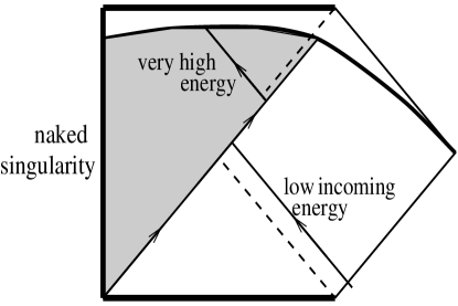
Figure 6: The black hole geometry corresponding to the two-particle scattering process between a low energy incoming mode and a typical outgoing mode. The interior geometry lies in the future of an unacceptable naked singularity and therefore its classical interpretation is suspect.

We are now in a position to extract the most important physical consequences of the self-interacted in-out scattering. First of all, the results on the self-interactions and in-out scattering have told us that the typical energy of the outgoing particle is unchanged from the classic result and will be $\tilde{M}_{a}/\lambda\sim\lambda/2\pi$. So, from Equation 53, $\omega^{\prime}\sim(\lambda/2\pi)/u_{out}$. From the definition of $u_{out}$ we see that $\omega^{\prime}$ is growing exponentially with time. Now consider a low energy mode dropped into the black hole with some small $M_{b}$. Looking at the solution for $M_{a}$, and using the exponential growth of $\omega^{\prime}$, we see that the state in the two particle Hilbert space responsible for producing the late-time Hawking radiation is dominated by classical trajectories with exponentially large energies before scattering from the infalling state.

The first lesson of these huge energy shifts is that states of absurdly high energies will have to be admitted into the Hilbert space on the early slice to produce the states on the late slice necessary to support the Hawking radiation. Furthermore, if we require that we are able to observe late time Hawking radiation of reasonable energies, then Equation 53 shows that low-energy infalling modes will necessarily be scattered by the outgoer into states inside the black hole with extremely large energies.

The huge energies developed by the particles can also be rewritten as the difference in the masses of the geometries on either side of the particle. If we would require the mass of the internal black hole $M_{0}/\lambda$ to remain fixed, the huge energies into which the infalling particle is scattered imply that we would have to admit states of absurdly high ADM mass into the late slice Hilbert space. This would clearly be unphysical. Instead, we should require that the total energy of the system, as given by the ADM mass, remains at some reasonable fixed values $M_{2}/\lambda$, and consider the states of the system with this total energy. In that case, the huge energies into which the infalling particles are scattered imply that the interior black hole geometry must have a negative mass thereby displaying a naked singularity. (See Figure 6.) Both alternatives, absurdly high energy states in the Hilbert space and naked singularity geometries, seem quite unpalatable.

There are two complementary ways to avoid both difficulties. The first is to require that the radiation observed at late times has exponentially small energies so that the states in the Hilbert space that are responsible for producing the radiation never have energies exceeding some finite cutoff. This allows the infalling matter to propagate into the black hole interior without developing very high energies on the late time slice. This prescription therefore gives a construction of a Hilbert space appropriate to an infalling observer. However, this seems like an unacceptable solution to an outside observer since it involves a drastic cutoff on the outgoing modes that tends to zero energy at late times. The complementary solution is to restrict the infalling modes to have exponentially small energies. Under this circumstance also, the states in the late time Hilbert space remain well defined. However, this prescription clearly imposes severe restrictions on the physics that the infalling observer can observe.

The dilemma seems to force the conclusion that the semiclassical theory of Hawking radiation, even with the self-interaction corrections, breaks down rapidly. Furthermore, there are two complementary, semiclassically controlled Hilbert spaces at late times. One is appropriate for describing the physics seen by the infaller, and the other is appropriate to a description of the Hawking radiation. It is possible that these complementary Hilbert spaces should be identified in some way giving a realization of black hole complementarity.

7 Conclusion

In this paper we have studied back-reaction effects in Hawking radiation from $1+1$ dilaton black holes. First of all, we constructed the effective theory produced by integrating out gravity and the dilaton and used this to study the self-interaction of the Hawking radiation. We found an unusual renormalization of the Kruskal frequency of outgoing states that nevertheless left the Hawking temperature unchanged. Then we studied the radiation issuing from a dynamical background produced by a quantum mechanical state falling into a black hole. This calculation was carried out in an approximation where the self-interactions were removed in order to examine the scattering effects separately. The in-out interaction was found to produce large scattering phases in outgoing states that nevertheless conspire to leave the Hawking state essentially unchanged. Finally, we asked whether these semiclassical conclusions could be trusted. We displayed the evidence that semiclassical methods have limited validity in constructing the Hilbert space on late slices. We concluded from this that the structure of the semiclassically controlled Hilbert space supports a formulation of black hole complementarity.

8 Acknowledgments

VB would like to thank Per Kraus, Finn Larsen and Frank Wilczek for several helpful discussions. We would also like to thank Curt Callan for extensive discussions and for collaboration in the early part of this work. The work of VB was supported in part by DOE grant DE-FG02-91ER40671. The work of HV was supported in part by the Packard Foundation, by a Pionier Fellowship of NWO.

Appendix A Derivation of The Effective Action

In this appendix we will discuss the derivation of the effective action for dressed particles in $1+1$ dilaton gravity. The derivation will closely follow the work of Kraus and Wilczek ([10]) as well as [12]. The reader is referred to these references for more detailed discussions - the basic steps are reproduced here mainly for ease of reference. Figure 3 is a useful picture of the scenario being considered. The plan of this section is as follows. First we implement the constraints in $1+1$ dilaton gravity and integrate the action for an arbitrary constrained trajectory of the geometry and the particles propagating in it. Differentiating this action with respect to time gives a Lagrangian in which the constraints have been incorporated. Fixing a gauge to eliminate redundant degrees of freedom yields the effective Lagrangian for dressed particles.

In Section 3 we presented the Hamiltonian formulation of $1+1$ dilaton gravity coupled to $N$ matter particles. Since the resulting action did not contain time derivatives of the variables $N^{t}$ and $N^{r}$, these quantities can be integrated out generating the constraints that $C_{t}=H_{tM}+H_{t}=0$ and $C_{r}=H_{rM}+H_{r}=0$. By considering the linear combination of constraints $(\pi\pi_{L}/2LR^{2})C_{r}+(R^{\prime}/RL)C_{t}=0$ where the prime denotes $\partial/\partial r$ we find that:

$$-M^{\prime}-\sum_{i=1}^{N}\left[\frac{\pi\pi_{L}}{2LR^{2}}p_{i}+\frac{R^{\prime}}{LR}\sqrt{\left(\frac{p_{i}}{L}\right)^{2}+m^{2}}\right]\delta(r-r_{i}(t))=0$$ (55)

with $M$ given by:

$$M=\frac{\pi}{4}\left(\frac{\pi_{L}^{2}}{R^{2}}\right)+\frac{1}{\pi}\left[\lambda^{2}R^{2}-\left(R^{\prime}/L\right)^{2}\right]$$ (56)

This tells us that in the regions away from each of the particles the quantity $M$ is constant and these constants have been labelled $M_{i}$ in Figure 3. Indeed it can be shown that in the regions between the particles the geometry is that of a black hole of mass $M_{i}/\lambda$. Since Equation 55 tells us that $M_{i}$ is independent of $r$ we can invert the relationship in Equation 56 to find the following expressions for $\pi_{L}$ and $\pi_{R}$:

$$\pi_{L}=\frac{2R}{\pi}\left[M_{i}\pi+(R^{\prime}/L)^{2}-\lambda^{2}R^{2}\right]^{1/2}\>\>\>;\>\>\pi_{R}=\pi_{L}^{\prime}L/R^{\prime}$$ (57)

The equation for $\pi_{R}$ is taken straight from the expression for the constraint $H_{r}$ in Equation 14. To find the relationship between the $M_{i}$ we observe that the constraints at the are consistent with $L$ and $R$ being continuous at the positions of the particles with $\pi_{L}$ and $\pi_{R}$ free from singularities there. Then, integrating the constraints $C_{r}$ and $C_{t}$ across the positions of the particles gives:

$$\pi_{L}(\hat{r}_{i}+\epsilon)-\pi_{L}(\hat{r}_{i}-\epsilon) = \frac{-p_{i}}{L(\hat{r}_{i})}$$

$$R^{\prime}(\hat{r}_{i}+\epsilon)-R^{\prime}(\hat{r}_{i}-\epsilon) = -\frac{L(\hat{r}_{i})}{R(\hat{r}_{i})}\sqrt{\left(\frac{p_{i}}{L(\hat{r}_{i})}\right)^{2}+m^{2}}$$ (58)

In these equations, $\hat{r}_{i}$ refers to the position of the ith particle. Simultaneous solutions of each pair of equations for each $i$ expresses $M_{i}$ in terms of $M_{i-1}$ and $p_{i}$.

We now follow the procedure of Kraus and Wilczek to derive the effective action for the dressed particle trajectories. The idea is that the particles drag kinks in the geometry around with them and we seek to include the contribution of these kinks to the action as part of the gravitational dressing of the particles themselves. To do this we will work with a single particle in dilaton gravity - the generalization to $N$ particles that do not cross will be trivial since we will just have to add similar pieces for every particle in the system. So we consider a single particle trajectory $r_{1}(t)$ in Figure 3 with $M_{0}/\lambda$ being the mass of the geometry for $r<r_{1}$ and $M_{1}/\lambda$, the mass for $r>r_{1}$, is the ADM mass and Hamiltonian of the system. We begin by noting that the action for an infinitesimal variation of the geometry and particle trajectory is $dS=pdr_{1}+\int(\pi_{L}\delta L+\pi_{R}\delta R)dr-(M_{1}/\lambda)dt$. We want to integrate $S=\int dS$ for paths of the system that obey the constraints. The key observation is that for $r<>r_{1}$, $\pi_{L}$ and $\pi_{R}$ are fixed by the constraints as a function of $L$ and $R$. Consequently, the Hamilton-Jacobi function for a trajectory of the geometry, $S=\int(\pi_{L}\delta L+\pi_{R}\delta R)$ is independent of trajectory and is a function only of endpoints. Let us first consider trajectories of the geometry that leave $M_{0}$ and $M_{1}$ fixed. In the regions $r<r_{1}$ and $r>r_{1}$ we can follow [12] to integrate $S$ from a configuration A to a configuration B as follows. Starting from any configuration we can integrate $L(r)$ along a path of constant $R(r)$ to a configuration with $(R^{\prime}/L)=\sqrt{M\pi-\lambda^{2}R^{2}}$. This configuration has $\pi_{L}=\pi_{R}=0$ and is therefore static. Then holding this relation between $R^{\prime}$ and $L$ fixed we integrate to some other standard static configuration. The second leg of the integration has $\pi_{L}=\pi_{R}=0$ and so does not contribute anything. To integrate between any pair of configurations $A$ and $B$ we integrate in this manner from $A$ to the standard configuration and from there to $B$. This gives the following action for the motion of the geometry in the regions $r>r_{1}$ and $r<r_{1}$ in which we have dropped the constant arising from the lower limit of the $L$ integration:

$$S=\int_{0}^{r_{1}-\epsilon}dr\,F_{0}(r,t)+\int_{r_{1}+\epsilon}^{\infty}dr\,F_{1}(r,t)$$ (59)

where we define $B_{i}=\sqrt{\lambda^{2}R(r)^{2}-M_{i}\pi}$ and

$$F_{i}=\frac{2RL}{\pi}\sqrt{\left(\frac{R^{\prime}}{L}\right)^{2}-B_{i}^{2}}+\frac{2RR^{\prime}}{\pi}\ln\left[\frac{(R^{\prime}/L)-\sqrt{(R^{\prime}/L)^{2}-B_{i}^{2}}}{B_{i}}\right]$$ (60)

Equation 59 is the action for a trajectory for which there are no variations of the geometry at $r_{1}$, the position of the shell and which keeps the mass $M_{1}$ constant. To find the action for a general trajectory of the geometry consider a general variation of Equation 59 with respect to $L$ and $R$. We find that:

$$dS= \int_{0}^{\infty}dr\left[\pi_{L}\delta L+\pi_{R}\delta_{R}\right]+\left[\frac{\partial F_{1}}{\partial R^{\prime}}(r_{1}+\epsilon)-\frac{\partial F_{1}}{\partial R^{\prime}}(r_{1}-\epsilon)\right]d\hat{R}+$$ (61)

$$\int_{r_{1}}^{\infty}dr\,\frac{\partial F_{1}}{\partial M_{1}}\,dM_{1}$$

where $d\hat{R}$ represents the total variation in $R$ at the position of the particle and $dM_{1}$ is the variation in the ADM mass caused by an arbitrary variation of $L$ and $R$. The term proportional to $d\hat{R}$ arises because $R^{\prime}$ is constrained to be discontinuous across the position of the particle (Equation 58) and represents the contribution of the kink in the geometry. The terms proportional to $dM_{1}$ arises because a general variation of the geometry can change the mass of the system. There is no contribution from $dM_{0}$ because we assume that the mass of the background black hole is held fixed. Since we must require that $\delta S/\delta R=\pi_{R}$ and $\delta S/\delta L=\pi_{L}$ we must subtract the integrated contribution of the two anomalous variations on the right of Equation 61. Putting everything together we arrive at the following action for a constrained variation of dilaton-gravity coupled to a single particle:

$$S= \int_{0}^{r_{1}-\epsilon}dr\,F_{0}+\int_{r_{1}+\epsilon}^{\infty}dr\,F_{1}\>-\>\int_{0}^{t}dt\,\frac{d\hat{R}}{dt}\left[\frac{\partial F_{1}}{\partial R^{\prime}}(r_{1}+\epsilon)-\frac{\partial F_{1}}{\partial R^{\prime}}(r_{1}-\epsilon)\right]-$$ (62)

$$\int_{0}^{t}dt\,\int_{r_{1}}^{\infty}dr\frac{dM_{1}}{dt}\frac{\partial F_{1}}{\partial M_{1}}\>-\>\int_{0}^{t}dt\,\frac{M_{1}}{\lambda}$$

Here $\hat{R}=R(r_{1})$ is the value of $R$ at the position of the particle. Although we have not explicitly considered the contribution of a variation of $r_{1}$ to the action, the integrability of the equations ensures that such a piece has been included as can be checked by explicitly differentiating back.

We are now in a position to derive the effective constrained Lagrangian for this system by differentiating the action in Equation 62. Indeed, writing $L=dS/dt$, and using the integrated constraints for a massless particle ($m=0$) in Equation 58 in imitation of Kraus and Wilczek ( [10]), we find the following Lagrangian:

$$L= \dot{r}_{1}\frac{2\hat{R}\hat{L}}{\pi}\left[\left.\sqrt{\left(R^{\prime}/L\right)^{2}-B_{0}^{2}}\right|_{<}-\left.\sqrt{\left(R^{\prime}/L\right)^{2}-B_{1}^{2}}\right|_{>}\right]-$$ (63)

$$\eta\frac{2\hat{R}\dot{\hat{R}}}{\pi}\ln\left[\frac{(R^{\prime}/L)_{>}-\eta\left.\sqrt{\left(R^{\prime}/L\right)^{2}-B_{1}^{2}}\right|_{>}}{(R^{\prime}/L)_{<}-\eta\left.\sqrt{\left(R^{\prime}/L\right)^{2}-B_{0}^{2}}\right|_{<}}\right]+$$

$$\int_{0}^{r_{1}-\epsilon}dr\,\left[\pi_{L}\dot{L}+\pi_{R}\dot{R}\right]+\int_{r+1+\epsilon}^{\infty}dr\,\left[\pi_{L}\dot{L}+\pi_{R}\dot{R}\right]-\frac{M_{1}}{\lambda}$$

In this equation $>$ and $<$ indicate positions on either side of the particle at $r_{1}$ that are infinitesimally close by, but not subject to the constraint in Equation 58. Furthermore, $\eta=\pm=sign(p)$. The expression on the second line is the contribution of a kink in the geometry to the effective Lagrangian and all the effort of integrating up the action and differentiating back has been designed to correctly pick up this contribution. We are now free to fix a gauge for $L$ and $R$. A particularly convenient gauge is $L=1$ and $R=\exp{\lambda r}$ which yields the following effective Lagrangian:

$$L=\left(\frac{2}{\pi}\right)\dot{r}\left\{e^{\lambda r}\left(\sqrt{M_{0}\pi}-\sqrt{M_{1}\pi}\right)-\eta\lambda e^{2\lambda r}\ln\left(\frac{e^{\lambda r}-\eta\sqrt{M_{1}\pi}/\lambda}{e^{\lambda r}-\eta\sqrt{M_{0}\pi}/\lambda}\right)\right\}\>-\>\frac{M_{1}}{\lambda}$$ (64)

This equation is to be interpreted as $L=p_{c1}\dot{r_{1}}-H$ where $H=M_{1}/\lambda$ is the Hamiltonian of the system and $p_{c1}$ is the effective canonical momentum. In fact, it is convenient to subtract out the constant contribution of the background black hole to the Hamiltonian to write the Hamiltonian as $H=(M_{1}-M_{0})/\lambda$. To get the effective Lagrangian for multiple particles we need only add a similar $p\dot{r}$ term for each particle and pick the new ADM mass as the Hamiltonian. This has been done is Section 3.

Appendix B Integrability Of The Dressed Mechanics

In this appendix we will demonstrate that the quantities $M_{i}$ that determine the masses of the geometries in between the particles form a system of $N$ conserved quantities with mutually vanishing Poisson brackets. This shows that the effective dynamics of the system is classically integrable so long as the particles do not cross each other. To show that $dM_{i}/dt=0$ we start with the observation that $dM_{N}/dt=0$ since $M_{N}/\lambda$ is the global Hamiltonian of the system. Next, observe that Equation 17 defining $p_{ci}$ can be written as a definition of $M_{i-1}$ in terms of the dynamical of variables of the ith particle and $M_{i}$: $M_{i-1}=M_{i-1}(p_{i},r_{i},Mi)$. Let us take as the induction hypothesis that $dM_{i+1}/dt=0$. We can write:

$$\frac{dM_{i}}{dt}=\frac{\partial M_{i}}{\partial M_{i+1}}\frac{dM_{i+1}}{dt}+\frac{\partial M_{i}}{\partial p_{c(i+1)}}\frac{dp_{c(i+1)}}{dt}+\frac{\partial M_{i}}{\partial r_{i+1}}\frac{dr_{i+1}}{dt}$$ (65)

We now compute the various partial and total derivatives required to evaluate this expression and plug back in. First of all note that Equation 17 for the canonical momenta can be written in the form $p_{c(i+1)}=f(M_{i},r_{i+1})-f(M_{i+1},r_{i+1})$ for a suitably chosen function $f$. Define the quantities:

$$A(M_{i},r_{i+1}) = \frac{\partial f(M_{i},r_{i+1})}{\partial M_{i}}$$

$$B(M_{i},M_{i+1},r_{i+1}) = \frac{\partial f(M_{i},r_{i+1})}{\partial r_{i+1}}-\frac{\partial f(M_{i+1},r_{i+1})}{\partial r_{i+1}}$$ (66)

We can now differentiate both sides of the equation for $p_{c(i+1)}$ to get:

$$1 = A(M_{i},r_{i+1})\,\frac{\partial M_{i}}{\partial p_{c(i+1)}}$$

$$0 = B(M_{i},M_{i+1},r_{i+1})+A(M_{i},r_{i+1})\frac{\partial M_{i}}{\partial r_{i+1}}$$ (67)

These expressions can be solved to find the partial derivatives in Equation 65. Finally, we want to compute $dr_{i+1}/dt$ and $dp_{c(i+1)}/dt$. Since $M_{N}/\lambda$ is the Hamiltonian these are given by $dr_{i+1}/dt=(1/\lambda)\partial M_{N}/\partial p_{i+1}$ and $dp_{c(i+1)}/dt=(-1/\lambda)\partial M_{N}/\partial r_{i+1}$ where the partial derivatives are taken while holding all the other canonical pairs $\{r_{i},p_{ci}\}$ constant. We can use the chain of definitions of $M_{i}$ in terms of $M_{i-1}$ to compute these derivatives as:

$$\frac{dr_{i+1}}{dt}=\frac{K}{\lambda}\frac{\partial M_{i+1}}{\partial p_{c(i+1)}}\>\>;\>\>\frac{dp_{c(i+1)}}{dt}=\frac{-K}{\lambda}\frac{\partial M_{i+1}}{\partial r_{i+1}}$$ (68)

with $K$ defined as:

$$K\equiv\left(\frac{\partial M_{N}}{\partial M_{N-1}}\right)_{r_{N},p_{cN}}\cdots\left(\frac{\partial M_{i+2}}{\partial M_{i+1}}\right)_{r_{i+2},p_{c(i+2)}}$$ (69)

Putting these expressions back into Equation 65 we find that

$$\frac{dM_{i}}{dt}= \frac{\partial M_{i}}{\partial M_{i+1}}\frac{dM_{i+1}}{dt}+\frac{-1}{A(M_{i},r_{i+1})}\frac{KB(M_{i},M_{i+1},r_{i+1})}{A(M_{i+1},r_{i+1})}+$$ (70)

$$\frac{-B(M_{i},M_{i+1},r_{i+1})}{A(M_{i},r_{i+1})}\frac{-K}{A(M_{i+1},r_{i+1})}=0$$

where we have used the induction hypothesis that $dM_{i+1}/dt=0$ that is satisfied for $M_{N}$.

Having shown that the $M_{i}$ are conserved we show that they have mutually vanishing Poisson brackets. The Possion brackets are given by: $\{M_{i},M_{j}\}=\sum_{k}(\partial M_{i}/\partial r_{k}\,\partial M_{j}/\partial p_{k}-\partial M_{j}/\partial p_{k}\,\partial M_{i}/\partial r_{k})$ where each partial derivative is evaluated while holding all other canonical variables constant. We can use the Equations 17 for the canonical momenta as an implicit chain of definitions of $M_{i}$ in terms of $M_{i-1}$: $M_{i}=M_{i}(p_{ci},r_{i},M_{i-1})$. This permits us to write $M_{i}=M_{i}(\{p_{cj},r_{j}\}_{j\leq i})$. So consider $\{M_{i},M_{j}\}$ for $j>i$. Because each $M_{i}$ is defined in terms of $p_{j}$ and $r_{j}$ for $j\leq i$, this Possion bracket is given by: $\{M_{i},M_{j}\}=\sum_{k\leq i}(\partial M_{i}/\partial r_{k}\,\partial M_{j}/\partial p_{k}-\partial M_{j}/\partial p_{k}\,\partial M_{i}/\partial r_{k})$. Now define $G(i,k)=(\partial M_{i}/\partial M_{i-1})\cdots(\partial M_{k+1}/\partial M_{k})$ with $G(i,i)\equiv 1$. Then $\partial M_{i}/\partial r_{k}=G(i,k)\partial M_{k}/\partial r_{k}$ and $\partial M_{i}/\partial p_{ck}=G(i,k)\partial M_{k}/\partial p_{ck}$. This gives us the result that:

$$\{M_{i},M_{j}\}=\sum_{k\leq i}G(i,k)G(j,k)\left[\frac{\partial M_{k}}{\partial r_{k}}\,\frac{\partial M_{k}}{\partial p_{ck}}-\frac{\partial M_{k}}{\partial p_{ck}}\,\frac{\partial M_{k}}{\partial r_{k}}\right]=0$$ (71)

This proves that the Possion brackets of the $M_{i}$ vanish.

We have seen that the $M_{i}$ form a set of $N$ mutually commuting quantities with vanishing Possion brackets. This tells us that the system of $N$ gravitationally dressed particles is classically integrable so long as the particles do not cross.

Appendix C Computation of One Particle Dressed Wavefunctions

In this appendix we will solve the WKB self-consistency conditions in Equation 25 in order to compute the one particle dressed wavefunctions. It is useful to define $\epsilon$ and $\delta$ as the following small quantities:

$$\frac{\sqrt{M_{1}\pi}}{\lambda}=\frac{\sqrt{M_{0}\pi}}{\lambda}+\epsilon\>\>\>\>;\>\>\>\>e^{\lambda r_{0}}=\frac{\sqrt{M_{1}\pi}}{\lambda}+\delta=\frac{\sqrt{M_{0}\pi}}{\lambda}+\epsilon+\delta$$ (72)

In these equations $\epsilon$ measures the difference between the boundary of the trapped surfaces for self-interacting particles and the event horizon associated with the background black hole. The small quantity $\delta$ measures how far the initial position of the particle deviates from the boundary of the trapped surfaces. Using the initial condition $S_{0}$ and the equation of motion (23) the self-consistency conditions (25) can now be written as:

$$\delta = e^{-\lambda t}\left(e^{\lambda r}-\frac{\sqrt{M_{0}\pi}}{\lambda}-\epsilon\right)$$ (73)

$$\epsilon = \delta\left[\exp\left(\frac{k+\epsilon}{\sqrt{M_{0}\pi}/\lambda+\delta+\epsilon}\right)-1\right]$$ (74)

In order to solve these equations we have to specify the kinematical regimes that are of interest to us so that we can make suitable approximations. We are interested in observing the radiation at late times on ${\cal I}^{+}$. So we will take $e^{\lambda r}\gg\sqrt{M_{0}\pi}/\lambda$ so that the observations are made far from the horizon of the black hole while $u=e^{-\lambda t}(e^{\lambda r}-\sqrt{M_{0}\pi}/\lambda)$ is small. We will also assume that the outgoing state has an energy much smaller than $M_{0}/\lambda$, the energy of the black hole, because the semiclassical methods are not reliable for extremely energetic states. This choice of kinematical regime implies that both $\epsilon$ and $\delta$ are much smaller that $\sqrt{M_{0}\pi}/\lambda$. It is shown in Section 4.1 that Hawking radiation observed at a time $t$ arises from states with Kruskal momenta that grow rapidly with time and this tells us that for the physics questions of interest to us we can drop the $\epsilon$ and the $\delta$ in the exponent of Equation 74 to leading order. Having linearized the equations in this way we solve them to find that:

$$\delta =\frac{e^{-\lambda t}(e^{\lambda r}-\sqrt{M_{0}\pi}/\lambda)}{1+e^{-\lambda t}(\gamma-1)}\>\>\>;\>\>\>\epsilon=\frac{e^{-\lambda t}(e^{\lambda r}-\sqrt{M_{0}\pi}/\lambda)}{1+e^{-\lambda t}(\gamma-1)}(\gamma-1)$$ (75)

$$\gamma\equiv\exp\left(\frac{k\lambda}{\sqrt{M_{0}\pi}}+f(r,t,k,M_{0})\right)$$ (76)

In the equation for $\gamma$, the function $f$ is zero to leading order - we have included it merely to remind us that there are additional subleading dependencies that we have omitted.

We are now ready to calculate the phase of the dressed wavefunction $S(r,t)=S_{0}(r_{0})+R(r)-R(r_{0})-(M_{1}-M_{0})t/\lambda$ where $R=\int p_{c}\,dr$ is given in Equation 27. Since we have only calculated $\epsilon$ and $\delta$ to leading order we should linearize $R$ in terms of these small quantities. Keeping terms of order $\epsilon$, $\delta$, $\epsilon\ln{\epsilon}$ and $\delta\ln{\delta}$, we substitute our solutions for these quantities to find:

$$S(r,t)= \frac{2}{\pi}\frac{\sqrt{M_{0}\pi}}{\lambda}e^{-\lambda t}\left(e^{\lambda r}-\frac{\sqrt{M_{0}\pi}}{\lambda}\right)(\gamma-1)\times$$ (77)

$$\frac{\left[1+f(r,t,k,M_{0})+\ln\left(1+e^{-\lambda t}(\gamma-1)\right)\right]}{1+e^{-\lambda t}(\gamma-1)}$$

As discussed earlier we expect $f$ to be small and from Equation 75 we see that if $\epsilon$ is assumed to be small then at late times on $\cal{I}^{+}$ (large $r$ with $e^{-\lambda t}(e^{\lambda r}-\sqrt{M_{0}\pi}/\lambda)$ small) $e^{-\lambda t}(\gamma-1)$ must be small also. This yields the leading order dressed wavefunction in Equation 28

References

- [1] S. W. Hawking. Particle creation by black holes. Commun. Math. Phys., 43:199–220, 1975.
- [2] S. W. Hawking. Breakdown of predictability in gravitational collapse. Phys. Rev. D, 14(10):2460–2473, November 1976.
- [3] G.’t Hooft. The black hole interpretation of string theory. Nucl. Phys. B, 335:138–154, 1990.
- [4] L. Susskind, L. Thorlacius, and J. Uglum. The stretched horizon and black hole complementarity. Phys. Rev. D, 48(8):3743–3761, October 1993.
- [5] K. Schoutens, H. Verlinde, and E. Verlinde. Quantum black hole evaporation. Phys. Rev. D, 48(6):2670–2785, September 1993.
- [6] K. Schoutens, H. Verlinde, and E. Verlinde. Black hole evaporation and quantum gravity. CERN-TH.7142/94, January 1994.
- [7] Y. Kiem, H. Verlinde, and E. Verlinde. Quantum horizons and complementarity. CERN-TH.7469/95, PUPT-1504, January 1995.
- [8] D.A. Lowe, J. Polchinski, L. Susskind, L. Thorlacius, and J. Uglum. Black hole complementarity versus locality. NSF-ITP-95-47, hep-th/9506138, June 1995.
- [9] E. Keski-Vakkuri, G. Lifschytz, S. Mathur, and M. Ortiz. Breakdown of the semi-classical approximation at the black hole horizon. MIT-CTP-2341, hep-th/9408039, August 1994.
- [10] P. Kraus and F. Wilczek. Self-interaction correction to black hole radiance. PUPT 1490, IASSNS 94/61, August 1994.
- [11] P. Kraus and F. Wilczek. Effect of self-interaction on charged black hole radiance. PUPT 1511, IASSNS 94/101, November 1994.
- [12] W. Fischler, D. Morgan, and J. Polchinski. Quantization of false-vacuum bubbles: A hamiltonian treatment of gravitational tunneling. Phys. Rev. D, 42(12):4042–4055, December 1990.
- [13] C.C. Callan, S.B. Giddings, J.A. Harvey, and A. Strominger. Evanescent black holes. Phys. Rev. D, 45(4):R1005–R1010, February 1992.
- [14] P. Kraus and F. Wilczek. Some applications of a simple stationary line line lement for the schwarschild geometry. PUPT 1474, June 1994.
- [15] E. Witten. String theory and black holes. Phys. Rev. D, 44(2):314–324, July 1991.
- [16] G. Mandal, A.M. Sengupta, and S.R. Wadia. Classical solutions of two-dimensional string theory. Mod. Phys. Lett. A, 6:1685–1692, March 1991.
- [17] J.G. Russo, L. Susskind, and L. Thorlacius. The endpoint of hawking radiation. Phys. Rev. D, 46(8):3444–3449, October 1992.
- [18] L. Thorlacius. Black hole evolution. hep-th/9411020, November 1994.
- [19] S. B. Giddings and W. M. Nelson. Quantum emission from two-dimensional black holes. UCSBTH-92-15, hep-th/9204072, April 1992.
- [20] N.D. Birrell and P.C.W. Davies. Quantum Fields in Curved Space. Cambridge University Press, 1982.
- [21] M. Gutzwiller. Chaos in Classical and Quantum Mechanics. Springer-Verlag, 1990.
- [22] A. Peet, L. Susskind, and L. Thorlacius. Information loss and anomalous scattering. Phys. Rev. D, 46(8):3435–3443, October 1992.
- [23] J. Polchinski. String theory and black hole complementarity. hep-th/9507094, NSF-ITP-95-63, July 1995.