KUCP-0084 KUNS-1369 HE(TH) 95/19 hep-th/9512064
Valley Instanton versus Constrained Instanton

Based on the new valley equation, we propose the most plausible method for constructing instanton-like configurations in the theory where the presence of a mass scale prevents the existence of the classical solution with a finite radius. We call the resulting instanton-like configuration as valley instanton. The detail comparison between the valley instanton and the constrained instanton in $\phi^{4}$ theory and the gauge-Higgs system are carried out. For instanton-like configurations with large radii, there appear remarkable differences between them. These differences are essential in calculating the baryon number violating processes with multi bosons.

1 Introduction

Quantum tunneling plays crucial roles in various aspects of the quantum field theories. To name a few in high energy physics, supersymmetry breaking [1, 2, 3, 4], baryon and lepton number violation phenomena in the standard model [5, 6, 7, 8, 9, 10], asymptotic estimates of the perturbation theories [11, 12, 13, 14] are among them. Analysis of the phenomena is often carried out in the imaginary-time path-integral formalism, in which existence of the dominating configuration, instantons or bounces, makes analytical treatment possible.

There however are cases when no (regular) solution of the equation of motion exists. A gauge theory with Higgs scalars is the most infamous, although a class of scalar theories that exhibit similar features exists. Not all the hope is lost, however. The ordinary instanton does not exist in these theories due to a scaling property: It can be shown that among all the configurations of finite Euclidean action, only the zero-radius configuration can be a solution of equation of motion. Consequently, all of the evaluations mentioned above were done by the so-called constrained instanton formalism [15]. In this formalism, one introduces a constraint to define a sub-functional space of finite radius configurations. The field equation is solved in this subspace and the finite-radius configuration similar to instantons is defined. After doing the one-loop (and possibly higher order) integral in this subspace, the constraint parameter is integrated over. The configuration constructed this way is called “constrained instanton”. One problem about this method is that its validity depends on the choice of the constraint: Since in practice one does the Gaussian integration around the solution under the constraint, the degree of approximation depends on the way constraint is introduced. Unfortunately, no known criterion guarantees the effectiveness of the approximation.

This situation could be remedied once one realizes that what we have near the point-like (true) instanton is the valley [16]. That is, although the zero-size instanton may be the dominating configurations, it is expected to be followed by a series of configurations that makes the valley of the action. Therefore, instead of trying to cover all the neighborhoods of the zero-radius instanton, one may cover the valley region, which is expected to dominate the path-integral. The trajectory along the valley bottom should correspond to the scaling parameter, or the radius parameter of the instanton. As such, the finite-size instanton can be defined as configurations along the valley trajectory. This is similar to a calculation in the electroweak theory in which one evaluates the contribution of the instanton-anti-instanton valley [3, 17, 18]. Thus treating a single instanton as a configuration on the valley provides a means of unifying the approximation schemes. These configurations are named “valley instanton”.

One convenient way to define the valley trajectory is to use the new valley method [19, 20, 21]. In this paper, we apply this formalism to construct the actual valley instantons in the scalar system and the gauge-Higgs system and investigate their features. Since the constrained instanton has been used extensively in the existing literature, our main purpose here is to establish the existence of the valley instanton on a firm basis and compare its properties with that of the constrained instanton. This should serve as a starting point for the reanalysis of the existing theories and results under the new light.

In the next section, we review the definition and the properties of the new valley method. Emphasis is placed on its various advantages as a generalization of the collective coordinate method. These features are demonstrated in a toy model with two degrees of freedom. In section 3, we study a scalar theory where a mass scale prevents the existence of the finite-size instantons. The valley instanton is constructed both analytically and numerically and is compared with the constrained instanton. More interesting and practical application of the idea of the valley instanton is in the gauge-Higgs system. The analysis of this system is carried out in the following section along the similar line. The last section gives the discussion and comments.

2 New Valley Method

The new valley method is most easily examined in the context of the discretized theory. The results thus obtained can be readily generalized to the continuum case. We discretize the space-time and denote the resulting real bosonic variables by $\phi_{i}$. These variables are the “coordinates” of the functional space we carry out our analysis. The bosonic action is written as a function of these variables; $S=S(\phi_{i}).$ In this notation, the equation of motion is written as $\partial_{i}S=0$, where $\partial_{j}\equiv\partial/\partial\phi_{j}$. We assume that the metric of the functional space is trivial in these variables. Otherwise, the metric should be inserted in the following equations in a straightforward manner.

The new valley equation is the following;

$$D_{ij}\partial_{j}S=\lambda\partial_{i}S,$$ (2.1)

where summation over the repeated indices are assumed and

$$D_{ij}\equiv\partial_{i}\partial_{j}S.$$ (2.2)

Since (2.1) has a parameter $\lambda$, it defines a one-dimensional trajectory in the $\phi$-space. The solution of the equation of motion apparently satisfies the new valley equation (2.1). In this sense the new valley equation is an extension of the (field) equation of motion.

According to the new valley equation (2.1), the parameter $\lambda$ in the right-hand side of (2.1) is one of the eigenvalues of the matrix $D_{ij}$. Therefore the new valley equation specifies that the “gradient vector” $\partial_{j}S$ be parallel to the eigenvector of $D_{ij}$ with the eigenvalue $\lambda$. A question arises which eigenvalue of $D_{ij}$ should we choose for (2.1). As we will show later, the new valley method converts the eigenvalue $\lambda$ to a collective coordinate, by completely removing $\lambda$ from the Gaussian integration and introducing the valley trajectory parameter instead. Thus the question is which eigenvalue ought to be converted to a collective coordinate for the given theory. In the scalar field theory with a false vacuum, it was chosen to be the lowest eigenvalue, which corresponds to the radius of the bounce solution [21]. It was the negative eigenvalue near the bounce solution. This was because the particle-induced false vacuum decay was the subject of interest, for which smaller size bubbles are relevant. The general guideline, however, is to choose $\lambda$ to be the eigenvalue with the smallest absolute value, i.e., the pseudo-zero mode, for the Gaussian integration for such direction converges badly or diverges. If a lower and negative eigenvalue exists below $\lambda$, it simply creates the imaginary part. In the later sections, we follow this guideline.

The new valley equation (2.1) can be interpreted within a framework of the variational method: Let us rewrite it as the following;

$$\partial_{i}\left({1\over 2}\left(\partial_{j}S\right)^{2}-\lambda S\right)=0.$$ (2.3)

This means that the norm of the gradient vector is extremized under the constraint $S=$ const, where $\lambda$ plays the role of the Lagrange multiplier. In addition, we require that the norm be minimized. We are therefore defining the valley to be the trajectory that is tangent to the most gentle direction, which is a plausible definition, as we will see later in a simple example. This also gives us an alternative explanation for the fact that the solutions of the equation (2.1) form a trajectory.

The functional integral is carried out along this valley line in the following manner: Let us parametrize the valley line by a parameter $\alpha$; the solutions of (2.1) are denoted as $\phi(\alpha)$. The integration over $\alpha$ is to be carried out exactly, while for other directions the one-loop (or higher order) approximation is applied. We are to change the integration variables ($\phi_{i}$) to $\alpha$ and a subspace of $(\phi_{i})$. This subspace is determined uniquely by the following argument: In expanding the action around $\phi(\alpha)$,

$$S(\phi)=S(\phi(\alpha))+\partial_{i}S(\phi(\alpha))\Bigl{(}\phi_{i}-\phi_{i}(\alpha)\Bigr{)}+{1\over 2}D_{ij}\Bigl{(}\phi_{i}-\phi_{i}(\alpha)\Bigr{)}\Bigl{(}\phi_{j}-\phi_{j}(\alpha)\Bigr{)}+\cdots,$$ (2.4)

the first order derivative term is not equal to zero, for $\phi(\alpha)$ is not a solution of the equation of motion. In such a case, the $\hbar$-expansion is no longer the loop expansion, as the tree contribution floods the expansion. Therefore, we force this term to vanish by the choice of the subspace. This choice of subspace is most conveniently done by the Faddeev-Popov technique. We introduce the FP determinant $\Delta(\phi(\alpha))$ by the following identity;

$$\int d\alpha\ \delta\Bigl{(}(\phi_{i}-\phi_{i}(\alpha))R_{i}\Bigr{)}\Delta(\phi(\alpha))=1,$$ (2.5)

where $R_{i}(\phi(\alpha))\equiv\partial_{i}S/\sqrt{(\partial S)^{2}}$. The solution to the above equation is,

$$\Delta(\phi(\alpha))=\left|{d\phi_{i}(\alpha)\over d\alpha}\Bigl{\{}R_{i}-\partial_{i}R_{j}(\phi_{j}-\phi_{j}(\alpha))\Bigr{\}}\right|.$$ (2.6)

In the one-loop approximation, the second term can be neglected and the FP determinant contains the cosine of the angle between the gradient vector and the vector tangent to the trajectory. This is simply a Jacobian factor, because the trajectory is not necessarily orthogonal to the chosen subspace. This situation is illustrated in Fig.1.

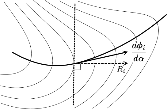
Figure 1: A two-dimensional model of the functional space. The thin solid lines denote the contours of the action $S$. The thick solid line is the valley line. The direction of the gradient vector $R_{i}$ and the tangent vector $d\phi_{i}/d\alpha$ are denoted by the arrows. The vertical dotted line is the subspace for the one-loop integral.

Substituting (2.5) into the path integral for the vacuum-to-vacuum transition amplitude,

$$Z={\cal N}\int\prod_{j}d\phi_{j}\ e^{-S},$$ (2.7)

we obtain

$$Z={\cal N}\int d\alpha\int\prod_{j}d\phi_{j}\delta\Bigl{(}(\phi_{i}-\phi_{i}(\alpha))R_{i}\Bigr{)}\left|{d\phi_{i}\over d\alpha}R_{i}\right|e^{-S(\phi)}.$$ (2.8)

The second (functional) integration, $\int\prod_{j}d\phi_{j}\delta((\phi_{i}-\phi_{i}(\alpha))R_{i})$, corresponds to the integration in the subspace denoted by the dotted line in Fig.1. At the one-loop order, the $\phi_{i}$ integration yields $\det^{\prime}$, the determinant of $D_{ij}$ restricted to the subspace. This subspace is orthogonal to the gradient vector, which is the eigenvector with the smallest eigenvalue $\lambda$ according to the new valley equation (2.1). Therefore this subspace is the whole space less the direction of the smallest eigenvalue of $D_{ij}$. Therefore the resulting determinant is simply the ordinary determinant less the smallest eigenvalue $\lambda$;

$${\rm det}^{\prime}={\det\over\lambda}_{\displaystyle.}$$ (2.9)

We thus obtain the following expression at the one-loop order;

$$Z={\cal N}^{\prime}\int d\alpha\left|{d\phi_{i}\over d\alpha}R_{i}\right|{1\over\sqrt{\det^{\prime}}}\ e^{-S(\phi(\alpha))}.$$ (2.10)

In this sense, the new valley method converts the smallest eigenvalue to the collective coordinate. This exact conversion is quite ideal for the actual calculation in the following sense: In physical situation one often suffers from a negative, zero, or positive but very small eigenvalue, which renders the ordinary Gaussian integration meaningless or unreliable. The new valley method saves this situation by converting the unwanted eigenvalue to the collective coordinate. The factor $\det^{\prime}$ is exactly free from this eigenvalue. An added bonus to this property is that the resulting det^′ is quite easy to calculate; we simply calculate the whole determinant and divide it by the smallest eigenvalue. If several unwanted eigenvalues exist, the new valley method can be extended straightforwardly. The equation should then specify that the gradient vector $\partial_{i}S$ lie in the subspace of the unwanted eigenvalues. This leads to a multi-dimensional valley with all the advantages noted above.

There is another valley method, called “streamline method” [17], which has been extensively used in the literatures. It proposes to trace the steepest descent line starting from a region of larger action. By this definition, its Jacobian is trivial at the one-loop order. Nevertheless, its subspace for the perturbative calculation has no relation to the eigenvalues of $D_{ij}$. Therefore, the determinant is not guaranteed to be free from the unwanted eigenvalue(s). Another problem is that it is a flow equation in the functional space: Since it is not a local definition in the functional space, it does not define any field equation. Therefore the construction of the configurations on the valley trajectory is quite difficult. Another problem is that it suffers from instability if the valley is traced from the bottom of the valley. This is not an issue for the problem of the instanton and anti-instanton valley, for which the higher end of the valley is known to be the pair separated by infinite distance. Yet this instability makes the streamline method useless for the current problem, for we only know the bottom of the valley, the zero-size instanton. For more detailed comparison of these methods and other features of the new valley method, we refer the readers to Ref.[20].

Let us discuss a toy model in a two-dimensional functional space, to show the power of the new valley method. The two degrees of freedom in the model is denoted as $\phi_{i}$ ($i=1,2$), and the action is given by the following,

$$S(\phi_{1},\phi_{2})={1\over g^{2}}\left((\phi_{1}^{2}+\phi_{2})^{2}+5(\phi_{1}^{2}-\phi_{2})^{2}\right)_{\displaystyle.}$$ (2.11)

This is constructed by distorting a simple parabolic potential so that the valley trajectory is not trivial. The new valley equation is now a simple algebraic equation, which can be solved numerically. Alternatively, we could reparametrize the functional space by $(r,\theta)$ defined by the following;

$$\phi_{1}^{2}+\phi_{2}=r\cos\theta,\hskip 8.53581pt\phi_{1}^{2}-\phi_{2}={1\over\sqrt{5}}r\sin\theta.$$ (2.12)

Under this parametrization $S=r^{2}/g^{2}$. Therefore following the variational interpretation of the new valley equation, we can minimize the square of the norm of the gradient vector, $(\partial_{i}S)^{2}$, as a function of $\theta$. In Fig.2, the thin lines denote the $S=$ constant lines, and the thick solid line denotes the new valley trajectory.

As an analogue of the constrained instanton formalism in this toy model, we introduce a simple constraint. Near the origin the valley trajectory extends to the $\phi_{1}$ direction. Any reasonable constraint has to reproduce this property. Therefore, as a simple example for the constraint, we choose the following;

$$\phi_{1}={\rm const.}$$ (2.13)

The solution of the constraint method is plotted in Fig.2 by the dashed line.

In Fig.2, it is apparent that the new valley trajectory goes through the region of importance, while the constrained trajectory does not. This property can be displayed more explicitly by considering the analogue of the physical observables $O(p,q)$ defined by the following;

$$O(p,q)=\int_{0}^{\infty}d\phi_{1}\int_{-\infty}^{\infty}d\phi_{2}\ \phi_{1}^{p}\phi_{2}^{q}\ e^{-S(\phi_{1},\phi_{2})}.$$ (2.14)

Following the prescription given above, we have carried out the numerical evaluation of $O(p,q)$ exactly and by the Gaussian (“one-loop”) approximation around the new valley trajectory and the constrained trajectory. Table.1 gives the ratio of the one-loop values over the exact value.

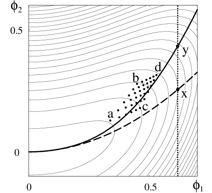
Figure 2: The valley instanton and the constrained instanton in the toy model. The solid line denotes the valley instanton and the dashed line shows the constrained instanton. The dots show the positions of the saddle points of the integrand of $O(p,q)$.

As is seen in the table, the new valley method gives a better approximation than the constraint method in this range of $(p,q)$ consistently. This could be explained in the following manner; one could calculate the position of the maximum of the integrand in (2.14), or the following “effective action”;

$$\tilde{S}^{(p,q)}(\phi)=S(\phi)-p\log\phi_{1}-q\log\phi_{2}.$$ (2.15)

The peak positions calculated in this manner are denoted in Fig.2 by dots. The point $a$ in the left bottom is for $(p,q)=(2,2)$, $b$ for $(2,12)$, $c$ for $(12,2)$, and $d$ for $(12,12)$. The dots are distributed around the new valley trajectory. This explains the fact that the new valley trajectory gives the better approximation over the constrained trajectory. Only when the power of one of the observable gets high enough as in the point $c$, the constraint method starts to give a little better values. However, this is exactly the range in which the ordinary instanton calculation starts to fail; For the $n$-point function with $n>O(1/g^{2})$, it is well known that one needs to take into account the effect of the external particles on the instanton itself. The power of the valley method lies in the fact that even in this range the calculation is done with good accuracy for generic type of observables, like the (12,12) case. Only when the observable is very special, like the (12,2) case, the constraint method tuned to that operator may give reasonable estimates.

$p\backslash q$	2	4	$6$	8	10	12
2	0.827	0.679	0.585	0.520	0.474	0.439
	0.545	0.248	0.110	0.049	0.022	0.010
4	0.997	0.870	0.767	0.689	0.629	0.581
	0.667	0.324	0.149	0.068	0.030	0.014
6	1.061	0.986	0.900	0.826	0.764	0.712
	0.737	0.384	0.185	0.086	0.040	0.018
8	1.064	1.046	0.991	0.931	0.876	0.826
	0.783	0.432	0.218	0.105	0.050	0.023
10	1.029	1.063	1.041	1.003	0.960	0.918
	0.815	0.473	0.248	0.123	0.060	0.028
12	0.971	1.046	1.058	1.043	1.017	0.985
	0.839	0.508	0.276	0.141	0.070	0.034

Table 1: The ratio of the $O(p,q)$ estimated by new valley method (the upper column) and the constraint method (the lower column) over the exact value for $g=0.2$.

Let us note a tricky point in comparing the valley instanton and the constrained instanton. If we compare them with the same parameter values, the constrained instanton has smaller action than the valley instanton. This is not a contradiction, nor it means the constrained instanton has a larger contribution: This becomes clear by considering the dotted vertical line in Fig.2. The point $x$ and $y$ are the valley and the constrained configurations, respectively, which have the same value of $\phi_{1}$. The configuration $y$ has a larger action than $x$, by the definition of the constraint method. However, as we have seen above, this does not mean that the constrained trajectory gives a better approximation. (One way to illustrate this point is that if we compare the configurations at the same distance, $\int d\alpha|(d\phi_{i}/d\alpha)R_{i}|$, from the origin, the valley configuration has the smaller action.) The same situation will be seen in the results of the following sections; when we compare the instantons at the same value of the constraint parameter, the constrained instanton has a smaller action than that of the valley instanton. This is a red herring and has nothing to do with the relevancy of the valley instanton.

In this analysis we took a very simple constraint (2.13). Alternatively we could take some ad-hoc constraint as long as any of these yield “finite-size” instantons, i.e., points away from the origin. Most of these constraints yield essentially similar results. Only when the trajectory goes through the dotted area in the Fig.1, one can obtain good quantitative results. Such a trajectory, however, is destined to be very close to the new valley trajectory. Therefore the new valley method, defined without any room for adjustment and guaranteed to give good results is superior to the constrained method.

Finally, we note that in the actual calculation of the solutions in the continuum space-time it is useful to introduce an auxiliary field. Let us denote all the real bosonic fields in the theory by $\phi_{\alpha}(x)$. We introduce the auxiliary field $F_{\alpha}(x)$ for each bosonic field and write the new valley equation as follows;

$$\sum_{\beta}\int d^{4}y{\delta^{2}S\over\delta\phi_{\alpha}(x)\delta\phi_{\beta}(y)}F_{\beta}(y)=\lambda F_{\alpha}(x),\hskip 11.38109ptF_{\alpha}(x)={\delta S\over\delta\phi_{\alpha}(x)}_{\displaystyle.}$$ (2.16)

This is a set of second-order differential equation, which can be analyzed by the conventional methods. The solution of the ordinary field equation of motion is a solution of (2.16) with $F_{\alpha}(x)=0$. In other words, $F_{\alpha}(x)$ specifies where and how much the valley configuration deviates from the solution of equation of motion. This property is useful for the qualitative discussion of the properties of the valley configurations. The analysis in the following sections will be carried out in this auxiliary field formalism (2.16).

3 The scalar $\phi^{4}$ field theory

We consider the scalar $\phi_{4}^{4}$ theory with Euclidean Lagrangian,

$${\cal L}=\frac{1}{g^{2}}\left[\frac{1}{2}(\partial_{\mu}\phi)^{2}+\frac{1}{2}\mu^{2}\phi^{2}-\frac{1}{4!}\phi^{4}\right].$$ (3.1)

The negative sign for the $\phi^{4}$ term is relevant for performing the asymptotic estimate in the theory with a positive $\phi^{4}$ term [11, 12, 13, 14, 15]. This model allows finite-size instantons only for $\mu=0$; otherwise, a simple scaling argument shows that the action of any finite-size configuration can be reduced by reducing its size.

3.1 Valley instanton

For this model, the new valley equation introduced in the previous section is

$$\begin{array}[]{cc}&\displaystyle-\partial_{\mu}\partial_{\mu}\phi+\mu^{2}\phi-\frac{1}{3!}\phi^{3}=F,\\[14.22636pt] &\displaystyle\left(-\partial_{\mu}\partial_{\mu}+\mu^{2}-\frac{1}{2}\phi^{2}\right)F=\lambda F.\end{array}$$ (3.4)

Now we introduce the scale parameter $\rho$ defined by $\phi(0)\equiv 4\sqrt{3}/\rho$, in order to fix the radius of the instanton solution to be unity. We rescale fields and variables as in the following;

$$r=\frac{\sqrt{x^{2}}}{\rho},\quad\lambda=\mu^{2}\nu,\quad\phi(x)=\frac{h(r)}{\rho},\quad F(x)=\frac{\mu^{2}}{\rho}f(r).$$ (3.5)

The new valley equation (3.4) is given by the following under this rescaling;

$$-\frac{1}{r^{3}}\frac{d}{dr}\left(r^{3}\frac{dh}{dr}\right)+(\rho\mu)^{2}h-\frac{1}{3!}h^{3}=(\rho\mu)^{2}f,$$ (3.6)

$$-\frac{1}{r^{3}}\frac{d}{dr}\left(r^{3}\frac{df}{dr}\right)+(\rho\mu)^{2}f-\frac{1}{2}h^{2}f=(\rho\mu)^{2}\nu f.$$ (3.7)

This system has an instanton solution in the massless limit, $\rho\mu\to 0$ [11, 12]. In this limit, (3.6) reduces to the equation of motion and (3.7) the equation for the zero-mode fluctuation, $f$, around the instanton solution. The solution is the following;

$$\begin{array}[]{cc}\displaystyle h_{0}=\frac{4\sqrt{3}}{1+r^{2}},&\displaystyle f_{0}=C\left(\frac{4\sqrt{3}}{1+r^{2}}-\frac{8\sqrt{3}}{(1+r^{2})^{2}}\right),\end{array}$$ (3.9)

where $C$ is an arbitrary constant. Note that solution $f_{0}$ is obtained from $\partial\phi_{0}(x)/\partial\rho$, $\phi_{0}=h_{0}/\rho$.

Let us construct the valley instanton in the scalar $\phi^{4}$ theory analytically. When $\rho\mu$ is very small but finite, the valley instanton is expected to have $\rho\mu$ corrections to (3.9). On the other hand, at large distance from the core region of the valley instanton, since the term of $O(h^{2})$ is negligible, the valley equation can be linearized. This linearized equation can be solved easily. By matching the solution near the core and the solution in the asymptotic region in the overlapping intermediate region, we can construct approximate solution analytically. We will carry out this procedure in the following.

In the asymptotic region, $(\rho\mu)^{2}\gg h^{2}$, the linearized valley equation is the following;

$$\begin{array}[]{cc}&\displaystyle-\frac{1}{r^{3}}\frac{d}{dr}\left(r^{3}\frac{dh}{dr}\right)+(\rho\mu)^{2}h=(\rho\mu)^{2}f,\\[14.22636pt] &\displaystyle-\frac{1}{r^{3}}\frac{d}{dr}\left(r^{3}\frac{df}{dr}\right)+(\rho\mu)^{2}f=(\rho\mu)^{2}\nu f.\end{array}$$ (3.12)

The solution of these equations is

$$h(r)=C_{1}G_{\rho\mu}(r)+\frac{f}{\nu},\quad f(r)=C_{2}G_{\rho\mu\sqrt{1-\nu}}(r),$$ (3.13)

where $C_{1}$ and $C_{2}$ are arbitrary functions of $\rho\mu$. The function $G_{m}(r)$ is

$$G_{m}(r)=\frac{mK_{1}(mr)}{(2\pi)^{2}r},$$ (3.14)

where $K_{1}$ is a modified Bessel function. The functions $f$ and $h$ decay exponentially at large $r$. In the region of $r\ll(\rho\mu)^{-1}$, $r\ll(\rho\mu\sqrt{1-\nu})^{-1}$, $f$ and $h$ can be expanded in series as the following;

$$\begin{array}[]{lll}&\displaystyle h=\frac{C_{1}}{(2\pi)^{2}}\left[\frac{1}{r^{2}}+\frac{1}{2}(\rho\mu)^{2}\ln(\rho\mu rc)+\cdots\right]\\[14.22636pt] &\displaystyle\hskip 7.3194pt+\frac{C_{2}}{(2\pi)^{2}\nu}\left[\frac{1}{r^{2}}+\frac{1}{2}(\rho\mu)^{2}(1-\nu)\ln(\rho\mu\sqrt{1-\nu}rc)+\cdots\right],\\[14.22636pt] &\displaystyle f=\frac{C_{2}}{(2\pi)^{2}}\left[\frac{1}{r^{2}}+\frac{1}{2}(\rho\mu)^{2}(1-\nu)\ln(\rho\mu\sqrt{1-\nu}rc)+\cdots\right].\end{array}$$ (3.18)

In the above, $c=e^{\gamma-1/2}/2$, where $\gamma$ is the Euler’s constant.

Near the origin, we expect that the valley instanton is similar to the ordinary instanton. It is convenient to define $\hat{h}$ and $\hat{f}$ as the following;

$$h=h_{0}+(\rho\mu)^{2}\hat{h},\qquad f=f_{0}+(\rho\mu)^{2}\hat{f},$$ (3.19)

where $C$ in $f_{0}$ is the function of $\rho\mu$ and is decided in the following. The “core region” is defined as

$$h_{0}\gg(\rho\mu)^{2}\hat{h},\qquad f_{0}\gg(\rho\mu)^{2}\hat{f}.$$ (3.20)

The valley equation for perturbation field $\hat{h}$, $\hat{f}$ becomes

$$\begin{array}[]{ll}&\displaystyle-\frac{1}{r^{3}}\frac{d}{dr}\left(r^{3}\frac{d\hat{h}}{dr}\right)-\frac{1}{2}h_{0}^{2}\hat{h}=f_{0}-h_{0},\\[14.22636pt] &\displaystyle-\frac{1}{r^{3}}\frac{d}{dr}\left(r^{3}\frac{d\hat{f}}{dr}\right)-\frac{1}{2}h_{0}^{2}\hat{f}=(\nu-1)f_{0}+h_{0}f_{0}\hat{h}.\end{array}$$ (3.23)

The left-hand side of (3.23) has a zero mode, $\varphi$. It satisfies the equation,

$$-\frac{1}{r^{3}}\frac{d}{dr}\left(r^{3}\frac{d\varphi}{dr}\right)-\frac{1}{2}h_{0}^{2}\,\varphi=0,$$ (3.24)

and is given by the following;

$$\varphi=\frac{4\sqrt{3}}{1+r^{2}}-\frac{8\sqrt{3}}{(1+r^{2})^{2}}.$$ (3.25)

We multiply $r^{3}\varphi$ to both sides of (3.23), and integrate them from $0$ to $r$. The existence of zero mode $\varphi$ makes it possible to integrate the left-hand side of (3.23). As a result of the integration by parts, only the surface terms remain and we obtain,

$$\displaystyle-r^{3}\varphi\frac{d\hat{h}}{dr}+r^{3}\frac{d\varphi}{dr}\hat{h}=\int_{0}^{r}dr^{\prime}r^{\prime 3}\varphi\left[f_{0}-h_{0}\right],$$ (3.26)

$$\displaystyle-r^{3}\varphi\frac{d\hat{f}}{dr}+r^{3}\frac{d\varphi}{dr}\hat{f}=\int_{0}^{r}dr^{\prime}r^{\prime 3}\varphi\left[(\nu-1)f_{0}+h_{0}f_{0}\hat{h}\right].$$ (3.27)

First, using (3.9) and (3.25), we can find that the right-hand side of (3.26) is proportional to $\ln r$ at $r\gg 1$. Thus (3.26) becomes

$$\displaystyle r\frac{d\hat{h}}{dr}+2\hat{h}=4\sqrt{3}\,(1-C)\ln r.$$ (3.28)

This equation can be solved easily at $r\gg 1$. Using the solution of (3.28), we can find the right-hand side of (3.26) also proportional to $\ln r$ as the following;

$$\displaystyle r\frac{d\hat{f}}{dr}+2\hat{f}=4\sqrt{3}\,C(1-\nu)\ln r.$$ (3.29)

Finally, we obtain $\hat{h}$ and $\hat{f}$ at $r\gg 1$,

$$\hat{h}=2\sqrt{3}\,(1-C)\ln r+\cdots,\quad\hat{f}=(1-\nu)2\sqrt{3}\,C\ln r+\cdots.$$ (3.30)

For these solutions to meet to (3.18), the parameters need to be the following;

$$C_{1}=0,\quad C_{2}=4\sqrt{3}\,(2\pi)^{2},\quad\nu=1,\quad C=1,$$ (3.31)

as $\rho\mu=0$. Now we have obtained the solution of the new valley equation;

$$h(r)=\left\{\begin{array}[]{ll}\displaystyle\frac{4\sqrt{3}}{1+r^{2}},&\quad\mbox{if}\quad r\ll(\rho\mu)^{-1/2};\\[11.38092pt] \displaystyle\frac{4\sqrt{3}}{r^{2}}+o\left((\rho\mu)^{2}\right),&\quad\mbox{if}\quad(\rho\mu)^{-1/2}\ll r\ll(\rho\mu)^{-1};\\[11.38092pt] \displaystyle 4\sqrt{3}\,(2\pi^{2})\,G_{\rho\mu\sqrt{1-\nu}}\,(r),&\quad\mbox{if}\quad(\rho\mu)^{-1/2}\ll r.\end{array}\right.$$ (3.32)

Let us discuss the consistency of our analysis. In the construction of the analytical solution, especially in the argument of the matching of the core and asymptotic region solution, we have implicitly assumed that there exists an overlapping region where both (3.12) and (3.23) are valid. Using the solution (3.32), it is found that (3.12) is valid in the region of $r\gg(\rho\mu)^{-1/2}$, and (3.23) is valid in the region of $r\ll(\rho\mu)^{-1}$. Therefore in the above analysis we have limited our calculation in the overlapping region $(\rho\mu)^{-1/2}\ll r\ll(\rho\mu)^{-1}$.

We calculate the action of the valley instanton using the above solution. Rewriting the action in terms of $h(r)$, we find

$$S=\frac{\pi^{2}}{g^{2}}\int_{0}^{\infty}dr\,r^{3}\left[\left(\frac{dh}{dr}\right)^{2}+(\rho\mu)^{2}h^{2}-\frac{1}{12}h^{4}\right].$$ (3.33)

Substituting the analytic solution for $S$, we obtain

$$S=\frac{16\pi^{2}}{g^{2}}+O\left((\rho\mu)^{2}\right).$$ (3.34)

The leading contribution term comes from the ordinary instanton solution, and the correction term comes from the distortion of the instanton solution.

3.2 Constrained instanton

In this subsection, we consider the constrained instanton in the scalar $\phi^{4}$ theory, following the construction in Ref.[15]. We require the constraint in the path integral. The field equation under the constraint is

$$\frac{\delta S}{\delta\phi}+\sigma\frac{\delta O}{\delta\phi}=0,$$ (3.35)

where $\sigma$ is a Lagrange multiplier. The functional $O$ had to satisfy the certain scaling properties that guarantee the existence of the solution [15]. We choose it as follows;

$$O=\int d^{4}x\,\frac{\phi^{6}}{6}.$$ (3.36)

This choice is one of the simplest for constructing the constrained instanton in the scalar $\phi^{4}$ theory. Again, adopting the rescaling (3.5), the equation of motion under this constraint becomes

$$-\frac{1}{r^{3}}\frac{d}{dr}\left(r^{3}\frac{dh}{dr}\right)+(\rho\mu)^{2}h-\frac{1}{3!}h^{3}+(\rho\mu)^{2}\tilde{\sigma}h^{5}=0,$$ (3.37)

where we rescale the parameter $\sigma$ as $\sigma=(\rho\mu)^{2}\widetilde{\sigma}$. The solution of this equation can be constructed in a manner similar to the previous section. To carry out the perturbation calculation in the core region, we replace the field variable as $h=h_{0}+(\rho\mu)^{2}\hat{h}$, where $h_{0}\gg(\rho\mu)^{2}\hat{h}$. The field equation of $\hat{h}$ becomes

$$-\frac{1}{r^{3}}\frac{d}{dr}\left(r^{3}\frac{d\hat{h}}{dr}\right)-\frac{1}{2}h_{0}^{2}\hat{h}=-h_{0}-\tilde{\sigma}h_{0}^{5}.$$ (3.38)

We multiply this equation by the zero mode (3.25) and integrate this from $0$ to $r$. Then we obtain

$$-r^{3}\varphi\frac{d\hat{h}}{dr}+r^{3}\frac{d\varphi}{dr}\hat{h}=-\int_{0}^{r}dr^{\prime}r^{\prime 3}\varphi\left[h_{0}+\tilde{\sigma}h_{0}^{5}\right].$$ (3.39)

The solution of this equation in the region where $r\gg 1$ is

$$\hat{h}=2\sqrt{3}\ln r-\frac{192\sqrt{3}}{7}\tilde{\sigma}+\cdots.$$ (3.40)

In the asymptotic region, we consider the field variable and the parameter as $h^{2}\ll(\rho\mu)^{2}$, $\widetilde{\sigma}h^{4}\ll 1$. Under this condition, the field equation of the asymptotic region becomes

$$-\frac{1}{r^{3}}\frac{d}{dr}\left(r^{3}\frac{dh}{dr}\right)+(\rho\mu)^{2}h=0.$$ (3.41)

The solution is

$$h(r)=C_{1}G_{\rho\mu}(r),$$ (3.42)

where $C_{1}$ is arbitrary constant. In the region of $r\ll(\rho\mu)^{-1}$, this solution can be expanded as the following;

$$h=\frac{C_{1}}{(2\pi)^{2}}\left[\frac{1}{r^{2}}+\frac{1}{2}(\rho\mu)^{2}\ln(\rho\mu rc)+\cdots\right].$$ (3.43)

Matching this solution and the core region solution (3.40), parameters are determined as the following;

$$C_{1}=4\sqrt{3}(2\pi)^{2},\quad\tilde{\sigma}=-\frac{7}{96}\ln(\rho\mu).$$ (3.44)

To summarize, the analytical solution of the constrained instanton we have obtained is the following,

$$h(r)=\left\{\begin{array}[]{ll}\displaystyle\frac{4\sqrt{3}}{1+r^{2}},&\quad\mbox{if}\quad r\ll(\rho\mu)^{-1/2};\\[11.38092pt] \displaystyle\frac{4\sqrt{3}}{r^{2}}+2\sqrt{3}(\rho\mu)^{2}\ln(\rho\mu rc)+o\left((\rho\mu)^{2}\right),&\quad\mbox{if}\quad(\rho\mu)^{-1/2}\ll r\ll(\rho\mu)^{-1};\\[11.38092pt] \displaystyle 4\sqrt{3}\,(2\pi^{2})\,G_{\rho\mu}\,(r),&\quad\mbox{if}\quad(\rho\mu)^{-1/2}\ll r.\end{array}\right.$$ (3.45)

The action of the constrained instanton is given by the following;

$$S=\frac{16\pi^{2}}{g^{2}}-96\pi^{2}(\rho\mu)^{2}\ln(\rho\mu)+O\left((\rho\mu)^{2}\right).$$ (3.46)

This differs from the action of the valley instanton at the next-to-leading order. This correction term shows that the constrained instanton is more distorted from the ordinary instanton than the valley instanton.

3.3 Numerical analysis

In this subsection, we calculate the valley equation (3.6), (3.7) and the constrained equation (3.37) numerically. Then we compare the valley and the constraint instanton.

Each of the equations is the second order differential equation, so we require two boundary conditions for each field variable to decide the solution. We require all the field variables are regular at the origin. The finiteness of the action requires $h,f\to 0$ faster than $1/r^{2}$ at infinity. In solving (3.6) and (3.7), we adjust the parameter $\nu$ and $f(0)$ so that $h,f\to 0$ at infinity for the fixed $\rho\mu$. In the similar way, in case of the constrained instanton, the parameter $\sigma$ is determined so that $h\to 0$ at infinity.

Numerical solutions of the valley equation near the origin are plotted in Fig.3 (a) for $\rho\mu=0.1,\,1.0$. The solid line shows the instanton solutions (3.9), which corresponds to $\rho\mu=0$. The numerical solutions of the constrained instanton are also plotted in Fig.3 (b) for $\rho\mu=0.1,\,0.5,\,1.0$. Both the valley and the constraint solution for $\rho\mu=0.1$ agree with the analytical result. As $\rho\mu$ becomes large, both solutions are deformed from the original instanton solution. We find that the distortion of the constrained instanton is much larger than that of the valley instanton. This also agrees with the analytic result. In the analytical solution (3.45), the correction term $2\sqrt{3}(\rho\mu)^{2}\ln(\rho\mu rc)$ contributes to this distortion. On the other hand, the correction term of the valley instanton (3.45) is $o\left((\rho\mu)^{2}\right)$, which is smaller than the previous one. In addition, we find that the exponentially damping behavior of the analytical solution in the asymptotic region, where $r\gg(\rho\mu)^{-1}$ agrees with the result of numerical analysis.

Figure 3: (a) Shapes of the numerical solution of the valley instanton, $h(r)$, for $\rho\mu=$$0,$ $0.1,$ and $1.0$ near the origin. The solid line denotes the original instanton, $h_{0}$. (b) Shapes of the constrained instanton for $\rho\mu=$$0,$ $0.1,$ $0.5,$ and $1.0$.

The values of the action of the valley instanton for $\rho\mu=$$0.0001\sim 1.0$ are plotted in Fig.4 (a). If $\rho\mu$ is very small, this result is consistent with (3.34). The values of the action of the constrained instanton for $\rho\mu=$ $0.0001\sim 0.8$ are plotted in Fig.4 (b). This figure shows that the behavior of the action is similar to that of the valley instanton when $\rho\mu$ is very small. When $\rho\mu$ becomes large, the behavior of the action is different from the valley instanton case.

We summarize all the numerical data in the Table 2.

Figure 4: (a) The action $S$ (in units of $g^{2}/16\pi^{2}$) of the numerical solution of the valley equation as a function of the parameter $\rho\mu$. (b) The action $S$ of the constrained instanton.

	valley instanton			constrained instanton
$\rho\mu$	$\nu$	$f(0)$	$g^{2}S/16\pi^{2}$	$\sigma$	$g^{2}S/16\pi^{2}$
0.0001	0.971	-7.14	1.000002	0.000000079	1.000008
0.001	0.958	-7.21	1.000021	0.000000394	1.000021
0.01	0.940	-7.44	1.001585	0.000019342	1.001281
0.05	0.917	-7.93	1.035008	0.000257518	1.019044
0.1	0.901	-8.43	1.092489	0.000661283	1.055766
0.2	0.876	-9.40	1.293706	0.001437910	1.148013
0.3	0.855	-10.41	1.571073	0.002055520	1.262493
0.4	0.833	-11.46	1.906408	0.002508380	1.259776
0.5	0.811	-12.57	2.282639	0.002817690	1.132618
0.6	0.787	-13.71	2.693832	0.003008290	0.616666
0.7	0.762	-14.87	3.134111	0.003104190	-0.867477
0.8	0.736	-16.01	3.574478	0.003127540	-4.848880
0.9	0.709	-17.12	4.047787	0.003098220	-15.87237
1.0	0.682	-18.18	4.550929	0.003033310	-49.97363

Table 2: The numerical data of the valley instanton and the constrained instanton in the scalar theory.

4 The gauge-Higgs system

We consider the SU(2) gauge theory with one scalar Higgs doublet, which has the following action $S=S_{g}+S_{h}$;

$$S_{g}=\frac{1}{2g^{2}}\int d^{4}x\ {\rm tr}F_{\mu\nu}F_{\mu\nu},$$ (4.1)

$$S_{h}=\frac{1}{\lambda}\int d^{4}x\left\{\left(D_{\mu}H\right)^{\dagger}\left(D_{\mu}H\right)+\frac{1}{8}\left(H^{\dagger}H-v^{2}\right)^{2}\right\},$$ (4.2)

where $F_{\mu\nu}=\partial_{\mu}A_{\nu}-\partial_{\nu}A_{\mu}-i\left[A_{\mu},A_{\nu}\right]$ and $D_{\mu}=\partial_{\mu}-iA_{\mu}$. The masses of the gauge boson and the Higgs boson are given by,

$$m_{{}_{W}}=\sqrt{\frac{g^{2}}{2\lambda}}v,\quad m_{{}_{H}}=\frac{1}{\sqrt{2}}v.$$ (4.3)

This theory is known not to have any finite-size instanton solutions, in spite of its importance. In this section, we will construct instanton-like configurations for this theory, relevant for tunneling phenomena, including the baryon and lepton number violation processes.

4.1 Valley instanton

The valley equation for this system is given by,

$$\frac{\delta^{2}S}{\delta A_{\mu}\delta A_{\nu}}F^{A}_{\nu}+\frac{\delta^{2}S}{\delta A_{\mu}\delta H^{\dagger}}F^{H}+\frac{\delta^{2}S}{\delta A_{\mu}\delta H}F^{H\dagger}=\lambda_{e}F^{A}_{\mu},$$

$$\frac{\delta^{2}S}{\delta H^{\dagger}\delta A_{\mu}}F^{A}_{\mu}+\frac{\delta^{2}S}{\delta H^{\dagger}\delta H}F^{H\dagger}+\frac{\delta^{2}S}{\delta H^{\dagger}\delta H^{\dagger}}F^{H}=\lambda_{e}F^{H\dagger},$$ (4.4)

$$F^{A}_{\mu}=\frac{\delta S}{\delta A_{\mu}},\quad F^{H}=\frac{\delta S}{\delta H},$$

where the integration over the space-time is implicit. The valley is parametrized by the eigenvalue $\lambda_{e}$ that is identified with the zero mode corresponding to the scale invariance in the massless limit, $v\rightarrow 0$.

To simplify the equation, we adopt the following ansatz;

$$A_{\mu}(x)=\frac{x_{\nu}\bar{\sigma}_{\mu\nu}}{x^{2}}\cdot 2a(r),\quad H(x)=v\left(1-h(r)\right)\eta,$$ (4.5)

where $\eta$ is a constant isospinor, and $a$ and $h$ are real dimensionless functions of dimensionless variable $r$, which is defined by $r=\sqrt{x^{2}}/\rho$. The matrix $\bar{\sigma}_{\mu\nu}$ is defined, according to the conventions of Ref.[9], as $\bar{\sigma}_{\mu\nu}=\bar{\eta}_{a\mu\nu}\sigma^{a}/2$. We have introduced the scaling parameter $\rho$ so that we adjust the radius of valley instanton as we will see later in subsection 4.3. The tensor structure in (4.5) is the same as that of the instanton in the singular gauge [5].

Inserting this ansatz to (4.4), the structure of $F^{A}_{\mu}$ and $F^{H\dagger}$ is determined as the following;

$$F^{A}_{\mu}(x)=\frac{x_{\nu}\bar{\sigma}_{\mu\nu}}{x^{2}}\cdot\frac{2v^{2}}{\lambda}f^{a}(r), F^{H\dagger}(x)=-\frac{v^{3}}{\lambda}f^{h}(r)\eta.$$ (4.6)

By using this ansatz, (4.5) and (4.6), the valley equation (4.4) is reduced to the following;

$$-\frac{1}{r}\frac{d}{dr}\left(r\frac{da}{dr}\right)+\frac{4}{r^{2}}a(a-1)(2a-1)+\frac{g^{2}}{2\lambda}(\rho v)^{2}a(1-h)^{2}=\frac{g^{2}}{\lambda}(\rho v)^{2}f^{a},$$ (4.7)

$$-\frac{1}{r^{3}}\frac{d}{dr}\left(r^{3}\frac{dh}{dr}\right)+\frac{3}{r^{2}}(h-1)a^{2}+\frac{1}{4}(\rho v)^{2}h(h-1)(h-2)=(\rho v)^{2}f^{h},$$ (4.8)

$$-\frac{1}{r}\frac{d}{dr}\left(r\frac{df^{a}}{dr}\right)+\frac{4}{r^{2}}(6a^{2}-6a+1)f^{a}+\frac{g^{2}}{2\lambda}(\rho v)^{2}(h-1)^{2}f^{a}$$

$$\hskip 129.16626pt+\frac{g^{2}}{\lambda}(\rho v)^{2}a(h-1)f^{h}=\frac{g^{2}}{\lambda}(\rho v)^{2}\nu f^{a},$$ (4.9)

$$-\frac{1}{r^{3}}\frac{d}{dr}\left(r^{3}\frac{df^{h}}{dr}\right)+\frac{3a^{2}}{r^{2}}f^{h}+\frac{1}{4}(\rho v)^{2}(3h^{2}-6h+2)f^{h}$$

$$\hskip 129.16626pt+\frac{6a}{r^{2}}(h-1)f^{a}=(\rho v)^{2}\nu f^{h},$$ (4.10)

where $\nu$ is defined as $\lambda_{e}=v^{2}\nu/\lambda$.

In the massless limit, $\rho v\rightarrow 0$, (4.7) and (4.8) reduce to the equation of motion and (4.9) and (4.10) to the equation for the zero-mode fluctuation around the instanton solution. The solution of this set of equations is the following;

$$\begin{array}[]{cc}\displaystyle a_{0}=\frac{1}{1+r^{2}},&\displaystyle h_{0}=1-\left(\frac{r^{2}}{1+r^{2}}\right)^{1/2},\\[11.38109pt] \displaystyle f^{a}_{0}=\frac{2Cr^{2}}{(1+r^{2})^{2}},&\displaystyle f^{h}_{0}=\frac{Cr}{(1+r^{2})^{3/2}},\end{array}$$ (4.13)

where $C$ is an arbitrary function of $\rho v$. Note that $a_{0}$ is an instanton solution in the singular gauge and $h_{0}$ is a Higgs configuration in the instanton background [5]. We have adjusted the scaling parameter $\rho$ so that the radius of the instanton solution is unity. The mode solutions $f^{a}_{0}$ and $f^{h}_{0}$ are obtained from $\partial a_{0}/\partial\rho$ and $\partial h_{0}/\partial\rho$, respectively.

Now we will construct the valley instanton analytically. When $\rho v=0$, it is given by the ordinary instanton configuration $a_{0}$, $h_{0}$, $f^{a}_{0}$ and $f^{h}_{0}$. When $\rho v$ is small but not zero, it is expected that small $\rho v$ corrections appear in the solution. On the other hand, at large distance from the core of the valley instanton, this solution is expected to decay exponentially, because gauge boson and Higgs boson are massive. Therefore, the solution is similar to the instanton near the origin and decays exponentially in the asymptotic region. In the following, we will solve the valley equation in both regions and analyze the connection in the intermediate region. In this manner we will find the solution.

In the asymptotic region, $a$, $h$, $f^{a}$ and $f^{h}$ become small and the valley equation can be linearized;

$$-\frac{1}{r}\frac{d}{dr}\left(r\frac{da}{dr}\right)+\frac{4}{r^{2}}a+\frac{g^{2}}{2\lambda}(\rho v)^{2}a=\frac{g^{2}}{\lambda}(\rho v)^{2}f^{a},$$ (4.14)

$$-\frac{1}{r^{3}}\frac{d}{dr}\left(r^{3}\frac{dh}{dr}\right)+\frac{1}{2}(\rho v)^{2}h=(\rho v)^{2}f^{h},$$ (4.15)

$$-\frac{1}{r}\frac{d}{dr}\left(r\frac{df^{a}}{dr}\right)+\frac{4}{r^{2}}f^{a}+\frac{g^{2}}{2\lambda}(\rho v)^{2}f^{a}=\frac{g^{2}}{\lambda}(\rho v)^{2}\nu f^{h},$$ (4.16)

$$-\frac{1}{r^{3}}\frac{d}{dr}\left(r^{3}\frac{df^{h}}{dr}\right)+\frac{1}{2}(\rho v)^{2}f^{h}=(\rho v)^{2}\nu f^{h}.$$ (4.17)

The solution of this set of equations is

$$a(r)=C_{1}\,r\frac{d}{dr}G_{\rho m_{{}_{W}}}(r)+\frac{1}{\nu}f^{a}(r),$$ (4.18)

$$h(r)=C_{2}\,G_{\rho m_{{}_{H}}}(r)+\frac{1}{\nu}f^{h}(r),$$ (4.19)

$$f^{a}(r)=C_{3}\,r\frac{d}{dr}G_{\rho\mu_{{}_{W}}}(r),$$ (4.20)

$$f^{h}(r)=C_{4}\,G_{\rho\mu_{{}_{H}}}(r),$$ (4.21)

where $C_{i}$ are arbitrary functions of $\rho v$ and $\mu_{{}_{W,\,H}}$ are defined as $\mu_{{}_{W,\,H}}=m_{{}_{W,\,H}}\sqrt{1-2\nu}$. As was expected above, these solutions decay exponentially at infinity and when $r\ll(\rho v)^{-1}$ they have the series expansions;

$$a(r)=\frac{C_{1}}{(2\pi)^{2}}\left[-\frac{2}{r^{2}}+\frac{1}{2}(\rho m_{{}_{W}})^{2}+\cdots\right]+\frac{C_{3}}{\nu(2\pi)^{2}}\left[-\frac{2}{r^{2}}+\frac{1}{2}(\rho\mu_{{}_{W}})^{2}+\cdots\right],$$ (4.22)

$$h(r)=\frac{C_{2}}{(2\pi)^{2}}\left[\frac{1}{r^{2}}+\frac{1}{2}(\rho m_{{}_{H}})^{2}\ln(\rho m_{{}_{H}}rc)+\cdots\right]$$

$$\hskip 129.16626pt+\frac{C_{4}}{\nu(2\pi)^{2}}\left[\frac{1}{r^{2}}+\frac{1}{2}(\rho\mu_{{}_{H}})^{2}\ln(\rho\mu_{{}_{H}}rc)+\cdots\right],$$ (4.23)

$$f^{a}(r)=\frac{C_{3}}{(2\pi)^{2}}\left[-\frac{2}{r^{2}}+\frac{1}{2}(\rho\mu_{{}_{W}})^{2}+\cdots\right],$$ (4.24)

$$f^{h}(r)=\frac{C_{4}}{(2\pi)^{2}}\left[\frac{1}{r^{2}}+\frac{1}{2}(\rho\mu_{{}_{H}})^{2}\ln(\rho\mu_{{}_{H}}rc)+\cdots\right],$$ (4.25)

$c$ being a numerical constant $e^{\gamma-1/2}/2$, where $\gamma$ is the Euler’s constant.

Near the origin, we expect that the valley instanton is similar to the ordinary instanton. Then the following replacement of the field variables is convenient; $a=a_{0}+(\rho v)^{2}\hat{a}$, $h=h_{0}+(\rho v)^{2}\hat{h}$, $f^{a}=f^{a}_{0}+(\rho v)^{2}\hat{f^{a}}$, $f^{h}=f^{h}_{0}+(\rho v)^{2}\hat{f^{h}}$. If we assume $a_{0}\gg(\rho v)^{2}\hat{a}$, $h_{0}\gg(\rho v)^{2}\hat{h}$, $f^{a}_{0}\gg(\rho v)^{2}\hat{f^{a}}$ and $f^{h}_{0}\gg(\rho v)^{2}\hat{f^{h}}$, the valley equation becomes

$$-\frac{1}{r}\frac{d}{dr}\left(r\frac{d\hat{a}}{dr}\right)+\frac{4}{r^{2}}(6a_{0}^{2}-6a_{0}+1)\hat{a}+\frac{g^{2}}{2\lambda}a_{0}(h_{0}-1)^{2}=\frac{g^{2}}{\lambda}f^{a}_{0},$$ (4.26)

$$-\frac{1}{r^{3}}\frac{d}{dr}\left(r^{3}\frac{d\hat{h}}{dr}\right)+\frac{3}{r^{2}}a_{0}^{2}\hat{h}+\frac{6}{r^{2}}(h_{0}-1)a_{0}\hat{a}+\frac{1}{4}h_{0}(h_{0}-1)(h_{0}-2)=f^{h}_{0},$$ (4.27)

$$-\frac{1}{r}\frac{d}{dr}\left(r\frac{d\hat{f^{a}}}{dr}\right)+\frac{4}{r^{2}}(6a_{0}^{2}-6a_{0}+1)\hat{f^{a}}+\frac{24}{r^{2}}(2a_{0}-1)f^{a}_{0}\hat{a}$$

$$\hskip 120.55518pt+\frac{g^{2}}{2\lambda}(h_{0}-1)^{2}f^{a}_{0}+\frac{g^{2}}{\lambda}a_{0}(h_{0}-1)f^{h}_{0}=\frac{g^{2}}{\lambda}\nu f^{a}_{0},$$ (4.28)

$$-\frac{1}{r^{3}}\frac{d}{dr}\left(r^{3}\frac{d\hat{f^{h}}}{dr}\right)+\frac{3}{r^{2}}a_{0}^{2}\hat{f^{h}}+\frac{6}{r^{2}}a_{0}f^{h}_{0}\hat{a}+\frac{1}{4}(3h_{0}^{2}-6h_{0}+2)f^{h}_{0}$$

$$\hskip 86.11084pt+\frac{6}{r^{2}}a_{0}(h_{0}-1)\hat{f^{a}}+\frac{6}{r^{2}}(h_{0}-1)f^{a}_{0}\hat{a}+\frac{6}{r^{2}}a_{0}f^{a}_{0}\hat{h}=\nu f^{h}_{0}.$$ (4.29)

To solve this equation, we introduce solutions of the following equations;

$$\begin{array}[]{l}\displaystyle-\frac{1}{r}\frac{d}{dr}\left(r\frac{d\varphi_{a}}{dr}\right)+\frac{4}{r^{2}}(6a_{0}^{2}-6a_{0}+1)\varphi_{a}=0,\\ \\ \displaystyle-\frac{1}{r^{3}}\frac{d}{dr}\left(r^{3}\frac{d\varphi_{h}}{dr}\right)+\frac{3}{r^{2}}a_{0}^{2}\varphi_{h}=0.\end{array}$$ (4.30)

They are given as,

$$\varphi_{a}=\frac{r^{2}}{(1+r^{2})^{2}},\quad\varphi_{h}=\left(\frac{r^{2}}{1+r^{2}}\right)^{1/2}.$$ (4.31)

Using these solutions, we will integrate the valley equation. We multiply (4.26) and (4.28) by $r\varphi_{a}$, and multiply (4.27) and (4.29) by $r^{3}\varphi_{h}$ then integrate them from $0$ to $r$. Integrating by parts and using (4.30), we obtain

$$-\varphi_{a}r\frac{d\hat{a}}{dr}+\frac{d\varphi_{a}}{dr}r\hat{a}=\frac{g^{2}}{\lambda}\int_{0}^{r}dr^{\prime}r^{\prime}\varphi_{a}\left[f^{a}_{0}-\frac{1}{2}a_{0}(h_{0}-1)^{2}\right],$$ (4.32)

$$-\varphi_{h}r^{3}\frac{d\hat{h}}{dr}+\hat{h}r^{3}\frac{d\varphi_{h}}{dr}=\int_{0}^{r}dr^{\prime}r^{\prime 3}\varphi_{h}\left[f^{h}_{0}-\frac{1}{4}h_{0}(h_{0}-1)(h_{0}-2)-\frac{6}{r^{\prime 2}}(h_{0}-1)a_{0}\hat{a}\right],$$

(4.33)

$$-\varphi_{a}r\frac{d\hat{f^{a}}}{dr}+\frac{d\varphi_{a}}{dr}r\hat{f^{a}}$$

$$\hskip 8.61108pt=\int_{0}^{r}dr^{\prime}r^{\prime}\varphi_{a}\left[\frac{g^{2}}{\lambda}\nu f^{a}_{0}-\frac{24}{r^{\prime 2}}(2a_{0}-1)f^{a}_{0}\hat{a}-\frac{g^{2}}{2\lambda}(h_{0}-1)^{2}f^{a}_{0}-\frac{g^{2}}{\lambda}a_{0}(h_{0}-1)f^{h}_{0}\right],$$ (4.34)

$$-\varphi_{h}r^{3}\frac{d\hat{f^{h}}}{dr}+\hat{h}r^{3}\frac{d\varphi_{h}}{dr}$$

$$\hskip 8.61108pt=\int_{0}^{r}dr^{\prime}r^{\prime 3}\varphi_{h}\left[\nu f^{h}_{0}-\frac{6}{r^{\prime 2}}a_{0}f^{a}_{0}\hat{a}-\frac{1}{4}(3h_{0}^{2}-6h_{0}+2)f^{h}_{0}\right.$$

$$\hskip 124.86072pt\left.-\frac{6}{r^{\prime 2}}a_{0}(h_{0}-1)\hat{f^{a}}-\frac{6}{r^{\prime 2}}(h_{0}-1)f^{a}_{0}\hat{a}-\frac{6}{r^{\prime 2}}a_{0}f^{a}_{0}\hat{h}\right].$$ (4.35)

First we will find $\hat{a}$. The right-hand side of (4.32) is proportional to $(C-1/4)$ and when $r$ goes to infinity this approaches a constant. At $r\gg 1$, (4.32) becomes

$$-\frac{1}{r}\frac{d\hat{a}}{dr}-\frac{2}{r^{2}}\hat{a}=\frac{1}{3}\frac{g^{2}}{\lambda}\left(C-\frac{1}{4}\right).$$ (4.36)

Then at $r\gg 1$, $\hat{a}(r)$ is proportional to $(C-1/4)r^{2}$ and $a(r)$ becomes

$$a=\frac{1}{r^{2}}-\frac{(\rho v)^{2}g^{2}}{12\lambda}\left(C-\frac{1}{4}\right)r^{2}+\cdots.$$ (4.37)

To match this with (4.22), it must be hold that $C=1/4$ when $\rho v=0$. When $C=1/4$, the right-hand sides of (4.32) vanishes and $\hat{a}$ satisfy $-\varphi_{a}d\hat{a}/dr+\hat{a}d\varphi_{a}/dr=0$. Hence $\hat{a}$ is $\hat{a}=D\,\varphi_{a}$, where $D$ is a constant. Identifying $a_{0}+(\rho v)^{2}\hat{a}$ with (4.22) again at $r\gg 1$, we find that $C_{1}+C_{3}/\nu=-2\pi^{2}$ and $C_{3}=-\pi^{2}$ at $\rho v=0$. In the same manner, $\hat{h}$, $\hat{f^{a}}$ and $\hat{f^{h}}$ are obtained. At $r\gg 1$, we find

$$\hat{h}={\rm const.}+\cdots,$$

$$\hat{f^{a}}=\frac{g^{2}}{48\lambda}\left(\frac{1}{4}-\nu\right)r^{2}-\frac{g^{2}}{16\lambda}(1-2\nu)+\cdots,$$ (4.38)

$$\hat{f^{h}}=\frac{1}{16}(1-2\nu)\ln r+\cdots.$$

Here ${\rm const.}$ is a constant of integration. Comparing (4.23)-(4.25) with them, we find that $C_{2}+C_{4}/\nu=2\pi^{2}$, $C_{4}=\pi^{2}$ and $\nu=1/4$ at $\rho v=0$.

Now we have obtained the solution of the new valley equation. Near the origin of the valley instanton, $r\ll(\rho m_{{}_{W,H}})^{-1/2}$, it is given by,

$$\begin{array}[]{ll}\displaystyle a(r)=\frac{1}{1+r^{2}},&\displaystyle\hskip 34.44434pth(r)=1-\left(\frac{r^{2}}{1+r^{2}}\right)^{1/2},\\[11.38109pt] \displaystyle f^{a}(r)=\frac{r^{2}}{2(1+r^{2})^{2}},&\displaystyle\hskip 34.44434ptf^{h}(r)=\frac{r}{4(1+r^{2})^{3/2}},\end{array}$$ (4.41)

where we ignore the correction terms that go to zero as $\rho v\rightarrow 0$, since they are too small comparing with the leading terms. As $r$ becomes larger, the leading terms are getting smaller and so the correction terms become more important;

$$\begin{array}[]{ll}\displaystyle a(r)=\frac{1}{r^{2}}+o((\rho v)^{2}),&\displaystyle h(r)=\frac{1}{2r^{2}}-\frac{(\rho v)^{2}}{16}\ln 2+\cdots,\\[11.38109pt] \displaystyle f^{a}(r)=\frac{1}{2r^{2}}-\frac{g^{2}(\rho v)^{2}}{32\lambda}+\cdots,&\displaystyle f^{h}(r)=\frac{1}{4r^{2}}-\frac{(\rho v)^{2}}{32}\ln r+\cdots,\end{array}$$ (4.42)

for $(\rho m_{{}_{W,H}})^{-1/2}\ll r\ll(\rho m_{{}_{W,H}})^{-1}$. Finally, far from the origin, $r\gg(\rho m_{{}_{W,H}})^{-1/2}$, the solution is given by the following:

$$\begin{array}[]{l}\displaystyle a(r)=2\pi^{2}\,r\frac{d}{dr}G_{\rho m_{{}_{W}}}(r)+\frac{1}{\nu}f^{a}(r),\\ \displaystyle h(r)=-2\pi^{2}\,G_{\rho m_{{}_{H}}}(r)+\frac{1}{\nu}f^{h}(r),\\ \displaystyle f^{a}(r)=-\pi^{2}\,r\frac{d}{dr}G_{\rho\mu_{{}_{W}}}(r),\\ \displaystyle f^{h}(r)=\pi^{2}\,G_{\rho\mu_{{}_{H}}}(r),\\ \end{array}$$ (4.43)

where $\nu=1/4$ for $\rho v=0$. In (4.43), we ignore correction terms, since they are too small.

Let us make a brief comment about the consistency of our analysis. Until now, we have implicitly assumed that there exists an overlapping region where both (4.14)-(4.17) and (4.26)-(4.29) are valid. Using the above solution, it is found that (4.14)-(4.17) are valid when $r\gg(\rho m_{{}_{W,H}})^{-1/2}$ and (4.26)-(4.29) are valid when $r\ll(\rho m_{{}_{W,H}})^{-1}$. If $\rho m_{{}_{W,H}}$ is small enough, there exists the overlapping region $(\rho m_{{}_{W,H}})^{-1/2}\ll r\ll(\rho m_{{}_{W,H}})^{-1}$. Then our analysis is consistent.

The action of the valley instanton can be calculated using the above solution. Rewriting the action in terms of $a$ and $h$, we find

$$S_{g}=\frac{12\pi^{2}}{g^{2}}\int_{0}^{\infty}\frac{dr}{r}\left\{\left(r\frac{da}{dr}\right)^{2}+4a^{2}(a-1)^{2}\right\},$$ (4.44)

$$S_{h}=\frac{2\pi^{2}}{\lambda}(\rho v)^{2}\int_{0}^{\infty}r^{3}dr\left\{\left(\frac{dh}{dr}\right)^{3}+\frac{3}{r^{2}}(h-1)^{2}a^{2}+\frac{1}{8}(\rho v)^{2}h^{2}(h-2)^{2}\right\}.$$ (4.45)

Substituting the above solution for $S$, we obtain

$$S=\frac{8\pi^{2}}{g^{2}}+\frac{2\pi^{2}}{\lambda}(\rho v)^{2}-\frac{\pi^{2}}{4\lambda}(\rho v)^{4}\ln(\rho v)+O((\rho v)^{4}).$$ (4.46)

The leading contribution $8\pi^{2}/g^{2}$ comes from $S_{g}$ for $a_{0}$, which is the action of the instanton, and the next-to-leading and the third contributions come from $S_{h}$ for $a_{0}$ and $h_{0}$.

4.2 Constrained instanton

In this subsection, we consider the constrained instanton. According to Affleck’s analysis [15], the constrained instanton satisfies the following equation:

$$\frac{\delta S}{\delta A_{\mu}}+\sigma\frac{\delta O_{A}}{\delta A_{\mu}}=0,$$ (4.47)

$$\frac{\delta S}{\delta H}+\sigma\frac{\delta O_{H}}{\delta H}=0,$$ (4.48)

where $\sigma$ is a Lagrange multiplier and depends on the constraint. Both $O_{A}$ and $O_{H}$ are functionals of $A_{\mu}$ and $H$ respectively that give a solution of the constrained equation, as the scalar theory in the subsection 3.2. Here we adopt the ansatz (4.5) again. By the similar analysis as the valley instanton, it turns out that the behavior of the constrained instanton is the following. Near the origin of the instanton, the solution is given by $a_{0}$, $h_{0}$ in (4.13) as well as the valley instanton. In the region where $(\rho m_{{}_{W,H}})^{-1/2}\ll r\ll(\rho m_{{}_{W,H}})^{-1}$, the solution is given by

$$a(r)=\frac{1}{r^{2}}-\frac{(\rho v)^{2}}{8}\frac{g^{2}}{\lambda}+\cdots,\hskip 21.52771pth(r)=\frac{1}{2r^{2}}+\frac{(\rho v)^{2}}{8}\ln(\rho vrc)+\cdots.$$ (4.49)

Let us compare (4.42) and (4.49). The correction term of the valley instanton is smaller than one of the constrained instanton. Finally, for $r\gg(\rho m_{{}_{W,H}})^{-1/2}$, the constrained instanton is given by

$$a(r)=-2\pi^{2}r\frac{d}{dr}G_{\rho m_{{}_{W}}}(r),\hskip 21.52771pth(r)=2\pi^{2}G_{\rho m_{{}_{H}}}(r).$$ (4.50)

The action of the constrained instanton is the following:

$$S=\frac{8\pi^{2}}{g^{2}}+\frac{2\pi^{2}}{\lambda}(\rho v)^{2}+O((\rho v)^{4}\ln(\rho v)).$$ (4.51)

The leading contribution $8\pi^{2}/g^{2}$ comes from $S_{g}$ for $a_{0}$, which is the action of the instanton, and the next-to-leading contributions comes from $S_{h}$ for $a_{0}$ and $h_{0}$. The difference from the valley instanton is that we cannot determine the term of $O((\rho v)^{4}\ln(\rho v))$ by the current analysis.

Now we choose a constraint and analyze the constrained instanton . We adopt the following functionals for the constraint: $O_{A}=ig^{2}\int d^{4}x{\rm tr}F_{\mu\nu}F_{\nu\rho}F_{\rho\mu},\ O_{H}=0$. This constraint is one of the simplest for giving the constrained instanton. Then the constrained equation of motion is given by,

$$-\frac{1}{r}\frac{d}{dr}\left(r\frac{da}{dr}\right)+\frac{4}{r^{2}}a(a-1)(2a-1)+\frac{g^{2}}{2\lambda}(\rho v)^{2}a(1-h)^{2}$$

$$~{}\hskip 21.52771pt+6(\rho v)^{2}\frac{\tilde{\sigma}}{r^{2}}\Biggl{\{}(2a-1)\left(\frac{da}{dr}\right)^{2}+2a(a-1)\frac{d^{2}a}{dr^{2}}-\frac{2}{r}a(a-1)\frac{da}{dr}$$ (4.52)

$$~{}\hskip 86.11084pt-\frac{4}{r^{2}}a^{2}(a-1)^{2}(2a-1)\Biggr{\}}=0,$$

$$-\frac{1}{r^{3}}\frac{d}{dr}\left(r^{3}\frac{dh}{dr}\right)+\frac{3}{r^{2}}(h-1)a^{2}+\frac{1}{4}(\rho v)^{2}h(h-1)(h-2)=0,$$ (4.53)

where $\sigma=\rho^{4}v^{2}\tilde{\sigma}$. By solving these equations approximately, in fact, we obtain the behavior of the solution that we have given previously, and the multiplier is determined by $\tilde{\sigma}=5g^{2}/48\lambda$ as $\rho v\rightarrow 0$.

4.3 Numerical analysis

In this subsection, we solve the valley equation (4.7)-(4.10) and the constrained equation (4.52), (4.53) numerically, and compare the valley instanton and constrained instanton.

We need a careful discussion for solving the valley equation (4.7)-(4.10): Since the solution must be regular at the origin, we assume the following expansions for $r\ll 1$;

$$\begin{array}[]{cc}\displaystyle a(r)=\sum_{n=0}^{\infty}a_{(n)}r^{n},&\displaystyle h(r)=\sum_{n=0}^{\infty}h_{(n)}r^{n},\\ \displaystyle f^{a}(r)=\sum_{n=0}^{\infty}f^{a}_{(n)}r^{n},&\displaystyle f^{h}(r)=\sum_{n=0}^{\infty}f^{h}_{(n)}r^{n}.\end{array}$$ (4.56)

Inserting (4.56) to (4.7)-(4.10), we obtain

$$a_{(0)}=1,h_{(0)}=1,f^{a}_{(0)}=0,f^{h}_{(0)}=0,$$

$$a_{(1)}=0,f^{a}_{(1)}=0,$$ (4.57)

$$h_{(2)}=0,f^{h}_{(2)}=0.$$

The coefficients $a_{(2)}$, $h_{(1)}$, $f^{a}_{(2)}$ and $f^{h}_{(1)}$ are not determined and remain as free parameters. The higher-order coefficients ($n\geq 3$) are determined in terms of these parameters. Four free parameters are determined by boundary conditions at infinity. The finiteness of action requires $a$, $h$ $\rightarrow 0$ faster than $1/r^{2}$ at infinity. This condition also requires $f_{a}$, $f_{h}$ $\rightarrow 0$.

We have introduced $\rho$ as a free scale parameter. We adjust this parameter $\rho$ so that $a_{(2)}=-2$ to make the radius of the valley instanton unity. As a result we have four parameters $h_{(1)}$, $f^{a}_{(2)}$, $f^{h}_{(1)}$ and $\rho v$ for a given $\nu$. These four parameters are determined so that $a$, $h$, $f^{a}$, and $f^{h}$ $\rightarrow 0$ at infinity. In the case of the constrained instanton, the two parameters $h_{(1)}$ and $\tilde{\sigma}$ are determined under $a_{(2)}=-2$ so that $a$, $h$ $\rightarrow 0$ at infinity.

A numerical solution of the valley equation near the origin is plotted in Fig.5 for $\rho v=0.1,\ 1.0$ at $\lambda/g^{2}=1$, when $m_{{}_{W}}=m_{{}_{H}}$. We plot the instanton solution (4.13) by the solid line, which corresponds to the valley instanton for $\rho v=0$. This behavior of the numerical solution for $\rho v=0.1$ agrees with the result of the previous subsection, (4.41). Moreover, even when $\rho v=1.0$, the numerical solution is quite similar to the instanton solution. We find that the behavior of $f^{a}(r)$ and $f^{h}(r)$ also agrees with the analytical result (4.41) as well as $a(r)$ and $h(r)$. We also find that the numerical solution in the asymptotic region where $r\gg(\rho v)^{-1/2}$, is damping exponentially and agrees with the analytical result (4.43).

Figure 5: Shapes of the numerical solution of the valley equation, $a(r)$ and $h(r)$ for $\rho v=0.1,1.0$ near the origin. The solid lines denote the original instanton solution, $a_{0}$ and $h_{0}$.

On the other hand, a solution of the constrained equation is plotted for $\rho v=0.1,\ 0.5,\ 1.0$ at $\lambda/g^{2}=1$ in Fig.6. The numerical solution for $\rho v=0.1$ also agrees with the analytical result. As $\rho v$ is larger, both the valley instanton and the constrained instanton are more deformed from the original instanton solution. Nevertheless, the correction of the constrained instanton from the original instanton is much larger than one of the valley instanton, especially when $\rho v\,\lower 3.87495pt\hbox{$\stackrel{{\scriptstyle\displaystyle>}}{{\sim}}$}\,0.5$.

Figure 6: Shapes of the numerical solution of the constrained instanton, $a(r)$ and $h(r)$ for $\rho v=0.1,0.5,1.0$ near the origin. The solid lines denote the original instanton solution, $a_{0}$ and $h_{0}$.

The values of the action of the valley instanton for $\rho v=0.001\sim 1.0$ are plotted in Fig.7: Fig.7(a) depicts the behavior of the total action $S$, while the contribution from the gauge part $S_{g}$ and from the Higgs part $S_{h}$ are in (b) and (c) respectively. The solid line shows the behavior of $S_{h}$ of the analytical result (4.46). From Fig.7 (c), it turns that $S_{g}$ is almost independent of $\rho v$. This figure shows that our numerical solutions are quite consistent with (4.46), even when $\rho v=1.0$.

Figure 7: (a) The action $S$ (in unit of $g^{2}/8\pi^{2}$) of the numerical solution of the valley equation, at $\lambda/g^{2}=1$, as a function of the parameter $\rho v$. (b) The contribution from the Higgs sector, $S_{h}$. The solid line shows the behavior of the analytical result that $g^{2}S_{h}/8\pi^{2}=(\rho v)^{2}/4-(\rho v)^{4}\ln(\rho v)/32$. (c) The contribution from the gauge sector, $S_{g}$.

The values of the action of the constrained instanton for $\rho v=0.001\sim 1.0$ are plotted in Fig.8. When $\rho v\,\lower 3.87495pt\hbox{$\stackrel{{\scriptstyle\displaystyle>}}{{\sim}}$}\,0.5$, we can no longer use the analytical result (4.51). This is attributed to the large deformation from the original instanton. We notice that the action of the constrained instanton is smaller than that of the valley instanton for the same value of $\rho v$. This result is natural at the point that the parameter $\rho v$ corresponds to the scale parameter. This point was elaborated upon in section 2, using the toymodel (2.13). To repeat, the fact that the constrained instanton has the smaller action than the valley instanton for the same value of $\rho v$ does not mean that the constrained instanton gives more important contribution to the functional integral than the valley instanton.

Figure 8: (a) The action $S$ (in units $g^{2}/8\pi^{2}$) of the numerical solution of the constrained instanton, at $\lambda/g^{2}=1$, as a function of the parameter $\rho v$. (b) The contribution from the Higgs sector, $S_{h}$. The solid line shows the behavior of the analytical result that $g^{2}S_{h}/8\pi^{2}=(\rho v)^{2}/4$. (c) The contribution from the gauge sector, $S_{g}$.

We summarize all the numerical data in Table 3 and 4, for the valley instanton and for the constrained instanton, respectively.

$\rho v$	$\nu$	$h_{(1)}$	$f^{a}_{(2)}$	$f^{h}_{(1)}$	$g^{2}S/8\pi^{2}$
0.001	0.2500	-1.000	0.5001	0.2500	1.000000
0.005	0.2500	-1.000	0.5001	0.2500	1.000006
0.01	0.2501	-1.000	0.5001	0.2500	1.000025
0.02	0.2501	-1.000	0.5003	0.2501	1.000100
0.05	0.2503	-1.000	0.5014	0.2505	1.000625
0.1	0.2509	-1.000	0.5044	0.2515	1.002503
0.5	0.2537	-1.007	0.5478	0.2669	1.062550
1.0	0.2521	-1.021	0.6226	0.2926	1.244646

Table 3: The numerical data of the valley instanton in the gauge-Higgs system.

$\rho v$	$\tilde{\sigma}$	$h_{(1)}$	$\rho_{0}v$	$g^{2}S/8\pi^{2}$
0.001	0.1042	-1.000	0.000100	1.000000
0.005	0.1042	-1.000	0.005000	1.000006
0.01	0.1041	-1.000	0.010000	1.000025
0.02	0.1040	-1.000	0.019998	1.000100
0.05	0.1035	-1.002	0.049972	1.000623
0.1	0.1019	-1.005	0.099779	1.002471
0.5	0.0798	-1.070	0.481738	1.053903
0.9	0.0637	-1.144	0.833000	1.152691
1.0	0.0609	-1.162	0.917406	1.183336

Table 4: The numerical data of the constrained instanton in the gauge-Higgs system.

In Table 4, we show the parameter $\rho_{0}$ used as “$\rho$” in Ref.[15]. The parameter $\rho_{0}$ is defined by,

$$O=c_{0}\rho_{0}^{4-d},$$ (4.58)

where $d$ is a dimension of the operator and $c_{0}$ is a conveniently chosen constant. For $O_{A}=ig^{2}\int d^{4}x{\rm tr}F_{\mu\nu}F_{\nu\rho}F_{\rho\mu}$ and $O_{H}=0$, we choose that $c_{0}=96\pi^{2}/5g^{2}$ so that $\rho_{0}=\rho$ as $\rho v\rightarrow 0$. We find that $\rho_{0}$ nearly agrees with $\rho$.

4.4 Incorporation of fermions

Let us introduce fermions to the gauge-Higgs system and analyze the fermionic zero mode around the valley instanton. The analysis can be done with the same procedure as the case of the constrained instanton [9]. According to Ref.[9], we consider the system with four left-hand doublets $q_{La}$ and $l_{L}$, and seven right-hand singlets $u_{Ra}$, $d_{Ra}$ and $e_{R}$, where $a=1,2,3$ is the SU(3) color index. The fermionic part of the action is given by,

$$S_{q}=\int d^{4}x(iq_{L}^{\dagger}\sigma_{\mu}D_{\mu}q_{L}-iu_{R}^{\dagger}\bar{\sigma}_{\mu}\partial_{\mu}u_{R}-id_{R}^{\dagger}\bar{\sigma}_{\mu}\partial_{\mu}d_{R}$$ (4.59)

$$\hskip 43.05542pt+y_{u}q_{L}^{\dagger}\epsilon H^{*}u_{R}-y_{d}q_{L}^{\dagger}Hd_{R}+h.c.),$$

$$S_{L}=\int d^{4}x(il_{L}^{\dagger}\sigma_{\mu}D_{\mu}l_{L}-ie_{R}^{\dagger}\bar{\sigma}_{\mu}\partial_{\mu}e_{R}-y_{L}l_{L}^{\dagger}He_{R}+h.c.),$$ (4.60)

where $\epsilon^{\alpha\beta}=-\epsilon_{\alpha\beta}=i\sigma^{2}$, $\sigma_{\mu}=(\sigma,i)$ and $\bar{\sigma}_{\mu}=(\sigma,-i)$. This system can be regarded as the simplified standard model, in which the U(1) and SU(3) coupling constants are equal to zero and the Kobayashi-Maskawa matrix is the identity. The fermionic zero mode around the valley instanton is given by the following equation;

$$i\sigma_{\mu}D_{\mu}q_{L}+y_{u}\epsilon H^{*}u_{R}-y_{d}Hd_{R}=0,$$ (4.61)

$$y_{u}H^{T}\epsilon q_{L}-i\bar{\sigma}_{\mu}\partial_{\mu}u_{R}=0,$$ (4.62)

$$-y_{d}H^{\dagger}q_{L}-i\bar{\sigma}_{\mu}\partial_{\mu}d_{R}=0,$$ (4.63)

where $A_{\mu}$ in the covariant derivative $D_{\mu}$ and $H$ are the valley instanton. We obtain the zero mode for leptonic sector by replacing $y_{d}$ and $y_{u}$ in the solution of the above equation with $y_{L}$ and $0$, respectively. In general, the valley instanton is given by,

$$A_{\mu}(x)=\frac{x_{\nu}U\bar{\sigma}_{\mu\nu}U^{\dagger}}{x^{2}}\cdot 2a(r),\quad H(x)=v\left(1-h(r)\right)\eta,$$ (4.64)

where $U$ is a global SU(2) matrix and we choose $\eta_{r}$ as (0,1). The functions $a(r)$ and $h(r)$ have been studied in the previous subsections. The solution is given by,

$$q_{Lr}^{\dot{\alpha}}(x)=-\frac{1}{\pi\rho^{3}}x_{\nu}\bar{\sigma}_{\nu}^{\dot{\alpha}\alpha}U^{\dagger\beta}_{\alpha}\left(-\epsilon_{rs}\eta^{\dagger s}\eta_{\beta}u_{L}(r)+\eta_{r}\epsilon_{\beta\gamma}\eta^{\dagger\gamma}d_{L}(r)\right)$$ (4.65)

$$u_{R\alpha}(x)=\frac{i}{2\pi}\frac{m_{u}}{\rho}u_{R}(r)U^{\dagger\beta}_{\alpha}\eta_{\beta}$$ (4.66)

$$d_{R\alpha}(x)=\frac{i}{2\pi}\frac{m_{d}}{\rho}d_{R}(r)U^{\dagger\beta}_{\alpha}\epsilon_{\beta\gamma}\eta^{\dagger\gamma},$$ (4.67)

where the Greek and the roman letters denote indices of spinor and isospinor, respectively. The masses of fermions are given by $m_{u,d}=y_{u,d}v$. The functions of $r$, $q_{L}(r)$, $u_{R}(r)$ and $d_{R}(r)$ are the solution of the following equation;

$$\left(4+r\frac{d}{dr}\right)u_{L}-a(u_{L}+2d_{L})+\frac{1}{2}(\rho m_{u})^{2}(1-h)u_{R}=0,$$ (4.68)

$$\left(4+r\frac{d}{dr}\right)d_{L}-a(d_{L}+2u_{L})+\frac{1}{2}(\rho m_{d})^{2}(1-h)d_{R}=0,$$ (4.69)

$$\frac{1}{r}\frac{d}{dr}u_{R}+2(1-h)u_{L}=0,$$ (4.70)

$$\frac{1}{r}\frac{d}{dr}d_{R}+2(1-h)d_{L}=0.$$ (4.71)

For small $\rho v$, the solution is given approximately, by the following;

$$u_{L}(r)=\left\{\begin{array}[]{ll}\displaystyle\frac{1}{r(r^{2}+1)^{3/2}},&\quad\mbox{if}\quad r\ll(\rho m_{u})^{-1/2}\ ;\\[11.38092pt] \displaystyle-2\pi^{2}\frac{1}{r}\frac{d}{dr}G_{\rho m_{u}}(r),&\quad\mbox{if}\quad r\gg(\rho m_{u})^{-1/2}\ ;\end{array}\right.$$ (4.74)

$$u_{R}(r)=\left\{\begin{array}[]{ll}\displaystyle\frac{1}{r^{2}+1},&\quad\mbox{if}\quad r\ll(\rho m_{u})^{-1/2}\ ;\\[11.38092pt] \displaystyle 2\pi^{2}G_{\rho m_{u}}(r),&\quad\mbox{if}\quad r\gg(\rho m_{u})^{-1/2},\end{array}\right.$$ (4.77)

and $d_{L}$ and $d_{R}$ are obtained by replacing $m_{u}$ with $m_{d}$. If the masses of fermions are too small, the above approximative behavior is correct even though $\rho v$ is $O(1)$.

5 Conclusion and Discussion

In this paper we have examined instanton-like configurations in the theory where a mass scale prevents the classical solution with a finite radius. A natural way to construct the instanton-like configurations is the one based on the new valley method. The resulting configuration, which we call “valley instanton”, has been shown to have desirable behaviors. Since a direction along which the action varies most slowly is chosen as the collective coordinate, it is expected that this method gives a more plausible approximation than the constrained instanton. Indeed this has been assured in the toy model in section 2. In the new valley method, the corresponding quasi-zero mode in the Gaussian integration is removed completely, then it gives a smooth extension of the ordinary collective coordinate method in the case where zero modes exist and this makes the evaluation of the Gaussian integration more easily.

To clarify the effectiveness of the method in the field theory, detail comparisons between the valley instanton and the constrained instanton in the scalar $\phi^{4}$ theory and the SU(2) gauge-Higgs system have been carried out. When the size of the configuration is small, the valley instanton can be constructed analytically. The differences from the constrained instanton is rather small in this case. For the configuration with a large radius, we have constructed both instantons numerically. It is found that the remarkable differences between them appear in this case. In the scalar $\phi^{4}$ theory, while the action of the valley instanton increases monotonously and remains being positive, the one of the constrained instanton becomes negative when the radius becomes large. There also exist the differences between them in SU(2) gauge-Higgs system.

In addition, we found that the valley instanton has a very similar configuration to the instanton even when the radius is large both in the scalar $\phi^{4}$ theory and the SU(2) gauge-Higgs system. This suggest that the determinant in the background of the valley instanton can be well-evaluated by using the instanton. If the same approximation is used in the constrained instanton, the errors are increased.

Finally we will discuss the implication to the baryon and lepton number violating process in the standard model. It is expected that the process at high energy is dominated by the one containing many bosons in the process [7, 8, 9]. Using the constrained instanton with a small radius, the cross section of the process ${\rm q}+{\rm q}\rightarrow 7\bar{{\rm q}}+3\bar{l}+n_{{}_{\rm W}}{\rm W}+n_{{}_{\rm H}}{\rm H}$, where W stands for ${\rm W}^{\pm}$ and Z boson and H for Higgs boson, was calculated in Refs.[8, 9]. In their calculation, larger size instanton-like configurations become important as $n_{{}_{\rm W}}$ and $n_{{}_{\rm H}}$ increase. Since the authors of Refs.[8, 9] used the small size constrained instanton, their calculations break down when the number of bosons is large enough. In section 4, we have revealed that the action of the constrained instanton begins to deviate from the one obtained analytically by the small size constrained instanton at $\rho v\sim 0.5$. Namely $g^{2}\Delta S/8\pi^{2}=-0.0086$ at $\rho v=0.5$. Since the action $S$ appears as $e^{-S}$ in the calculation, this gives a significant difference in the amplitude. In the standard model $g^{2}$ is given by $g^{2}\sim 0.42$ at the Z boson mass scale. Therefore, the differences become $e^{-\Delta S}\sim 5$. Using the result that the $\rho$ integral in the amplitude is dominated at $\rho v=[(n_{{}_{\rm W}}+n_{{}_{\rm H}}+8.08)\,g^{2}(\mu)/2\pi^{2}]^{1/2}$ [9], it is found that the calculations in Refs.[8, 9] break down at $n_{{}_{\rm W}}+n_{{}_{\rm H}}\sim 4$.

At the same time, the constrained instanton deviates from the valley instanton. Therefore at $n_{{}_{\rm W}}+n_{{}_{\rm H}}\,\lower 3.87495pt\hbox{$\stackrel{{\scriptstyle\displaystyle>}}{{\sim}}$}\,4$, the valley instanton is needed to obtain the plausible result of the amplitude. If we adopt the valley instanton, it is possible to perform the calculation of the amplitude including more gauge or Higgs bosons. The most difficult part of the calculation is the evaluation of the determinant resulted from the Gaussian integration. However, as was mentioned above, the determinant resulted from the Gaussian integration can be well-evaluated in the valley instanton even when $\rho v=1$, which is relevant to the calculation for $n_{{}_{\rm W}}+n_{{}_{\rm H}}\sim 40$. Residue of the pole at $p=m_{{}_{H}}$ in the Higgs field and that at $p=m_{{}_{W}}$ in $W^{\pm}$ and $Z$ fields, which are needed in the calculation of the amplitude, can be calculated numerically. As has been shown in subsection 4.4, incorporation of the light fermions into the SU(2) gauge-Higgs system is straightforward even when the radius of the valley instanton is large. For heavy fermion like top quark, the fermionic zero mode around the valley instanton can be constructed numerically. The analysis is in progress and will be reported in the near future.

Acknowledgment

We would like to thank our colleagues in Kyoto University for useful discussions and encouragements. One of the authors (H.A.) is supported in part by the Grant-in-Aid #C-07640391 from the Ministry of Education, Science and Culture, Japan. M. S. and S. W. are the fellows of the Japan Society for the Promotion of Science for Japanese Junior Scientists.

References

- [1] V. A. Novikov, M. A. Shifman, A. I. Vainshtein and V. I. Zakharov, Nucl. Phys. B229 (1983) 407.
- [2] I. Affleck, M. Dine and N. Seiberg, Nucl. Phys. B241 (1984) 493.
- [3] A. V. Yung, Nucl. Phys. B297 (1988) 47.
- [4] D. Amati, K. Konishi, Y. Meurice, G. C. Rossi and G. Veneziano, Phys. Rept. 162 (1988) 169 and references therein.
- [5] G. ’t Hooft, Phys. Rev. Lett. 37 (1976) 8; Phys. Rev. D14 (1976) 3422.
- [6] F. R. Klinkhamer and N. S. Manton, Phys. Rev. D30 (1984) 2212.
- [7] H. Aoyama and H. Goldberg, Phys. Lett. 188B (1987) 506.
- [8] A. Ringwald, Nucl. Phys. B330 (1990) 1.
- [9] O. Espinosa Nucl. Phys. B343 (1990) 310.
- [10] H. Aoyama and H. Kikuchi, Phys. Lett. B247 (1990) 75; Phys. Rev. D43 (1991) 1999; Int. Mod. Phys. A7 (1992) 2741.
- [11] L. N. Lipatov, JETP Lett. 25 (1977) 104; Sov. Phys. JETP 45 (1977) 216.
- [12] E. Brézin, J. C. Le Guillou and J. Zinn-Justin, Phys. Rev. D15 (1977) 1544,1558.
- [13] G. Parisi, Phys. Lett. B66 (1977) 167.
- [14] Y. Frishman and S. Yankielowicz, Phys. Rev. D19 (1979) 540.
- [15] I. Affleck, Nucl. Phys. B191 (1981) 429.
- [16] H. Aoyama, T. Harano, M. Sato and S. Wada, “Valley Instanton in the Gauge-Higgs system”, Kyoto University Preprint, KUCP-0078/KUNS-1346 (1995), to appear in Mod.Phys.Lett.A.
- [17] I. I. Balitsky and A. V. Yung, Phys. Lett. B168 (1986) 113.
- [18] V. V. Khoze and A. Ringwald, Nucl. Phys. B355 (1991) 351.
- [19] P. G. Silvestrov, Sov. J. Nucl. Phys. 51 (1990) 1121.
- [20] H. Aoyama and H. Kikuchi, Nucl. Phys. B369 (1992) 219.
- [21] H. Aoyama and S. Wada, Phys. Lett. B349 (1995) 279.