Four-Dimensional Higher-Derivative Supergravity
and Spontaneous Supersymmetry Breaking

Abstract.

We construct two classes of higher-derivative supergravity theories generalizing Einstein supergravity. We explore their dynamical content as well as their vacuum structure. The first class is found to be equivalent to Einstein supergravity coupled to a single chiral superfield. It has a unique stable vacuum solution except in a special case, when it becomes identical to a simple no-scale theory. The second class is found to be equivalent to Einstein supergravity coupled to two chiral superfields and has a richer vacuum structure. It is demonstrated that theories of the second class can possess a stable vacuum with vanishing cosmological constant that spontaneously breaks supersymmetry. We present an explicit example of this phenomenon and compare the result with the Polonyi model.

PACS numbers: 04.50.+h, 04.65.+e, 11.30.Qc

Department of Physics, University of Pennsylvania
Philadelphia, PA 19104-6396, USA

1. Introduction

In a recent series of papers [1, 2, 3], we studied the general structure of higher-derivative gravitational theories, both for bosonic gravity and for two-dimensional $(1,1)$ supergravity. Although a wide range of technical phenomena, such as consistent coupling of spin-$2$ fields to gravity and the method of super-Legendre transformations, were explored, the main thesis of these papers lay elsewhere. We systematically showed that both bosonic and supergravitational higher-derivative theories exhibit a rich structure of non-trivial vacua. These vacua can be expressed as non-vanishing vacuum expectation values of the scalar fields that generically arise as new degrees of freedom in such theories. While these vacua always have non-vanishing cosmological constant in pure bosonic gravity and, hence, are of restricted interest in particle physics, we showed that non-trivial vacua with zero cosmological constant do arise in two-dimensional supergravity. Furthermore, these vacua spontaneously break supersymmetry [3]. It follows that higher-derivative supergravity theories can potentially play an important role in particle physics, including introducing what is essentially a new method of supersymmetry breaking. To realize this goal, however, it is essential to extend our results to four-dimensional, $N=1$ supergravity. This will be the content of this paper.

In Section 2, we will briefly present generic results in $D=4$, $N=1$ supergravity that we will need later in the paper. Section 3 is devoted to a short exposition of the methods and results in purely bosonic higher-derivative gravitation that we obtained in [1, 2]. This sets the stage for the extension to four-dimensional, $N=1$ supergravity. We present a simple higher-derivative, $D=4$, $N=1$ supergravity theory in Section 4 and explore its vacuum structure. We show that a subset of such theories is equivalent to no-scale supergravity with a single chiral supermultiplet [4]. Finally, in Section 5 we give the generic four-dimensional higher-derivative, $N=1$ supergravity theory involving the scalar curvature superfield $R$ only. We show that these theories contain non-trivial vacuum states, with vacuum expectation values of the order of the Planck mass $M_{P}$, that have vanishing cosmological constant and that spontaneously break supersymmetry. Furthermore, all fields around these vacua propagate physically; that is, there are no ghosts. Finally, we then show that in the limit of large $M_{P}$, these theories become equivalent to a generalized type of Polonyi model [5].

These results open the possibility that in phenomenological supergravity models and, perhaps, in superstring theories [6], supersymmetry is spontaneously broken not by a hidden sector or by gaugino condensates, for example, but simply by the new degrees of freedom that arise in higher-derivative terms in the super-effective Lagrangian.

2. $D=4$, $N=1$ supergravity

In this section we give a brief review of four-dimensional $N=1$ supergravity from the superfield point of view. We will discuss both pure supergravitation and supergravity coupled to chiral matter. This is done both to set our notation and to present some of the explicit formulas we will need later in the paper. Here and elsewhere we follow the superfield formulation of supergravity presented in [7].

Consider a supermanifold with coordinates $z^{M}=(x^{m},\theta^{\alpha},\bar{\theta}_{\dot{\alpha}})$ where $x^{m}$ are the ordinary spacetime commuting coordinates while $\theta^{\alpha}$ and $\bar{\theta}_{\dot{\alpha}}$ are fermionic anti-commuting coordinates. Hereafter, Einstein indices that transform under coordinate transformations are denoted by $(M,N,\ldots)$, whereas Lorentz indices that transform under the structure group are denoted by $(A,B,\ldots)$.

The geometry of the superspace is determined by the supervielbein ${\/{E}_{M}}^{A}$ and the Lie algebra valued connection one-form ${\/{\phi}_{MA}}^{B}$. The torsion is defined as the covariant derivative of the supervielbein

$$T^{A} =dE^{A}+E^{B}{\/{\phi}_{B}}^{A}$$

$$=\tfrac{1}{2}dz^{M}dz^{N}{\/{T}_{NM}}^{A}.$$ (2.1)

The curvature tensor is a Lie algebra valued 2-form defined in terms of the connection by

$$R=d\phi+\phi\wedge\phi.$$ (2.2)

The number of components in the torsion and curvature is very large and a set of constraints is required to reduce it. The old minimal supergravity theory is defined by applying the following constraints

$$\begin{split}{\/{T}_{{\underline{\alpha}}{\underline{\beta}}}}^{{\underline{\gamma}}}&=0,\qquad{\/{T}_{\alpha\beta}}^{c}={\/{T}_{{\dot{\alpha}}{\dot{\beta}}}}^{c}=0,\\ {\/{T}_{\alpha{\dot{\beta}}}}^{c}&={\/{T}_{{\dot{\beta}}\alpha}}^{c}=2i{\/{\sigma}_{\alpha{\dot{\beta}}}}^{c},\\ {\/{T}_{{\underline{\alpha}}b}}^{c}&={\/{T}_{a{\underline{\beta}}}}^{c}=0,\\ {\/{T}_{ab}}^{c}&=0,\end{split}$$ (2.3)

where ${\underline{\alpha}}$ denotes either $\alpha$ or ${\dot{\alpha}}$. The torsion and curvature satisfy the Bianchi identities

$$\begin{split}\mathcal{D}\mathcal{D}E^{A}&=E^{B}{\/{R}_{B}}^{A},\\ \mathcal{D}T^{A}&=E^{B}{\/{R}_{B}}^{A}.\end{split}$$ (2.4)

One has to solve these identities subject to the constraints (2.3) to find the reduced set of fields. We merely state the results here. It turns out that all superfield components of the torsion and curvature can be expressed in terms of three superfields, a chiral superfield $R$, an hermitian vector superfield $G_{\alpha\dot{\alpha}}$ and a chiral superfield $W_{\alpha\beta\gamma}$ totally symmetric in its indices. The component fields of the reduced supergravity multiplet are found to be the graviton ${\/{e}_{m}}^{a}(x)$, the gravitino ${\/{\psi}_{m}}^{\alpha}(x)$ and two additional fields, $M(x)$, a complex scalar, and a real vector field $b_{m}(x)$.

Beside the supergravity multiplet, we need to introduce matter fields. We will restrict our discussion to chiral superfields which are superfields satisfying the covariant condition

$$\bar{\mathcal{D}}_{\dot{\alpha}}\Phi=0.$$ (2.5)

Chiral superfields contain three component fields. The expansion of chiral superfields in terms of $\theta$ and $\bar{\theta}$ is complicated and coordinate-dependent, since $\theta$ and $\bar{\theta}$ carry Einstein indices. It is better to define the component fields of a chiral superfield $\Phi$ by

$$\begin{split}A&=\Phi|_{\theta=\bar{\theta}=0},\\ \chi_{\alpha}&=\tfrac{1}{\sqrt{2}}\mathcal{D}_{\alpha}\Phi|_{\theta=\bar{\theta}=0},\\ F&=-\tfrac{1}{4}\mathcal{D}^{\alpha}\mathcal{D}_{\alpha}\Phi|_{\theta=\bar{\theta}=0}.\end{split}$$ (2.6)

These components carry Lorentz indices. New fermionic coordinates $\Theta^{\alpha}$ are defined such that the expansion coefficients of chiral superfields are precisely the covariant components $A$, $\chi_{\alpha}$, and $F$. That is

$$\Phi=A(x)+\sqrt{2}\Theta^{\alpha}\chi_{\alpha}(x)+\Theta^{\alpha}\Theta_{\alpha}F(x).$$ (2.7)

These are referred to as chiral superspace coordinates.

We are now in a position to write down the pure supergravity theory as well as theories of supergravity coupled to chiral matter. The Einstein supergravity Lagrangian is given by

$$\mathcal{L}=-\frac{3}{\kappa^{2}}\int d^{4}\theta E,$$ (2.8)

where $E$ is the super-determinant of the supervielbein and $\kappa^{2}=8\pi G_{N}$ is the gravitational coupling constant which we will set equal to unity unless stated otherwise. This Lagrangian can be written as an integral over chiral superspace as

$$\mathcal{L}=-6\int d^{2}\Theta\mathcal{E}R+\text{h.c.},$$ (2.9)

where $\mathcal{E}$ and $R$ have the following $\Theta$ expansions

$$\begin{split}\mathcal{E}=&\tfrac{1}{2}e\Big{\{}1+i\Theta\sigma^{a}\bar{\psi}_{a}-\Theta\Theta[M^{*}+\bar{\psi}_{a}\bar{\sigma}^{ab}\bar{\psi}_{b}]\Big{\}},\\ R=&-\tfrac{1}{6}\Big{\{}M+\Theta\big{[}\sigma^{a}\bar{\sigma}^{b}\psi_{ab}-i\sigma^{a}\bar{\psi}_{a}M+i\psi_{b}b^{b}\big{]}\\ &+\Theta\Theta\big{[}-\tfrac{1}{2}\mathcal{R}+i\bar{\psi}^{a}\bar{\sigma}^{b}\psi_{ab}+\tfrac{2}{3}MM^{*}+\tfrac{1}{3}b^{a}b_{a}-i{\/{e}_{a}}^{m}\mathcal{D}_{m}b^{a}\\ &+\tfrac{1}{2}\bar{\psi}\bar{\psi}M-\tfrac{1}{2}\psi_{a}\sigma^{a}\bar{\psi}_{c}b^{c}+\tfrac{1}{8}\varepsilon^{abcd}\big{(}\bar{\psi}_{a}\bar{\sigma}_{b}\psi_{cd}+\psi_{a}\sigma_{b}\bar{\psi}_{cd}\big{)}\big{]}\Big{\}}.\end{split}$$ (2.10)

Here $e$ is the determinant of the vielbein ${\/{e}_{m}}^{a}$, $\mathcal{R}$ is the spacetime curvature scalar, and

$${\/{\psi}_{mn}}^{\alpha}=\tilde{\mathcal{D}}_{m}{\/{\psi}_{n}}^{\alpha}-\tilde{\mathcal{D}}_{n}{\/{\psi}_{m}}^{\alpha},$$ (2.11)

where

$$\tilde{\mathcal{D}}_{n}{\/{\psi}_{m}}^{\alpha}=\partial_{n}{\/{\psi}_{m}}^{\alpha}+{\/{\psi}_{m}}^{\beta}{\/{\omega}_{n\beta}}^{\alpha},\qquad{\/{\omega}_{n\beta}}^{\alpha}(x)={\/{\phi}_{n\beta}}^{\alpha}(z)|_{\theta=\bar{\theta}=0}.$$ (2.12)

The component field Lagrangian for Einstein supergravity can be obtained by substituting (2.10) into (2.9) and performing the $\Theta$-integral. The result is

$$e^{-1}\mathcal{L}=-\tfrac{1}{2}\mathcal{R}-\tfrac{1}{3}MM^{*}+\tfrac{1}{3}b^{m}b_{m}+\tfrac{1}{2}\varepsilon^{k\ell mn}\big{(}\bar{\psi}_{k}\bar{\sigma}_{\ell}\tilde{\mathcal{D}}_{m}\psi_{n}-\psi_{k}\sigma_{\ell}\tilde{\mathcal{D}}_{m}\bar{\psi}_{n}\big{)}.$$ (2.13)

Clearly $M$ and $b_{m}$ are auxiliary fields and can be eliminated from the Lagrangian using their equations of motion. These are given by

$$\begin{split}M&=0,\\ b_{m}&=0,\\ \end{split}$$ (2.14)

respectively. The remaining bosonic part of the Lagrangian is just Einstein gravity which describes the propagation of a massless graviton. The fermionic part is a kinetic-energy term for the massless gravitino $\psi_{m\alpha}$.

We now turn our attention to the coupling of supergravity to chiral matter superfields $\Phi_{i}$. This coupling is determined by two functions, the hermitian Kähler potential $K(\Phi_{i},\Phi^{{\dagger}}_{i})$ and the holomorphic superpotential $W(\Phi_{i})$. The Lagrangian of Einstein supergravity coupled to the chiral fields $\Phi_{i}$ is given by

$$\mathcal{L}=\int d^{4}\theta E\left\{-3e^{-\frac{1}{3}K(\Phi_{i},\Phi^{{\dagger}}_{i})}+\frac{W}{2R}+\frac{W^{{\dagger}}}{2R^{{\dagger}}}\right\}.$$ (2.15)

This is an integral over the full superspace. It can be written as an integral over chiral superspace of the form

$$\mathcal{L}=-\frac{1}{4}\int d^{2}\Theta\mathcal{E}(\bar{\mathcal{D}}^{2}-8R)\left\{-3e^{-\frac{1}{3}K}\right\}-\frac{1}{4}\int d^{2}\Theta\mathcal{E}(\bar{\mathcal{D}}^{2}-8R)\left\{\frac{W}{2R}+\frac{W^{{\dagger}}}{2R^{{\dagger}}}\right\}+\text{h.c.}$$ (2.16)

Simplification can be achieved using the following fact [8]

$$\int d^{2}\Theta\mathcal{E}(\bar{\mathcal{D}}^{2}-8R)\left(L-L^{{\dagger}}\right)+\text{h.c.}=\text{total divergence},$$ (2.17)

which holds for an arbitrary superfield $L$. Hence, a spacetime integral of this expression can be dropped from any action because it does not contribute to the field equations. Applying this to the superpotential term in (2.16) yields

$$\mathcal{L}=-\frac{1}{4}\int d^{2}\Theta\mathcal{E}(\bar{\mathcal{D}}^{2}-8R)\left\{-3e^{-\frac{1}{3}K}\right\}+2\int d^{2}\Theta\mathcal{E}W+\text{h.c.},$$ (2.18)

where we have used the fact that $W$ is chiral.

Using the $\Theta$-expansion of $\mathcal{E}$, $R$, and $\Phi_{i}$, we can evaluate the component field Lagrangian. One can show that $M$, $b_{m}$ and $F_{i}$ are auxiliary; that is, they are not propagating fields. Their equations of motion are purely algebraic and can be used to eliminate them from the Lagrangian. After doing so, we get a Lagrangian for the propagating fields ${\/{e}_{m}}^{a}$, $\psi_{m\alpha}$, $A_{i}$, and ${\/{\chi}_{i}}^{\alpha}$ which has a non-canonical coupling of both the scalar curvature $\mathcal{R}$ and the gravitino kinetic-energy term to the matter fields. This non-canonical coupling can be transformed away by Weyl rescaling the vielbein and making a field-dependent redefinition of the spinors in an appropriate way. Performing these transformation, we get a canonically normalized but complicated component field Lagrangian. We will not reproduce this entire Lagrangian here, but rather will refer the reader to [7]. Of special importance in this paper is the bosonic part of the Lagrangian. It is found to be

$$e^{-1}\mathcal{L}_{\text{Bosonic}}=-\tfrac{1}{2}\mathcal{R}+e^{-1}\mathcal{L}_{\text{KE-Bosonic}}-V(A_{i},A_{i}^{*}),$$ (2.19)

where the kinetic energy Lagrangian for the matter fields $\mathcal{L}_{\text{KE-Bosonic}}$ is given by

$$e^{-1}\mathcal{L}_{\text{KE-Bosonic}}=-K_{ij^{*}}\partial^{m}A^{i}\partial_{m}A^{j*}$$ (2.20)

and the scalar potential $V(A_{i},A_{i}^{*})$ is given by

$$V(A_{i},A_{i}^{*})=e^{K}\Big{\{}K^{ij^{*}}D_{i}W(D_{j}W)^{*}-3|W|^{2}\Big{\}},$$ (2.21)

where

$$\begin{split}D_{i}W&=W_{i}+K_{i}W,\\ K^{ij^{*}}&=K_{ij^{*}}^{-1}.\end{split}$$ (2.22)

Here subscripts denote derivatives with respect to the matter fields, so that, for instance, $K_{ij^{*}}=\partial^{2}K/\partial A_{i}\partial A_{j}^{*}$. We will be particularly concerned with local minima of (2.21) with vanishing cosmological constant. Supersymmetry is spontaneously broken at such a minimum if and only if $\left\langle D_{i}W\right\rangle\neq 0$ for some $i$. Under these conditions one can show that the gravitino mass is given by

$$m_{3/2}^{2}=\left\langle e^{K}|W|^{2}\right\rangle.$$ (2.23)

The gravitino mass is non-vanishing if and only if supersymmetry is spontaneously broken.

3. Higher-Derivative Bosonic Gravitation

Einstein bosonic gravitation is specified by the Lagrangian

$$\mathcal{L}=-\tfrac{1}{2}\sqrt{-g}\,\mathcal{R},$$ (3.1)

where $g=\det(g_{mn})$ and $\mathcal{R}$ is the spacetime curvature scalar. Although $\mathcal{R}$ contains second derivatives of the metric tensor $g_{mn}$, the Einstein field equations are nonetheless second-order differential equations. Perhaps the simplest modification of Einstein theory is to include higher powers of the curvature scalar $\mathcal{R}$ in the Lagrangian. Once we include any power of $\mathcal{R}$ greater than unity, the equations of motion become fourth-order differential equations. Since more initial conditions are required to solve the Cauchy problem, one must conclude that the higher-derivative theory has more degrees of freedom than the second-order Einstein theory.

A general class of higher-derivative bosonic gravity theories involving the scalar curvature only is specified by

$$\mathcal{L}=-\tfrac{1}{2}\sqrt{-g}\,f(\mathcal{R}),$$ (3.2)

where $f$ is an arbitrary real function. These theories do indeed have more degrees of freedom than the simple Einstein theory (3.1). The dynamical content of Einstein’s theory is a single massless spin-2 field, the graviton. The higher-derivative theory (3.2) contains, beside the graviton, one real scalar degree of freedom. This degree of freedom can be made explicit using the method of Legendre transformations. Here we will follow the discussion of [2], though such transformations were originally discussed in [9, 10, 11, 12]. This method reduces the higher-derivative theory to an equivalent second-order form. The field equations of the second-order theory are second-order differential equations, where the extra degree of freedom is explicitly represented by a new field variable. To apply this procedure to the higher- derivative theory (3.2), we introduce a real scalar field $X$ into the Lagrangian

$$\mathcal{L}=-\tfrac{1}{2}\sqrt{-g}\,\Big{\{}f^{\prime}(X)(\mathcal{R}-X)+f(X)\Big{\}},$$ (3.3)

where $f^{\prime}(X)=df/dX$. The equation of motion of the auxiliary field $X$ is

$$f^{\prime\prime}(X)(\mathcal{R}-X)=0.$$ (3.4)

Provided that $f^{\prime\prime}(X)\neq 0$, this gives $X=\mathcal{R}$. Substituting back into the Lagrangian (3.3) yields the original higher-derivative form (3.2). The field redefinition

$$\chi=\ln f^{\prime}(X),$$ (3.5)

puts Lagrangian (3.3) into the form

$$\mathcal{L}=-\tfrac{1}{2}\sqrt{-g}\,\Big{\{}e^{\chi}\mathcal{R}+f(X(e^{\chi}))-e^{\chi}X(e^{\chi})\Big{\}}.$$ (3.6)

To remove the non-canonical factor of $e^{\chi}$ multiplying $\mathcal{R}$, we make the conformal transformation

$$\bar{g}_{mn}=e^{\chi}g_{mn}.$$ (3.7)

Under such a transformation, Lagrangian (3.6) takes the canonical form

$$\mathcal{L}=\sqrt{-\bar{g}}\left\{-\tfrac{1}{2}\bar{\mathcal{R}}-\tfrac{3}{4}\left(\bar{\nabla}\chi\right)^{2}-\tfrac{1}{2}e^{-2\chi}\big{(}f(X(e^{\chi}))-e^{\chi}X(e^{\chi})\big{)}\right\}.$$ (3.8)

This Lagrangian describes Einstein gravity coupled to a physically propagating real scalar field $\chi$ with a specific potential energy dependent on the function $f(\mathcal{R})$. Note that scalar field $\chi$ has a non-ghost-like kinetic energy.

We have studied the vacuum structure of a wide class of higher-derivative bosonic gravitational theories in previous papers [1, 2]. We found that they exhibit an interesting vacuum structure, but these vacua generically have non-vanishing cosmological constant. We extended our investigations to supergravitation in [3], where we studied the vacuum structure of higher-derivative, $D=2$, $N=(1,1)$ supergravitation. We found that these theories possess an even richer vacuum structure and, more importantly, that non-trivial vacua can occur with vanishing cosmological constant. This makes higher-derivative supergravity theories more important for particle physics than their bosonic counterparts. In the present paper we would like to extend our study to $D=4$, $N=1$ higher-derivative supergravity theories.

4. A Simple Generalization of Einstein Supergravity

As stated in Section 2, Einstein supergravity is specified by the Lagrangian

$$\mathcal{L}=-3\int d^{4}\theta E.$$ (4.1)

We would like to generalize this Lagrangian to include higher-derivative terms. A simple generalization would be to consider

$$\mathcal{L}=-3\int d^{4}\theta E\big{(}f(R)+f(R^{{\dagger}})\big{)},$$ (4.2)

where $f$ is a real function of its argument, and $R$ is the chiral scalar curvature superfield. Note that the apparently more general Lagrangian of the form $f+f^{{\dagger}}$, where $f$ is now an analytic function of $R$, in fact reduces to (4.2) by virtue of the indentitiy (2.17). We will study action (4.2) in this section and will consider other generalizations in the following section.

What is the dynamical content of Lagrangian (4.2)? We need to compute the component field Lagrangian to answer this question. We start by writing (4.2) in chiral superspace as

$$\mathcal{L} =\frac{3}{4}\int d^{2}\Theta\mathcal{E}(\bar{\mathcal{D}}^{2}-8R)\big{(}f(R)+f(R^{{\dagger}})\big{)}+\text{h.c.}$$

$$=\frac{3}{2}\int d^{2}\Theta\mathcal{E}(\bar{\mathcal{D}}^{2}-8R)f(R)+\text{h.c.},$$ (4.3)

where we have used the identity (2.17). Since $R$ is chiral, so is $f(R)$ and, hence, $\bar{\mathcal{D}}^{2}f(R)=0$. Lagrangian (4.3) can then be written as

$$\mathcal{L}=-12\int d^{2}\Theta\mathcal{E}F(R)+\text{h.c.},$$ (4.4)

where $F(R)=Rf(R)$. It is more convenient to carry out the following analysis in terms of the function $F(R)$.

The full component-field Lagrangian can be evaluated using the $\Theta$-expansions of $\mathcal{E}$ and $R$ given by (2.10). However, this component Lagrangian is quite involved. For the present purpose, it will suffice to consider only the bosonic part of the Lagrangian. In this case, the $\Theta$-expansions of $\mathcal{E}$ and $R$ are given by

$$\begin{split}\mathcal{E}&=\tfrac{1}{2}e\big{\{}1-\Theta\Theta M^{*}\big{\}},\\ R&=-\tfrac{1}{6}\Big{\{}M+\Theta\Theta\big{[}-\tfrac{1}{2}\mathcal{R}+\tfrac{2}{3}MM^{*}+\tfrac{1}{3}b^{m}b_{m}-i\nabla^{m}b_{m}\big{]}\Big{\}}.\end{split}$$ (4.5)

Consequently we have

$$F(R)=F(-\tfrac{1}{6}M)-\tfrac{1}{6}\Theta\Theta F^{\prime}(-\tfrac{1}{6}M)\big{[}-\tfrac{1}{2}\mathcal{R}+\tfrac{2}{3}MM^{*}+\tfrac{1}{3}b^{m}b_{m}-i\nabla^{m}b_{m}\big{]}.$$ (4.6)

Substituting (4.5) and (4.6) into (4.4) and performing the $\Theta$ integral yields

$$e^{-1}\mathcal{L}_{\text{Bosonic}}= -\tfrac{1}{2}(F^{\prime}+{F^{\prime}}^{*})\mathcal{R}+\tfrac{1}{3}b^{m}b_{m}(F^{\prime}+{F^{\prime}}^{*})-i\nabla^{m}b_{m}(F^{\prime}-{F^{\prime}}^{*})$$

$$+\tfrac{2}{3}MM^{*}(F^{\prime}+{F^{\prime}}^{*})+6(M^{*}F+MF^{*}),$$ (4.7)

where, for simplicity, we denote $F(-\tfrac{1}{6}M)$ by $F$ and $F(-\tfrac{1}{6}M^{*})$ by $F^{*}$. There are two ways to think about the dynamical content of this Lagrangian. The first is to integrate the term involving $\nabla^{m}b_{m}$ by parts. Doing this clearly makes $b_{m}$ an auxiliary field. After making the integration by parts, varying the Lagrangian with respect to $b_{m}$ yields

$$b_{m}=-\frac{3i}{2}\frac{\partial_{m}(F^{\prime}-{F^{\prime}}^{*})}{F^{\prime}+{F^{\prime}}^{*}}.$$ (4.8)

Substituting this expression back into the Lagrangian gives

$$e^{-1}\mathcal{L}_{\text{Bosonic}}= -\tfrac{1}{2}(F^{\prime}+{F^{\prime}}^{*})\mathcal{R}+\tfrac{3}{4}(F^{\prime}+{F^{\prime}}^{*})^{-1}[\partial_{m}(F^{\prime}-{F^{\prime}}^{*})]^{2}$$

$$+\tfrac{2}{3}MM^{*}(F^{\prime}+{F^{\prime}}^{*})+6(M^{*}F+MF^{*}).$$ (4.9)

We would like to remove the non-canonical coupling of $\mathcal{R}$ to the complex field $M$. To do this, we perform the following conformal transformation

$$\bar{g}_{mn}=(F^{\prime}+{F^{\prime}}^{*})g_{mn}.$$ (4.10)

Under such a transformation, Lagrangian (4.9) takes the form

$${\bar{e}}^{\,-1}\mathcal{L}_{\text{Bosonic}}= -\tfrac{1}{2}\bar{\mathcal{R}}-\tfrac{3}{4}(F^{\prime}+{F^{\prime}}^{*})^{-2}[\partial_{m}(F^{\prime}+{F^{\prime}}^{*})]^{2}+\tfrac{3}{4}(F^{\prime}+{F^{\prime}}^{*})^{-2}[\partial_{m}(F^{\prime}-{F^{\prime}}^{*})]^{2}$$

$$+\tfrac{2}{3}MM^{*}(F^{\prime}+{F^{\prime}}^{*})^{-1}+6(F^{\prime}+{F^{\prime}}^{*})^{-2}(M^{*}F+MF^{*}),$$ (4.11)

or equivalently

$${\bar{e}}^{\,-1}\mathcal{L}_{\text{Bosonic}}=-\tfrac{1}{2}\bar{\mathcal{R}}-K_{MM^{*}}\partial^{m}M\partial_{m}M^{*}-V(M,M^{*}),$$ (4.12)

where $K_{MM^{*}}=\partial^{2}K/\partial M\partial M^{*}$, $K$ is a real function of $M$ and $M^{*}$ given by

$$K=-3\ln\big{(}F^{\prime}+{F^{\prime}}^{*}\big{)}$$ (4.13)

and $V$ is the potential energy given by

$$V(M,M^{*})=\frac{12}{(F^{\prime}+{F^{\prime}}^{*})^{2}}\big{(}-\tfrac{1}{2}M^{*}F-\tfrac{1}{18}MM^{*}F^{\prime}+\text{c.c}\big{)}.$$ (4.14)

The bosonic structure of the generalized supergravity Lagrangian (4.4) is now clear. It follows from (4.12) that it describes Einstein gravity coupled to a complex scalar field with a specific non-linear sigma model kinetic energy and self-interactions. It is interesting to note that this simple generalization of supergravity, instead of adding higher-derivative gravitational terms such as $\mathcal{R}^{2}$ as discussed in the previous section, promotes the previously auxiliary field $M$ to a propagating field, thus adding two real bosonic degrees of freedom to the theory. This is the simplest example of a generic phenomenon that occurs in higher-derivative supergravity, and will be discussed in more detail in the next section. This phenomenon was first observed at the linearized level in a component field construction of higher-derivative supergravity by Ferrara, Grisaru and van Nieuwenhuizen [13].

Another way to analyze Lagrangian (4.7) is not to perform the integration by parts. Then the Lagrangian does not involve any derivatives of $M$ and, hence, $M$ is an auxiliary field. We can then eliminate $M$ using its equation of motion. Unfortunately, this equation of motion cannot be solved in closed form. Nevertheless, we can see that $M$ will be a function of the curvature scalar $\mathcal{R}$ and $\nabla^{m}b_{m}$. When substituting back into the Lagrangian (4.7), we get a non-trivial function of the scalar curvature $R$ and $\nabla^{m}b_{m}$. The non-triviality in $\mathcal{R}$ means this is a higher-derivative Lagrangian for the metric tensor. These higher-derivative terms describe, according to the analysis of Section 3, the usual graviton plus one real propagating scalar degree of freedom. The $\nabla^{m}b_{m}$ terms imply that the longitudinal mode of $b_{m}$, once an auxiliary field, is now propagating. We again conclude that Lagrangian (4.7) describes Einstein gravity coupled to two real degrees of freedom, in agreement with the above analysis.

Since the theory is supersymmetric, there should be superpartners for the two new bosonic degrees of freedom. This may seem odd at first, because the supergravity multiplet does not contain any auxiliary fermionic fields to start propagating along with the bosonic degrees of freedom. But having auxiliary fields that acquire kinetic-energy terms upon generalizing the Lagrangian is only one way of getting new degrees of freedom. Another way is to have higher-derivatives acting on the propagating fields. In Einstein supergravity the gravitino kinetic energy is given by

$$e^{-1}\mathcal{L}_{\text{KE-Fermionic}}=\tfrac{1}{2}\varepsilon^{k\ell mn}(\bar{\psi}_{k}\bar{\sigma}_{\ell}\tilde{\mathcal{D}}_{m}\psi_{n}-\psi_{k}\sigma_{\ell}\tilde{\mathcal{D}}_{m}\bar{\psi}_{n}),$$ (4.15)

as can be seen from (2.13). The associated equation of motion of $\psi_{m\alpha}$ is first-order in derivatives, as it should be for a fermionic degree of freedom. Now note that the middle component of superfield $R$ contains a first derivative of the gravitino. This can be seen from the $\Theta$-expansion of $R$ given in (2.10). Hence, $R^{n}$, for any integer $n$ greater than unity, will contain in its highest component terms quadratic in the first derivative of the gravitino $\psi_{m\alpha}$. Such terms are generically contained in Lagrangian (4.4). Thus the component field Lagrangian contains higher powers of the first derivative of the gravitino. Therefore, the fermionic equation of motion will be second-order, requiring additional initial conditions to solve the Cauchy problem. Hence, there will be more fermionic degrees of freedom in the theory described by (4.4) than just a gravitino. In fact, as far as the fermionic degrees of freedom are concerned, Lagrangian (4.4) always describes a higher-derivative theory. These additional fermionic degrees of freedom act as the superpartners for the two new bosonic degrees of freedom discussed above.

It is clear that analyzing the theory specified by (4.4) is by no means simple. In analogy with the analysis of the bosonic theory (3.2), we would like to make the extra degrees of freedom explicit. Therefore, we would like a supersymmetric analog of the Legendre transform method. In the bosonic case we need to introduce one real field to account for the new degree of freedom. Here we have two real scalar degrees of freedom, or equivalently one complex scalar, along with their fermionic partners. These degrees of freedom can only arrange themselves into a chiral supermultiplet. Therefore, we introduce a chiral superfield $\Phi$ and try to rewrite Lagrangian (4.4) in an equivalent second-order form in which the new propagating degrees of freedom are contained in $\Phi$. In analogy to the bosonic case (3.3), consider a new Lagrangian

$$\mathcal{L}=-12\int d^{2}\Theta\mathcal{E}\Big{\{}F^{\prime}(\Phi)(R-\Phi)+F(\Phi)\Big{\}}+\text{h.c.}$$ (4.16)

The equation of motion of the superfield $\Phi$ is

$$F^{\prime\prime}(\Phi)(\Phi-R)=0.$$ (4.17)

Therefore, provided that $F^{\prime\prime}(\Phi)\neq 0$, this gives

$$\Phi=R.$$ (4.18)

Substituting (4.18) back into (4.16) yields the original Lagrangian (4.4). Lagrangian (4.16) can be written as

$$\mathcal{L}=-12\int d^{2}\Theta\mathcal{E}\Big{\{}RF^{\prime}(\Phi)-\big{[}\Phi F^{\prime}(\Phi)-F(\Phi)\big{]}\Big{\}}+\text{h.c.}$$ (4.19)

or, equivalently

$$\mathcal{L}=\frac{3}{4}\int d^{2}\Theta\mathcal{E}(\bar{\mathcal{D}}^{2}-8R)\Big{\{}F^{\prime}(\Phi)+F^{\prime}(\Phi^{{\dagger}})\Big{\}}+12\int d^{2}\Theta\mathcal{E}\Big{\{}\Phi F^{\prime}(\Phi)-F(\Phi)\Big{\}}+\text{h.c.},$$ (4.20)

where we have used the identity (2.17) and the fact that $F(R)$ is chiral. Comparing this form with (2.16), we find that this is the Lagrangian of Einstein supergravity coupled to a single chiral superfield $\Phi$ with a Kähler potential given by

$$K(\Phi,\Phi^{{\dagger}})=-3\ln\big{(}F^{\prime}(\Phi)+F^{\prime}(\Phi^{{\dagger}})\big{)},$$ (4.21)

and a superpotential given by

$$W(\Phi)=6\big{(}\Phi F^{\prime}(\Phi)-F(\Phi)\big{)}.$$ (4.22)

In this equivalent formulation of the theory, we can explicitly demonstrate the new propagating degrees of freedom. Recall that in chiral superspace

$$\Phi=A+\sqrt{2}\Theta^{\alpha}\chi_{\alpha}+\Theta^{\alpha}\Theta_{\alpha}F.$$ (4.23)

From the equation of motion of $\Phi$, (4.18), we see, using (2.10), that the new propagating component-field degrees of freedom are

$$\begin{split}A&=-\tfrac{1}{6}M,\\ \chi_{\alpha}&=-\tfrac{\sqrt{2}}{12}\left(\sigma^{m}\bar{\sigma}^{n}(\tilde{\mathcal{D}}_{m}\psi_{n}-\tilde{\mathcal{D}}_{n}\psi_{m})-i\sigma^{m}\bar{\psi}_{m}M+i\psi_{m}b^{m}\right)_{\alpha}.\end{split}$$ (4.24)

The scalar bosonic degree of freedom is the complex scalar field $M$, and the fermionic partner, although a complicated combination of $\psi_{m\alpha}$, $M$, and $b_{m}$, is essentially the first derivative of the gravitino $\psi_{m\alpha}$. This is in accord with the component field discussion presented earlier.

We now turn our attention to the vacuum structure of the theory. To do this, we need to evaluate the scalar field potential energy using the Kähler potential and superpotential given in (4.21) and (4.22) respectively. A straightforward calculation using (2.21) yields

$$V(A,A^{*})=\frac{12}{\big{(}F^{\prime}(A)+F^{\prime}(A^{*})\big{)}^{2}}\big{(}3A^{*}F(A)-2AA^{*}F^{\prime}(A)+\text{c.c.}\big{)}.$$ (4.25)

Using (4.24), we see that this potential is exactly the same as the potential for the field $M$ in (4.14), as it must be. The kinetic energy for $A$ can be obtained by substituting Kähler potential (4.21) into (2.20) which gives

$$e^{-1}\mathcal{L}_{\text{KE-Bosonic}}=-\frac{3}{\big{(}F^{\prime}(A)+F^{\prime}(A^{*})\big{)}^{2}}\partial^{m}A\partial_{m}A^{*}.$$ (4.26)

Again, noting that $A=-\tfrac{1}{6}M$, we see that this is exactly the kinetic energy term for $M$ in (4.12).

An important question is whether or not the potential (4.25) has stable vacua, denoted by $\left\langle A\right\rangle$, with zero cosmological constant. By a vacuum we will mean a local minimum of the potential. The cases $\left\langle A\right\rangle=0$ and $\left\langle A\right\rangle\neq 0$ require separate treatment.

Case I: $\left\langle A\right\rangle=0$

It is clear from (4.25) that $V(0,0)=0$, so the cosmological constant vanishes. In order for $\left\langle A\right\rangle=0$ to be a stationary point of the potential, the first-order derivatives of the potential evaluated at $A=0$, given by

$$\left\langle\frac{\partial V}{\partial A}\right\rangle=\frac{9F(0)}{F^{\prime}(0)^{2}},$$ (4.27)

should vanish. It follows that we must have

$$F(0)=0.$$ (4.28)

To be a local minimum, the scalar mass matrix should be positive definite. In fact, all the second-derivatives of $V$ vanish at $A=0$ except

$$\left\langle\frac{\partial^{2}V}{\partial A\partial A^{*}}\right\rangle=\frac{6}{F^{\prime}(0)},$$ (4.29)

This should be positive in order to have a local minimum at $A=0$. This can be achieved by choosing $F^{\prime}(0)$ to be positive. Hence, for a wide choice of the function $F$ in (4.4), there is a stable vacuum with vanishing cosmological constant at $A=0$. Does this vacuum break supersymmetry spontaneously? As stated in Section 2, supersymmetry is spontaneously broken if and only if

$$D_{A}W =\frac{\partial W}{\partial A}+\frac{\partial K}{\partial A}W$$

$$=6AF^{\prime\prime}(A)-\frac{18F^{\prime\prime}(A)(AF^{\prime}(A)-F(A))}{F^{\prime}(A)+F^{\prime}(A^{*})},$$ (4.30)

does not vanish when evaluated at the vacuum. In this case, using equation (4.28), we can easily see that $\left\langle D_{A}W\right\rangle=0$. Therefore, supersymmetry is not broken at the $\left\langle A\right\rangle=0$ vacuum. We call the $\left\langle A\right\rangle=0$ vacuum solution the trivial vacuum.

Case II: $\left\langle A\right\rangle\neq 0$

Away from $A=0$ we can rewrite the potential (4.25) in the form

$$V(A,A^{*})=\frac{12|A|^{2}}{\big{(}F^{\prime}(A)+F^{\prime}(A^{*})\big{)}^{2}}U(A,A^{*}),$$ (4.31)

where

$$U(A,A^{*})=3\frac{F(A)}{A}-2F^{\prime}(A)+\text{c.c.}.$$ (4.32)

In general, a local minimum of $V$ does not need to be a minimum of $U$. However, away from $A=0$, $V$ is a strictly positive multiple of $U$. Thus, it is true that a local minimum of $V$, with the added condition that $\left\langle V\right\rangle=0$, is a local minimum of $U$ with $\left\langle U\right\rangle=0$.

We see from (4.32) that $U$ is a harmonic function. Therefore, it cannot have a local minimum, except in the special case when it is a constant. We conclude that if $U$ is not a constant function, there exists no $\left\langle A\right\rangle\neq 0$ vacuum with zero cosmological constant. Now let $U$ be constant. In order to have vanishing cosmological constant $U$ must also vanish. It follows from (4.32) that $F(\Phi)$ must satisfy

$$3\frac{F(\Phi)}{\Phi}-2F^{\prime}(\Phi)=0,$$ (4.33)

which has the unique solution

$$F(\Phi)=c\Phi^{3/2},$$ (4.34)

where $c$ is a constant which we will set to unity without loss of generality.

The choice of $F$ given by (4.34) is an interesting case. It is a higher-derivative theory of supergravity that is equivalent to Einstein supergravity coupled to a single superfield with vanishing potential energy. The Kähler potential and superpotential corresponding to (4.34) are given by

$$\begin{split}K&=-3\ln\left\{\tfrac{3}{2}\Phi^{1/2}+\tfrac{3}{2}{\Phi^{{\dagger}}}^{1/2}\right\},\\ W&=3\Phi^{3/2}.\end{split}$$ (4.35)

Einstein supergravity coupled to matter is invariant under Kähler-superWeyl transformations, which can be used to scale the superpotential $W$ to unity. Doing this yields a new Kähler potential $K^{\prime}=K+\ln W+\ln W^{{\dagger}}$ which we find to be

$$K^{\prime}=-3\ln\tfrac{3^{1/3}}{2}\left\{\Phi^{-1/2}+{\Phi^{{\dagger}}}^{-1/2}\right\},$$ (4.36)

as well as the new superpotential

$$W^{\prime}=1.$$ (4.37)

With the field redefinition

$$S=\frac{3^{1/3}}{2}\Phi^{-1/2},$$ (4.38)

the Kähler potential and superpotential take the standard form of no-scale supergravity [4]

$$\begin{split}K^{\prime}&=-3\ln\big{(}S+S^{{\dagger}}\big{)},\\ W^{\prime}&=1.\end{split}$$ (4.39)

Since the scalar field potential energy of this theory vanishes, any $\left\langle S\right\rangle\neq 0$ value is a vacuum solution with zero cosmological constant. It follows from (2.22) that

$$D_{S}W^{\prime} =\frac{\partial K^{\prime}}{\partial S}$$

$$=-\frac{3}{S+S^{{\dagger}}}.$$ (4.40)

Therefore, $\left\langle D_{S}W^{\prime}\right\rangle\neq 0$ for any $\left\langle S\right\rangle\neq 0$ and, hence, supersymmetry is always spontaneously broken. It is amusing to note that the simple no-scale theory is, in fact, completely equivalent to a higher-derivative theory of pure supergravitation specified by Lagrangian (4.4) with function $F$ given in (4.34).

5. A Generic Higher-Derivative Supergravity

In Section 4, we studied a class of supergravity theories where the Lagrangian is the sum of an arbitrary function of the chiral superfield $R$ and its hermitian conjugate. The vacuum structure of this class of theories was found to be very restricted. If we insist on having zero cosmological constant, we are generically forced to the trivial vacuum at $A=0$. This vacuum does not spontaneously break supersymmetry.

In this section, we consider a second, more general, class of supergravity theories in which the Lagrangian is given by

$$\mathcal{L}=-3\int d^{4}\theta Ef(R,R^{{\dagger}}),$$ (5.1)

where $f$ is a real function. Of course, this class will include the previous one as a special case. In the following, we will restrict our discussion to functions $f(R,R^{{\dagger}})$ that cannot be split into $f(R)+f(R^{{\dagger}})$. Most of the following analysis will break down for the $f(R)+f(R^{{\dagger}})$ case, and we will make occasional reference to where such breakdown occurs.

What is the dynamical content of Lagrangian (5.1)? We need to compute the component field Lagrangian to answer this question. We start by writing (5.1) in the chiral superspace as

$$\mathcal{L}=\frac{3}{4}\int d^{2}\Theta\mathcal{E}(\bar{\mathcal{D}}^{2}-8R)f(R,R^{{\dagger}})+\text{h.c.}$$ (5.2)

The full component field Lagrangian can be evaluated using the $\Theta$-expansions of $\mathcal{E}$ and $R$ given in (2.10). However, this component Lagrangian is very complicated. For the present purpose, it suffices to consider only the bosonic part of the Lagrangian. In this case, we can use the expressions for $\mathcal{E}$ and $R$ given in (4.5). Substituting these into (5.2) and performing the $\Theta$-integral, we find that

$$e^{-1}\mathcal{L}_{\text{Bosonic}}= -\tfrac{1}{2}(f+Mf_{M}+M^{*}f_{M^{*}}-4MM^{*}f_{MM^{*}}-2b^{m}b_{m}f_{MM^{*}})\mathcal{R}-\tfrac{3}{4}f_{MM^{*}}\mathcal{R}^{2}$$

$$+3f_{MM^{*}}\partial^{m}M\partial_{m}M^{*}-3f_{MM^{*}}(\nabla^{m}b_{m})^{2}+i(f_{M}\partial^{m}M-f_{M^{*}}\partial^{m}M^{*})b_{m}$$

$$-i(f_{M}M-f_{M^{*}}M^{*})\nabla^{m}b_{m}-\tfrac{1}{3}MM^{*}[f-2(Mf_{M}+M^{*}f_{M^{*}})+4MM^{*}f_{MM^{*}}]$$

$$+\tfrac{1}{3}b^{m}b_{m}(f+Mf_{M}+M^{*}f_{M^{*}}-4MM^{*}f_{MM^{*}}-b^{m}b_{m}f_{MM^{*}}),$$ (5.3)

where $f=f(-\tfrac{1}{6}M,-\tfrac{1}{6}M^{*})$, $f_{M}=\partial f/\partial M$, and $f_{M^{*}}=\partial f/\partial M^{*}$. The first notable feature of this Lagrangian is the appearance of an $\mathcal{R}^{2}$ term in addition to $\mathcal{R}$. Hence, this is a higher-derivative theory of gravity. Note that there are no higher powers of $\mathcal{R}$. Therefore, this is a theory of quadratic gravitation only. Recall that $\mathcal{R}+\mathcal{R}^{2}$ gravity describes a graviton plus one real scalar degree of freedom. The second feature is that there are no auxiliary fields. Both $M$ and $b_{m}$ have kinetic energy terms. The field $M$ has the normal kinetic energy for a complex scalar field with a sigma-model factor in front. The field $M$ represents one complex scalar degree of freedom or two real degrees of freedom. The vector field $b_{m}$ has a kinetic energy term for its longitudinal mode. This is one more propagating degree of freedom. Note that the coefficient of $\mathcal{R}^{2}$ and the kinetic energy terms of $M$ and $b_{m}$ are proportional to $f_{MM^{*}}$. This will vanish if $f(R)$ splits into $f(R)+f(R^{{\dagger}})$, a case which we exclude from the discussion as mentioned before. To conclude, the bosonic part of Lagrangian (5.1) describes the propagation of four real degrees of freedom in addition to the usual graviton of Einstein theory. What about the fermionic degrees of freedom? Since the theory is supersymmetric, there must be extra fermionic degrees of freedom that propagate along with the new bosonic degrees of freedom. These fermionic degrees of freedom should be associated with higher-derivatives acting on $\psi_{m\alpha}$, as it is the only fermionic field in the supergravity multiplet. An analysis of the fermionic part of the Lagrangian shows that the gravitino field equation is, indeed, not first-order but third-order. We will exhibit these new fermionic degrees of freedom explicitly below.

In analogy with the analysis in the previous section, we would like to make the extra degrees of freedom explicit. Therefore, we would like a supersymmetric analog of the Legendre transform method. Here we have four real bosonic degrees of freedom, or equivalently two complex scalars, along with their fermionic partners. These degrees of freedom can only arrange themselves into two chiral supermultiplets. Therefore, we introduce two chiral superfields $\Phi$ and $\Lambda$ and try to rewrite the Lagrangian (5.2) in an equivalent second-order form in which the new propagating degrees of freedom are contained in $\Phi$ and $\Lambda$. This equivalence was first established in [14] using the compensator formalism of supergravity. It was also discussed in supergravity theories with Chern-Simons terms, such as those associated with low energy superstring effective Lagrangians [13, 15]. Consider a new Lagrangian

$$\mathcal{L} =\frac{3}{4}\int d^{2}\Theta\mathcal{E}(\bar{\mathcal{D}}^{2}-8R)f(\Phi,\Phi^{{\dagger}})+6\int d^{2}\Theta\mathcal{E}\Lambda(\Phi-R)+\text{h.c.}$$

$$=\frac{3}{4}\int d^{2}\Theta\mathcal{E}(\bar{\mathcal{D}}^{2}-8R)\big{(}f(\Phi,\Phi^{{\dagger}})+\Lambda+\Lambda^{{\dagger}}\big{)}+6\int d^{2}\Theta\mathcal{E}\Phi\Lambda+\text{h.c.}$$ (5.4)

The equation of motion of $\Lambda$ can be obtained by varying Lagrangian (5.4) with respect to $\Lambda$. From the first line of (5.4) we have

$$\delta_{\Lambda}{\mathcal{L}}=6\int{d^{2}\Theta{\mathcal{E}}\left(\Phi-R\right)\delta\Lambda}.$$ (5.5)

Setting $\delta_{\Lambda}\mathcal{L}$ to zero gives the equation of motion

$$\Phi=R.$$ (5.6)

Substituting this back into (5.4) yields the original Lagrangian (5.2). For completeness, we display the $\Phi$ equation of motion which is given by

$$\Lambda=-\tfrac{1}{8}\left(\bar{\mathcal{D}}^{2}-8R\right)\frac{\partial f}{\partial\Phi}.$$ (5.7)

Now let us compare Lagrangian (5.4) with the standard form of the Lagrangian for chiral matter coupled to supergravity in chiral superspace (2.18). We clearly see that Lagrangian (5.4) describes Einstein supergravity coupled to two chiral superfields $\Phi$ and $\Lambda$ with the Kähler potential and superpotential

$$\begin{split}K&=-3\ln\big{(}f(\Phi,\Phi^{{{\dagger}}ger})+\Lambda+\Lambda^{{{\dagger}}ger}\big{)},\\ W&=6\Phi\Lambda,\end{split}$$ (5.8)

respectively. Although the case in which the function $f(\Phi,\Phi^{{\dagger}})$ splits into $f(\Phi)+f(\Phi^{{\dagger}})$ is excluded from the present discussion, we would like to point out that in such a case (5.8) is still valid. However, one can also perform the field redefinetion

$$\Phi\rightarrow f(\Phi)+\Lambda,$$ (5.9)

to render the Kähler potential independent of $\Lambda$. Thus, the superfield $\Lambda$ becomes auxiliary with an algebraic equation of motion. One can use this equation of motion to eliminate $\Lambda$ from the Lagrangian and end up with a theory of Einstein supergravity coupled to a single propagating chiral superfield. This is in agreement with the discusion of the previous section.

The extra degrees of freedom in the higher-derivative theory (5.1) are now manifest in the lowest and fermionic components of the superfields $\Phi$ and $\Lambda$

$$\begin{split}\Phi&=A+\sqrt{2}\Theta^{\alpha}\chi_{\alpha}+\Theta^{\alpha}\Theta_{\alpha}F,\\ \Lambda&=B+\sqrt{2}\Theta^{\alpha}\xi_{\alpha}+\Theta^{\alpha}\Theta_{\alpha}G.\end{split}$$ (5.10)

Using the equations of motion (5.6) and (5.7), we find that to lowest order the new propagating degrees of freedom are given by

$$\begin{split}A&=-\tfrac{1}{6}M,\\ \chi_{\alpha}&=-\tfrac{\sqrt{2}}{12}\big{(}\sigma^{m}\bar{\sigma}^{n}(\partial_{m}\psi_{n}-\partial_{m}\psi_{n})\big{)}_{\alpha},\end{split}$$ (5.11)

and

$$\begin{split}B&=-\tfrac{1}{6}f_{R}(0,0)M-\tfrac{1}{12}f_{RR^{{\dagger}}}(0,0)(-\tfrac{1}{2}\mathcal{R}+i\partial^{m}b_{m}),\\ \xi_{\alpha}&=-\tfrac{\sqrt{2}}{12}f_{R}(0,0){\/{\sigma}^{m}}_{\alpha\dot{\alpha}}{\bar{\sigma}}^{n\dot{\alpha}\beta}(\partial_{m}\psi_{n\beta}-\partial_{n}\psi_{m\beta})-\tfrac{i\sqrt{2}}{24}f_{RR^{{\dagger}}}(0,0){\/{\sigma}^{m}}_{\alpha\dot{\alpha}}\Big{(}\partial^{n}\partial_{m}{\/{\bar{\psi}}_{n}}^{\dot{\alpha}}-\partial^{n}\partial_{n}{\/{\bar{\psi}}_{m}}^{\dot{\alpha}}\Big{)}.\end{split}$$ (5.12)

As in the previous section, the scalar and fermionic component fields in $\Phi$ are the $M$ field and, essentially, the first derivative of the gravitino $\psi_{m\alpha}$ respectively. On the other hand, the scalar field associated with $\Lambda$ is constructed from $M$, $\mathcal{R}$ and $\nabla^{m}b_{m}$, whereas the fermionic field is, essentially, the second derivative of the gravitino.

To study the vacuum structure of the theory we need to evaluate the bosonic part of the component field Lagrangian corresponding to (5.2). The bosonic part of the Lagrangian is given in (2.19) where $K$ and $W$ are given in (5.8). The kinetic energy for the bosonic fields $A$ and $B$ is obtained by substituting (5.8) into (2.20). The result is

$$e^{-1}\mathcal{L}_{\text{KE-Bosonic}}=-3(f+B+B^{*})^{-2}\Big{\{}-\left(f+B+B^{*}\right)f_{AA^{*}}\partial^{m}A\partial_{m}A^{*}+|f_{A}\partial_{m}A+\partial_{m}B|^{2}\Big{\}}.$$ (5.13)

We see that for non-ghost-like propagation of the fields $A$ and $B$ we require that at the vacuum

$$\left\langle(f+B+B^{*})f_{AA^{*}}\right\rangle<0.$$ (5.14)

We can also substitute (5.8) into (2.21) to give the potential energy

$$V=12\left(f(A,A^{*})+B+B^{*}\right)^{-2}U(A,B),$$ (5.15)

where $U$ is given by

$$U=\left|A\right|^{2}\Big{(}f-2\left(f_{A}A+f_{A^{*}}A^{*}\right)+4f_{AA^{*}}|A|^{2}\Big{)}-f^{-1}_{AA^{*}}\Big{|}B-f_{A}A+2f_{AA^{*}}|A|^{2}\Big{|}^{2}.$$ (5.16)

An important question is whether or not potential (5.15) has stable vacua, generically denoted by $\left\langle A\right\rangle$ and $\left\langle B\right\rangle$, with zero cosmological constant that break supersymmetry spontaneously. In general, a local minimum of $V$ need not be a local minimum of $U$ and vice versa. However, $V$ is a strictly positive multiple of $U$. As in Section 4, it is simple to argue that $\left\langle A\right\rangle$, $\left\langle B\right\rangle$ is a local minimum of $V$ with zero cosmological constant if and only if it is a local minimum of $U$ at which $U$ vanishes. The function $U$ has a simpler structure than $V$ and it is possible to make some general statements about its zero cosmological constant minima. First note that the second term in $U$ is unbounded from below unless

$$\left\langle f_{AA^{*}}^{-1}\right\rangle<0.$$ (5.17)

If this condition is satisfied, the condition for non-ghost-like propagation (5.14) simplifies to

$$\left\langle f+B+B^{*}\right\rangle>0.$$ (5.18)

Assuming that $\left\langle f_{AA^{*}}^{-1}\right\rangle$ is negative definite, since $B$ enters only the second term of (5.16), minimizing $U$ with respect to $B$ gives

$$\left\langle B\right\rangle=\left\langle f_{A}A-2f_{AA^{*}}AA^{*}\right\rangle,$$ (5.19)

at which point the second term vanishes. It follows that $\left\langle A\right\rangle$ must be a local minimum of the first term on the right hand side of (5.16) with zero cosmological constant. Thus, the problem of finding a local minimum of $V$ with vanishing cosmological constant and where the $A$ and $B$ fields have non-ghost-like propagation is reduced to finding a local minimum $\left\langle A\right\rangle$ of

$$U_{0}=|A|^{2}\Big{(}f-2[f_{A}A+f_{A^{*}}A^{*}]+4f_{AA^{*}}|A|^{2}\Big{)},$$ (5.20)

at which $U_{0}=0$ and which satisfies (5.17) and (5.18). The value of $\left\langle B\right\rangle$ then follows from (5.19).

The above discussion enables us to construct a wide class of Lagrangians which have a rich vacuum structure. We demonstrate this by considering a concrete example. Since we will be interested in the different energy-scales in this model, we restore the gravitational coupling constant $\kappa=M_{P}^{-1}$ where $M_{P}$ is the Planck mass. Consider

$$f(R,R^{{\dagger}})=1-2\frac{RR^{{\dagger}}}{m^{2}}+\frac{1}{9}\frac{(RR^{{\dagger}})^{2}}{m^{4}},$$ (5.21)

where $m$ is a coupling parameter with mass dimension one. This coupling parameter need not be related to the Planck mass. We would also like all the fields to have canonical dimensions. In the above discussion, $\Phi$ has mass-dimension one and $\Lambda$ is dimensionless. In order to give $\Lambda$ dimension one, we scale it by $M_{P}$. Furthermore, it is convenient to write the Kähler potential in terms of $M_{P}$ only, relegating mass $m$ to the superpotential. This be achieved if we scale $\Phi$ by $M_{P}/m$. The Kähler and superpotential associated with (5.21) are then given by

$$\begin{split}K&=-3M_{P}^{2}\ln\left\{1-2\frac{\Phi\Phi^{{\dagger}}}{M_{P}^{2}}+\frac{1}{9}\frac{(\Phi\Phi^{{\dagger}})^{2}}{M_{P}^{4}}+\frac{\Lambda+\Lambda^{{\dagger}}}{M_{P}}\right\},\\ W&=6m\Phi\Lambda.\end{split}$$ (5.22)

Using (5.15) and (5.21) the potential energy becomes

$$V=12m^{2}M_{P}^{2}\left(1-2\frac{|A|^{2}}{M_{P}^{2}}+\frac{1}{9}\frac{|A|^{4}}{M_{P}^{4}}+\frac{B+B^{*}}{M_{P}}\right)^{-2}\left[\frac{|A|^{2}}{M_{P}^{2}}\left(\frac{|A|^{2}}{M_{P}^{2}}-1\right)^{2}\right.\\ \left.+\frac{9}{2}\left(9-2\frac{|A|^{2}}{M_{P}^{2}}\right)^{-1}\left|\frac{B}{M_{P}}-\frac{2}{3}\frac{|A|^{2}}{M_{P}^{2}}\left(3-\frac{|A|^{2}}{M_{P}^{2}}\right)\right|^{2}\right],$$ (5.23)

and the associated function $U_{0}$ is given by

$$U_{0}=\frac{|A|^{2}}{M_{P}^{2}}\left(\frac{|A|^{2}}{M_{P}^{2}}-1\right)^{2}.$$ (5.24)

This function is non-negative and clearly has two local minima at which $U_{0}$ vanishes. The first is at $\left\langle A\right\rangle=0$. Now

$$f_{AA^{*}}=-\frac{2}{M_{P}^{2}}\left(1-\frac{2}{9}\frac{|A|^{2}}{M_{P}^{2}}\right).$$ (5.25)

Therefore, at $\left\langle A\right\rangle=0$, $\left\langle f_{AA^{*}}^{-1}\right\rangle<0$ as required. It follows from (5.19) that $\left\langle B\right\rangle=0$. We conclude that the above potential has a local minimum at

$$\left\langle A\right\rangle=\left\langle B\right\rangle=0.$$ (5.26)

with vanishing cosmological constant. This minimum is clearly visible at the center of the potential energy plotted in Figure 1. In order for (5.26) to be a physically acceptable vacuum, the kinetic-energy terms for the scalar fields must have the correct sign when evaluated at this point, otherwise fields $A$ and $B$ would be ghost-like. We argued above that the kinetic-energy terms have the correct sign if and only if $\left\langle f+B+B^{*}\right\rangle>0$. In fact

$$\left\langle f+B+B^{*}\right\rangle=1>0$$ (5.27)

as required. Explicitly, the $A$ and $B$ field kinetic-energy terms are given in (5.13). When evaluated around vacuum (5.26) to quadratic order, they become

$$e^{-1}\mathcal{L}_{\text{KE-Bosonic}}=-6\partial^{m}A\partial_{m}A^{*}-3\partial^{m}B\partial_{m}B^{*},$$ (5.28)

which is clearly non-ghost-like. Is supersymmetry broken by this vacuum? Using (2.22) and (5.22), we find that

$$\begin{split}D_{A}W&=6mB\left\{1+6\frac{|A|^{2}}{M_{P}^{2}}\frac{\left(1-\frac{1}{9}\frac{|A|^{2}}{M_{P}^{2}}\right)}{\left(1-2\frac{|A|^{2}}{M_{P}^{2}}+\frac{1}{9}\frac{|A|^{4}}{M_{P}^{4}}+\frac{B+B^{*}}{M_{P}}\right)}\right\},\\ D_{B}W&=6mA\left\{1-3\frac{B}{M_{P}}\frac{1}{\left(1-2\frac{|A|^{2}}{M_{P}^{2}}+\frac{1}{9}\frac{|A|^{4}}{M_{P}^{4}}+\frac{B+B^{*}}{M_{P}}\right)}\right\}.\end{split}$$ (5.29)

It follows that for $\left\langle A\right\rangle=\left\langle B\right\rangle=0$ both $\left\langle D_{A}W\right\rangle$ and $\left\langle D_{B}W\right\rangle$ vanish. Hence, supersymmetry is not spontaneously broken. We call vacuum (5.26) the trivial vacuum.

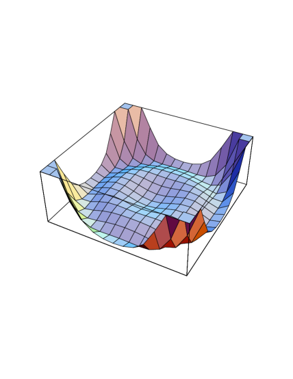
Figure 1. The potential energy as a function of $A$ at $B=f_{A}A-2f_{AA^{*}}AA^{*}$.

Are there any other minima of potential (5.23)? As can be seen from Figure 1, there is a second local minimum of $U_{0}$ given in (5.24) at which $U_{0}$ vanishes. It occurs for $|\left\langle A\right\rangle|^{2}=M_{P}^{2}$ or $\left\langle A\right\rangle=M_{P}e^{i\theta}$ for arbitrary real phase $\theta$. Note that this degeneracy in the vacuum is a direct consequence of the symmetry of the function $f$ in (5.21), and hence the Lagrangian, under the transformation $R\rightarrow e^{i\theta}R$. It follows from (5.25) that at this minimum $\left\langle f_{AA^{*}}^{-1}\right\rangle<0$ as required. Equation (5.19) then gives $\left\langle B\right\rangle=\frac{4}{3}M_{P}$. Therefore, the potential energy has a ring of local minima at

$$\begin{split}\left\langle A\right\rangle&=M_{P}e^{i\theta},\\ \left\langle B\right\rangle&=\tfrac{4}{3}M_{P},\end{split}$$ (5.30)

with vanishing cosmological constant. These are visible as the circular set of minima in Figure 1. To check that there are no ghosts in the theory around vacuum (5.30), we need to show that condition (5.18) is satisfied. We find that

$$\left\langle f+B+B^{*}\right\rangle=\tfrac{16}{9}>0$$ (5.31)

as required. Explicitly, expanding $A=\left\langle A\right\rangle+a$ and $B=\left\langle B\right\rangle+b$, it follows from (5.13) and (5.30) that to quadratic order

$$e^{-1}\mathcal{L}_{\text{KE-}AB}=-\tfrac{21}{8}\partial^{m}a\partial_{m}a^{*}-\partial^{m}c\partial_{m}c^{*},$$ (5.32)

where $c=\sqrt{3}(\frac{9b}{16}-e^{-i\theta}a)$, which is clearly non-ghostlike. The masses of the four real scalars are easily evaluated at this minimum, but the exact values are complicated and unenlightening. Suffice it to say that, in addition to the one zero-mass field in the direction of the circular set of minima, the three remaining masses are numerically different but of order $m$. Is supersymmetry broken at the vacua (5.30)? Using (5.29), we find that the Kähler covariant derivatives evaluated at (5.30) are

$$\begin{split}\left\langle D_{A}W\right\rangle&=32mM_{P},\\ \left\langle D_{B}W\right\rangle&=-\tfrac{15}{2}e^{i\theta}mM_{P}.\end{split}$$ (5.33)

It follows that supersymmetry is indeed spontaneously broken at these vacua (5.30). Substituting (5.22) into (2.23) gives the gravitino mass

$$m_{3/2}=\frac{27}{8}m,$$ (5.34)

which is of the same order as the non-vanishing scalar masses. Note that the supersymmetry breaking scale is set by $\left\langle D_{A}W\right\rangle$ and $\left\langle D_{B}W\right\rangle$, which are of order $mM_{P}$. It is conventional to denote this scale by $\mu=\sqrt{mM_{P}}$. The gravitino mass can then be written in the familiar form

$$m_{3/2}=\frac{27}{8}\frac{\mu^{2}}{M_{P}}.$$ (5.35)

With this definition, the non-vanishing scalar field masses at the non-trivial vacuum are of order $\mu^{2}/M_{P}$.

The preceding discussion is exact and valid at any energy scale. Indeed, as we have shown above, it is necessary to know the full theory in order to determine the vacuum structure. Once one has found the non-trivial supersymmetry breaking vacuum (5.30), however, it is of interest to consider small fluctuations around this vacuum, and to determine the effective theory for these fluctuations at energy scales much smaller than the Planck mass $M_{P}$. We now proceed to do this. Above we did not specify the value of the supersymmetry breaking scale $\mu$ relative to $M_{P}$. For the remainder of this discussion we will assume that $\mu\ll M_{P}$. For example, if we would like the gravitino mass to be of the order of the electroweak scale, that is $m_{3/2}\simeq 10^{2}\text{ GeV}$, then we must choose $\mu\simeq 10^{11}\text{ GeV}$, eight orders of magnitude smaller than $M_{P}$. Expanding around the non-trivial vacuum (5.30) with $\theta=0$, we define

$$\begin{split}\Phi&=M_{P}+\phi,\\ \Lambda&=\tfrac{4}{3}M_{P}+\lambda,\\ \end{split}$$ (5.36)

where $\phi$ and $\lambda$ are the fluctuations of $\Phi$ and $\Lambda$ around their vacuum expectation values, $M_{P}$ and $\tfrac{4}{3}M_{P}$ respectively. We will henceforth consider $\phi$ and $\lambda$ to be of the order of $\mu$ or smaller. The exact Lagrangian is given by expression (2.15) with Kähler potential and superpotential (5.22). At the scale $\mu$, since $\mu/M_{P}\ll 1$, the gravitational effects become negligible, and the supergravity Lagrangian (2.18) simplifies to the flat superspace Lagrangian given by

$$\mathcal{L}=\int d^{2}\theta d^{2}\bar{\theta}K+\left\{\int d^{2}\theta W+\text{h.c}\right\}.$$ (5.37)

However, in this regime we must also neglect terms in $K$ and $W$ suppressed by powers of $\mu/M_{P}$. That is the flat superspace Lagrangian (5.37) in fact reduces to

$$\mathcal{L}=\int d^{2}\theta d^{2}\bar{\theta}K^{\prime}+\left\{\int d^{2}\theta W^{\prime}+\text{h.c.}\right\},$$ (5.38)

where $K^{\prime}$ and $W^{\prime}$ are obtained by substituting (5.36) into (5.22) and keeping only the first non-trivial terms in $\mu/M_{P}$. Note that any terms in the Kähler potential which are constant or purely chiral plus antichiral, such as $\Phi^{\prime}+{\Phi^{\prime}}^{{\dagger}}$, do not contribute to Lagrangian (5.38). A constant term in the superpotential also does not contribute. In this limit, we find that

$$\begin{split}K^{\prime}&=\tfrac{45}{8}\phi\phi^{{\dagger}}-\tfrac{27}{16}(\phi\lambda^{{\dagger}}+\lambda\phi^{{\dagger}})+\tfrac{243}{256}\lambda\lambda^{{\dagger}},\\ W^{\prime}&=6\mu^{2}(\tfrac{4}{3}\phi+\lambda).\end{split}$$ (5.39)

We can diagonalize the Kähler potential by making the following field redefinitions

$$\begin{split}\Pi&=\sqrt{\tfrac{21}{8}}\phi,\\ \Sigma&=\sqrt{3}(\tfrac{9}{16}\lambda-\phi).\end{split}$$ (5.40)

In terms of superfields $\Pi$ and $\Sigma$, Kähler potential and superpotential (5.39) become

$$\begin{split}K^{\prime}&=\Pi\Pi^{{\dagger}}+\Sigma\Sigma^{{\dagger}},\\ W^{\prime}&=\tilde{\mu}^{2}\left(\sqrt{\tfrac{7}{2}}\Pi+\Sigma\right),\end{split}$$ (5.41)

where $\tilde{\mu}^{2}=\tfrac{32\sqrt{3}}{9}\mu^{2}$. The scalar field potential energy corresponding to (5.41) is simply a constant given by

$$V=\tfrac{9}{2}\tilde{\mu}^{4}.$$ (5.42)

Therefore, below the Planck scale, the theory behaves like a simple version of the O’Raifeartaigh model [16] with two chiral superfields, $\Pi$ and $\Sigma$. The positive definite value of the scalar potential signals supersymmetry breaking at scale $\mu$. Note that the Kähler potential and superpotential (5.41) look like a simple extension of the Polonyi model with two superfields. For comparison, let us consider the original Polonyi model for supersymmetry breaking [5]. The Polonyi model has one chiral superfield $Z$ with Kähler potential and superpotential given by

$$\begin{split}K&=ZZ^{{\dagger}},\\ W&=\mu^{2}(Z+\beta),\end{split}$$ (5.43)

where $\beta$ is a constant that is chosen to ensure vanishing cosmological constant. The exact theory is found to have a unique vacuum at

$$\left\langle Z\right\rangle=(\sqrt{3}-1)M_{P},$$ (5.44)

which has vanishing cosmological constant if $\beta$ is chosen to be $\beta=(2-\sqrt{3})M_{P}$. Supersymmetry is spontaneously broken with strength $\mu$ at this vacuum since

$$\left\langle D_{Z}W\right\rangle=\sqrt{3}\mu^{2}.$$ (5.45)

Expanding $Z=\left\langle Z\right\rangle+z$, and performing the same analysis as we did above, we find that the effective flat superspace Kähler potential and superpotential are given by

$$\begin{split}K^{\prime}&=zz^{{\dagger}},\\ W^{\prime}&=\mu^{2}z.\end{split}$$ (5.46)

The associated scalar field potential energy is

$$V=\mu^{4}.$$ (5.47)

Comparing (5.41) and (5.42) with (5.46) and (5.47) respectively, we see that our higher-derivative supergravitation model is, at low energy, simply a two superfield Polonyi model, with no essential differences. They only differ at the Planck scale. The Polonyi model can be thought of as the most trivial extension of the flat superspace O’Raifeartaigh model. In the Polonyi extension, one does not change the low energy superpotential or Kähler potential at the Planck scale, except for the addition of the constant term $\beta$ which is required to set the cosmological constant of the non-trivial vacuum to zero. However, this extension is by no means unique. As one goes up in energy, one could start seeing generic modifications to both the superpotential and the Kähler potential consisting of new terms that are suppressed by powers of the Planck mass. The theory constructed in this section is an explicit example of such a phenomenon.

We end this section by noting that there is a class of general higher-derivative supergravity theories which have a no-scale structure, with flat directions in the scalar potential. In the previous section, when $f(R,R^{{\dagger}})$ could be decomposed into $f(R)+f(R^{{\dagger}})$, we found that choosing $F(R)=Rf(R)=cR^{-3/2}$ made the scalar potential identically zero. In fact, the transformed theory, in terms of the new chiral field $\Phi$, was identical to pure no-scale supergravity. In the general case, we see that we cannot chose $f(R,R^{{\dagger}})$ such that the whole scalar potential is zero because the second, quadratic, term in $U$ (5.16) cannot be made to vanish. However, choosing $f(R,R^{{\dagger}})$ can introduce flat directions into the potential, giving a continuous set of degenerate vacua with zero cosmological constant. The maximum possible degeneracy is acheived by setting the first term in the potential, $U_{0}$ (5.20), to zero. The general form of $f(R,R^{{\dagger}})$ with this property is

$$f\left(R,R^{{\dagger}}\right)=\sqrt{RR^{{\dagger}}}\left[h(R)+\left(h(R)\right)^{{\dagger}}\right],$$ (5.48)

where $h(R)$ is an arbitrary complex function of $R$. The Kähler potential and superpotential for the transformed theory are then given by

$$K =-3\ln\left\{\sqrt{\Phi\Phi^{{\dagger}}}\left[h(\Phi)+\left(h(\Phi)\right)^{{\dagger}}\right]+\Lambda+\Lambda^{{\dagger}}\right],$$ (5.49)

$$W =6\Phi\Lambda.$$

and the scalar potential becomes

$$V=-\frac{48|A|}{\left[|A|(h+h^{*})+B+B^{*}\right]^{2}\left[h+Ah^{\prime}+h^{*}+A^{*}{h^{\prime}}^{*}\right]}\left|B+\left|A\right|A^{*}{h^{\prime}}^{*}\right|^{2},$$ (5.50)

where $h^{\prime}=dh/dA$. Considered as a function of $B$, the potential is clearly only bounded from below if the prefactor in (5.50) is positive. As before this gives the condition that at the vacuum

$$\left\langle f_{AA^{*}}^{-1}\right\rangle=\left\langle|A|\left(h+Ah^{\prime}+h^{*}+A^{*}{h^{\prime}}^{*}\right)\right\rangle<0.$$ (5.51)

As before to ensure that the $A$ and $B$ fields have non-ghost-like propagation we require $\left\langle f+B+B^{*}\right\rangle>0$. It is clear that setting $B=-|A|A^{*}{h^{\prime}}^{*}$ sets the potential to zero, independent of the value of $A$. Thus the potential has flat directions, with a continuous set of vacua, stable provided (5.51) is satisfied, and given by

$$\left\langle A\right\rangle =A_{0},$$ (5.52)

$$\left\langle B\right\rangle =-\left|A_{0}\right|A_{0}^{*}\left[h^{\prime}(A_{0})\right]^{*}.$$

As in the pure no-scale model, all these vacua break supersymmetry, with zero cosmological constant. The value of the gravitino mass depends on the vaccum in question and is given by

$$m_{3/2}=\frac{\left|\left\langle A\right\rangle\right|^{3}\left|\left\langle h^{\prime}\right\rangle\right|^{2}}{\left\langle h-Ah^{\prime}+h^{*}-A^{*}{h^{\prime}}^{*}\right\rangle}.$$ (5.53)

The important point here, as in all no-scale models, is that the flat directions in the scalar potential imply that the vacuum is undetermined. As a result the value of the gravitino mass is also undetermined at tree level.

6. Conclusion

We have shown in this paper that higher-derivative $N=1$ supergravity in four dimensions has non-trivial vacua with vanishing cosmological constant that spontaneously break supersymmetry. This result opens the possibility of a new approach to supersymmetry breaking in phenomenological supergravity theories and, perhaps, in superstring theories. In this new approach, supersymmetry is spontaneously broken by a non-trivial vacuum of the new degrees of freedom associated with higher-derivative supergravitation, and does not need a hidden sector or gaugino condensates. A more complete understanding of this approach to supersymmetry breaking requires coupling higher-derivative supergravity to matter and examining the effect of the non-trivial supergravity vacuum on the low energy matter Lagrangian. It is clear that supersymmetry will be broken in this Lagrangian, but the details of the pattern and strength of this breaking require careful study. This study is presently underway [17].

References

- [1] A. Hindawi, B. A. Ovrut, and D. Waldram, Consistent spin-two coupling and quadratic gravitation, Phys. Rev. D 53 (1996), 5583–5596, hep-th/9509142.
- [2] A. Hindawi, B. A. Ovrut, and D. Waldram, Non-trivial vacua in higher- derivative gravitation, Phys. Rev. D 53 (1996), 5597–5608, hep-th/9509147.
- [3] A. Hindawi, B. A. Ovrut, and D. Waldram, Two-dimensional higher-derivative supergravity and a new mechanism for supersymmetry breaking, Nucl. Phys. B471 (1996), 409–429, hep-th/9509174.
- [4] E. Cremmer, S. Ferrara, C. Kounnas, and D. V. Nanopoulos, Naturally vanishing cosmological constant in supergravity, Phys. Lett. 133B (1983), 61–66.
- [5] J. Poloyni, Budapest Preprint KFKI-93 (1977).
- [6] K. Foerger, B. A. Ovrut, S. Theisen, and D. Waldram, Higher derivative gravity in string theory, Phys. Lett. 388B (1996) 512–520, hep-th/9605145.
- [7] J. Wess and J. Bagger, Supersymmetry and supergravity, 2nd ed., Princeton University Press, Princeton, 1992.
- [8] E. Cremmer, B. Julia, J. Scherk, S. Ferrara, L. Girardello, and P. van Nieuwenhuizen, Spontaneous symmetry breaking and Higgs effect in supergravity without cosmological constant, Nucl. Phys. B147 (1979), 105–131.
- [9] G. Magnano, M. Ferraris, and M. Francaviglia, Nonlinear gravitational Lagrangians, Gen. Rel. Grav. 19 (1987), 465–479.
- [10] A. Jakubiec and J. Kijowski, On theories of gravitation with nonlinear Lagrangians, Phys. Rev. D 37 (1988), 1406–1409.
- [11] M. Ferraris, M. Francaviglia, and G. Magnano, Do nonlinear metric theories of gravitation really exist?, Class. Quantum Grav. 5 (1988), L95–L99.
- [12] G. Magnano, M. Ferraris, and M. Francaviglia, Legendre transformation and dynamical structure of higher-derivative gravity, Class. Quantum Grav. 7 (1990), 557–570.
- [13] S. Ferrara, M. T. Grisaru, and P. van Nieuwenhuizen, Poincaré and conformal supergravity models with closed algebras, Nucl. Phys. B138 (1978), 430–444.
- [14] S. Cecotti, Higher derivative supergravity is equivalent to standard supergravity coupled to matter, Phys. Lett. 190B (1987), 86–92.
- [15] B. A. Ovrut and S. Kalyana Rama, Lorentz and Chern-Simons terms in new minimal supergravity, Phys. Lett. 254B (1991), 132–138.
- [16] L. O’Raifeartaigh, Spontaneous symmetry breaking for chiral scalar superfields, Nucl. Phys. B96 (1975), 331.
- [17] A. Hindawi, B. A. Ovrut, and D. Waldram, Soft supersymmetry breaking induced by higher-derivative supergravitation in the electroweak standard model, Phys. Lett. 381B (1996), 154–162, hep-th/9602075.