hep-th/9511211

THU-95/33

November 1995

Some approaches to 2+1-dimensional gravity
coupled to point-particles
M.Welling

Instituut voor Theoretische Fysica
Rijksuniversiteit Utrecht
Princetonplein 5
P.O. Box 80006
3508 TA Utrecht
The Netherlands

Introduction

In 1963 Staruszkiewicz considered for the first time gravity in 2+1 dimensions coupled to point-particles [2]. In 1984 the subject was reconsidered by Gott, Alpert, Giddings, Abbot, Kuchar, Deser, Jackiw and ’t Hooft [3]. In these articles they found solutions for the gravitational field around N static point-particles. They also solved the case of one spinning particle located at the origin. The key result was that locally these space-times are flat except at the particles positions. This implies that the gravitational field contains no degrees of freedom as can also be deduced from a simple counting argument: We have 6 independent metric components minus 3 first-class constraints minus 3 gauge-fixing conditions, resulting in 0 degrees of freedom. The reason that these spaces are not completely trivial is because of non-trivial boundary conditions on the (flat) coordinates. For instance, in the case of a massive point-particle sitting at the rest in the origin, we have to cut a wedge out of space-time and identify opposite points of the wedge. So the range of the angular coordinate $\varphi$ is: $\varphi\in[0,2\pi(1-4mG)]$ (m is the mass of the particle). In general this identification condition on the coordinates is not a simple rotation but a Poincaré-transformation (see section 1). Not much later Deser and Jackiw found solutions for gravity with a cosmological constant. The case $\Lambda>0$ (de Sitter space) coupled to 2 static, antipodal particles was solved [4]. In a geometrical approach ’t Hooft solved the N-particle case ($\Lambda=0$), and proved that a Cauchy-formulation was possible within which no closed timelike curves could occur [5]. A different view on the problem was provided by Achucarro and Townsend and later by Witten [6]. They considered a Chern-Simons theory with a gauge-field $A_{\mu}$ taking values in the Poincaré-algebra, and proved that this theory is equivalent to 2+1 dimensional gravity. Later Grignani and Nardelli invented a consistent way to couple point-particles to this gauge field [7]. This Chern-Simons approach is closely related to the description of gravity using Ashtekar variables [27]. It is however not known to me if people considered the coupling of point-particles (For a review on loop-quantisation one should consult the lecture by Kirill Krasnov in this volume). Finally I would like to mention Waelbroeck’s approach [14] who consideres these Ashtekar variables on a lattice in order to obtain a finite set of degrees of freedom. This is an exact description because only the handles and particles are the true degrees of freedom.

A first step towards quantisation was made by Mazur, ’t Hooft, Deser, Jackiw and de Sousa Gerbert who studied the scattering of 2 quantum particles. [9]. Later the calculation was also done in the Chern-Simons approach [10]. Carlip considered the scattering of N particles where he stressed the role of the braid-group in 2+1-gravity [10]. All these approaches have their own way of quantising the theory. The problem is however that not all these quantisations seem to be equivalent as shown by Carlip [8]. In a way this is disappointing, but it reflects the fact that the problems encountered in quantising 3+1-dimensional gravity still survive the dimensional reduction to 2+1 dimensions. As the theory contains no gravitons, and therefore has a finite set of degrees of freedom, some of the problems must be connected with the covariance of the theory under coordinate transformations. The hope is of course that we are able to solve these problems in the much simpler model of 2+1-gravity. The big challenge will be to formulate a consistent second quantised theory of 2+1 -gravity and look into the problems of renormalisation. This issue has not been adressed to my knowledge up to now. Finally I would like to mention that there is a close relationship of 2+1-gravity with the theory of topological defects in condensed matter physics [16].

In this review that is based on a lecture given at the Kazan Summer School 1995, we discuss 2+1-gravity coupled to point particles. In section 1 we shortly look at the solutions found in [3] and [4]. In section 2 we give the essential ingredients of the polygon-approach of ’t Hooft. In section 3 a short introduction is given to the Chern-Simons formulation of 2+1-gravity. Finally we will discuss reference [12] where a new gauge is introduced which is very convenient for the description of particles. Almost nowhere I will go into the issues of quantisation deeply, but will restrict myself to general remarks. On the different ways to quantise the theory excellent reviews exist[13]. I am well aware that this survey is only a poor selection out of a vast amount of papers that have appeared on the subject. I only restrict myself to the issues adressed at the summer school with the exception of the second part of section 1 where gravity with a cosmological constant is treated.

1 The Geometrical Appraoch

In this section we will give some simple exact solutions of the gravitational field surrounding point-particles. Both the case $\Lambda=0$ and $\Lambda\neq 0$ will be treated.

In 2+1 dimensions the Einstein equations with a cosmological constant are given by the same expression as in 3+1 dimensions:

$$G^{\mu\nu}-\Lambda g^{\mu\nu}=8\pi GT^{\mu\nu}$$ (1)

A special feature of 2+1 dimensions is however that we can express the curvature-tensor in the following way:

$$R^{\mu\nu}_{~{}~{}~{}\alpha\beta}=\varepsilon^{\mu\nu\lambda}\varepsilon_{\alpha\beta\sigma}G^{\sigma}_{\lambda}$$ (2)

Using (1) this can be written as:

$$R^{\mu\nu}_{~{}~{}~{}\alpha\beta}=8\pi G\varepsilon^{\mu\nu\lambda}\varepsilon_{\alpha\beta\sigma}T^{\sigma}_{\lambda}+\Lambda(\delta^{\mu}_{\alpha}\delta^{\nu}_{\beta}-\delta^{\nu}_{\alpha}\delta^{\mu}_{\beta})$$ (3)

This implies that outside sources the curvature must be constant.

$$R\equiv R^{\mu\nu}_{~{}~{}~{}\mu\nu}=6\Lambda$$ (4)

From this we deduce that the gravitational field has no local degrees of freedom (there are no gravitational waves). Setting $\Lambda=0$ for the moment and considering a pointlike particle at the origin we have:

$$T^{00}=m\delta^{2}(\vec{r})~{}~{}~{}~{}~{}~{}~{}~{}T^{0i}=0~{}~{}~{}~{}~{}~{}~{}~{}T^{ij}=0~{}~{}~{}~{}~{}~{}~{}i,j=1,2$$ (5)

By symmetry arguments we have $g_{0i}=0$. The nontrivial Einstein equations are given by:

$$G^{0}_{0} = -\frac{1}{2}{{}^{(2)}R}=8\pi Gm\delta^{2}(\vec{r})$$ (6)

$$G_{ij} = -\frac{1}{2N}(D_{i}D_{j}-\gamma_{ij}D^{2})N=0$$ (7)

Here $\gamma_{ij}$ is the intrinsic 2 dimensional metric and $D_{i}$ is the covariant derivative defined with respect to that metric, ${}^{(2)}R$ is the 2 dimensional curvature scalar. Futhermore N is the well known lapse function which equals in this static case $g_{00}=-N^{2}$. Taking the trace of equation (7) we notice that we have to solve

$$D^{2}N=0~{}~{}~{}~{}D_{i}D_{j}N=0$$ (8)

which is solved by $N=$constant. We redefine $t$ so that $N=1$. In 2 dimensions we can always choose coordinates so that $\gamma_{ij}=e^{\phi}\delta_{ij}$. Using this in equation (6) we find:

$$\vec{\nabla}^{2}\phi=-16\pi Gm\delta^{2}(\vec{r})$$ (9)

This is easily solved using $\vec{\nabla}^{2}\ln r=2\pi\delta^{2}(\vec{r})$:

$$e^{\phi}=Cr^{-8Gm}$$ (10)

Absorbing the constant C into r we finally have:

$$ds^{2}=-dt^{2}+r^{-8Gm}(dr^{2}+r^{2}d\varphi^{2})$$ (11)

Because we know that the curvature vanishes everywhere except at the particles positions we can transform to local flat coordinates:

$$\rho = \frac{r^{\beta}}{\beta}~{}~{}~{}~{}~{}~{}\beta=1-4Gm$$ (12)

$$\theta = \beta\varphi$$ (13)

$$ds^{2} = -dt^{2}+d\rho^{2}+\rho^{2}d\theta^{2}$$ (14)

Although the situation looks trivial now we have to be carefull. The new coordinate $\theta$ ranges from 0 to $2\pi\beta$. So there is a deficit angle in space (see figure 1)

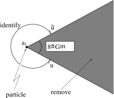
Figure 1: The wedge cut out of space-time

The most important lesson we have to draw from this is that it is always possible to transform to coordinates in which $g_{\mu\nu}=\eta_{\mu\nu}$, but that there is a price to be paid. The price is that we have multivalued coordinates (or coordinates with strange boundary conditions). This solution is easily generalized to N static particles. In this case it proves more convenient to go to complex coordinates:

$$z=x+iy~{}~{}~{}~{}~{}~{}\bar{z}=x-iy$$ (15)

In these coordinates the line element for N static particles becomes:

$$ds^{2}=-dt^{2}+\prod_{i=1}^{N}(z-a_{i})(\bar{z}-\bar{a}_{i})^{-4Gm_{i}}dzd\bar{z}$$ (16)

This is a multiconical space. Transforming to flat coordinates by using the transformation:

$$u=\int^{z}dz^{\prime}\prod_{i=1}^{N}(z^{\prime}-a_{i})^{-4Gm_{i}}~{}~{}~{}~{}~{}~{}\bar{u}=c.c.$$ (17)

we construct a space from which we have to remove wedges emanating from every particle. In this static case it is still unimportant in which direction we choose the wedge. If however the particle moves, it is handy to choose the wedge behind the particle or in front of the particle. We will now argue why. In the static case the wedge is characterised by an identification rule:

$$\tilde{u}^{a} = R^{a}_{~{}b}u^{b}$$ (18)

$$R^{a}_{~{}b} = \left(\begin{array}[]{ccc}1&0&0\\ 0&\cos 2\pi\alpha&\sin 2\pi\alpha\\ 0&-\sin 2\pi\alpha&\cos 2\pi\alpha\\ \end{array}\right)~{}~{}~{}~{}~{}~{}~{}\alpha=4Gm$$ (22)

Here $\tilde{u}^{a}$ is a point on one side of the wedge and $u^{a}$ the point on the opposite side of the wedge. If the particle moves, the identification-rule is still the same in its restframe. In the moving frame we therefore have:

$$\tilde{u}^{a}=(BRB^{-1})^{a}_{~{}b}u^{b}$$ (23)

Here $B^{a}_{~{}b}$ is a boost matrix with arbitrary rapidity $(\eta)$ and in an arbitrary direction. In order to avoid a time jump we have to choose the wedge symmetrically behind or before the particle. The effect is then that the wedge becomes a bit larger. This is to be expected as the energy of the moving particle is also larger.

The particle could also carry spin (classically). The energy momentum tensor then looks like:

$$T^{00}=m\delta^{2}(\vec{r})~{}~{}~{}~{}~{}~{}~{}T^{0i}=\frac{1}{2}S\varepsilon^{ij}\partial_{j}\delta^{2}(\vec{r})~{}~{}~{}~{}~{}~{}~{}T^{ij}=0$$ (24)

Solving the Einstein equations is considerably more difficult ($g_{0i}\neq 0$) and we will not repeat the derivation here. It can be found in [3]. Instead we will immediately give the result:

$$ds^{2}=-(dt^{2}+2Adtd\varphi+A^{2}d\varphi^{2})+(dr^{2}+r^{2}d\varphi^{2})$$ (25)

Where $A=4GS$ is the spin of the particle. The important issue is again that we can transform to the Minkowski line-element by the transformation:

$$T=t+A\varphi$$ (26)

This has the strange consequence that we need a cut in space over which time jumps by an amount $8\pi GS$. This also implies that close to the particle, closed time-like curves are possible. Generalisations to N massive, spinning particles exist [15] but we will not treat that futher here. The lesson is clear: Space-times with N moving, massive and spinning particles can be constructed by cutting out wedges in space and define identifications over the these wedges. Generaly, these identifications are an element of the Poincaré group. As an example we treat the 2 particle case, with total angular momentum J.

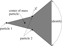
Figure 2: Wedge cut out around 2 particles.

We can always choose the particles on the x-axis. If we cut out the wedges as in figure 2 we have the following identification:

$$\tilde{u}=a_{1}+B_{1}R_{1}B_{1}^{-1}(a_{2}-a_{1}+B_{2}R_{2}B_{2}^{-1}(u-a_{2}))$$ (27)

where we didn’t show the indices, and $a_{i}$ is the position of particle $i$. Note that we didn’t choose the wedge of the second particle at its tail, introducing a time jump over the (total) wedge. The transformation is precisely a Poincaré transformation:

$$\tilde{u} = \Lambda u+q$$ (28)

$$\Lambda = B_{1}R_{1}B_{1}^{-1}B_{2}R_{2}B_{2}^{-1}$$ (29)

$$q = B_{1}R_{1}B_{1}^{-1}(a_{2}-a_{1})+a_{1}-B_{1}R_{1}B_{1}^{-1}B_{2}R_{2}B_{2}^{-1}a_{2}$$ (30)

If we write:

$$\Lambda=B_{\bf com}R_{\bf com}B_{\bf com}^{-1}$$ (31)

this transformation really desribes a center of mass particle that is boosted to a speed $v=\tanh\eta$. We still have the freedom to choose the overall Lorentzframe so that we may take:

$$\Lambda=R_{\bf com}$$ (32)

Futhermore we may place the c.o.m.-particle at the origin by demanding $q^{i}=0$. Comparison with a spinning particle at rest in the origin suggests that the total angular momentum is given by the time component of the translation vector $q^{a}$:

$$J=[B_{\bf com}^{-1}q]^{0}=-[B_{1}R_{1}B_{1}^{-1}(a_{2}-a_{1})]^{0}=-[B_{2}R_{2}B_{2}^{-1}(a_{2}-a_{1})]^{0}$$ (33)

In the limit $G\rightarrow 0$ we can indeed recover the special relativistic result. In the next section we will also treat multiparticle solutions, but then we will consequently put the wedges behind the particles in order to make a Cauchy formulation possible (no time jumps). The total angular momentum expresses itself then as a space-like translation over the total wedge.

Next we consider space-times with $\Lambda\neq 0$. The relevant reference is [4]. Again we consider static configurations ($g_{0i}=0$) and choose conformal coordinates on a time=constant slice: $\gamma_{ij}=e^{\phi}\delta_{ij}$. The Einstein equations for a static configuration of particles (without spin) is:

$$\partial\bar{\partial}\phi+\frac{\Lambda}{2}e^{\phi}=-4\pi GN^{2}\sum^{N}_{i=1}m_{i}\delta^{2}(z-a_{i})$$ (34)

$$\partial\bar{\partial}N+\frac{\Lambda}{2}e^{\phi}N=0$$ (35)

$$\bar{\partial}V=\partial\bar{V}=0$$ (36)

$$V=\frac{1}{\Lambda}e^{-\phi}\partial N~{}~{}~{}~{}~{}~{}~{}~{}~{}~{}\bar{V}=\frac{1}{\Lambda}e^{-\phi}\bar{\partial}N$$ (37)

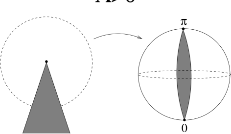
Figure 3: de Sitter space-time with a particle at the origin

Here we used the notation: $\partial=\frac{\partial}{\partial z}$ and $\bar{\partial}=\frac{\partial}{\partial\bar{z}}$. An additional condition is that initial static particles only remain static if $\Gamma^{i}_{00}$ vanishes at the location of the source. One can show that this implies: $NV=N\bar{V}=0$ at the source. Of course we must also insist that $N$ and $e^{\phi}$ are real and single-valued functions. Taking into account the above considerations we can write down the following solutions for $\Lambda>0$:

$$e^{\phi}=\frac{4\partial f\bar{\partial}\bar{f}}{\Lambda(1+f\bar{f})^{2}}$$ (38)

$$N=\frac{1-f\bar{f}}{1+f\bar{f}}$$ (39)

where $f=f(z)$ is a holomorphic function and $\bar{f}=\bar{f}(\bar{z})$ is an anti-holomorphic function. Also for $\Lambda<0$ we can check that we have the solutions:

$$e^{\phi}=\frac{4\partial f\bar{\partial}\bar{f}}{|\Lambda|(1-f\bar{f})^{2}}$$ (40)

$$N=\frac{1+f\bar{f}}{1-f\bar{f}}$$ (41)

In order to reproduce delta-functions in equation (34) we demand that at $z=a_{i}$ we have the following singular behaviour for $\phi$:

$$\phi\sim-4Gm_{i}N^{2}(a_{i})\ln(z\bar{z})+\mbox{regular terms}$$ (42)

The case of 1 particle sitting in the origin is now easily solved by:

$$f=z^{-\beta}~{}~{}~{}~{}\bar{f}=\bar{z}^{-\beta}~{}~{}~{}~{}~{}\beta=1-4Gm$$ (43)

We can check that $N$ is regular at the origin so that we can actually scale it to 1 at $r=0$. We see that in both cases the metric becomes pathological near $r=1$. In the case $\Lambda<0$ this means that physical infinity is situated at coordinate distance $r=1$. However in the case $\Lambda>0$ this is just an artifact of the coordinate system and we may change to coordinates that cover the whole sphere. In order to visualise these solutions it is convenient to use the following embedding:

$$Z = \frac{1-f\bar{f}}{1+f\bar{f}}~{}~{}~{}~{}~{}~{}~{}~{}~{}~{}~{}\Lambda>0$$ (44)

$$U = \frac{2f}{1+f\bar{f}}~{}~{}~{}~{}~{}~{}~{}~{}~{}~{}~{}~{}\bar{U}=c.c.$$ (45)

$$T = \frac{1+f\bar{f}}{1-f\bar{f}}~{}~{}~{}~{}~{}~{}~{}~{}~{}~{}\Lambda<0$$ (46)

$$U = \frac{2f}{1-f\bar{f}}~{}~{}~{}~{}~{}~{}~{}~{}~{}~{}~{}~{}\bar{U}=c.c.$$ (47)

In the case $\Lambda>0$ this is just the stereographic projection, in the case $\Lambda<0$ this is a projection from a hyperboloid to the plane. In the $f$-plane the solution is pictured by cutting out a wedge emanating from the particle’s location $f=0$ (as in section 1 the angle variable of $f$ ranges from 0 to $2\pi(1-4Gm)$). Mapping this on the sphere and the hyperboloid using the above embedding results in the above pictures (figures 3,4).

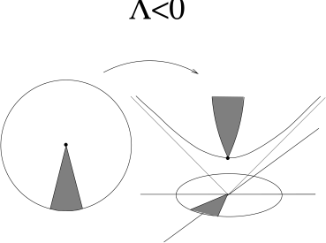
Figure 4: Anti de Sitter space-time with a particle at the origin

In the case $\Lambda>0$ we see that the solution realy represents 2 antipodal particles. In the second case we have found the Poincaré-disk (Lobachevsky-space) from which a wedge is removed between 2 geodesics. It is important to notice that in both cases a loop traversed around a particle would result in a transformation:

$$f\rightarrow e^{2\pi i\beta}f$$ (48)

$$\bar{f}\rightarrow e^{-2\pi i\beta}\bar{f}$$ (49)

One can check that the expressions for $e^{\phi}$ and $N$ are invariant under these transformations (as they should be by the requirement of single-valuedness). In the case of de Sitter space one expects that static configurations of more than 2 particles do exist. It is however not known to us if there exist explicit solutions in the literature.

2 The Polygon Approach

The relevant references are [5]. The fact that the gravitational field has no degrees of freedom calls for an approach in which only a finite set of degrees of freedom survive (the only degrees of freedom of the theory are in fact the positions and momenta of the particles). This is precisely what happens in what we call the Polygon approach to 2+1-gravity coupled to point-particles. It was invented by ’t Hooft to prove that no closed time-like curves can occur in a closed universe. He proved that the universe would crunch before the CTC could be finished. The basic idea behind this method is to divide space up into rectilinear polygons with vertices where 3 seams meet (see figure 5)

Figure 5: Space divided up in polygons.

Figure 6: Polygons in the x-t axis

Just like in Regge-calculus, inside each polygon the space is flat and the metric is simply Minkowskian. When we move over a seam and enter a new polygon the coordinates we will change according to a Lorentz-transformation. Thus on every polygon we choose different Lorentzframes. Futhermore we demand the following 3 conditions:

• On every polygon there is a rest frame such that it is an equal time surface.

• At any time the total surface is a Cauchy surface and it is chosen to be equal time everywhere.

• The metric must be continuous at the seams.

Also particles are incorporated in this model. They sit at the end of a 1-vertex (see figure 5). Using the above rules and our knowledge of 1 particle solutions we can deduce the following rules:

1. The lengths of the seams are equal as considered from 2 adjacent polygons.

2. The speed of the seams is always orthogonal to the seam and equal in magnitude as considered from the 2 adjacent rest frames (see figure 7).

   

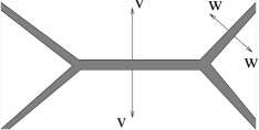
   Figure 7: Moving seams

3. The deficit angle is always in front or behind a particle (in order to avoid time jumps; see figure 8).

   

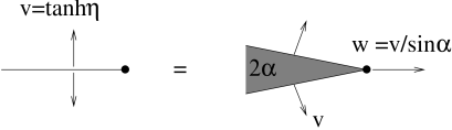
   Figure 8: Wedge behind the particle

4. At the 3-vertices (where no mass is present), there are relations between the boost parameters $\eta_{i}$ and angles $\alpha_{i}$ (see figure 9).

   

   Figure 9: 3-Vertex

   These can be deduced from the fact that the 3 dimensional curvature must vanish at the vertex (although the 2 dimensional curvature may be different from zero). Roughly speaking; 3 quantities determine 3 other quantities. One has to take care however of inequalities such as the triangle inequality: $|\eta_{1}|+|\eta_{2}|\geq|\eta_{3}|$.

5. As the system starts to evolve all kinds of transitions will take place (actually 9 different kinds). We will only picture 2 examples in figure 10.

   

   Figure 10: 2 Possible transitions

   The transition from one situation to the next is a completely determininistic proces, i.e. all the new variables ($\eta_{i},\alpha_{i},L_{i}$) can be calculated from the old ones. In this way we have a completely deterministic model, free of pathologies with a finite set of degrees of freedom that can be used to study 2+1 dimensional gravity.

It is also possible to write down a Hamiltonian formulation for this model. As the total energy in 2+1 gravity is equal to the total deficit angle it is a logical step to take the total sum of all deficits as the Hamiltonian of the theory. Firstly we have a deficit angle of $H_{P}=2\alpha_{P}$ for a particle. Secondly there is a possible deficit at a 3-vertex of $H_{V}=2\pi-\alpha_{V}^{1}-\alpha_{V}^{2}-\alpha_{V}^{3}$ see figure 9). The total Hamiltonian is now given by:

$$H_{\bf tot}=\sum_{i}H_{P_{i}}+\sum_{j}H_{V_{j}}\\$$ (50)

As configuration variables we use the lengths of the seams: $L_{i}(\geq 0)$. We already mentioned that is was possible to express the angles $\alpha_{V_{j}}^{l}$ in terms of 3 neighbouring boostparameters $\eta_{i}$. Also the $\alpha_{P_{i}}$ can be expressed in terms of the mass $m_{i}$ and boostparameter $\eta_{i}$ at his tail. Moreover it is known how fast the lengths $L_{i}$ grow, i.e. $\frac{d}{dt}L_{i}$ can also be expressed in terms of neighbouring $\eta_{i}$ (it is constant in time). We can use this information together with the equation of motion:

$$\frac{d}{dt}L_{i}=\{H_{\bf tot},L_{i}\}$$ (51)

to derive that

$$p_{i}=2\eta_{i}$$ (52)

The $L_{i},2\eta_{j}$ are canonically conjugate phase space variables:

$$\{L_{i},2\eta_{j}\}=\delta_{ij}$$ (53)

The other equation of motion is trivial because the Hamiltonian $H(\alpha_{i}(\eta_{j}))$ only depends on the momenta:

$$\frac{d}{dt}p_{i}=\{H_{\bf tot},p_{i}\}=0$$ (54)

The simplicity is however a bit deceiving because we have to incorporate some constraints in the model. The constraints could be expected since the number of canonical variables exceeds the number of true degrees of freedom, which are only connected with particles. One can very easily understand these constraints. First of all the angles inside the polygon must add up to $(m-2)\pi$ where m is the number of angles.

$$C_{1}=\sum_{i=1}^{m}\alpha_{i}-(m-2)\pi=0$$ (55)

Secondly, the variables $L_{i}$, written as vectors, must add up to zero:

$$\vec{C}_{2}=\sum_{i=1}^{m}\vec{L_{i}}=0$$ (56)

This can be reformulated in complex notation as:

$$C_{2}=\sum_{k=1}^{m}L_{k}e^{i\theta_{k}}=0~{}~{}~{}~{}~{}~{}~{}~{}~{}~{}~{}\theta_{k}=\sum_{j=1}^{k-1}(\pi-\alpha_{j})$$ (57)

Futhermore we like to remind the reader that there are still the following inequalities:

$$L_{i}\geq 0$$ (58)

$$|\eta_{i}|+|\eta_{j}|\geq|\eta_{k}|~{}~{}~{}~{}\mbox{and cyclic permutations}$$ (59)

which are hard to handle. The constraints (55,57) are first class and generate gauge transformations in the model. The first constraint evolves one polygon in time. As a result the surrounding seams change their position. The second constaint changes to a different Lorentz-frame inside the polygon. Obviously, again all seams start to change. It can be calculated that these changes are properly given by:

$$\delta L_{i}=\{L_{i},C_{j}\}~{}~{}~{}~{}~{}~{}~{}~{}~{}\delta p_{i}=\{p_{i},C_{j}\}~{}~{}~{}j=1,2$$ (60)

One can also check that the constraint algebra closes properly. This is not a trivial task at all and the algebra is highly nonlinear. With that we mean that it is not of the simple form $\{C_{i},C_{j}\}=A^{k}_{ij}C_{k}$, but on the righthand side for instance a $\sin(C_{i})$ can appear. Of course the nontrivial part of the evolution are the transitions that can take place and they have to be dealt with separately. Now that we have formulated a Hamiltonian theory, the way to quantisation seems to be open. One simply changes Poisson-Brackets by commutators:

$$\{.,.\}\rightarrow-i\hbar[.,.]$$ (61)

Next one chooses for instance to work in the $L_{i}$ representation and writes down a wave function:

$$\Psi_{D}(L_{1},...,L_{N})$$ (62)

where D denotes its dependence on the diagram. First of all one needs to take into account the transitions. They must be incorporated as boundary conditions on the wave function. Needless to say that for a complicated diagram this is a very difficult task. Also the constraints and inequalities should be taken into account as constraints on the wavefunction to select the physical Hilbertspace. Although some improvement can be gained by choosing clever coordinates it still remains a very difficult task to complete this quantisation scheme. This will be one of the motivations in section 4 to go to a single-valued coordinate system. One can already deduce one important result in the quantum heory. As we can only write down expressions for $\sin H$ and $\cos H$ we only have an expression for the evolution-operator $e^{-iHt}$ and not for $H$ itself. This implies that we cannot distinguish between $e^{-iHt}$ and $e^{-i(H+2\pi n)t}$. In order to avoid multi-valuedness we have to conclude that t is integer-valued. So the model has discretised time!

3 Gauge Theory of Gravity

In this section we will briefly review some of the aspects of of the Chern-Simons approach to gravity and the way it is coupled to point-particles. The references are here ([7]). The main result is that the Einstein-Hilbert action is equivalent to a Chern-Simons action where the gauge field $A_{\mu}$ takes values in the Poincaré algebra ISO(2,1). If we write $J^{a}=\frac{1}{2}\varepsilon^{abc}J_{bc}$ for the SO(2,1) generators and $P^{a}$ for the generators of translations, the algebra is:

$$[J^{a},J^{b}]=\varepsilon^{abc}J_{c}~{}~{}~{}~{}[J^{a},P^{b}]=\varepsilon^{abc}P_{c}~{}~{}~{}~{}~{}[P^{a},P^{b}]=0$$ (63)

The gauge fields are then decomposed into:

$$A_{\mu}=e^{~{}~{}a}_{\mu}P_{a}+\omega_{\mu}^{~{}~{}a}J_{a}$$ (64)

Here $e^{~{}~{}a}_{\mu}$ (the dreibein or tetrad) is considered as the gauge field for translations and $\omega^{~{}~{}a}_{\mu}=\frac{1}{2}\varepsilon^{abc}\omega_{\mu bc}$ (the spin connection) as the gaugefield for Lorentztransformations. The usual Chern-Simons action is:

$$I_{CS}=\int d^{3}x~{}\varepsilon^{\mu\nu\rho}{\bf Tr}(A_{\mu}\partial_{\nu}A_{\rho}+\frac{2}{3}A_{\mu}A_{\nu}A_{\rho})$$ (65)

is invariant under the following gauge transformations:

$$\delta A_{\mu} = -{\cal D}_{\mu}\Lambda(x)$$ (66)

$$= -\partial_{\mu}\Lambda-[A_{\mu},\Lambda]$$ (67)

The gauge parameter $\Lambda$ can also be decomposed in terms of independent gauge parameters for Lorentztransformations and translations:

$$\Lambda=\rho^{a}(x)P_{a}+\kappa^{a}(x)J_{a}$$ (68)

The gauge transformations for the dreibein and the spinconnection are also decomposed into local Lorentztransformations:

$$\delta_{1}e^{~{}~{}a}_{\mu} = \varepsilon^{a}_{~{}~{}bc}e^{~{}~{}b}_{\mu}\kappa^{c}$$ (69)

$$\delta_{1}\omega^{~{}~{}a}_{\mu} = \partial_{\mu}\kappa^{a}+\varepsilon^{a}_{~{}~{}bc}\omega_{\mu}^{~{}~{}b}\kappa^{c}$$ (70)

and local translations:

$$\delta_{2}e^{~{}~{}a}_{\mu} = \partial_{\mu}\rho^{a}+\varepsilon^{a}_{~{}~{}bc}\omega^{~{}~{}b}_{\mu}\rho^{c}$$ (71)

$$\delta_{2}\omega^{~{}~{}a}_{\mu} = 0$$ (72)

Witten has shown [6] that these gauge transformations are equivalent (if the equations of motion are satisfied) to the usual coordinate transformations. Substituting the expression (64) into the C.S.-action and performing a 2+1 split of space-time we can write down the following action:

$$I_{\bf CS}=\int dt\int d^{2}x~{}~{}\varepsilon^{ij}e^{~{}~{}a}_{i}\frac{d}{dt}\omega_{aj}-\eta_{ab}e^{~{}~{}a}_{0}F_{1}^{b}[\omega]-\eta_{ab}\omega^{~{}~{}a}_{0}F_{2}^{b}[e]$$ (73)

One immediately reads from this action that $\varepsilon^{ij}e^{~{}~{}a}_{i}$ is the canonically conjugate variable to $\omega_{aj}$:

$$\{\omega^{~{}~{}a}_{i}(x),\varepsilon^{jk}e^{~{}~{}b}_{k}(y)\}=\eta^{ab}\delta^{j}_{i}\delta^{2}(x-y)$$ (74)

Futhermore, as there are no time derivatives of $e^{~{}~{}a}_{0}$ and $\omega_{0}^{~{}~{}a}$, they act as Lagrange multipliers, imposing the constraints:

$$F_{1}^{a}[\omega] = \varepsilon^{ij}R^{a}_{ij}~{}~{}~{}~{}~{}~{}~{}~{}\mbox{(curvature)}$$ (75)

$$F_{2}^{a}[e] = \varepsilon^{ij}T^{a}_{ij}~{}~{}~{}~{}~{}~{}~{}~{}\mbox{(torsion)}$$ (76)

where:

$$R^{a}_{ij} = \partial_{i}\omega_{j}^{~{}~{}a}-\partial_{j}\omega_{i}^{~{}~{}a}+\varepsilon^{a}_{~{}~{}bc}\omega_{i}^{~{}~{}b}\omega_{j}^{~{}~{}c}$$ (77)

$$T^{a}_{ij} = \partial_{i}e_{j}^{~{}~{}a}-\partial_{j}e_{i}^{~{}~{}a}+\varepsilon^{a}_{~{}~{}bc}(\omega_{i}^{~{}~{}b}e_{j}^{~{}~{}c}+e_{i}^{~{}~{}b}\omega_{j}^{~{}~{}c})$$ (78)

These constraints are first class and it can be shown that they generate the ISO(2,1) gauge transformations:

$$\delta G(e,\omega)=\{G,\rho(x)_{a}F_{1}^{a}[\omega]+\kappa_{a}(x)F_{2}^{a}[e]\}$$ (79)

Also the constraints obey the ISO(2,1) algebra. Finally, the usual expression for the field-strength in a gauge theory is in this case translated to:

$$F_{\mu\nu}=[{\cal D}_{\mu},{\cal D}_{\nu}]=T^{a}_{\mu\nu}P_{a}+R^{a}_{\mu\nu}J_{a}~{}~{}~{}~{}(=0)$$ (80)

The next step is to couple the particles to this action. To keep the discussion transparent we will couple spinless particles only, in the way proposed by Grignani and Nardelli [7]:

$$S_{M}=\sum_{i=1}^{N}\int d\tau~{}~{}\eta_{ab}p^{a}_{i}(\tau)D_{\mu}q^{b}_{i}(\tau)\dot{x}^{\mu}_{i}+\lambda_{i}(p_{i}^{2}-m_{i}^{2})$$ (81)

where $D_{\mu}$ is defined as the $ISO(2,1)$ invariant derivative:

$$D_{\mu}q^{a}_{i}=\partial_{\mu}q^{a}_{i}+e^{~{}~{}a}_{\mu}+\varepsilon^{abc}\omega_{\mu b}q_{ic}$$ (82)

This matter action is invariant under the gauge transformations:

$$\delta_{1}q^{a} = \varepsilon^{a}_{~{}~{}bc}\kappa^{b}q^{c}$$ (83)

$$\delta_{1}p^{a} = \varepsilon^{a}_{~{}~{}bc}\kappa^{b}p^{c}$$ (84)

$$\delta_{2}q^{a} = \rho^{a}$$ (85)

$$\delta_{2}p^{a} = 0$$ (86)

In the paper of Grignani and Nardelli it is also stressed that the Poincaré coordinate $q^{a}$ at this stage cannot be identified with a space-time coordinate. Also the gaugefield $e^{~{}~{}a}_{\mu}$ is not the dreibein or soldering form and the Poincaré torsion is not the space-time torsion. To make a connection with a space-time interpretation we have to fix a gauge. For instance $q^{a}=0$ would bring us back to the usual coupling of point-particles to gravity where $e^{~{}~{}a}_{\mu}$ can be interpreted as the dreibein. Another possibility would however be to choose $q^{a}=\delta^{a}_{\mu}x^{\mu}$.

The C.S.-theory explained above is a theory invariant under both diffeomorphisms and Poincaré-gauge transformations (although they are not independent). One way of quantising the theory is to construct a complete set of gauge-invariant observables and use these as phase-space variables. In our case we must find functionals of the gauge fields that are Poincaré-gauge invariant and diffeomorphism invariant. These observables will then corresond to Hermitian operators in the quantised theory. In the C.S.-theory these observables can be found relatively easily. They are given by the Wilson-loops:

$$W_{R}([\gamma])={\bf Tr}_{R}{\cal P}\exp[\oint_{\gamma}~{}A_{\mu}dx^{\mu}]$$ (87)

Here R denotes the representation used for the Poincaré generators. ${\cal P}$ denotes path ordering, $\gamma$ is a spacelike loop and ${\bf Tr}$ denotes that we have to take the trace. The argument of $W_{R}$ is denoted as $[\gamma]$. This means that it is independent of the precise path of the loop but only depends on the first homotopy class of loops on the punctured plane. This is a difficult way of saying that all loops that can be deformed into each other without moving over a puncture are considered as the same loop. The fact that Wilson loops only depend on the homotopy class of loops is equivalent to the statement that Wilson loops are invariant under diffeomorphisms (that are continuously connected to the identity). These coordinate transformations deform the path of the loop and the position of the particle in a continuous and invertible way: $W_{R}(\gamma)\rightarrow W_{R}(f({\gamma}))$. A diffeomorphism will not move the path over a puncture so that it remains in the same homotopy class. We will now argue why the Wilson loop is invariant under these diffeomorphisms. It can be seen that the difference of the deformed loop and the original loop is again a closed loop, not containing any particles inside. Because the field strength inside this loop vanishes everywhere it follows from the non-abelian Stokes theorem that this Wilson-loop is actually the identity. Take for instance the simplified situation of figure 11:

Figure 11: A Wilson-loop enclosing a particle

$$W^{\prime}_{R}(\gamma^{\prime}) = W_{R}(\gamma_{1})W_{R}(\alpha)W_{R}(\gamma_{2})$$ (88)

$$W_{R}(\alpha) = {\bf Tr}{\cal P}\exp[\int\int d^{2}x~{}~{}F_{1}^{a}[e]P_{a}+F^{a}_{2}[\omega]J_{a}]=I$$ (89)

It is also straightforward to show its invariance under gauge transformations ($g(x)$):

$$\tilde{W}_{R}(\gamma) = {\bf Tr}(g(x_{0}){\cal P}\exp[\oint dx^{\mu}~{}A_{\mu}]g(x_{0})^{-1})$$ (90)

$$= {\bf Tr}{\cal P}\exp[\oint dx^{\mu}~{}A_{\mu}]$$ (91)

Here we used the fact that the trace allows for cyclic permutation of matrices. Martin [19] calculated the explicit algebra of these Wilson-variables and proposed to use this algebra as a starting point for quantisation. Of course in the loop representation of Smolin and Rovelli [27] it is precisely these loops that act as fundamental variables in the theory. The wave functionals then only depend on the homotopy class of loops. They proposed a transformation from the gauge field representation to the loop representation with precisely the Wilson-loop as a kernel:

$$\Psi([\gamma])=\int_{C/G}d\mu(A)~{}~{}W_{R}([\gamma])\Psi(A)$$ (92)

where $C/G$ is the space of all gauge inequivalent fields $A_{\mu}$ and $d\mu(A)$ is a measure on this space. More about the loop representation can be found in Kirill Krasnov’s lecture in this same volume.

4 Gravity in 2+1 Dimensions as a Riemann-Hilbert Problem

In this final section we will follow the lines of [12] where we define a new gauge that proves convenient in attacking the problem of solving the gravitational field with point particle sources. We will work again in the A.D.M. formalism and consider an open universe. The hope is that we will be able to remove all redundant gravitational degrees of freedom from phase space by solving them in terms of the particles positions and momenta. This process is called reduction and works as follows: The total Lagrangian is schematically written as:

$$\frac{1}{16\pi G}\int d^{3}x~{}(\pi^{ij}\partial_{t}\gamma_{ij}-N_{\mu}H^{\mu})+\int dt~{}\sum_{i}p_{ia}\partial_{t}q^{a}_{i}-H_{M}+\frac{1}{16\pi G}\int d^{3}x~{}\sqrt{-g}^{(2)}R$$ (93)

The first term is the Einstein-Hilbert action, the second is the particle action and the third term is the surface term needed in the case of an open universe [17]. Our gauge choice will remove the kinetic term in E-H action. Solving the constraint equations at a time=constant slice will remove all Hamiltonian terms. Inserting the solution of these constraint equations into the boundary term will then generate the effective Hamiltonian. After the reduction process we end up with:

$$S_{R}=\int dt~{}p_{ia}\partial_{t}q_{i}^{a}+\frac{1}{16\pi G}\int dt\int d^{2}x~{}\sqrt{-g\{g_{\mu\nu}(p,q,x)\}}^{(2)}R\{g_{\mu\nu}(p,q,x)\}$$ (94)

The surface term surface term is (after integration) an explicit function of p and q. The fact that the gravitational field carries no degrees of freedom makes it possible (in principle) to do this without losing any information. The problem of N point particles was treated in section 2 with the use of flat coordinates (the polygon-approach). We also mentioned that the unusual boundary conditions on these coordinates made them multivalued. Consider for instance a particle sitting at rest in the origin (see figure 12).

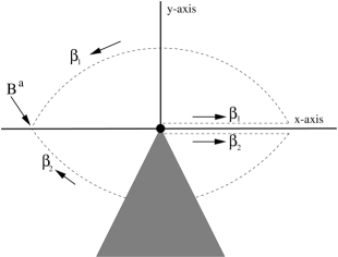
Figure 12: Particle sitting at rest in the origin

An observer traversing via path $\beta_{1}$ to the point $B^{a}$ would give this point different coordinates than an observer traversing path $\beta_{2}$. In the following we will choose coordinates in such a way that we remove the boundary conditions (i.e. we will have coordinates with the conventional ranges) but as a price we will generate a non trivial interaction term. If we denote by $u^{a}$ the flat multi-valued coordinates and by $x^{\mu}$ the curved, single-valued coordinates, the metric in terms if the $x^{\mu}$ becomes:

$$g_{\mu\nu}(x)=\frac{\partial}{\partial x^{\mu}}u^{a}(x)\frac{\partial}{\partial x^{\nu}}u^{b}(x)\eta_{ab}$$ (95)

First we like to choose a slicing condition. For that we view $u^{a}(x)$ as embedding coordinates. So for every time $t$ we want to define a function $u^{a}(x,y;t)$ that tells us how the $t=$constant surface is embedded in flat 3-dimensional Minkowski space-time. The condition will be that locally the area of the surface must be maximal. This is of course always possible which assures us that the gauge will be accessible. Actually it is precisely the Polyakov action used in string theory that should be maximalised:

$$S_{P}=\int d^{2}x~{}\sqrt{\gamma}\gamma^{ij}\partial_{i}u^{a}\partial_{j}u^{b}\eta_{ab}$$ (96)

On the Cauchy surface we will choose conformal, complex coordinates, i.e.:

$$\gamma_{ij}=e^{\phi}\delta_{ij}~{}~{}~{}~{}~{}~{}~{}z=x+iy~{}~{}~{}~{}~{}~{}~{}\bar{z}=x-iy$$ (97)

The Polyakov action then reduces to:

$$S_{P}=\int d^{2}z~{}\partial u^{a}\bar{\partial}u^{b}\eta_{ab}~{}~{}~{}~{}~{}\partial=\frac{\partial}{\partial z}~{}~{}~{}~{}~{}~{}\bar{\partial}=\frac{\partial}{\partial\bar{z}}$$ (98)

It is well known that the equations that follow from this action are:

$$\partial u^{a}\partial u^{b}\eta_{ab} = 0$$ (99)

$$\bar{\partial}u^{a}\bar{\partial}u^{b}\eta_{ab} = 0$$ (100)

$$\partial\bar{\partial}u^{a} = 0$$ (101)

So $u^{a}$ must be a harmonic function: $u^{a}=u^{a}(z;t)+u^{a}(\bar{z};t)$. We will try to solve the dreibein field $e^{~{}~{}a}_{\mu}=\partial_{\mu}u^{a}$ in the following. The conditions (99,100,101) translate into the following conditions for the dreibeins:

$$e^{~{}~{}a}_{0}\equiv\partial_{t}u^{a} = C^{a}(t)+\partial_{t}\int dz~{}e_{z}^{~{}~{}a}+\partial_{t}\int d\bar{z}~{}e_{\bar{z}}^{~{}~{}a}$$ (102)

$$e_{z}^{~{}~{}a}\equiv\partial u^{a} = e_{z}^{~{}~{}a}(z)~{}~{}~{}\mbox{(holomorphic)}$$ (103)

$$e_{\bar{z}}^{~{}~{}a}\equiv\bar{\partial}u^{a} = e_{\bar{z}}^{~{}~{}a}(\bar{z})~{}~{}~{}\mbox{(anti-holomorphic)}$$ (104)

$$e_{z}^{~{}~{}a}e_{z}^{~{}~{}b}\eta_{ab} = 0~{}~{}~{}~{}~{}~{}~{}~{}~{}~{}~{}\mbox{(null-vector)}$$ (105)

$$e_{\bar{z}}^{~{}~{}a}e_{\bar{z}}^{~{}~{}b}\eta_{ab} = 0~{}~{}~{}~{}~{}~{}~{}~{}~{}~{}~{}\mbox{(null-vector)}$$ (106)

where $C^{a}(t)$ is some vector only depending on t. Note that there is still conformal freedom: $z\rightarrow f(z)$. These conditions in turn can be translated into conditions on $\pi^{ij}$ and $\gamma_{ij}$ (for the definition of the canonical momentum $\pi^{ij}$ (see [1]):

$$\gamma_{ij}=e^{\phi}\delta_{ij}~{}~{}~{}~{}~{}~{}~{}~{}~{}~{}~{}\pi\equiv\pi^{i}_{i}=0$$ (107)

The advantage of these conditions is now evident. First of all, conditions (107) indeed imply that the kinetic term in the Einstein-Hilbert action ($\pi^{ij}\partial_{t}\gamma_{ij}$) vanishes. To see that, one must split $\pi^{ij}$ and $\gamma_{ij}$ into a traceless part and the trace. As $\pi$ is conjugate to ${\bf Tr}\gamma_{ij}=2e^{\phi}$ we find the result. Futhermore from a mathematical point of view it is very convenient that $e_{z}^{~{}~{}a}$ is a holomorphic vector because it allows us to use the machinery of complex calculus.

Next we will try to reduce the problem of solving the gravitational field around the moving particles to a mathematical problem, known as the Riemann-Hilbert problem. First we mention that all the information for the gravitational fields is really in $e_{z}^{~{}~{}a}$ and the asymptotic behaviour of the gravitational field at infinity. If we know $e_{z}^{~{}~{}a}$ and the boundary conditions at infinity we can in principle calculate $e_{\bar{z}}^{~{}~{}a}$ and $e_{0}^{~{}~{}a}$. The asymptotic behaviour can be studied by solving the gravitational field around a massive spinning particle in our gauge. We expect that at $z\rightarrow\infty$ this is the asymptotic form of the multiparticle solution. The total mass of the universe is the the mass of the particle and the total angular momentum is its spin (see [12]). We have already argued that the flat coordinates $u^{a}$ are multivalued if we traverse a loop around a particle. Specifically if we move around one particle the result will only depend on the first homotopy class of the punctured plane and not on the precise path chosen. The transformation will be:

$$u^{a}\stackrel{{\scriptstyle[\gamma_{i}]}}{{\rightarrow}}(B_{i}R_{i}B_{i}^{-1}\cdot u)^{a}+q_{i}^{a}$$ (108)

where $B_{i}$ is a boost-matrix, $R_{i}$ a rotation-matrix and $q_{i}^{a}$ is the translation-vector.$[\gamma_{i}]$ Denotes a loop in a certain class. We will look at the transformation properties of $e_{z}^{~{}~{}a}=\partial u^{a}$:

$$e_{z}^{~{}~{}a}\stackrel{{\scriptstyle[\gamma_{i}]}}{{\rightarrow}}(B_{i}R_{i}B^{-1}_{i}\cdot e_{z})^{a}$$ (109)

The Riemann-Hilbert problem is now formulated as follows:

Given these set of monodromy transformations ($M_{i}=B_{i}R_{i}B_{i}^{-1}$) on a Riemann surface, find the vector-functions $e_{z}^{~{}~{}a}$ that transform in this way if we move around the puncture.

Because of the multivaluedness of $e_{z}^{~{}~{}a}$ we need cuts in the plane from the $i^{th}$ puncture to infinity. $e_{z}^{~{}~{}a}$ Must now transform as it moves over the cut. The familiar 1-dimensional example is of course $f(z)=z^{\alpha}$ where $f\rightarrow e^{2\pi i\alpha}f$ as we cross the cut. To treat the R-H problem it is more convenient to use the 2 dimensional SU(1,1) representation which is the covering of SO(2,1). The R-H problem still remains the same only the monodromy matrices $M_{i}$ now live in SU(1,1). From the spinor solution to the R-H problem (denoted by $\zeta^{\alpha}$) we can then easily reconstruct the vector solution $e_{z}^{~{}~{}a}$. It is also important to mention that the metric is single-valued (as it should be).

$$g_{\mu\nu}=\eta_{ab}e^{~{}~{}a}_{\mu}e^{~{}~{}b}_{\nu}\rightarrow\eta_{ab}(M_{i}\cdot e_{\mu})^{a}(M_{i}\cdot e_{\nu})^{b}=g_{\mu\nu}$$ (110)

Here we used the orthogonality property of SO(2,1) matrices:

$$M^{a}_{~{}~{}b}M^{b}_{~{}~{}d}\eta_{ab}=\eta_{cd}$$ (111)

Another important remark is that the monodromy around the $z=\infty$ is determined by the other monodromies around $z=a_{i}$:

$$M_{\infty}^{-1}=M_{N}.....M_{1}$$ (112)

This is due to the fact that a loop around infinity (on the Riemann-sphere) is equivalent to a loop around all particles in the opposite direction.

There are 2 ways of studying the R-H problem and we will only briefly sketch the methods here. In one approach one tries to write down a d’th order differential equation with N+1 singularities (one of which is located at infinity). d Is the dimension used for the representation (d=2 for SU(1,1) and d=3 for SO(2,1)) and N is the number of particles involved. The singularities must be of the special type called ”regular singularities”. It is always possible by a global Lorentz transformation to go to a frame in which the $i^{th}$ particle is not moving. This then implies that the monodromy around that particle is given by a rotation. In this frame the spinor $\zeta^{\alpha}$ has the following singular behaviour near the particle:

$$\zeta^{\alpha}\stackrel{{\scriptstyle z\rightarrow a_{i}}}{{\sim}}(z-a_{i})^{\lambda^{\alpha}_{i}}[b^{\alpha}_{i}+c_{i}^{\alpha}(z-a_{i})+...]$$ (113)

where $\lambda^{\alpha}_{i}$ are called the local exponents. They must obey the following rule:

$$\sum_{\alpha=1}^{d}\sum_{k=1}^{N}\lambda^{\alpha}_{k}+\sum_{\alpha=1}^{d}\lambda^{\alpha}_{\infty}=\frac{d(d-1)}{2}(N-1)$$ (114)

In our case we will choose:

$$\lambda^{\alpha}_{i}=(-\frac{\alpha_{i}}{2},\frac{\alpha_{i}}{2})~{}~{}~{}~{}~{}~{}~{}~{}~{}\alpha_{i}=4Gm_{i}$$ (115)

for the singularities in the finite part of the plane. The exponents at infinity are then determined by relations (112,114). It is important to notice that changing the local exponents by integers will not change the monodromy. To solve the R-H problem uniquely we have to choose the monodromy and the integer part of the exponents independently. One argument to choose certain exponents could be that we demand that the singular behaviour matches the behaviour found in pertubative calculations (small $Gm$). From (113) we can easily deduce the the monodromy matrix:

$$M_{1}=\left(\begin{array}[]{cc}e^{-i\pi\alpha_{1}}&0\\ 0&e^{i\pi\alpha_{1}}\end{array}\right)~{}~{}~{}~{}~{}~{}~{}~{}~{}\alpha_{i}=4Gm_{i}$$ (116)

The difficulty is of course that not all monodromies commute and can be brought simultaneously to this diagonal form. For 2 particles however we can prove that the most general second order linear differential equation with 2 singularities and 1 at infinity can be written as a hypergeometric equation. It is long known that the 2 independent solutions of the hypergeometric equation transform into a linear combination of them if we traverse a path around a singularity. By matching this monodromy with the desired monodromy we can find a specific solution to the R-H problem [7, 25, 12].

For more than 2 particles it is convenient to to consider a (equivalent) linear, first order matrix differential equation of the form:

$$\partial Y=\sum_{i=1}^{N}Y\frac{A_{i}}{z-a_{i}}$$ (117)

$Y$ is the fundamental matrix of solutions to the differential equation. The matrices $A_{i}$ are not depending on $z$ (but may depend on $a_{i}$ !). We demand that the solutions to this equation must fullfill the following conditions:

1. $Y(z_{o})=I$

2. $Y(z)$ is holomorphic in $(C-\{a_{1}...a_{N},\infty\})$

3. $Y(z)$ has the following short distance behaviour near a singular point:

$$Y(z)\stackrel{{\scriptstyle z\rightarrow a_{i}}}{{\sim}}(z-a_{i})^{L_{i}}\hat{Y}_{i}(z)$$ (118)

where $M_{i}=e^{2\pi iL_{i}}$ and $M_{i}$ are the monodromy matrices. It is also important that the matrix $\hat{Y}_{i}(z)$ is holomorphic and invertable at $z=a_{i}$. So:

$$\hat{Y}_{i}(z)\stackrel{{\scriptstyle z\rightarrow a_{i}}}{{\sim}}(Y^{0}(a_{i})+Y^{1}(a_{i})(z-a_{i})+....)$$ (119)

with $\det|Y^{0}(a_{i})|\neq 0$. The R-H problem is now converted into finding the differential equation (117) or equivalently to find the matrices $A_{i}$. This problem is in principle solved in the mathematical literature [20, 21]. Lappo-Danilevsky found an explicit solution to this problem in terms of a series expansion in the $L_{i}$-matrices. He could prove convergence of this series for small enough $L_{i}$. We will however not go into this technical details of this solution. Miwa, Sato and Jimbo found a representation of the $Y(z,a_{i})$ in terms of a correlation function of conformal Dirac-spinors in a free field conformal field theory. The particles are represented by twistoperators and ensure the right monodromy properties if one moves around a particle. We refer the interested reader to the literature [26, 22, 23, 12].

5 Discussion

In this survey we discussed some ways of treating 2+1-gravity coupled to point-particles. We think this is an important issue because it is the starting point for a quantised theory of gravity. One could for instance be interested in defining a consistent S-matrix for quantised particles. First of all in- and out-states should be defined with great care because the interaction is long range. We expect however that consistent in- and outgoing states can be defined because exact stationary scaling solutions exist (i.e. all particles move for instance towards the center with a constant velocity proportional to the distance from the center). It is however not clear if for some incoming configurations the universe crunches and no outgoing states exist (or there may for instance exist bound states of particles). Ultimately one would like to be able to describe creation and annihilation of particles. Concluding we would like to say that a lot of interesting work lies ahead.

6 Acknowledgements

I would like to thank the organising comittee of the Kazan State University for their hospitality during my visit. Also I would like to thank the fellow Phd-student for their friendship.

References

- [1] Misner C W, Thorne K S and Wheeler J A 1973 Gravitation (San Francisco: W.H. Freeman and Company)
- [2] Staruszkiewicz A 1963 Acta Phys. Polon. 24 734
-
[3]
Deser S, Jackiw R and ’t Hooft G 1984
Ann. Phys. 152 220
Gott J R and Alpert M 1984 Gen. Rel. Grav. 16 243
Giddings S Abbot J and Kuchar K 1984 Gen. Rel. Grav. 16 751 - [4] Deser S and Jackiw R 1984 Ann. Phys. 153 405
-
[5]
’t Hooft G 1992 Class. Quant. Grav. 9 1335
’t Hooft G 1993 Class. Quant. Grav. 10 S79
’t Hooft G 1993 Class. Quant. Grav. 10 1023
’t Hooft G 1993 Class. Quant. Grav. 10 1653 -
[6]
Achucarro A and Townsend P 1986 Phys. Lett.
B180 85
Witten E 1988 Nucl. Phys. B331 46 -
[7]
Grignani G and Nardelli G 1992 Phys. Rev. D45 2719
Grignani G and Nardelli G 1992 Nucl. Phys. B370 491
Vaz C and Witten L 1992 Nucl. Phys. B368 509
Vaz C and Witten L 1992 Mod. Phys. Lett. A7 2763 - [8] Carlip S 1993 Canadian Gen. Rel. 1993 215
-
[9]
Mazur P O 1986 Phys. Rev. Lett. 57 929
Mazur P O 1987 Phys. Rev. Lett. 59 2380
’t Hooft G 1988 Comm. Math. Phys. 117 685
Deser S and Jackiw R 1988 Comm. Math. Phys. 118 495
de Sousa Gerbert P and Jackiw R 1989 Comm. Math. Phys. 124 229 -
[10]
Carlip S 1989 Nucl. Phys. B324 106
Koehler K, Mansouri, Vaz C and Witten L 1991 Nucl. Phys B348 373 - [11] Ashtekar A and Varadarajan M 1994 Phys. Rev. D50 4944
- [12] Welling M. 1995 Gravity in (2+1)-dimensions as a Riemann-Hilbert problem Preprint THU-95-24
-
[13]
Loll R 1995 Quantum aspects of 2+1 gravity Preprint DFF
233/03/95
Carlip S 1995 Lectures on (2+1)-dimensional gravity Preprint UCD-95-6 -
[14]
Waelbroeck H 1990 Class. Quant. Grav. 7 751
Waelbroeck H 1991 Nucl. Phys. B364 475
Waelbroeck H 1994 Phys. Rev. D50 4982 - [15] Clément G 1985 Int. J. Theor. Phys. 24 852
- [16] Kohler C 1995 Class. Quant. Grav. 12 L11
- [17] Regge T and Teitelboim C 1974 Ann. Phys. 88 286
- [18] Henneaux M 1984 Phys. Rev. D29 2766
- [19] Martin S P 1989 Nucl. Phys. B327 178
- [20] Plemelj J 1964 Problems in the sense of Riemann and Klein (London: John Wiley)
-
[21]
Chudnovsky D V 1979 in Bifurcation phenomena in
mathematical physics and related topics Bardos C and Bessis P (eds.) pp. 385
(Dordrecht: D. Reidel Publishing Company)
Chudnovsky G V 1979 in Complex Analysis, Microcalculus, and Relastivistic Quantum Theory Lagolnitzer D (ed.) Lecture notes in physics 120 (New York: Berlin Springer Verlag) - [22] Sato M, Miwa T and Jimbo M 1979 in Complex Analysis, Microcalculus, and Relastivistic Quantum Theory Lagolnitzer D (ed.) Lecture notes in physics 120 (New York: Berlin Springer Verlag)
- [23] Blok B and Yankielowicz S 1989 Nucl. Phys. B321 717
- [24] Sansone G. and Gerretsen 1969 Lectures on the theory of functions of a complex variable II (Groningen: Wolters- Noordhoff)
-
[25]
Bellini A, Ciafaloni M and Valtancoli 1995 (2+1)-Gravity
with
moving particles in an instantaneous gauge Preprint: CERN-TH/95-192
Bellini A, Ciafaloni M and Valtancoli 1995 Non-perturbative particle dynamics in (2+1)-gravity Preprint CERN-TH/95-193
Bellini A, Ciafaloni M and Valtancoli P 1995 Phys. Lett. B348 44 - [26] Moore G 1990 Comm. Math. Phys. 133 261
-
[27]
Ashtekar A 1987 Phys. Rev. D36 1587
Rovelli C and Smolin L 1990 Nucl. Phys. B331 80