November 1995 PAR–LPTHE 95-46, ITFA-95-20, hep-th/9511201
DISCRETE GAUGE THEORIES

Abstract

In these lecture notes, we present a self-contained treatment of planar gauge theories broken down to some finite residual gauge group $H$ via the Higgs mechanism. The main focus is on the discrete $H$ gauge theory describing the long distance physics of such a model. The spectrum features global $H$ charges, magnetic vortices and dyonic combinations. Due to the Aharonov-Bohm effect, these particles exhibit topological interactions. Among other things, we review the Hopf algebra related to this discrete $H$ gauge theory, which provides an unified description of the spin, braid and fusion properties of the particles in this model. Exotic phenomena such as flux metamorphosis, Alice fluxes, Cheshire charge, (non)abelian braid statistics, the generalized spin-statistics connection and nonabelian Aharonov-Bohm scattering are explained and illustrated by representative examples.

Broken symmetry revisited

Symmetry has become one of the major guiding principles in physics during the twentieth century. Over the past ten decades, we have gradually progressed from external to internal, from global to local, from finite to infinite, from ordinary to supersymmetry and quite recently arrived at the notion of Hopf algebras or quantum groups.

In general, a physical system consists of a finite or infinite number of degrees of freedom which may or may not interact. The dynamics is prescribed by a set of evolution equations which follow from varying the action with respect to the different degrees of freedom. A symmetry then corresponds to a group of transformations on the space time coordinates and/or the degrees of freedom that leave the action and therefore also the evolution equations invariant. External symmetries have to do with invariances (e.g. Lorentz invariance) under transformations on the space time coordinates. Symmetries not related to transformations of space time coordinates are called internal symmetries. We also discriminate between global symmetries and local symmetries. A global or rigid symmetry transformation is the same throughout space time and usually leads to a conserved quantity. Turning a global symmetry into a local symmetry, i.e. allowing the symmetry transformations to vary continuously from one point in space time to another, requires the introduction of additional gauge degrees of freedom mediating a force. It is this so-called gauge principle that has eventually led to the extremely successful standard model of the strong and electro-weak interactions between the elementary particles based on the local gauge group $SU(3)\times SU(2)\times U(1)$.

The use of symmetry considerations has been extended significantly by the observation that a symmetry of the action is not automatically a symmetry of the groundstate of a physical system. If the action is invariant under some symmetry group $G$ and the groundstate only under a subgroup $H$ of $G$, the symmetry group $G$ is said to be spontaneously broken down to $H$. The symmetry is not completely lost though, for the broken generators of $G$ transform one groundstate into another.

The physics of a broken global symmetry is quite different from a broken local (gauge) symmetry. The signature of a broken continuous global symmetry group $G$ in a physical system is the occurrence of massless scalar degrees of freedom, the so-called Goldstone bosons. Specifically, each broken generator of $G$ gives rise to a massless Goldstone boson field. Well-known realizations of Goldstone bosons are the long range spin waves in a ferromagnet, in which the rotational symmetry is broken below the Curie temperature through the appearance of spontaneous magnetization. An application in particle physics is the low energy physics of the strong interactions, where the spontaneous breakdown of (approximate) chiral symmetry leads to (approximately) massless pseudoscalar particles such as the pions.

In the case of a broken local (gauge) symmetry, in contrast, the would be massless Goldstone bosons conspire with the massless gauge fields to form massive vector fields. This celebrated phenomenon is known as the Higgs mechanism. The canonical example in condensed matter physics is the ordinary superconductor. In the phase transition from the normal to the superconducting phase, the $U(1)$ gauge symmetry is spontaneously broken to the finite cyclic group ${\bf Z}_{2}$ by a condensate of Cooper pairs. This leads to a mass $M_{A}$ for the photon field in the superconducting medium as witnessed by the Meissner effect: magnetic fields are expelled from a superconducting region and have a characteristic penetration depth which in proper units is just the inverse of the photon mass $M_{A}$. Moreover, the Coulomb interactions among external electric charges in a superconductor are of finite range $\sim 1/M_{A}$. The Higgs mechanism also plays a key role in the unified theory of weak and electromagnetic interactions, that is, the Glashow-Weinberg-Salam model where the product gauge group $SU(2)\times U(1)$ is broken to the $U(1)$ subgroup of electromagnetism. In this context, the massive vector particles correspond to the $W$ and $Z$ bosons mediating the short range weak interactions. More speculative applications of the Higgs mechanism are those where the standard model of the strong, weak and electromagnetic interactions is embedded in a grand unified model with a large simple gauge group. The most ambitious attempts invoke supersymmetry as well.

In addition to the aforementioned characteristics in the spectrum of fundamental excitations, there are in general other fingerprints of a broken symmetry in a physical system. These are usually called topological excitations or just defects and correspond to collective degrees of freedom carrying ‘charges’ or quantum numbers which are conserved for topological reasons, not related to a manifest symmetry of the action. (See, for example, the references [cola, mermin, presbook, raja] for reviews). It is exactly the appearance of these topological charges which renders the corresponding collective excitations stable. Topological excitations may manifest themselves as particle-like, string-like or planar-like objects (solitons), or have to be interpreted as quantum mechanical tunneling processes (instantons). Depending on the model in which they occur, these excitations carry evocative names like kinks, domain walls, vortices, cosmic strings, Alice strings, monopoles, skyrmions, texture, sphalerons and so on. Defects are crucial for a full understanding of the physics of systems with a broken symmetry and lead to a host of rather unexpected and exotic phenomena which are in general of a nonperturbative nature.

The prototypical example of a topological defect is the Abrikosov-Nielsen-Olesen flux tube in the type II superconductor with broken $U(1)$ gauge symmetry [abri, niels]. The topologically conserved quantum number characterizing these defects is the magnetic flux, which indeed can only take discrete values. A beautiful but unfortunately not yet observed example in particle physics is the ’t Hooft-Polyakov monopole [thooftmon, polyamon] occurring in any grand unified model in which a simple gauge group $G$ is broken to a subgroup $H$ containing the electromagnetic $U(1)$ factor. Here, it is the quantized magnetic charge carried by these monopoles that is conserved for topological reasons. In fact, the discovery that these models support magnetic monopoles reconciled the two well-known arguments for the quantization of electric charge, namely Dirac’s argument based on the existence of a magnetic monopole [dirac] and the obvious fact that the $U(1)$ generator should be compact as it belongs to a larger compact gauge group.

An example of a model with a broken global symmetry supporting topological excitations is the effective sigma model describing the low energy strong interactions for the mesons. That is, the phase with broken chiral symmetry mentioned before. One may add a topological term and a stabilizing term to the action and obtain a theory that features topological particle-like objects called skyrmions, which have exactly the properties of the baryons. See reference [skyrme] and also [fink, witsk]. So, upon extending the effective model for the Goldstone bosons, we recover the complete spectrum of the underlying strong interaction model (quantum chromodynamics) and its low energy dynamics. Indeed, this picture leads to an attractive phenomenological model for baryons.

Another area of physics where defects may play a fundamental role is cosmology. See for instance reference [brand] for a recent review. According to the standard cosmological hot big bang scenario, the universe cooled down through a sequence of local and/or global symmetry breaking phase transitions in a very early stage. The question of the actual formation of defects in these phase transitions is of prime importance. It has been argued, for instance, that magnetic monopoles might have been produced copiously. As they tend to dominate the mass in the universe, however, magnetic monopoles are notoriously hard to accommodate and if indeed formed, they have to be ‘inflated away’. Phase transitions that see the production of (local or global) cosmic strings, on the other hand, are much more interesting. In contrast with magnetic monopoles, the presence of cosmic strings does not lead to cosmological disasters and according to an attractive but still speculative theory cosmic strings may even have acted as seeds for the formation of galaxies and other large scale structures in the present day universe.

Similar symmetry breaking phase transitions are extensively studied in condensed matter physics. We have already mentioned the transition from the normal to the superconducting phase in superconducting materials of type II, which may give rise to the formation of magnetic flux tubes. In the field of low temperature physics, there also exists a great body of both theoretical and experimental work on the transitions from the normal to the many superfluid phases of helium-3 in which line and point defects arise in a great variety, e.g. [volovik]. Furthermore, in uniaxial nematic liquid crystals, point defects, line defects and texture arise in the transition from the disordered to the ordered phase in which the rotational global symmetry group $SO(3)$ is broken down to the semi-direct product group $U(1)\times_{\rm s.d.}{\bf Z}_{2}$. Bi-axial nematic crystals, in turn, exhibit a phase transition in which the global rotational symmetry group is broken down to the product group ${\bf Z}_{2}\times{\bf Z}_{2}$ yielding line defects labeled by the elements of the (nonabelian) quaternion group $\bar{D}_{2}$, e.g. [mermin]. Nematic crystals are cheap materials and as compared to helium-3, for instance, relatively easy to work with in the laboratory. The symmetry breaking phase transitions typically appear at temperatures that can be reached by a standard kitchen oven, whereas the size of the occurring defects is such that these can be seen by means of a simple microscope. Hence, these materials form an easily accessible experimental playground for the investigation of defect producing phase transitions and as such may partly mimic the physics of the early universe in the laboratory. For some recent ingenious experimental studies on the formation and the dynamics of topological defects in nematic crystals making use of high speed film cameras, the interested reader is referred to [bowick, turok].

From a theoretical point of view, many aspects of topological defects have been studied and understood. At the classical level, one may roughly sketch the following programme. One first uses simple topological arguments, usually of the homotopy type, to see whether a given model does exhibit topological charges. Subsequently, one may try to prove the existence of the corresponding classical solutions by functional analysis methods or just by explicit construction of particular solutions. On the other hand, one may in many cases determine the dimension of the solution or moduli space and its dependence on the topological charge using index theory. Finally, one may attempt to determine the general solution space more or less explicitly. In this respect, one has been successful in varying degree. In particular, the self-dual instanton solutions of Yang-Mills theory on $S^{4}$ have been obtained completely.

The physical properties of topological defects can be probed by their interactions with the ordinary particles or excitations in the model. This amounts to investigating (quantum) processes in the background of the defect. In particular, one may calculate the one-loop corrections to the various quantities characterizing the defect, which involves studying the fluctuation operator. Here, one naturally has to distinguish the modes with zero eigenvalue from those with nonzero eigenvalues. The nonzero modes generically give rise to the usual renormalization effects, such as mass and coupling constant renormalization. The zero modes, which often arise as a consequence of the global symmetries in the theory, lead to collective coordinates. Their quantization yields a semiclassical description of the spectrum of the theory in a given topological sector, including the external quantum numbers of the soliton such as its energy and momentum and its internal quantum numbers such as its electric charge, e.g. [cola, presbook].

In situations where the residual gauge group $H$ is nonabelian, the analysis outlined in the previous paragraph is rather subtle. For instance, the naive expectation that a soliton can carry internal electric charges which form representations of the complete unbroken group $H$ is wrong. As only the subgroup of $H$ which commutes with the topological charge can be globally implemented, these internal charges form representations of this so-called centralizer subgroup. (See [balglob, nelson, nelsonc] for the case of magnetic monopoles and [spm, balglob2] for the case of magnetic vortices). This makes the full spectrum of topological and ordinary quantum numbers in such a broken phase rather intricate.

Also, an important effect on the spectrum and the interactions of a theory with a broken gauge group is caused by the introduction of additional topological terms in the action, such as a nonvanishing $\theta$ angle in 3+1 dimensional space time and the Chern-Simons term in 2+1 dimensions. It has been shown by Witten that in case of a nonvanishing $\theta$ angle, for example, magnetic monopoles carry electric charges which are shifted by an amount proportional to $\theta/2\pi$ and their magnetic charge [thetaw].

Other results are even more surprising. A broken gauge theory only containing bosonic fields may support topological excitations (dyons), which on the quantum level carry half-integral spin and are fermions, thereby realizing the counterintuitive possibility to make fermions out of bosons [thora, jare]. It has subsequently been argued by Wilczek [wilcchfl] that in 2+1 dimensional space time one can even have topological excitations, namely flux/charge composites, which behave as anyons [leinaas], i.e. particles with fractional spin and quantum statistics interpolating between bosons and fermions. The possibility of anyons in two spatial dimensions is not merely of academic interest, as many systems in condensed matter physics, for example, are effectively described by 2+1 dimensional models. Indeed, anyons are known to be realized as quasiparticles in fractional quantum Hall systems [hal, laugh]. Further, it has been been shown that an ideal gas of electrically charged anyons is superconducting [chen, fetter, laughsup, anyonbook]. At present it is unclear whether this new and rather exotic type of superconductivity is actually realized in nature.

Furthermore, remarkable calculations by ’t Hooft revealed a nonperturbative mechanism for baryon decay in the standard model through instantons and sphalerons [thooftinst]. Afterwards, Rubakov and Callan discovered the phenomenon of baryon decay catalysis induced by grand unified monopoles [callan, ruba]. Baryon number violating processes also occur in the vicinity of grand unified cosmic strings as has been established by Alford, March-Russell and Wilczek [alfbar].

So far, we have given a (rather incomplete) enumeration of properties and processes that involve the interactions between topological and ordinary excitations. However, the interactions between defects themselves can also be highly nontrivial. Here, one should not only think of ordinary interactions corresponding to the exchange of field quanta. Consider, for instance, the case of Alice electrodynamics which occurs if some nonabelian gauge group (e.g. $SO(3)$) is broken to the nonabelian subgroup $U(1)\times_{\rm s.d.}{\bf Z}_{2}$, that is, the semi-direct product of the electromagnetic group $U(1)$ and the additional cyclic group ${\bf Z}_{2}$ whose nontrivial element reverses the sign of the electromagnetic fields [schwarz]. This model features magnetic monopoles and in addition a magnetic ${\bf Z}_{2}$ string (the so-called Alice string) with the miraculous property that if a monopole (or an electric charge for that matter) is transported around the string, its charge will change sign. In other words, a particle is converted into its own anti-particle. This nonabelian analogue of the celebrated Aharonov-Bohm effect [ahabo] is of a topological nature. That is, it only depends on the number of times the particle winds around the string and is independent of the distance between the particle and the string.

Similar phenomena occur in models in which a continuous gauge group is spontaneously broken down to some finite subgroup $H$. The topological defects supported by such a model are string-like in three spatial dimensions and carry a magnetic flux corresponding to an element $h$ of the residual gauge group $H$. As these string-like objects trivialize one spatial dimension, we may just as well descend to the plane, for convenience. In this arena, these defects become magnetic vortices, i.e. particle-like objects of characteristic size $1/M_{H}$ with $M_{H}$ the symmetry breaking scale. Besides these topological particles, the broken phase features matter charges labeled by the unitary irreducible representations $\Gamma$ of the residual gauge group $H$. Since all gauge fields are massive, there are no ordinary long range interactions among these particles. The remaining long range interactions are topological Aharonov-Bohm interactions. If the residual gauge group $H$ is nonabelian, for instance, the nonabelian fluxes $h\in H$ carried by the vortices exhibit flux metamorphosis [bais]. In the process of circumnavigating one vortex with another vortex their fluxes may change. Moreover, if a charge corresponding to some representation $\Gamma$ of $H$ is transported around a vortex carrying the magnetic flux $h\in H$, it returns transformed by the matrix $\Gamma(h)$ assigned to the element $h$ in the representation $\Gamma$ of $H$.

The spontaneously broken 2+1 dimensional models just mentioned will be the subject of these lecture notes. One of our aims is to show that the long distance physics of such a model is, in fact, governed by a Hopf algebra or quantum group based on the residual finite gauge group $H$ [spm, spm1, sm, thesis]. This algebraic framework manifestly unifies the topological and nontopological quantum numbers as dual aspects of a single symmetry concept. The results presented here strongly suggests that revisiting the symmetry breaking concept in general will reveal similar underlying algebraic structures.

The outline of these notes, which are intended to be accessible to a reader with a minimal background in field theory, quantum mechanics and finite group theory, is as follows. In chapter 1, we start with a review of the basic physical properties of a planar gauge theory broken down to a finite gauge group via the Higgs mechanism. The main focus will be on the discrete $H$ gauge theory describing the long distance of such a model. We argue that in addition to the aforementioned magnetic vortices and global $H$ charges the complete spectrum also consists of dyonic combinations of the two and establish the basic topological interactions among these particles. In chapter 2, we then turn to the Hopf algebra related to this discrete $H$ gauge theory and elaborate on the unified description this framework gives of the spin, braid and fusion properties of the particles. Finally, the general formalism developed in the foregoing chapters is illustrated by an explicit nonabelian example in chapter 3, namely a planar gauge theory spontaneously broken down to the double dihedral gauge group $\bar{D}_{2}$. Among other things, exotic phenomena like Cheshire charge, Alice fluxes, nonabelian braid statistics and nonabelian Aharonov-Bohm scattering are explained there.

Let us conclude this preface with some remarks on conventions. Throughout these notes units in which $\hbar=c=1$ are employed. Latin indices take the values $1,2$. Greek indices run from $0$ to $2$. Further, $x^{1}$ and $x^{2}$ denote spatial coordinates and $x^{0}=t$ the time coordinate. The signature of the three dimensional metric is taken as $(+,-,-)$. Unless stated otherwise, we adopt Einstein’s summation convention.

Chapter 1 Basics

1.1 Introduction

The planar gauge theories we will study in these notes are given by an action of the general form

$$S = S_{\rm YMH}+S_{\rm matter}.$$ (1.1.1)

The continuous gauge group $G$ of this model is assumed to be broken down to some finite subgroup $H$ of $G$ by means of the Higgs mechanism. That is, the Yang-Mills Higgs part $S_{\rm YMH}$ of the action features a Higgs field whose nonvanishing vacuum expectation values are only invariant under the action of $H$. Further, the matter part $S_{\rm matter}$ describes matter fields covariantly coupled to the gauge fields. A discussion of the implications of adding a Chern-Simons term to the spontaneously broken planar gauge theory (1.1.1) is beyond the scope of these notes. For this, the interested reader is referred to [spm1, sm, sam, thesis].

Since the unbroken gauge group $H$ is finite, all gauge fields are massive and it seems that the low energy or equivalently the long distance physics of the model (1.1.1) is trivial. This is not the case though. It is the occurrence of topological defects and the persistence of the Aharonov-Bohm effect that renders the long distance physics nontrivial. Specifically, the defects supported by these models are (particle-like) vortices of characteristic size $1/M_{H}$, with $M_{H}$ the symmetry breaking scale. These vortices carry magnetic fluxes labeled by the elements $h$ of the residual gauge group $H$.  In other words, the vortices introduce nontrivial holonomies in the locally flat gauge fields. Consequently, if the residual gauge group ${H}$ is nonabelian, these fluxes exhibit nontrivial topological interactions: in the process in which one vortex circumnavigates another, the associated magnetic fluxes feel each others’ holonomies and affect each other through conjugation. This is in a nutshell the long distance physics described by the Yang-Mills Higgs part $S_{\rm YMH}$ of the action. The matter fields, covariantly coupled to the gauge fields in the matter part $S_{\rm matter}$ of the action, form multiplets which transform irreducibly under the broken gauge group ${G}$. In the broken phase, these branch to irreducible representations of the residual gauge group ${H}$. So, the matter fields introduce point charges in the broken phase labeled by the unitary irreducible representations $\Gamma$ of $H$. When such a charge encircles a magnetic flux $h\in H$, it undergoes an Aharonov-Bohm effect: it returns transformed by the matrix $\Gamma(h)$ assigned to the group element $h$ in the representation $\Gamma$ of $H$.

In this chapter, we establish the complete spectrum of the discrete $H$ gauge theory describing the long distance physics of the spontaneously broken model (1.1.1), which besides the aforementioned matter charges and magnetic vortices also consists of dyons obtained by composing these charges and vortices. In addition, we elaborate on the basic topological interactions between these particles. The discussion is organized as follows. In section 1.2, we start by briefly recalling that particle interchanges in the plane are organized by braid groups. Section 1.3 then contains an analysis of a planar abelian Higgs model in which the $U(1)$ gauge group is spontaneously broken to the cyclic subgroup ${\bf Z}_{N}$. The main emphasis will be on the ${\bf Z}_{N}$ gauge theory that describes the long distance physics of this model. Among other things, we show that the spectrum indeed consists of ${\bf Z}_{N}$ fluxes, ${\bf Z}_{N}$ charges and dyonic combinations of the two, establish the quantum mechanical Aharonov-Bohm interactions between these particles and argue that as a result the wave functions of the multi-particle configurations in this model realize nontrivial abelian representations of the related braid group. Finally, the subtleties involved in the generalization to models in which a nonabelian gauge group $G$ is broken to a nonabelian finite group $H$ are dealt with in section 1.4.

1.2 Braid groups

Let us consider a system of $n$ indistinguishable particles moving on a manifold $M$, which is assumed to be connected and path connected for convenience. The classical configuration space of this system is given by

$${\cal C}_{n}({M}) = (M^{n}-D)/S_{n},$$ (1.2.1)

where the action of the permutation group $S_{n}$ on the particle positions is divided out to account for the indistinguishability of the particles. Moreover, the singular configurations $D$ in which two or more particles coincide are excluded. The configuration space (1.2.1) is in general multiply-connected. This means that there are different kinematical options to quantize this multi-particle system. To be precise, there is a quantization associated to each unitary irreducible representation (UIR) of the fundamental group $\pi_{1}({\cal C}_{n}({M}))$. See, for instance, the references [imma, laid, schul, schul2].

It is easily verified that for manifolds $M$ with dimension larger then 2, we have the isomorphism $\pi_{1}({\cal C}_{n}({M}))\simeq S_{n}$. Hence, the inequivalent quantizations of multi-particle systems moving on such manifolds are labeled by the UIR’s of the permutation group $S_{n}$. There are two 1-dimensional UIR’s of $S_{n}$. The trivial representation naturally corresponds with Bose statistics. In this case, the system is quantized by a (scalar) wave function, which is symmetric under all permutations of the particles. The anti-symmetric representation, on the other hand, corresponds with Fermi statistics, i.e. we are dealing with a wave function which acquires a minus sign under odd permutations of the particles. Finally, parastatistics is also conceivable. In this case, the system is quantized by a multi-component wave function which transforms as a higher dimensional UIR of $S_{n}$.

Figure 1.1: The braid operator $\tau_{i}$ establishes a counterclockwise interchange of the particles $i$ and $i+1$ in a set of $n$ numbered indistinguishable particles in the plane.

It has been known for some time that quantum statistics for identical particles moving in the plane ($M={\bf R}^{2}$) can be much more exotic then in three or more dimensions [leinaas, wilcan]. The point is that the fundamental group of the associated configuration space ${\cal C}_{n}({\bf R}^{2})$ is not given by the permutation group, but rather by the so-called braid group $B_{n}({\bf R}^{2})$ [wu]. In contrast with the permutation group $S_{n}$, the braid group $B_{n}({\bf R}^{2})$ is a nonabelian group of infinite order. It is generated by $n-1$ elements $\tau_{1},\ldots,\tau_{n-1}$, where $\tau_{i}$ establishes a counterclockwise interchange of the particles $i$ and $i+1$ as depicted in figure 1.1. These generators are subject to the relations

$$\begin{array}[]{rcll}\tau_{i}\tau_{i+1}\tau_{i}&=&\tau_{i+1}\tau_{i}\tau_{i+1}&\qquad i=1,\ldots,n-2\\ \tau_{i}\tau_{j}&=&\tau_{j}\tau_{i}&\qquad|i-j|\geq 2,\end{array}$$ (1.2.4)

which can be presented graphically as in figure 1.2 and 1.3 respectively. In fact, the permutation group $S_{n}$ ruling the particle exchanges in three or more dimensions, is given by the same set of generators with relations (1.2.4) and the additional relations $\tau_{i}^{2}=e$ for all $i\in 1,\ldots,n-1$. These last relations are absent for $\pi_{1}({\cal C}_{n}({\bf R}^{2}))\simeq B_{n}({\bf R}^{2})$, since in the plane a counterclockwise particle interchange $\tau_{i}$ ceases to be homotopic to the clockwise interchange $\tau_{i}^{-1}$.

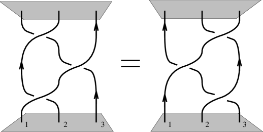
Figure 1.2: Pictorial presentation of the braid relation $\tau_{1}\tau_{2}\tau_{1}=\tau_{2}\tau_{1}\tau_{2}$. The particle trajectories corresponding to the composition of exchanges $\tau_{1}\tau_{2}\tau_{1}$ (diagram at the l.h.s.) can be continuously deformed into the trajectories associated with the composition of exchanges $\tau_{2}\tau_{1}\tau_{2}$ (r.h.s. diagram).

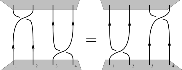
Figure 1.3: The braid relation $\tau_{1}\tau_{3}=\tau_{3}\tau_{1}$ expresses the fact that the particle trajectories displayed in the l.h.s. diagram can be continuously deformed into the trajectories in the r.h.s. diagram.

The one dimensional UIR’s of the braid group $B_{n}({\bf R}^{2})$ are labeled by an angular parameter $\Theta\in[0,2\pi)$ and are defined by assigning the same phase factor to all generators. That is,

$$\tau_{i} \mapsto \exp(\imath\Theta),$$ (1.2.5)

for all $i\in 1,\ldots,n-1$. The quantization of a system of $n$ identical particles in the plane corresponding to an arbitrary but fixed $\Theta\in[0,2\pi)$ is then given by a multi-valued (scalar) wave function that generates the quantum statistical phase $\exp(\imath\Theta)$ upon a counterclockwise interchange of two adjacent particles. For $\Theta=0$ and $\Theta=\pi$, we are dealing with bosons and fermions respectively. The particle species related to other values of $\Theta$ have been called anyons [wilcan]. Quantum statistics deviating from conventional permutation statistics is known under various names in the literature, e.g. fractional statistics, anyon statistics and exotic statistics. We adopt the following nomenclature. An identical particle system described by a (multi-valued) wave function that transforms as an one dimensional (abelian) UIR of the braid group $B_{n}({\bf R}^{2})$ ($\Theta\neq 0,\pi$) is said to realize abelian braid statistics. If an identical particle system is described by a multi-componenent wave function carrying an higher dimensional UIR of the braid group, then the particles are said to obey nonabelian braid statistics.

A system of $n$ distinguishable particles moving in the plane, in turn, is described by the non-simply connected configuration space

$${\cal Q}_{n}({\bf R}^{2}) = ({\bf R}^{2})^{n}-D.$$ (1.2.6)

The fundamental group of this configuration space is the so-called colored braid group $P_{n}({\bf R}^{2})$, also known as the pure braid group. The colored braid group $P_{n}({\bf R}^{2})$ is the subgroup of the ordinary braid group $B_{n}({\bf R}^{2})$ generated by the monodromy operators

$$\gamma_{ij} := \tau_{i}\cdots\tau_{j-2}\tau_{j-1}^{2}\tau_{j-2}^{-1}\cdots\tau_{i}^{-1}\qquad\qquad\mbox{with}\;1\leq i<j\leq n.$$ (1.2.7)

Here, the $\tau_{i}$’s are the generators of $B_{n}({\bf R}^{2})$ acting on the set of $n$ numbered distinguishable particles as displayed in figure 1.1. It then follows from the definition (1.2.7) that the monodromy operator $\gamma_{ij}$ takes particle $i$ counterclockwise around particle $j$ as depicted in figure 1.4. The different UIR’s of $P_{n}({\bf R}^{2})$ now label the inequivalent ways to quantize a system of $n$ distinguishable particles in the plane. Finally, a planar system that consists of a subsystem of identical particles of one type, a subsystem of identical particles of another type and so on, is of course also conceivable. The fundamental group of the configuration space of such a system is known as a partially colored braid group. Let the total number of particles of this system again be $n$, then the associated partially colored braid group is the subgroup of the ordinary braid group $B_{n}({\bf R}^{2})$ generated by the braid operators that interchange identical particles and the monodromy operators acting on distinguishable particles. See for example [brekfa, brekke].

Figure 1.4: The monodromy operator $\gamma_{ij}$ takes particle $i$ counterclockwise around particle $j$.

To conclude, the fundamental excitations in planar discrete gauge theories, namely magnetic vortices and matter charges, are in principle bosons. As will be argued in the next sections, in the first quantized description, these particles acquire braid statistics through the Aharonov-Bohm effect. Hence, depending on whether we are dealing with a system of identical particles, a system of distinguishable particles or a mixture, the associated multi-particle wave function generically transforms as a nontrivial representation of the ordinary braid group, colored braid group or partially colored braid group respectively.

1.3 ${\bf Z}_{N}$ gauge theory

The simplest example of a broken gauge theory is an $U(1)$ gauge theory spontaneously broken down to the cyclic subgroup ${\bf Z}_{N}$. This symmetry breaking scheme occurs in an abelian Higgs model in which the field that condenses carries charge $Ne$, with $e$ the fundamental charge unit [krawil]. The case $N=2$ is in fact realized in the ordinary BCS superconductor, as the field that condenses in the BCS superconductor is that associated with the Cooper pair carrying charge $2e$.

This section is devoted to a discussion of such an abelian Higgs model in 2+1 dimensional space time. We focus on the ${\bf Z}_{N}$ gauge theory describing the long range physics. The organization is as follows. In section 1.3.1, we will start with a brief review of the screening mechanism for the electromagnetic fields of external matter charges $q$ in the Higgs phase. We will argue that the external matter charges, which are multiples of the fundamental charge $e$ rather then multiples of the Higgs charge $Ne$, are surrounded by screening charges provided by the Higgs condensate. These screening charges screen the electromagnetic fields around the external charges. Thus, no long range Coulomb interactions persist among the external charges. The main point of section 1.3.2 will be, however, that the screening charges do not screen the Aharonov-Bohm interactions between the external charges and the magnetic vortices, which also feature in this model. As a consequence, long range Aharonov-Bohm interactions persist between the vortices and the external matter charges in the Higgs phase. Upon circumnavigating a magnetic vortex (carrying a flux $\phi$ which is a multiple of the fundamental flux unit $\frac{2\pi}{Ne}$ in this case) with an external charge $q$ (being a multiple of the fundamental charge unit $e$) the wave function of the system picks up the Aharonov-Bohm phase $\exp(\imath q\phi)$. These Aharonov-Bohm phases lead to observable low energy scattering effects from which we conclude that the physically distinct superselection sectors in the Higgs phase can be labeled as $(a,n)$, where $a$ stands for the number of fundamental flux units $\frac{2\pi}{Ne}$ and $n$ for the number of fundamental charge units $e$. In other words, the spectrum of the ${\bf Z}_{N}$ gauge theory in the Higgs phase consists of pure charges $n$, pure fluxes $a$ and dyonic combinations. Given the remaining long range Aharonov-Bohm interactions, these charge and flux quantum numbers are defined modulo $N$. Having identified the spectrum and the long range interactions as the topological Aharonov-Bohm effect, we proceed with a closer examination of this ${\bf Z}_{N}$ gauge theory in section 1.3.3. It will be argued that multi-particle systems in general satisfy abelian braid statistics. That is, the wave functions realize one dimensional representations of the associated braid group. In particular, identical dyons behave as anyons. We will also discuss the composition rules for the charge/flux quantum numbers when two particles are brought together. A key result of this section is a topological proof of the spin-statistics connection for the particles in the spectrum. This proof is of a general nature and applies to all the theories that will be discussed in these notes.

1.3.1 Coulomb screening

The planar abelian Higgs model which we will study is governed by the following action

$$S = \int d\,^{3}x\;({\cal L}_{\rm YMH}+{\cal L}_{\rm matter})$$ (1.3.1)

$${\cal L}_{\rm YMH} = -\frac{1}{4}F^{\kappa\nu}F_{\kappa\nu}+({\cal D}^{\kappa}\Phi)^{*}{\cal D}_{\kappa}\Phi-V(|\Phi|)$$ (1.3.2)

$${\cal L}_{\rm matter} = -j^{\kappa}A_{\kappa}.$$ (1.3.3)

The Higgs field $\Phi$ is assumed to carry the charge $Ne$ w.r.t. the compact $U(1)$ gauge symmetry. In the conventions we will adopt in these notes, this means that the covariant derivative reads ${\cal D}_{\rho}\Phi=(\partial_{\rho}+\imath NeA_{\rho})\Phi$. Furthermore, the potential

$$V(|\Phi|) = \frac{\lambda}{4}(|\Phi|^{2}-v^{2})^{2}\qquad\qquad\lambda,v>0,$$ (1.3.4)

endows the Higgs field with a nonvanishing vacuum expectation value $|\langle\Phi\rangle|=v$, which implies that the global continuous $U(1)$ symmetry is spontaneously broken. However, in this particular model the symmetry is not completely broken. Under global symmetry transformations $\Lambda(\alpha)$, with $\alpha\in[0,2\pi)$ being the $U(1)$ parameter, the ground states transform as

$$\Lambda(\alpha)\langle\Phi\rangle = e^{\imath N\alpha}\langle\Phi\rangle,$$ (1.3.5)

since the Higgs field is assumed to carry the charge $Ne$. Clearly, the residual symmetry group of the ground states is the finite cyclic group ${\bf Z}_{N}$ corresponding to the elements $\alpha=2\pi k/N$ with $k\in 0,1,\ldots,N-1$.

Further, the field equations following from variation of the action (1.3.1) w.r.t. the vector potential $A_{\kappa}$ and the Higgs field $\Phi$ are simply inferred as

$$\partial_{\nu}F^{\nu\kappa} = j^{\kappa}+j^{\kappa}_{H}$$ (1.3.6)

$${\cal D}_{\kappa}{\cal D}^{\kappa}\Phi^{*} = -\frac{\partial V}{\partial\Phi},$$ (1.3.7)

where

$$j^{\kappa}_{H} = \imath Ne(\Phi^{*}{\cal D}^{\kappa}\Phi-({\cal D}^{\kappa}\Phi)^{*}\Phi),$$ (1.3.8)

denotes the Higgs current.

In this section, we will only be concerned with the Higgs screening mechanism for the electromagnetic fields induced by the matter charges described by the conserved matter current $j^{\kappa}$ in (1.3.3). For convenience, we discard the dynamics of the fields that are associated with this current and simply treat $j^{\kappa}$ as being external. In fact, for our purposes the only important feature of the current $j^{\kappa}$ is that it allows us to introduce global $U(1)$ charges $q$ in the Higgs medium, which are multiples of the fundamental charge $e$ rather then multiples of the Higgs charge $Ne$, so that all conceivable charge sectors can be discussed.

Let us first recall some of the basic dynamical features of this model. First of all, the complex Higgs field

$$\Phi(x) = \rho(x)\exp(\imath\sigma(x)),$$ (1.3.9)

describes two physical degrees of freedom: the charged Goldstone boson field $\sigma(x)$ and the physical field $\rho(x)-v$ with mass $M_{H}=v\sqrt{2\lambda}$ corresponding to the charged neutral Higgs particles. The Higgs mass $M_{H}$ sets the characteristic energy scale of this model. At energies larger then $M_{H}$, the massive Higgs particles can be excited. At energies smaller then $M_{H}$ on the other hand, the massive Higgs particles can not be excited. For simplicity we will restrict ourselves to the latter low energy regime. In that case, the Higgs field is completely condensed, i.e. it acquires ground state values everywhere

$$\Phi(x) \longmapsto \langle\Phi(x)\rangle\;=\;v\exp(\imath\sigma(x)).$$ (1.3.10)

The condensation of the Higgs field implies that in the low energy regime, the Higgs model is governed by the effective action obtained from the action (1.3.1) by the following simplification

$${\cal L}_{\rm YMH} \longmapsto -\frac{1}{4}F^{\kappa\nu}F_{\kappa\nu}+\frac{M_{A}^{2}}{2}\tilde{A}^{\kappa}\tilde{A}_{\kappa}$$ (1.3.11)

$$\tilde{A}_{\kappa} := A_{\kappa}+\frac{1}{Ne}\partial_{\kappa}\sigma$$ (1.3.12)

$$M_{A} := Nev\sqrt{2}.$$ (1.3.13)

Thus, the dynamics of the Higgs medium arising here is described by the effective field equations inferred from varying the effective action w.r.t. the gauge field $A_{\kappa}$ and the Goldstone boson $\sigma$ respectively

$$\partial_{\nu}F^{\nu\kappa} = j^{\kappa}+j^{\kappa}_{\rm scr}$$ (1.3.14)

$$\partial_{\kappa}j^{\kappa}_{\rm scr} = 0,$$ (1.3.15)

with

$$j^{\kappa}_{\rm scr} = -M_{A}^{2}\tilde{A}^{\kappa},$$ (1.3.16)

the simple form the Higgs current (1.3.8) takes in the low energy regime.

It is easily verified that the field equations (1.3.14) and (1.3.15) can be cast in the following form

$$(\partial_{\nu}\partial^{\nu}+M_{A}^{2})\tilde{A}^{\kappa} = j^{\kappa}$$ (1.3.17)

$$\partial_{\kappa}\tilde{A}^{\kappa} = 0,$$ (1.3.18)

which clearly indicates that the gauge invariant vector field $\tilde{A}_{\kappa}$ has become massive. More specifically, in this 2+1 dimensional setting it describes a two component massive photon field carrying the mass $M_{A}$ defined in (1.3.13). Consequently, the electromagnetic fields around sources in the Higgs medium decay exponentially with mass $M_{A}$. Of course, the number of degrees of freedom is conserved. We started with an unbroken theory with two physical degrees of freedom $\rho-v$ and $\sigma$ for the Higgs field and one for the massless gauge field $A_{\kappa}$. After spontaneous symmetry breaking the Goldstone boson $\sigma$ conspires with the gauge field $A_{\kappa}$ to form a massive vector field $\tilde{A}_{\kappa}$ with two degrees of freedom, while the real scalar field $\rho$ decouples in the low energy regime.

Let us finally turn to the response of the Higgs medium to the external point charges $q=ne$ (with $n\in{\bf Z}$) introduced by the matter current $j^{\kappa}$ in (1.3.3). From (1.3.17), we infer that the gauge invariant combined field $\tilde{A}_{\kappa}$ around this current drops off exponentially with mass $M_{A}$. Hence, the gauge field $A_{\kappa}$ necessarily becomes pure gauge at distances much larger then $1/M_{A}$ from these point charges, and the electromagnetic fields generated by this current vanish accordingly. In other words, the electromagnetic fields generated by the external matter charges $q$ are completely screened by the Higgs medium. From the field equations (1.3.14) and (1.3.15), it is clear how the Higgs screening mechanism works. The external matter current $j^{\kappa}$ induces a screening current (1.3.16) in the Higgs medium proportional to the vector field $\tilde{A}_{\kappa}$. This becomes most transparent upon considering Gauss’ law in this case

$$Q\;=\;\int d\,^{2}x\;\nabla\cdot{\bf E}\;=\;q+q_{\rm scr}\;=\;0,$$ (1.3.19)

which shows that the external point charge $q$ is surrounded by a cloud of screening charge density $j^{0}_{\rm scr}$ with support of characteristic size $1/M_{A}$. The contribution of the screening charge $q_{\rm scr}=\int d\,^{2}x\,j^{0}_{\rm scr}=-M_{A}^{2}\int d\,^{2}x\,\tilde{A}^{0}=-q$ to the long range Coulomb fields completely cancels the contribution of the external charge $q$. Thus, we arrive at the well-known result that long range Coulomb interactions between external matter charges vanish in the Higgs phase.

It has long been believed that with the vanishing of the Coulomb interactions, there are no long range interactions left for the external charges in the Higgs phase. However, it was indicated by Krauss, Wilczek and Preskill [krawil, preskra] that this is not the case. They noted that when the $U(1)$ gauge group is not completely broken, but instead we are left with a finite cyclic manifest gauge group ${\bf Z}_{N}$ in the Higgs phase, the external matter charges may still have long range Aharonov-Bohm interactions with the magnetic vortices also featuring in this model. These interactions are of a purely quantum mechanical nature with no classical analogue. The physical mechanism behind the survival of Aharonov-Bohm interactions was subsequently uncovered in [sam]: the induced screening charges $q_{\rm scr}$ accompanying the matter charges only couple to the Coulomb interactions and not to the Aharonov-Bohm interactions. As a result, the screening charges only screen the long range Coulomb interactions among the external matter charges, but not the aforementioned long range Aharonov-Bohm interactions between the matter charges and the magnetic vortices. We will discuss this phenomenon in further detail in the next section.

1.3.2 Survival of the Aharonov-Bohm effect

A distinguishing feature of the abelian Higgs model (1.3.2) is that it supports stable vortices carrying magnetic flux [abri, niels]. These are static classical solutions of the field equations with finite energy and correspond to topological defects in the Higgs condensate, which are pointlike in our 2+1 dimensional setting. Here, we will briefly review the basic properties of these magnetic vortices and subsequently elaborate on their long range Aharonov-Bohm interactions with the screened external charges.

The energy density following from the action (1.3.2) for time independent field configurations reads

$${\cal E} = \frac{1}{2}(E^{i}E^{i}+B^{2})+(NeA_{0})^{2}|\Phi|^{2}+{\cal D}_{i}\Phi({\cal D}_{i}\Phi)^{*}+V(|\Phi|).$$ (1.3.20)

All the terms occurring here are obviously positive definite. For field configurations of finite energy these terms should therefore vanish separately at spatial infinity. The potential (1.3.4) vanishes for ground states only. Thus, the Higgs field is necessarily condensed (1.3.10) at spatial infinity. Of course, the Higgs condensate can still make a nontrivial winding in the manifold of ground states. Such a winding at spatial infinity corresponds to a nontrivial holonomy in the Goldstone boson field

$$\sigma(\theta+2\pi)-\sigma(\theta) = 2\pi a,$$ (1.3.21)

where $a$ is required to be an integer in order to leave the Higgs condensate (1.3.10) itself single valued, while $\theta$ denotes the polar angle. Requiring the fourth term in (1.3.20) to be integrable translates into the condition

$${\cal D}_{i}\Phi(r\rightarrow\infty)\sim\tilde{A}_{i}(r\rightarrow\infty)\;=\;0,$$ (1.3.22)

with $\tilde{A}_{i}$ the gauge invariant combination of the Goldstone boson and the gauge field defined in (1.3.12). Consequently, the nontrivial holonomy in the Goldstone boson field has to be compensated by an holonomy in the gauge fields and the vortices carry magnetic flux $\phi$ quantized as

$$\phi\;=\;\oint dl^{i}A^{i}\;=\;\frac{1}{Ne}\oint dl^{i}\partial_{i}\sigma\;=\;\frac{2\pi a}{Ne}\qquad\mbox{with $a\in{\bf Z}$.}$$ (1.3.23)

To proceed, the third term in the energy density (1.3.20) disappears at spatial infinity if and only if $A_{0}(r\rightarrow\infty)=0$, and all in all we see that the gauge field $A_{\kappa}$ is pure gauge at spatial infinity, so the first two terms vanish automatically. To end up with a regular field configuration corresponding to a nontrivial winding (1.3.21) of the Higgs condensate at spatial infinity, the Higgs field $\Phi$ should obviously become zero somewhere in the plane. Thus the Higgs phase is necessarily destroyed in some finite region in the plane. A closer evaluation of the energy density (1.3.20) shows that the Higgs field grows monotonically from its zero value to its asymptotic ground state value (1.3.10) at the distance $1/M_{H}$, the so-called core size [abri, niels]. Outside the core we are in the Higgs phase, and the physics is described by the effective Lagrangian (1.3.11), while inside the core the $U(1)$ symmetry is restored. The magnetic field associated with the flux (1.3.23) of the vortex reaches its maximum inside the core where the gauge fields are massless. Outside the core the gauge fields become massive and the magnetic field drops off exponentially with the mass $M_{A}$. The core size $1/M_{H}$ and the penetration depth $1/M_{A}$ of the magnetic field are the two length scales characterizing the magnetic vortex. The formation of magnetic vortices depends on the ratio of these two scales. An evaluation of the free energy (see for instance [gennes]) yields that magnetic vortices can be formed iff $M_{H}/M_{A}=\sqrt{\lambda}/Ne\geq 1$. We will always assume that this inequality is satisfied, so that magnetic vortices may indeed appear in the Higgs medium. In other words, we assume that we are dealing with a superconductor of type II.

To summarize, there are two dually charged types of sources in the Higgs medium. On the one hand, we have the vortices $\phi$ being sources for screened magnetic fields, and on the other hand the external charges $q$ being sources for screened electric fields. The magnetic fields of the vortices are localized within regions of length scale $1/M_{H}$ dropping off with mass $M_{A}$ at larger distances. The external charges are point particles with Coulomb fields completely screened at distances $>1/M_{A}$. Henceforth, we will restrict our considerations to the low energy regime (or alternatively send the Higgs mass $M_{H}$ and the mass $M_{A}$ of the gauge field to infinity by sending the symmetry breaking scale to infinity). This means that the distances between the sources remain much larger then the Higgs length scale $1/M_{H}$. In other words, the electromagnetic fields associated with the magnetic- and electric sources never overlap and the Coulomb interactions between these sources vanish in the low energy regime. Thus, from a classical point of view there are no long range interactions left between the sources. From a quantum mechanical perspective, however, it is known that in ordinary electromagnetism shielded localized magnetic fluxes can affect electric charges even though their mutual electromagnetic fields do not interfere. When an electric charge $q$ encircles a localized magnetic flux $\phi$, it notices the nontrivial holonomy in the locally flat gauge fields around the flux and in this process the wave function picks up a quantum phase $\exp(\imath q\phi)$ in the first quantized description. This is the celebrated Aharonov-Bohm effect [ahabo], which is a purely quantum mechanical effect with no classical analogue. These long range Aharonov-Bohm interactions are of a topological nature, i.e. as long as the charge never enters the region where the flux is localized, the Aharonov-Bohm interactions only depend on the number of windings of the charge around the flux and not on the distance between the charge and the flux. Due to a remarkable cancellation in the effective action (1.3.11), the screening charges $q_{\rm scr}$ accompanying the external charges do not exhibit the Aharonov-Bohm effect. As a result the long range Aharonov-Bohm effect persists between the external charges $q$ and the magnetic vortices $\phi$ in the Higgs phase. We will argue this in further detail.

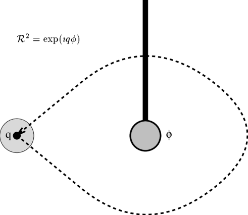
Figure 1.5: Taking a screened external charge $q$ around a magnetic vortex $\phi$ in the Higgs medium generates the Aharonov-Bohm phase $\exp(\imath q\phi)$. We have emphasized the extended structure of these sources, although this structure will not be probed in the low energy regime to which we confine ourselves here. The shaded region around the external point charge $q$ represents the cloud of screening charge of characteristic size $1/M_{A}$. The flux of the vortex is confined to the shaded circle bounded by the core at the distance $1/M_{H}$ from its centre. The string attached to the core represents the Dirac string of the flux, i.e. the strip in which the nontrivial parallel transport in the gauge fields takes place.

Consider the system depicted in figure 1.5 consisting of an external charge $q$ and a magnetic vortex $\phi$ in the Higgs medium well separated from each other. We have depicted these sources as extended objects, but in the low energy regime their extended structure will never be probed and it is legitimate to describe these sources as point particles moving in the plane. The magnetic vortex introduces a nontrivial holonomy (1.3.23) in the gauge fields to which the external charge couples through the matter coupling (1.3.3)

$$-\int\!\!d\,^{2}x\;j^{\kappa}A_{\kappa} = \frac{q\phi}{2\pi}\dot{\chi}_{\phi}({\bf y}(t)-{\bf z}(t)).$$ (1.3.24)

Here, ${\bf y}(t)$ and ${\bf z}(t)$ respectively denote the worldlines of the external charge $q$ and magnetic vortex $\phi$ in the plane. In the conventions we will use throughout these notes, the nontrivial parallel transport in the gauge fields around the magnetic vortices takes place in a thin strip (simply called Dirac string from now) attached to the core of the vortex going off to spatial infinity in the direction of the positive vertical axis. This situation can always be reached by a smooth gauge transformation, and simplifies the bookkeeping for the braid processes involving more than two particles. The multi-valued function $\chi_{\phi}({\bf x})$ with support in the aforementioned strip of parallel transport is a direct translation of this convention. It increases from $0$ to $2\pi$ if the strip is passed from right to left. Thus, when the external charge $q$ moves through this strip once in the counterclockwise fashion indicated in figure 1.5, the topological interaction Lagrangian (1.3.24) generates the action $q\phi$. In the same process the screening charge $q_{\rm scr}=-q$ accompanying the external charge $q$ also moves through this strip of parallel transport. Since the screening charge has a sign opposite to the sign of the external charge, it seems, at first sight, that the total topological action associated with encircling a flux by a screened external charge vanishes. This is not the case though. The screening charge $q_{\rm scr}$ not only couples to the holonomy in the gauge field $A_{\kappa}$ around the vortex but also to the holonomy in the Goldstone boson field $\sigma$. This follows directly from the effective low energy Lagrangian (1.3.11). Let $j_{\rm scr}^{\kappa}$ be the screening current (1.3.16) associated with the screening charge $q_{\rm scr}$. The interaction term in (1.3.11) couples this current to the massive gauge invariant field $\tilde{A}_{\kappa}$ around the vortex: $-j_{\rm scr}^{\kappa}\tilde{A}_{\kappa}$. As we have seen in (1.3.22), the holonomies in the gauge field and the Goldstone boson field are related at large distances from the core of the vortex, such that $\tilde{A}_{\kappa}$ strictly vanishes. As a consequence, the interaction term $-j_{\rm scr}^{\kappa}\tilde{A}_{\kappa}$ vanishes and indeed the matter coupling (1.3.24) summarizes all the remaining long range interactions in the low energy regime [sam].

Being a total time derivative, the topological interaction term (1.3.24) does not appear in the equations of motion and has no effect at the classical level. In the first quantized description, however, the appearance of this term has far reaching consequences. This is most easily seen using the path integral method for quantization. In the path integral formalism, the transition amplitude or propagator from one point in the configuration space at some time to another point at some later time, is given by a weighed sum over all the paths connecting the two points. In this sum, the paths are weighed by their action $\exp(\imath S)$. If we apply this prescription to our charge/flux system, we see that the Lagrangian (1.3.24) assigns amplitudes differing by $\exp(\imath q\phi)$ to paths differing by an encircling of the external charge $q$ around the flux $\phi$. Thus nontrivial interference takes place between paths associated with different winding numbers of the charge around the flux. This is the Aharonov-Bohm effect which becomes observable in quantum interference experiments [ahabo], such as low energy scattering experiments of external charges from the magnetic vortices. The cross sections measured in these Aharonov-Bohm scattering experiments can be found in appendix LABEL:ahboverl.

There are two equivalent ways to present the appearance of the Aharonov-Bohm interactions. In the above discussion of the path integral formalism we kept the topological Aharonov-Bohm interactions in the Lagrangian for this otherwise free charge/flux system. In this description we work with single valued wave functions on the configuration space for a given time slice

$$\Psi_{q\phi}({\bf y},{\bf z},t) = \Psi_{q}({\bf y},t)\Psi_{\phi}({\bf z},t)\qquad\qquad\mbox{with ${\bf y}\neq{\bf z}$}.$$ (1.3.25)

The factorization of the wave functions follows because there are no interactions between the external charge and the magnetic flux other then the topological one (1.3.24). The time evolution of these wave functions is given by the propagator associated with the two particle Lagrangian

$$L = \frac{1}{2}m_{q}\dot{{\bf y}}^{2}+\frac{1}{2}m_{\phi}\dot{{\bf z}}^{2}+\frac{q\phi}{2\pi}\dot{\chi}_{\phi}({\bf y}(t)-{\bf z}(t)).$$ (1.3.26)

Equivalently, we may absorb the topological interaction (1.3.24) in the boundary condition of the wave functions and work with multi-valued wave functions

$$\tilde{\Psi}_{q\phi}({\bf y},{\bf z},t) := e^{\imath\frac{q\phi}{2\pi}\chi_{\phi}({\bf y}-{\bf z})}\;\Psi_{q}({\bf y},t)\Psi_{\phi}({\bf z},t),$$ (1.3.27)

which propagate with a completely free two particle Lagrangian [wu] (see also [forte])

$$\tilde{L} = \frac{1}{2}m_{q}\dot{{\bf y}}^{2}+\frac{1}{2}m_{\phi}\dot{{\bf z}}^{2}.$$ (1.3.28)

We cling to the latter description from now on. That is, we will always absorb the topological interaction terms in the boundary condition of the wave functions. For later use and convenience, we set some more conventions. We will adopt a compact Dirac notation emphasizing the internal charge/flux quantum numbers of the particles. In this notation, the quantum state describing a charge or flux localized at some position ${\bf x}$ in the plane is presented as

$$|{\rm charge/flux}\rangle:=|{\rm charge/flux},{\bf x}\rangle=|{\rm charge/flux}\rangle|{\bf x}\rangle.$$ (1.3.29)

To proceed, the charges $q=ne$ will be abbreviated by the number $n$ of fundamental charge units $e$ and the fluxes $\phi$ by the number $a$ of fundamental flux units $\frac{2\pi}{Ne}$. With the two particle quantum state $|n\rangle|a\rangle$ we then indicate the multi-valued wave function

$$|n\rangle|a\rangle := e^{\imath\frac{na}{N}\chi_{a}({\bf x}-{\bf y})}\;|n,{\bf x}\rangle|a,{\bf y}\rangle,$$ (1.3.30)

where by convention the particle that is located most left in the plane (in this case the external charge $q=ne$), appears most left in the tensor product. The process of transporting the charge adiabatically around the flux in a counterclockwise fashion as depicted in figure 1.5 is now summarized by the action of the monodromy operator on this two particle state

$${\cal R}^{2}\;|n\rangle|a\rangle = e^{\frac{2\pi\imath}{N}na}\;|n\rangle|a\rangle,$$ (1.3.31)

which boils down to a residual global ${\bf Z}_{N}$ transformation by the flux $a$ of the vortex on the charge $n$.

Given the remaining long range Aharonov-Bohm interactions (1.3.31) in the Higgs phase, the labeling of the charges and the fluxes by integers is, of course, highly redundant. Charges $n$ differing by a multiple of $N$ can not be distinguished. The same holds for the fluxes $a$. Hence, the charge and flux quantum numbers are defined modulo $N$ in the residual manifest ${\bf Z}_{N}$ gauge theory describing the long distance physics of the model (1.3.1). Besides these pure ${\bf Z}_{N}$ charges and fluxes the full spectrum naturally consists of charge/flux composites or dyons produced by fusing the charges and fluxes. We return to a detailed discussion of this spectrum and the topological interactions it exhibits in the next section.

Let us recapitulate our results from a more conceptual point of view (see also [alfrev, kli, preskra] in this connection). In unbroken (compact) quantum electrodynamics, the quantized matter charges $q=ne$ (with $n\in{\bf Z}$), corresponding to the different unitary irreducible representations (UIR’s) of the global symmetry group $U(1)$, carry long range Coulomb fields. In other words, the Hilbert space of this theory decomposes into a direct sum of orthogonal charge superselection sectors that can be distinguished by measuring the associated Coulomb fields at spatial infinity. Local observables preserve this decomposition, since they can not affect these long range properties of the charges. The charge sectors can alternatively be distinguished by their response to global $U(1)$ transformations, since these are related to physical measurements of the Coulomb fields at spatial infinity through Gauss’ law. Let us emphasize that the states in the Hilbert space are of course invariant under local gauge transformations, i.e. gauge transformations with finite support, which become trivial at spatial infinity.

Here, we touch upon the important distinction between global symmetry transformations and local gauge transformations. Although both leave the action of the model invariant, their physical meaning is rather different. A global symmetry (independent of the coordinates) is a true symmetry of the theory and in particular leads to a conserved Noether current. Local gauge transformations, on the other hand, correspond to a redundancy in the variables describing a given model and should therefore be modded out in the construction of the physical Hilbert space. In the $U(1)$ gauge theory under consideration the fields that transform nontrivially under the global $U(1)$ symmetry are the matter fields. The associated Noether current $j^{\kappa}$ shows up in the Maxwell equations. More specifically, the conserved Noether charge $q=\int d\,^{2}x\,j^{0}$, being the generator of the global symmetry, is identified with the Coulomb charge $Q=\int d\,^{2}x\,\nabla\cdot{\bf E}$ through Gauss’ law. This is the aforementioned relation between the global symmetry transformations and physical Coulomb charge measurements at spatial infinity.

Although the long range Coulomb fields vanish when this $U(1)$ gauge theory is spontaneously broken down to a finite cyclic group ${\bf Z}_{N}$, we are still able to detect ${\bf Z}_{N}$ charge at arbitrary long distances through the Aharonov-Bohm effect. In other words, there remains a relation between residual global symmetry transformations and physical charge measurements at spatial infinity. The point is that we are left with a gauged ${\bf Z}_{N}$ symmetry in the Higgs phase, as witnessed by the appearance of stable magnetic fluxes in the spectrum. The magnetic fluxes introduce holonomies in the (locally flat) gauge fields, which take values in the residual manifest gauge group ${\bf Z}_{N}$ to leave the Higgs condensate single valued. To be specific, the holonomy of a given flux is classified by the group element picked up by the Wilson loop operator

$$W({\cal C},{\bf x}_{0}) = P\exp\,(\imath e\oint A^{i}dl^{i})\;\in{\bf Z}_{N},$$ (1.3.32)

where ${\cal C}$ denotes a loop enclosing the flux starting and ending at some fixed base point ${\bf x}_{0}$ at spatial infinity. The path ordering indicated by $P$ is trivial in this abelian case. These fluxes can be used for charge measurements in the Higgs phase by means of the Aharonov-Bohm effect (1.3.31). This purely quantum mechanical effect, boiling down to a global ${\bf Z}_{N}$ gauge transformation on the charge by the group element (1.3.32), is topological. It persists at arbitrary long ranges and therefore distinguishes the nontrivial ${\bf Z}_{N}$ charge sectors in the Higgs phase. Thus the result of the Higgs mechanism for the charge sectors can be summarized as follows: the charge superselection sectors of the original $U(1)$ gauge theory, which were in one-to-one correspondence with the UIR’s of the global symmetry group $U(1)$, branch to UIR’s of the residual (gauged) symmetry group ${\bf Z}_{N}$ in the Higgs phase.

An important conclusion from the foregoing discussion is that a spontaneously broken $U(1)$ gauge theory in general can have distinct Higgs phases corresponding to different manifest cyclic gauge groups ${\bf Z}_{N}$. The simplest example is a $U(1)$ gauge theory with two Higgs fields; one carrying a charge $Ne$ and the other a charge $e$. There are in principle two possible Higgs phases in this particular theory, depending on whether the ${\bf Z}_{N}$ gauge symmetry remains manifest or not. In the first case only the Higgs field with charge $Ne$ is condensed and we are left with nontrivial ${\bf Z}_{N}$ charge sectors. In the second case the Higgs field carrying the fundamental charge $e$ is condensed. No charge sectors survive in this completely broken phase. These two Higgs phases, separated by a phase transition, can clearly be distinguished by probing the existence of ${\bf Z}_{N}$ charge sectors. This is exactly the content of the nonlocal order parameter constructed by Preskill and Krauss [preskra] (see also [alflee, alfmarc, alfrev, lo, poli] in this context). In contrast with the Wilson loop operator and the ’t Hooft loop operator distinguishing the Higgs and confining phase of a given gauge theory through the dynamics of electric and magnetic flux tubes [thooft, wilson], this order parameter is of a topological nature. To be specific, in this 2+1 dimensional setting it amounts to evaluating the expectation value of a closed electric flux tube linked with a closed magnetic flux loop corresponding to the worldlines of a minimal ${\bf Z}_{N}$ charge/anti-charge pair linked with the worldlines of a minimal ${\bf Z}_{N}$ magnetic flux/anti-flux pair. If the ${\bf Z}_{N}$ gauge symmetry is manifest, this order parameter gives rise to the Aharonov-Bohm phase (1.3.31), whereas it becomes trivial in the completely broken phase with minimal stable flux $\frac{2\pi}{e}$.

1.3.3 Braid and fusion properties of the spectrum

We proceed with a more thorough discussion of the topological interactions described by the residual ${\bf Z}_{N}$ gauge theory featuring in the Higgs phase of the model (1.3.1). As we have argued in the previous section, the complete spectrum consists of pure ${\bf Z}_{N}$ charges labeled by $n$, pure ${\bf Z}_{N}$ fluxes labeled by $a$ and dyons produced by fusing these charges and fluxes:

$$|a\rangle\times|n\rangle = |a,n\rangle\qquad\qquad\mbox{with}\qquad a,n\in 0,1,\ldots,N-1.$$ (1.3.33)

We have depicted this spectrum for a ${\bf Z}_{4}$ gauge theory in figure 1.6.

Figure 1.6: The spectrum of a Higgs phase featuring a residual manifest gauge group ${\bf Z}_{4}$ compactifies to the particles inside the dashed box. The particles outside the box are identified with the ones inside by means of modulo $4$ calculus along the charge and flux axes. The modulo $4$ calculus for the fluxes corresponds to Dirac monopoles/instantons, if these are present. That is, the minimal monopole tunnels the encircled flux into the vacuum.

The topological interactions described by a ${\bf Z}_{N}$ gauge theory are completely governed by the Aharonov-Bohm effect (1.3.31) and can simply be summarized as follows

$${\cal R}^{2}\;|a,n\rangle|a^{\prime},n^{\prime}\rangle = e^{\frac{2\pi\imath}{N}(na^{\prime}+n^{\prime}a)}\;|a,n\rangle|a^{\prime},n^{\prime}\rangle$$ (1.3.34)

$${\cal R}\;|a,n\rangle|a,n\rangle = e^{\frac{2\pi\imath}{N}na}\;|a,n\rangle|a,n\rangle$$ (1.3.35)

$$|a,n\rangle\times|a^{\prime},n^{\prime}\rangle = |[a+a^{\prime}],[n+n^{\prime}]\rangle$$ (1.3.36)

$${\cal C}\,|a,n\rangle = |[-a],[-n]\rangle$$ (1.3.37)

$$T\,|a,n\rangle = e^{\frac{2\pi\imath}{N}na}\;|a,n\rangle.$$ (1.3.38)

The expressions (1.3.34) and (1.3.35) sum up the braid properties of the particles in the spectrum (1.3.33). These realize abelian representations of the braid groups discussed in section 1.2. Of course, for distinguishable particles only the monodromies, as contained in the pure or colored braid groups are relevant. (See the discussion concerning relation (1.2.7) for the definition of colored braid groups). In the present context, particles carrying different charge and magnetic flux are distinguishable. When a given particle $|a,n\rangle$ located at some position in the plane is adiabatically transported around another remote particle $|a^{\prime},n^{\prime}\rangle$ in the counterclockwise fashion depicted in figure 1.4, the total multi-valued wave function of the system picks up the Aharonov-Bohm phase displayed in (1.3.34). In this process, the charge $n$ of the first particle moves through the Dirac string attached to the flux $a^{\prime}$ of the second particle, while the charge $n^{\prime}$ of the second particle moves through the Dirac string of the flux $a$ of the first particle. In short, the total Aharonov-Bohm effect for this monodromy is the composition of a global ${\bf Z}_{N}$ symmetry transformation on the charge $n$ by the flux $a^{\prime}$ and a global transformation on the charge $n^{\prime}$ by the flux $a$. We confined ourselves to the case of two particles so far. The generalization to systems containing more then two particles is straightforward. The quantum states describing these systems are tensor products of localized single particle states $|a,n,{\bf x}\rangle$, where we cling to the convention that the particle that appears most left in the plane appears most left in the tensor product. These multi-valued wave functions carry abelian representations of the colored braid group: the action of the monodromy operators (1.2.7) on these wave functions boils down to the quantum phase in expression (1.3.34).

For identical particles, i.e. particles carrying the same charge $n$ and flux $a$, the braid operation depicted in figure 1.1 becomes meaningful. In this braid process, in which two adjacent identical particles $|a,n\rangle$ located at different positions in the plane are exchanged in a counterclockwise way, the charge of the particle that moves ‘behind’ the other dyon encounters the Dirac string attached to the flux of the latter. The result of this exchange in the multi-valued wave function is the quantum statistical phase factor (see expression (1.2.5) of section 1.2) presented in (1.3.35). In other words, the dyons in the spectrum of this ${\bf Z}_{N}$ theory are anyons. In fact, these charge/flux composites are very close to Wilczek’s original proposal for anyons [wilcchfl].

An important aspect of this theory is that the particles in the spectrum (1.3.33) satisfy the canonical spin-statistics connection. The proof of this connection is of a topological nature and applies in general to all the models that will be considered in these notes. The fusion rules play a role in this proof and we will discuss these first.

Fusion and braiding are intimately related. Bringing two particles together is essentially a local process. As such, it can never affect global properties of the system. Hence, the single particle state that arises after fusion should exhibit the same global properties as the two particle state we started with. In this topological theory, the global properties of a given configuration are determined by its braid properties with the different particles in the spectrum (1.3.33). In the previous section, we had already established that the charges and fluxes become ${\bf Z}_{N}$ quantum numbers under these braid properties. Therefore, the complete set of fusion rules, determining the way the charges and fluxes of a two particle state compose into the charge and flux of a single particle state when the pair is brought together, can be summarized as (1.3.36). The rectangular brackets denote modulo $N$ calculus such that the sum always lies in the range $0,1,\ldots,N-1$.

It is worthwhile to digress a little on the dynamical mechanism underlying the modulo $N$ calculus compactifying the flux part of the spectrum. This modulo calculus is induced by magnetic monopoles, when these are present. The presence of magnetic monopoles can be accounted for by assuming that the compact $U(1)$ gauge theory (1.3.1) arises from a spontaneously broken $SO(3)$ gauge theory. The monopoles we obtain in this particular model are the regular ’t Hooft-Polyakov monopoles [thooftmon, polyamon]. Let us, alternatively, assume that we have singular Dirac monopoles [dirac] in this compact $U(1)$ gauge theory. In three spatial dimensions, these are point particles carrying magnetic charges $g$ quantized as $\frac{2\pi}{e}$. In the present 2+1 dimensional Minkowski setting, they become instantons describing flux tunneling events $|\Delta\phi|=\frac{2\pi}{e}$. As has been shown by Polyakov [polyakov], the presence of these instantons in unbroken $U(1)$ gauge theory has a striking dynamical effect. It leads to linear confinement of electric charge. In the broken version of these theories, in which we are interested, electric charge is screened and the presence of instantons in the Higgs phase merely implies that the magnetic flux (1.3.23) of the vortices is conserved modulo $N$

instanton: $$a\;\mapsto\;a-N.$$ (1.3.39)

In other words, a flux $N$ moving in the plane (or $N$ minimal fluxes for that matter) can disappear by ending on an instanton. The fact that the instantons tunnel between states that can not be distinguished by the braidings in this theory is nothing but the 2+1 dimensional space time translation of the unobservability of the Dirac string in three spatial dimensions.

We turn to the connection between spin and statistics. There are in principle two approaches to prove this deep relation, both having their own merits. One approach, originally due to Wightman [streater], involves the axioms of local relativistic quantum field theory, and leads to the observation that integral spin fields commute, while half integral spin fields anticommute. The topological approach that we will take here was first proposed by Finkelstein and Rubinstein [fink]. It does not rely upon the heavy framework of local relativistic quantum field theory and among other things applies to the topological defects considered in this thesis. The original formulation of Finkelstein and Rubinstein was in the 3+1 dimensional context, but it naturally extends to 2+1 dimensional space time as we will discuss now [balach, sen]. See also the references [frohma, frogama] for an algebraic approach.

The crucial ingredient in the topological proof of the spin-statistics connection for a given model is the existence of an anti-particle for every particle in the spectrum, such that the pair can annihilate into the vacuum after fusion. Consider the process depicted at the l.h.s. of the equality sign in figure 1.7. It describes the creation of two separate identical particle/anti-particle pairs from the vacuum, a subsequent counterclockwise exchange of the particles of the two pairs and finally annihilation of the pairs. To keep track of the writhing of the particle trajectories we depict them as ribbons with a white- and a dark side. It is easily verified now that the closed ribbon associated with the process just explained can be continuously deformed into the ribbon at the r.h.s., which corresponds to a counterclockwise rotation of the particle over an angle of $2\pi$ around its own centre. In other words, the effect of interchanging two identical particles in a consistent quantum description should be the same as the effect of rotating one particle over an angle of $2\pi$ around its centre. The effect of this rotation in the wave function is the spin factor $\exp(2\pi\imath s)$ with $s$ the spin of the particle, which in contrast with three spatial dimensions may be any real number in two spatial dimensions. Therefore, the result of exchanging the two identical particles necessarily boils down to a quantum statistical phase factor $\exp(\imath\Theta)$ in the wave function being the same as the spin factor

$$\exp(\imath\Theta) = \exp(2\pi\imath s).$$ (1.3.40)

This is the canonical spin-statistics connection. Actually, a further consistency condition can be inferred from this ribbon argument. The writhing in the particle trajectory can be continuously deformed to a writhing with the same orientation in the anti-particle trajectory. Hence, the anti-particle necessarily carries the same spin and statistics as the particle.

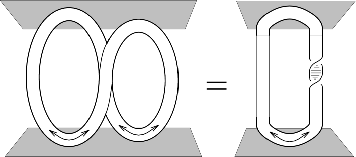
Figure 1.7: Canonical spin-statistics connection. The trajectories describing a counterclockwise interchange of two particles in separate particle/anti-particle pairs (the 8 laying on its back) can be continuously deformed into a single pair in which the particle undergoes a counterclockwise rotation over an angle of $2\pi$ around its own centre (the 0 with a twisted leg).

Sure enough the topological proof of the canonical spin-statistics connection applies to the ${\bf Z}_{N}$ gauge theory at hand. First of all, we can naturally assign an anti-particle to every particle in the spectrum (1.3.33) through the charge conjugation operator (1.3.37). Under charge conjugation the charge and flux of the particles in the spectrum reverse sign and amalgamating a particle with its charge conjugated partner yields the quantum numbers of the vacuum as follows from the fusion rules (1.3.36). Thus the basic assertion for the above ribbon argument is satisfied. From the quantum statistical phase factor (1.3.35) assigned to the particles and (1.3.40), we then conclude that the particles carry spin. Specifically, under rotation over $2\pi$ the single particle states should give rise to the spin factors displayed in (1.3.38). In fact, these spin factors can be interpreted as the Aharonov-Bohm phase generated when the charge of a given dyon rotates around its own flux. Of course, a small separation between the charge and the flux of the dyon is required for this interpretation. Also, note that the particles and their anti-particles indeed carry the same spin and statistics, as follows immediately from the invariance of the Aharonov-Bohm effect under charge conjugation.

Having established a complete classification of the topological interactions described by a ${\bf Z}_{N}$ gauge theory, we conclude with some remarks on the Aharonov-Bohm scattering experiments by which these interactions can be probed. (A concise discussion of these purely quantum mechanical experiments can be found in appendix LABEL:ahboverl of chapter 3). It is the monodromy effect (1.3.34) that is measured in these two particle elastic scattering experiments. To be explicit, the symmetric cross section for scattering a particle $|a,n\rangle$ from a particle $|a^{\prime},n^{\prime}\rangle$ is given by

$$\frac{{\rm d}\sigma}{{\rm d}\theta} = \frac{\sin^{2}\left(\frac{\pi}{N}(na^{\prime}+n^{\prime}a)\right)}{2\pi p\sin^{2}(\theta/2)},$$ (1.3.41)

with $p$ the relative momentum of the two particles and $\theta$ the scattering angle. A subtlety arises in scattering experiments involving two identical particles, however. Quantum statistics enters the scene: exchange processes between the scatterer and the projectile have to be taken into account [anyonbook, preslo]. This leads to the following cross section for Aharonov-Bohm scattering of two identical particles $|a,n\rangle$

$$\frac{{\rm d}\sigma}{{\rm d}\theta} = \frac{\sin^{2}(\frac{2\pi na}{N})}{2\pi p\sin^{2}(\theta/2)}\;+\;\frac{\sin^{2}(\frac{2\pi na}{N})}{2\pi p\cos^{2}(\theta/2)},$$ (1.3.42)

where the second term summarizes the effect of the extra exchange contribution to the direct scattering amplitude.

1.4 Nonabelian discrete gauge theories

The generalization of the foregoing analysis to spontaneously broken models in which we are left with a nonabelian finite gauge group ${H}$ involves some essentially new features. In this introductory section, we will establish the complete flux/charge spectrum of such a nonabelian discrete ${H}$ gauge theory and discuss the basic topological interactions among the different flux/charge composites. The outline is as follows. Section 1.4.1 contains a general discussion on the topological classification of stable magnetic vortices and the subtle role magnetic monopoles play in this classification. In section 1.4.2, we subsequently review the properties of the nonabelian magnetic vortices that occur when the residual symmetry group $H$ is nonabelian. The most important one being that these vortices exhibit a nonabelian Aharonov-Bohm effect. To be specific, the fluxes of the vortices, which are labeled by the group elements of ${H}$, affect each other through conjugation when they move around each other [bais]. Under the residual global symmetry group ${H}$ the magnetic fluxes transform by conjugation as well, and the conclusion is that the vortices are organized in degenerate multiplets, corresponding to the different conjugacy classes of ${H}$. These classical properties will then be elevated into the first quantized description in which the magnetic vortices are treated as point particles moving in the plane. In section 1.4.3, we finally turn to the matter charges that may occur in these Higgs phases and their Aharonov-Bohm interactions with the magnetic vortices. As has been pointed out in [almawil, preskra], these matter charges are labeled by the different UIR’s $\Gamma$ of the residual global symmetry group ${H}$ and when such a charge encircles a nonabelian vortex it picks up a global symmetry transformation by the matrix $\Gamma(h)$ associated with the flux $h$ of the vortex in the representation $\Gamma$. To conclude, we elaborate on the subtleties [spm] involved in the description of dyonic combinations of the nonabelian magnetic fluxes and the matter charges $\Gamma$.

1.4.1 Classification of stable magnetic vortices

Let us start by briefly specifying the spontaneously broken gauge theories in which we are left with a nonabelian discrete gauge theory. In this case, we are dealing with a model governed by a Yang-Mills Higgs action of the form

$$S_{\rm YMH} = \int d\,^{3}x\;(-\frac{1}{4}F^{a\;\kappa\nu}F_{\kappa\nu}^{a}+({\cal D}^{\kappa}\Phi)^{\dagger}\cdot{\cal D}_{\kappa}\Phi-V(\Phi)).$$ (1.4.1)

Here, the Higgs field $\Phi$ transforms according to some higher dimensional representation of a continuous nonabelian gauge group ${G}$, the superscript $a$ naturally labels the generators of the Lie algebra of $G$ and the potential $V(\Phi)$ gives rise to a degenerate set of ground states $\langle\Phi\rangle\neq 0$ which are only invariant under the action of a finite nonabelian subgroup ${H}$ of ${G}$. For simplicity, we make two assumptions. First of all, we assume that this Higgs potential is normalized such that $V(\Phi)\geq 0$ and equals zero for the ground states $\langle\Phi\rangle$. More importantly, we assume that all ground states can be reached from any given one by global ${G}$ transformations. This last assumption implies that the ground state manifold becomes isomorphic to the coset ${G}/{H}$. (Renormalizable examples of potentials doing the job for ${G}\simeq SO(3)$ and ${H}$ some of its point groups can be found in [ovrut]). In the following, we will only be concerned with the low energy regime of this theory, so that the massive gauge bosons can be ignored.

The topologically stable vortices that can be formed in the spontaneously broken gauge theory (1.4.1) correspond to noncontractible maps from the circle at spatial infinity (starting and ending at a fixed base point ${\bf x}_{0}$) into the ground state manifold ${G}/{H}$. Different vortices are related to noncontractible maps that can not be continuously deformed into each other. In short, the different vortices are labeled by the elements of the fundamental group $\pi_{1}$ of ${G}/{H}$ based at the particular ground state $\langle\Phi_{0}\rangle$ the Higgs field takes at the base point ${\bf x}_{0}$ in the plane. (Standard references on the use of homotopy groups in the classification of topological defects are [cola, mermin, presbook, trebin]. See also [poen] for an early discussion on the occurrence of nonabelian fundamental groups in models with a spontaneously broken global symmetry).

The content of the fundamental group $\pi_{1}({G}/{H})$ of the ground state manifold for a specific spontaneously broken model (1.4.1) can be inferred from the exact sequence

$$0\simeq\pi_{1}(H)\rightarrow\pi_{1}(G)\rightarrow\pi_{1}(G/H)\rightarrow\pi_{0}(H)\rightarrow\pi_{0}(G)\simeq 0,$$ (1.4.2)

where the first isomorphism follows from the fact that $H$ is discrete. For convenience, we restrict our considerations to continuous Lie groups $G$ that are path connected, which accounts for the last isomorphism. If $G$ is simply connected as well, i.e. $\pi_{1}({G})\simeq 0$, then the exact sequence (1.4.2) yields the isomorphism

$$\pi_{1}({G}/{H}) \simeq {H},$$ (1.4.3)

where we used the result $\pi_{0}(H)\simeq H$, which holds for finite $H$. Thus, the different magnetic vortices in this case are in one-to-one correspondence with the group elements $h$ of the residual symmetry group ${H}$. When ${G}$ is not simply connected, however, this is not a complete classification. This can be seen by the following simple argument. Let $\bar{G}$ denote the universal covering group of ${G}$ and $\bar{H}$ the corresponding lift of ${H}$ into $\bar{G}$. We then have $G/H=\bar{G}/\bar{H}$ and in particular $\pi_{1}({G}/{H})\simeq\pi_{1}(\bar{G}/\bar{H})$. Since the universal covering group of $G$ is by definition simply connected, that is, $\pi_{1}(\bar{G})\simeq 0$, we obtain the following isomorphism from the exact sequence (1.4.2) for the lifted groups $\bar{G}$ and $\bar{H}$

$$\pi_{1}({G}/{H})\;\simeq\;\pi_{1}(\bar{G}/\bar{H})\;\simeq\;\bar{H}.$$ (1.4.4)

Hence, for a non-simply connected broken gauge group $G$, the different stable magnetic vortices are labeled by the elements of $\bar{H}$ rather then $H$ itself.

It should be emphasized that the extension (1.4.4) of the magnetic vortex spectrum is based on the tacit assumption that there are no Dirac monopoles featuring in this model. In any theory with a non-simply connected gauge group $G$, however, we have the freedom to introduce singular Dirac monopoles ‘by hand’ [later, cola]. The magnetic charges of these monopoles are characterized by the elements of the fundamental group $\pi_{1}(G)$, which is abelian for continuous Lie groups $G$. The exact sequence (1.4.2) for the present spontaneously broken model now implies the identification

$$\pi_{1}(G) \simeq \mbox{Ker}\left(\pi_{1}(G/H)\rightarrow\pi_{0}(H)\right)$$

$$\simeq \mbox{Ker}\left(\bar{H}\rightarrow H\right).$$

In other words, the magnetic charges of the Dirac monopoles are in one-to-one correspondence with the nontrivial elements of $\pi_{1}(G/H)\simeq\bar{H}$ associated with the trivial element in $\pi_{0}(H)\simeq H$. The physical interpretation of this formula is as follows. In the 2+1 dimensional Minkowsky setting, in which we are interested, the Dirac monopoles become instantons describing tunneling events between magnetic vortices $\bar{h}\in\bar{H}$ differing by the elements of $\pi_{1}(G)$. Here, the decay or tunneling time will naturally depend exponentially on the actual mass of the monopoles. The important conclusion is that in the presence of these Dirac monopoles the magnetic fluxes $\bar{h}\in\bar{H}$ are conserved modulo the elements of $\pi_{1}(G)$ and the proper labeling of the stable magnetic vortices boils down to the elements of the residual symmetry group $H$ itself

$$\bar{H}/\pi_{1}(G) \simeq H.$$ (1.4.6)

To proceed, the introduction of Dirac monopoles has a bearing on the matter content of the model as well. The only matter fields allowed in the theory with monopoles are those that transform according to an ordinary representation of $G$. Matter fields carrying a faithful representation of the universal covering group $\bar{G}$ are excluded. This means that the matter charges appearing in the broken phase correspond to ordinary representations of $H$, while faithful representations of the lift $\bar{H}$ do not occur. As a result, the fluxes $\bar{h}\in\bar{H}$ related by tunneling events induced by the Dirac monopoles can not be distinguished through long range Aharonov-Bohm experiments with the available matter charges, which is consistent with the fact that the stable magnetic fluxes are labeled by elements of $H$ rather then $\bar{H}$ in this case.

The whole discussion can now be summarized as follows. First of all, if a simply connected gauge group $G$ is spontaneously broken down to a finite subgroup $H$, we are left with a discrete $H$ gauge theory in the low energy regime. The magnetic fluxes are labeled by the elements of $H$, whereas the different electric charges correspond to the full set of UIR’s of $H$. When we are dealing with a non-simply connected gauge group $G$ broken down to a finite subgroup $H$, there are two possibilities depending on whether we allow for Dirac monopoles/instantons in the theory or not. In case Dirac monopoles are ruled out, we obtain a discrete $\bar{H}$ gauge theory. The stable fluxes are labeled by the elements of $\bar{H}$ and the different charges by the UIR’s of $\bar{H}$. If the model features singular Dirac monopoles, on the other hand, then the stable fluxes simply correspond to the elements of the group $H$ itself, while the allowed matter charges constitute UIR’s of $H$. In other words, we are left with a discrete $H$ gauge theory under these circumstances.

Let us illustrate these general considerations by some explicit examples. First we return to the model discussed in section 1.3, in which the non-simply connected gauge group $G\simeq U(1)$ is spontaneously broken down to the finite cyclic group $H\simeq{\bf Z}_{N}$. The topological classification (1.4.4) for this particular model gives

$$\pi_{1}(U(1)/{\bf Z}_{N})\;\simeq\;\pi_{1}({\bf R}/{\bf Z}_{N}\times{\bf Z})\;\simeq\;{\bf Z}_{N}\times{\bf Z}\;\simeq\;{\bf Z}.$$

Thus, in the absence of Dirac monopoles, the different stable vortices are labeled by the integers in accordance with (1.3.23), where we found that the magnetic fluxes associated with these vortices are quantized as $\phi=\frac{2\pi a}{Ne}$ with $a\in{\bf Z}$. In principle, we are dealing with a discrete ${\bf Z}$ gauge theory now and the complete magnetic flux spectrum could be distinguished by means of long range Aharonov-Bohm experiments with electric charges $q$ being fractions of the fundamental unit $e$, which correspond to the UIR’s of ${\bf Z}$. Of course, this observation is rather academic in this context, since free charges carrying fractions of the fundamental charge unit $e$ have never been observed. With matter charges $q$ being multiples of $e$, the low energy theory then boils down to a ${\bf Z}_{N}$ gauge theory, although the topologically stable magnetic vortices in the broken phase are labeled by the integers $a$. The Dirac monopoles/instantons that can be introduced in this theory correspond to the elements of $\pi_{1}(U(1))\simeq{\bf Z}$. The presence of these monopoles, which carry magnetic charge $g=\frac{2\pi m}{e}$ with $m\in{\bf Z}$, imply that the magnetic flux $a$ of the vortices is conserved modulo $N$, as we have seen explicitly in (1.3.39). In other words, the proper labeling of the stable magnetic fluxes is by the elements of ${\bf Z}_{N}\times{\bf Z}/{\bf Z}\simeq{\bf Z}_{N}$, as indicated by (1.4.6). Moreover, electric charge is necessarily quantized in multiples of the fundamental charge unit $e$ now, so that the tunneling events induced by the instantons are unobservable at long distances. The unavoidable conclusion then becomes that in the presence of Dirac monopoles, we are left with a ${\bf Z}_{N}$ gauge theory in the low energy regime of this spontaneously broken model, in complete accordance with the general discussion of the foregoing paragraphs.

When a gauge theory at some intermediate stage of symmetry breaking exhibits regular ’t Hooft-Polyakov monopoles, their effect on the stable magnetic vortex classification is automatically taken care of, as it should because the monopoles can not be left out in such a theory. Consider, for example, a model in which the non-simply connected gauge group $G\simeq SO(3)$ is initially broken down to $H_{1}\simeq U(1)$ and subsequently to $H_{2}\simeq{\bf Z}_{N}$

$$SO(3)\;\longrightarrow\;U(1)\;\longrightarrow\;{\bf Z}_{N}.$$ (1.4.7)

The first stage of symmetry breaking is accompanied by the appearance of regular ’t Hooft-Polyakov monopoles [thooftmon, polyamon] carrying magnetic charges characterized by the elements of the second homotopy group $\pi_{2}(SO(3)/U(1))\simeq{\bf Z}$. A simple exact sequence argument shows

$$\pi_{2}(SO(3)/U(1)) \simeq \mbox{Ker}\left(\pi_{1}(U(1))\rightarrow\pi_{1}(SO(3))\right)$$

$$\simeq \mbox{Ker}\left({\bf Z}\rightarrow{\bf Z}_{2}\right).$$

Hence, the magnetic charges of the regular monopoles correspond to the elements of $\pi_{1}(U(1))$ associated with the trivial element of $\pi_{1}(SO(3))$, that is, the even elements of $\pi_{1}(U(1))$. In short, the regular monopoles carry magnetic charge $g=\frac{4\pi m}{e}$ with $m\in{\bf Z}$. To proceed, the residual topologically stable magnetic vortices emerging after the second symmetry breaking are labeled by the elements of $\bar{H}_{2}\simeq{\bf Z}_{2N}$, which follows from (1.4.4)

$$\pi_{1}(SO(3)/{\bf Z}_{N})\;\simeq\;\pi_{1}(SU(2)/{\bf Z}_{2N})\;\simeq\;{\bf Z}_{2N}.$$

As in the previous example, the magnetic fluxes carried by these vortices are quantized as $\phi=\frac{2\pi a}{Ne}$, while the presence of the regular ’t Hooft-Polyakov monopoles now causes the fluxes $a$ to be conserved modulo $2N$. The tunneling or decay time will depend on the mass of the regular monopoles, that is, the energy scale associated with the first symmetry breaking in the hierarchy (1.4.7). Here it is assumed that the original $SO(3)$ gauge theory does not feature Dirac monopoles ($g=\frac{2\pi m}{e}$, with $m=0,1$) corresponding to the elements of $\pi_{1}(SO(3))\simeq{\bf Z}_{2}$. This means that additional matter fields carrying faithful (half integral spin) representations of the universal covering group $SU(2)$ are allowed in this model, which leads to half integral charges $q=\frac{ne}{2}$ with $n\in{\bf Z}$ in the $U(1)$ phase. In the final Higgs phase, the half integral charges $q$ and the quantized magnetic fluxes $\phi$ then span the complete spectrum of the associated discrete ${\bf Z}_{2N}$ gauge theory.

Let us now, instead, suppose that the original $SO(3)$ gauge theory contains Dirac monopoles. The complete monopole spectrum arising after the first symmetry breaking in (1.4.7) then consists of the magnetic charges $g=\frac{2\pi m}{e}$ with $m\in{\bf Z}$, which implies that magnetic flux $a$ is conserved modulo $N$ in the final Higgs phase. This observation is in complete agreement with (1.4.6), which states that the proper magnetic flux labeling is by the elements of ${\bf Z}_{2N}/{\bf Z}_{2}\simeq{\bf Z}_{N}$ under these circumstances. In addition, the incorporation of Dirac monopoles rules out matter fields which carry faithful representations of the universal covering group $SU(2)$. Hence, only integral electric charges are conceivable ($q=ne$ with $n\in{\bf Z}$) and all in all we end up with a discrete ${\bf Z}_{N}$ gauge theory in the Higgs phase. This last situation can alternatively be implemented by embedding this spontaneously broken $SO(3)$ gauge theory in an $SU(3)$ gauge theory. In other words, the symmetry breaking hierarchy is extended to

$$SU(3)\;\longrightarrow\;SO(3)\;\longrightarrow\;U(1)\;\longrightarrow\;{\bf Z}_{N}.$$ (1.4.9)

The singular Dirac monopoles in the $SO(3)$ phase then turn into regular ’t Hooft-Polyakov monopoles

$$\pi_{2}(SU(3)/SO(3))\;\simeq\;\pi_{1}(SO(3))\;\simeq\;{\bf Z}_{2}.$$

The unavoidable presence of these monopoles automatically imply that the magnetic flux $a$ of the vortices in the final Higgs phase is conserved modulo $N$. To be specific, a magnetic flux $a=N$ can decay by ending on a regular monopole in this model, where the decay time will again depend on the mass of the monopole or equivalently on the energy scale associated with the first symmetry breaking in (1.4.9). The existence of such a dynamical decay process is implicitly taken care of in the classification (1.4.3), which indicates that the stable magnetic fluxes are indeed labeled by the elements of $\pi_{1}(SU(3)/{\bf Z}_{N})\simeq{\bf Z}_{N}$.

To conclude, in the above examples we restricted ourselves to the case where we are left with an abelian finite gauge group in the Higgs phase. Of course, the discussion extends to nonabelian finite groups as well. The more general picture then becomes as follows. If the non-simply connected gauge group $G\simeq SO(3)$ is spontaneously broken to some (possibly nonabelian) finite subgroup $H\subset SO(3)$, then the topologically stable magnetic fluxes correspond to the elements of the lift $\bar{H}\subset SU(2)\simeq\bar{G}$. In the Higgs phase, we are then left with a discrete $\bar{H}$ gauge theory. If we have embedded $SO(3)$ in $SU(3)$ (or alternatively introduced the conceivable ${\bf Z}_{2}$ Dirac monopoles), on the other hand, then the topologically stable magnetic fluxes correspond to the elements of $H$ itself and we end up with a discrete $H$ gauge theory.

1.4.2 Flux metamorphosis

Henceforth, we assume that the spontaneously broken gauge group $G$ in our model (1.4.1) is simply connected, for convenience. Hence, the stable magnetic vortices are labeled by the elements of the nonabelian residual symmetry group $H$, as indicated by the isomorphism (1.4.3).

We start with a discussion of the classical field configuration associated with a single static nonabelian vortex in the plane. In principle, we are dealing with an extended object with a finite core size proportional to the inverse of the symmetry breaking scale $M_{H}$. In the low energy regime, however, we can neglect this finite core size and we will idealize the vortex as a point singularity in the plane. For finite energy, the associated static classical field configuration then satisfies the equations $V(\Phi)=0$, $F^{\kappa\nu}=0$, ${\cal D}_{i}\Phi=0$ and $A_{0}=0$ outside the core. These equations imply that the Higgs field takes ground state values $\langle\Phi\rangle$ and the Lie algebra valued vector potential $A_{\kappa}$ is pure gauge so that all nontrivial curvature $F^{\kappa\nu}$ is localized inside the core. To be explicit, a path (and gauge) dependent solution w.r.t.  an arbitrary but fixed ground state $\langle\Phi_{0}\rangle$ at an arbitrary but fixed base point ${\bf x}_{0}$ can be presented as

$$\langle\Phi(\bf x)\rangle = W({\bf x},{\bf x}_{0},\gamma)\langle\Phi_{0}\rangle,$$ (1.4.10)

where the untraced path ordered Wilson line integral

$$W({\bf x},{\bf x}_{0},\gamma) = P\exp(\imath e\int_{{\bf x}_{0}}^{\bf x}A^{i}dl^{i}),$$ (1.4.11)

is evaluated along an oriented path $\gamma$ (avoiding the singularity where the vortex is located) from the base point to some other point ${\bf x}$ in the plane. Here, we merely used the fact that the relation ${\cal D}_{i}\langle\Phi\rangle=0$ identifies the parallel transport in the Goldstone boson fields with that in the gauge fields, as we have argued in full detail for the abelian case in section 1.3.2. Now in order to keep the Higgs field single valued, the magnetic flux of the vortex, picked up by the Wilson line integral along a counterclockwise closed loop ${\cal C}$, which starts and ends at the base point and encloses the core, necessarily takes values in the subgroup ${H}_{0}$ of ${G}$ that leaves the ground state $\langle\Phi_{0}\rangle$ at the base point invariant, i.e.

$$W({\cal C},{\bf x}_{0}) = P\exp(\imath e\oint A^{i}dl^{i})\;=\;h\in{H}_{0}.$$ (1.4.12)

The untraced Wilson loop operator (1.4.12) completely classifies the long range properties of the vortex solution. It is invariant under a continuous deformation of the loop ${\cal C}$ that keeps the base point fixed and avoids the core of the vortex. Moreover, it is invariant under continuous gauge transformations that leave the ground state $\langle\Phi_{0}\rangle$ at the base point invariant. As in the abelian case, we fix this residual gauge freedom by sending all nontrivial parallel transport into a narrow wedge or Dirac string from the core of the vortex to spatial infinity as depicted in figure 1.8. It should be emphasized that our gauge fixing procedure for these vortex solutions involves two physically irrelevant choices. First of all, we have chosen a fixed ground state $\langle\Phi_{0}\rangle$ at the base point ${\bf x}_{0}$. This choice merely determines the embedding of the residual symmetry group in ${G}$ to be the stability group ${H}_{0}$ of $\langle\Phi_{0}\rangle$. A different choice for this ground state gives rise to a different embedding of the residual symmetry group, but will eventually lead to an unitarily equivalent quantum description of the discrete ${H}$ gauge theory in the Higgs phase. For convenience, we subsequently fix the remaining gauge freedom by sending all nontrivial transport around the vortices to a small wedge. Of course, physical phenomena will not depend on this choice. In fact, an equivalent formulation of the low energy theory, without fixing this residual gauge freedom for the vortices, can also be given, see for example [bucher].

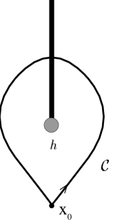
Figure 1.8: Single vortex solution. We have fixed the gauge freedom by sending all nontrivial parallel transport around the core in the Dirac string attached to the core. Thus, outside the core, the Higgs field takes the same ground state value $\langle\Phi_{0}\rangle$ everywhere except for the region where the Dirac string is localized. Here it makes a noncontractible winding in the ground state manifold. This winding corresponds to a holonomy in the gauge field classified by the result of the untraced Wilson loop operator $W({\cal C},{\bf x}_{0})=h\in{H}_{0}$, which picks up the nonabelian magnetic flux located inside the core.

In the gauge fixed prescription described above, we are still able to perform global symmetry transformations $g\in{H}_{0}$ on the vortex solutions that leave the ground state $\langle\Phi_{0}\rangle$ invariant. These transformations affect the field configuration of the vortex in the following way

$$\Phi({\bf x}) \longmapsto g\;\Phi({\bf x})$$ (1.4.13)

$$A_{\kappa}({\bf x}) \longmapsto g\;A_{\kappa}({\bf x})\;g^{-1}.$$ (1.4.14)

As an immediate consequence, we then obtain

$$W({\cal C},{\bf x}_{0}) \longmapsto g\;W({\cal C},{\bf x}_{0})\;g^{-1},$$ (1.4.15)

which shows that the flux of the vortex becomes conjugated $h\mapsto ghg^{-1}$ under a residual global symmetry transformation $g\in{H}_{0}$. The conclusion is that the nonabelian vortex solutions are in fact organized in degenerate multiplets under the residual global symmetry transformations ${H}_{0}$, namely the different conjugacy classes of ${H}_{0}$ denoted as ${}^{A}C$, where $A$ labels a particular conjugacy class. For convenience, we will refer to the stability group of $\langle\Phi_{0}\rangle$ as ${H}$ from now on.

The different vortex solutions in a given conjugacy class ${}^{A}C$ of ${H}$, being related by internal global symmetry transformations that leave the action (1.4.1) invariant, clearly carry the same external quantum numbers, that is, the total energy of the configuration, the coresize etc. These solutions only differ by their internal magnetic flux quantum number. This internal degeneracy becomes relevant in adiabatic interchange processes of remote vortices in the plane. Consider, for instance, the configuration of two remote vortices as presented in figure 1.9. In the depicted adiabatic counterclockwise interchange of these vortices, the vortex initially carrying the magnetic flux $h_{2}$ moves through the Dirac string attached to the other vortex. As a result, its flux picks up a global symmetry transformation by the flux $h_{1}$ of the latter, i.e. $h_{2}\mapsto h_{1}h_{2}h^{-1}_{1}$, such that the total flux of the configuration is conserved. This classical nonabelian Aharonov-Bohm effect appearing for noncommuting fluxes, which has been called flux metamorphosis [bais], leads to physical observable phenomena. Suppose, for example, that the magnetic flux $h_{2}$ was a member of a flux/anti-flux pair $(h_{2},h_{2}^{-1})$ created from the vacuum. When $h_{2}$ encircles $h_{1}$, it returns as the flux $h_{1}h_{2}h^{-1}_{1}$ and will not be able to annihilate the flux $h_{2}^{-1}$ anymore. Upon rejoining the pair we now obtain the stable flux $h_{1}h_{2}h^{-1}_{1}h_{2}$. Moreover, at the quantum level, flux metamorphosis leads to nontrivial Aharonov-Bohm scattering between nonabelian vortices as we will argue in more detail later on.

Residual global symmetry transformations naturally leave the aforementioned observable Aharonov-Bohm effect for nonabelian vortices invariant. This simply follows from the fact that these transformations commute with this nonabelian Aharonov-Bohm effect. To be precise, a residual global symmetry transformation $g\in{H}$ on the two vortex configuration in figure 1.9, for example, affects the flux of both vortices through conjugation by the group element $g$, and it is easily verified that it makes no difference whether such a transformation is performed before the interchange is started or after the interchange is completed. The extension of these classical considerations to configurations of more then two vortices in the plane is straightforward. Braid processes, in which the fluxes of the vortices affect each other by conjugation, conserve the total flux of the configuration. The residual global symmetry transformations $g\in{H}$ of the low energy regime, which act by an overall conjugation of the fluxes of the vortices in the configuration by $g$, commute with these braid processes.

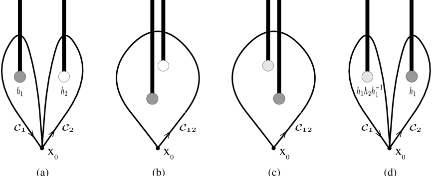
Figure 1.9: Flux metamorphosis. We start off with a classical configuration of two patched vortex solutions, as visualized in figure (a). The vortices are initially assumed to carry the fluxes $W({\cal C}_{1},{\bf x}_{0})=h_{1}$ and $W({\cal C}_{2},{\bf x}_{0})=h_{2}$. The total flux of this configuration is picked up by the Wilson line integral along the loop ${\cal C}_{12}$ encircling both vortices as depicted in figure (b): $W({\cal C}_{12},{\bf x}_{0})=W({\cal C}_{1}\circ{\cal C}_{2},{\bf x}_{0})=W({\cal C}_{1},{\bf x}_{0})\cdot W({\cal C}_{2},{\bf x}_{0})=h_{1}h_{2}$. Now suppose that the two vortices are interchanged in the counterclockwise fashion depicted in figures (b)–(d). In this process vortex 2 moves through the Dirac string attached to vortex 1 and as a result its flux will be affected $h_{2}\mapsto h_{2}^{\prime}$. Vortex 1, on the other hand, never meets any nontrivial parallel transport in the gauge fields and its flux remains the same. Since this local braid process should not be able to change the global properties of this system, i.e. the total flux, we have $h_{1}h_{2}=W({\cal C}_{12},{\bf x}_{0})=W({\cal C}_{1},{\bf x}_{0})\cdot W({\cal C}_{2},{\bf x}_{0})=h_{2}^{\prime}h_{1}$. Thus the flux of vortex 2 becomes conjugated $h_{2}^{\prime}=h_{1}h_{2}h^{-1}_{1}$ by the flux of vortex 1 in this braid process.

As in the abelian case discussed in the previous sections, we wish to treat these nonabelian vortices as point particles in the first quantized description. The degeneracy of these vortices under the residual global symmetry group ${H}$ then indicates that we have to assign a finite dimensional internal Hilbert space $V^{A}$ to these particles, which is spanned by the different fluxes in a given conjugacy class ${}^{A}C$ of ${H}$ and endowed with the standard inner product [spm]

$$\langle h^{\prime}|h\rangle = \delta_{h^{\prime},h}\qquad\qquad\forall\,h,h^{\prime}\in\,^{A}C.$$ (1.4.16)

Under the residual global symmetry transformations the flux eigenstates in this internal Hilbert space $V^{A}$ are affected through conjugation

$$g\in{H}:\qquad|h\rangle \longmapsto |ghg^{-1}\rangle.$$ (1.4.17)

In general, the particle can be in a normalized linear combination of the different flux eigenstates in the internal Hilbert space $V^{A}$. The residual global symmetry transformations (1.4.17) act linearly on such states. Of course, the conjugated action of the residual symmetry group is in general reducible and, at first sight, it seems that we have to decompose this internal Hilbert space into the different irreducible components. This is not the case as we will see in more detail later on (see the discussion concerning relation (1.4.25)). The point is that we can independently perform physical flux measurements by means of quantum interference experiments with electric charges. These measurements project out a particular flux eigenstate. Clearly, these flux measurements do not commute with the residual global symmetry transformations and under their combined action the internal Hilbert spaces $V^{A}$ associated with the different conjugacy classes ${}^{A}C$ form irreducible representations.

The complete quantum state of these particles consists of an internal flux part and an external part. The quantum state describing a single particle in the flux eigenstate $|h_{1}\rangle\in V^{A_{1}}$ at a fixed position ${\bf y}$ in the plane, for instance, is the formal tensor product $|h_{1},{\bf y}\rangle=|h_{1}\rangle|{\bf y}\rangle$. To proceed, the initial configuration depicted in figure 1.9 is described by the multi-valued two particle quantum state $|h_{1},{\bf y}\rangle|h_{2},{\bf z}\rangle$, where again by convention the particle located most left in the plane appears most left in the tensor product. The result of an adiabatic counterclockwise interchange of the two particles can now be summarized by the action of the braid operator

$${\cal R}\;|h_{1},{\bf y}\rangle|h_{2},{\bf z}\rangle = |h_{1}h_{2}h^{-1}_{1},{\bf y}\rangle|h_{1},{\bf z}\rangle,$$ (1.4.18)

which acts linearly on linear combinations of these flux eigenstates. What we usually measure in quantum interference experiments, however, is the effect in the internal wave function of a monodromy of the two particles

$${\cal R}^{2}\;|h_{1},{\bf y}\rangle|h_{2},{\bf z}\rangle = |(h_{1}h_{2})h_{1}(h_{1}h_{2})^{-1},{\bf y}\rangle|h_{1}h_{2}h^{-1}_{1},{\bf z}\rangle.$$ (1.4.19)

This nonabelian Aharonov-Bohm effect can be probed either through a double slit experiment [colem, preslo] or through an Aharonov-Bohm scattering experiment as discussed in appendix LABEL:ahboverl of chapter 3. In the first case, we keep one particle fixed between the two slits, whereas the other particle comes in as a plane wave. The geometry of the Aharonov-Bohm scattering experiment, depicted in figure LABEL:abverpres of appendix LABEL:ahboverl is more or less similar. The interference pattern in both experiments is determined by the internal transition amplitude

$$\langle u_{2}|\langle u_{1}|\;{\cal R}^{2}\;|u_{1}\rangle|u_{2}\rangle,$$ (1.4.20)

where $|u_{1}\rangle$ and $|u_{2}\rangle$ respectively denote the properly normalized internal flux states of the two particles, which are generally linear combinations of the flux eigenstates in the corresponding internal Hilbert spaces $V^{A_{1}}$ and $V^{A_{2}}$. The topological interference amplitudes (1.4.20) summarize all the physical observables for vortex configurations in the low energy regime to which we confine ourselves here. As we have argued before, the residual global symmetry transformations affect internal multi-vortex states through an overall conjugation

$$g\in{H}:\qquad|h_{1}\rangle|h_{2}\rangle \longmapsto |gh_{1}g^{-1}\rangle|gh_{2}g^{-1}\rangle,$$ (1.4.21)

which commutes with the braid operator and therefore leave the interference amplitudes (1.4.20) invariant.

1.4.3 Including matter

Let us now suppose that the total model is of the actual form

$$S = S_{\rm YMH}+S_{\rm matter},$$ (1.4.22)

where $S_{\rm YMH}$ denotes the action for the nonabelian Higgs model given in (1.4.1) and the action $S_{\rm matter}$ describes additional matter fields minimally coupled to the gauge fields. In principle, these matter fields correspond to multiplets which transform irreducibly under the spontaneously broken symmetry group ${G}$. Under the residual symmetry group ${H}$ in the Higgs phase, however, these representations will become reducible and branch to UIR’s $\Gamma$ of ${H}$. Henceforth, it is assumed that the matter content of the model is such that all UIR’s $\Gamma$ of ${H}$ are indeed realized. We will treat the different charges $\Gamma$, appearing in the Higgs phase in this way [almawil, preskra], as point particles. In the first quantized description, these point charges then carry an internal Hilbert space, namely the representation space associated with $\Gamma$. Let us now consider a configuration of a nonabelian vortex in a flux eigenstate $|h\rangle$ at some fixed position in the plane and a remote charge $\Gamma$ in a normalized internal charge state $|v\rangle$ fixed at another position. When the charge encircles the vortex in a counterclockwise fashion, it meets the Dirac string and picks up a global symmetry transformation by the flux of the vortex

$${\cal R}^{2}\;|h,{\bf y}\rangle|v,{\bf z}\rangle = |h,{\bf y}\rangle|\Gamma(h)\,v,{\bf z}\rangle.$$ (1.4.23)

Here, $\Gamma(h)$ is the matrix assigned to the group element $h$ in the representation $\Gamma$. Note, that this Aharonov-Bohm effect boils down to the abelian one given in (1.3.31) in case the residual gauge group $H\simeq{\bf Z}_{N}$. Further, the residual global symmetry transformations on the two particle configuration

$$g\in{H}:\qquad|h,{\bf y}\rangle|v,{\bf z}\rangle \longmapsto |ghg^{-1},{\bf y}\rangle|\Gamma(g)\,v,{\bf z}\rangle,$$ (1.4.24)

again commutes with the monodromy operation (1.4.23). Thus, the interference amplitudes

$$\langle v|\langle h|\;{\cal R}^{2}\;|h\rangle|v\rangle = \langle h|h\rangle\langle v|\Gamma(h)\,v\rangle\;=\;\langle v|\Gamma(h)\,v\rangle,$$ (1.4.25)

measured in either double slit or Aharonov-Bohm scattering experiments involving these particles are invariant under the residual global symmetry transformations. As alluded to before, these interference experiments can be used to measure the flux of a given vortex [colem, alfrev, vohgs, preslo]. To that end, we place the vortex between the two slits (or alternatively use it as the scatterer in an Aharonov-Bohm scattering experiment) and evaluate the interference pattern for an incident beam of charges $\Gamma$ in the same internal state $|v\rangle$. In this way, we determine the interference amplitude (1.4.25). Upon repeating this experiment a couple of times with different internal states for the incident charge $\Gamma$, we can determine all matrix elements of $\Gamma(h)$ and hence, iff $\Gamma$ corresponds to a faithful UIR of ${H}$, the group element $h$ itself. In a similar fashion, we may determine the charge $\Gamma$ of a given particle and, moreover, its internal quantum state $|v\rangle$. In this case, we put the unknown charge between the double slit (or use it as the scatterer in an Aharonov-Bohm scattering experiment), measure the interference pattern for an incident beam of vortices in the same flux eigenstate $|h\rangle$ and again repeat this experiment for all $h\in{H}$.

At this point, we have established the purely magnetic flux and the purely electric charge superselection sectors of the discrete $H$ gauge theory describing the long distance physics of the model (1.4.22). The different magnetic sectors are labeled by the conjugacy classes ${}^{A}C$ of the residual gauge group ${H}$, whereas the different electric charge sectors correspond to the different UIR’s $\Gamma$ of $H$. The complete spectrum of this discrete gauge theory also contains dyonic combinations of these sectors. The relevant remark in this context is that we have not yet completely exhausted the action of the residual global symmetry transformations on the internal magnetic flux quantum numbers. As we have seen in (1.4.17), the residual global ${H}$ transformations affect the magnetic fluxes through conjugation. The transformations that slip through this conjugation may in principle be implemented on an additional internal charge degree of freedom assigned to these fluxes [spm]. More specifically, the global symmetry transformations that leave a given flux $|h\rangle$ invariant are those that commute with this flux, i.e. the group elements in the centralizer ${}^{h}N\subset{H}$. The internal charges that we can assign to this flux correspond to the different UIR’s $\alpha$ of the group ${}^{h}N$. Hence, the inequivalent dyons that can be formed in the composition of a global ${H}$ charge $\Gamma$ with a magnetic flux $|h\rangle$ correspond to the different irreducible components of the subgroup ${}^{h}N$ of ${H}$ contained in the representation $\Gamma$. Two remarks are pertinent now. First of all, the centralizers of different fluxes in a given conjugacy class ${}^{A}C$ are isomorphic. Secondly, the full set of the residual global ${H}$ symmetry transformations relate the fluxes in a given conjugacy class carrying unitary equivalent centralizer charge representations. In other words, the different dyonic sectors are labeled by $(\,^{A}\!C,\alpha\,)$, where ${}^{A}\!C$ runs over the different conjugacy classes of ${H}$ and $\alpha$ over the different nontrivial UIR’s of the associated centralizer. The explicit transformation properties of these dyons under the full global symmetry group ${H}$ involve some conventions, which will be discussed in in the next chapter, where we will identify the Hopf algebra related to a discrete $H$ gauge theory.

The physical observation behind the formal construction of the dyonic sectors [spm] described above, is that we can, in fact, only measure the transformation properties of the charge of a given flux/charge composite under the centralizer of the flux of this composite, see also [preslo]. A similar phenomenon occurs in the 3+1 dimensional setting for monopoles carrying a nonabelian magnetic charge, where it is known as the global color problem [balglob, nelson, nelsonc]. To illustrate this phenomenon, we suppose that we have a composite of a pure flux $|h\rangle$ and a pure global ${H}$ charge $\Gamma$ in some internal state $|v\rangle$. Thus, the complete internal state of the composite becomes $|h,v\rangle$. As we have argued before, the charge of a given object can be determined through double slit or Aharonov-Bohm scattering experiments involving beams of vortices in the same internal flux state $|h^{\prime}\rangle$ and repeating these experiments for all $h^{\prime}\in{H}$. The interference amplitudes measured in this particular case are of the form

$$\langle h,v|\langle h^{\prime}|\;{\cal R}^{2}\;|h^{\prime}\rangle|h,v\rangle = \langle h,v|h^{\prime}hh^{\prime-1},\Gamma(h^{\prime})\,v\rangle\langle h^{\prime}|(h^{\prime}h)h^{\prime}(h^{\prime}h)^{-1}\rangle$$

$$= \langle v|\Gamma(h^{\prime})\,v\rangle\>\delta_{h,h^{\prime}hh^{\prime-1}}\;,$$

where we used (1.4.19) and (1.4.23). As a result of the flux metamorphosis (1.4.19), the interference term is only nonzero for experiments involving fluxes $h^{\prime}$ that commute with the flux of the composite, i.e. $h^{\prime}\in$$\,{}^{h}N$. Hence, we are only able to detect the response of the charge $\Gamma$ of the composite to global symmetry transformations in ${}^{h}N$. This topological obstruction is usually summarized with the statement [alice, balglob2, preskra, schwarz] that in the background of a single vortex $h$, the only ‘realizable’ global symmetry transformations are those taking values in the centralizer ${}^{h}N$.

Let us close this section with a summary of the main conclusions. First of all, the complete spectrum of the nonabelian discrete ${H}$ gauge theory describing the long distance physics of the spontaneously broken model (1.4.22) can be presented as

$$(\,^{A}\!C,\alpha\,),$$ (1.4.27)

where ${}^{A}\!C$ runs over the conjugacy classes of ${H}$ and $\alpha$ denotes the different UIR’s of the centralizer associated to a specific conjugacy class ${}^{A}\!C$. The purely magnetic sectors correspond to trivial centralizer representations and are labeled by the different nontrivial conjugacy classes. The pure charge sectors, on the other hand, correspond to the trivial conjugacy class (with centralizer the full group ${H}$) and are labeled by the different nontrivial UIR’s of the residual symmetry group ${H}$. The other sectors describe the dyons in this theory. Note that the sectors (1.4.27) boil down to the sectors of the spectrum (1.3.33) in case ${H}\simeq{\bf Z}_{N}$.

The residual long range interactions between the particles in the spectrum (1.4.27) of a discrete $H$ gauge theory are topological Aharonov-Bohm interactions. In a counterclockwise braid process involving two given particles, the internal quantum state of the particle that moves through the Dirac string attached to the flux of the other particle picks up a global symmetry transformation by this flux. This (in general nonabelian) Aharonov-Bohm effect conserves the total flux of the system and moreover commutes with the residual global ${H}$ transformations, which act simultaneously on the internal quantum states of all the particles in the system. The last property ensures that the physical observables for a given system, which are all related to this Aharonov-Bohm effect, are invariant under global ${H}$ transformations.

An exhaustive treatment of the spin, braid and fusion properties of the particles in the spectrum (1.4.27) of a (nonabelian) discrete $H$ gauge theory involves the Hopf algebra $D(H)$ related to a discrete ${H}$ gauge theory, which will be discussed in the next chapter. For notational simplicity, we will omit explicit mentioning of the external degrees of freedom of the particles in the following. In our considerations, we usually work with position eigenstates for the particles unless we are discussing double slit- or Aharonov-Bohm scattering experiments in which the incoming projectiles are in momentum eigenstates.

Chapter 2 Algebraic structure

It is by now well-established that there are deep connections between two dimensional rational conformal field theory, three dimensional topological field theory and quantum groups or Hopf algebras. See for instance [alvarez1, alvarez2, witten] and references therein. Discrete $H$ gauge theories, being examples of three dimensional topological field theories, naturally fit in this general scheme. As has been argued in [spm], see also the references [spm1, sm], the algebraic structure related to a discrete $H$ gauge theory is the quasitriangular Hopf algebra $D(H)$ being the result of applying Drinfeld’s quantum double construction [drin, drinfeld] to the abelian algebra ${\cal F}(H)$ of functions on the finite group ${H}$.  Considered as a vector space, we then have $D(H)={\cal F}(H)\otimes{\bf C}[H]$, where ${\bf C}[H]$ denotes the group algebra over the complex numbers ${\bf C}$. Loosely speaking, the elements spanning the Hopf algebra $D(H)$ signal the flux of the particles (1.4.27) in the spectrum of the related discrete $H$ gauge theory and implement the residual global symmetry transformations. Under this action the particles form irreducible representations. Moreover, the algebra $D({H})$ provides an unified description of the spin, braid and fusion properties of the particles. Henceforth, we will simply refer to the algebra $D({H})$ as the quantum double. This name, inspired by its mathematical construction, also summarizes nicely the physical content of a Higgs phase with a residual finite gauge group $H$. The topological interactions between the particles are of a quantum mechanical nature, whereas the spectrum (1.4.27) exhibits an electric/magnetic self-dual (or double) structure.

In fact, the quantum double $D({H})$ was first proposed by Dijkgraaf, Pasquier and Roche [dpr]. They identified it as the Hopf algebra associated with certain holomorphic orbifolds of rational conformal field theories [dvvv] and the related three dimensional topological field theories with finite gauge group $H$ as introduced by Dijkgraaf and Witten [diwi]. The new insight that emerged in [spm, spm1, sm] was that such a topological field theory finds a natural realization as the residual discrete $H$ gauge theory describing the long range physics of gauge theories in which some continuous gauge group $G$ is spontaneously broken down to a finite subgroup $H$.

Here, we review the notion of the quantum double $D(H)$ and elaborate on the unified description this framework gives of the spin, braid and fusion properties of the topological and ordinary particles in the spectrum of a discrete $H$ gauge theory.

2.1 Quantum double

As has been argued in section 1.4.3, we are basically left with two physical operations on the particles (1.4.27) in the spectrum of a discrete ${H}$ gauge theory. We can independently measure their magnetic flux and their electric charge through quantum interference experiments. The magnetic flux of a particle is given by a group element $h\in{H}$, while the charge forms an unitary irreducible representation of the centralizer ${}^{h}N$ of the flux $h\in{H}$ carried by the particle. Flux measurements then correspond to operators ${\rm P}_{h}$ projecting out a particular flux $h$, while the charge of a given particle can be detected through its transformation properties under the residual global symmetry transformations $g\in^{h}N\subset H$ that commute with the flux $h$ of the particle.

The operators ${\rm P}_{h}$ projecting out the flux $h\in{H}$ of a given quantum state naturally realize the projector algebra

$${\rm P}_{h}{\rm P}_{h^{\prime}} = \delta_{h,h^{\prime}}\;{\rm P}_{h},$$ (2.1.1)

with $\delta_{h,h^{\prime}}$ the kronecker delta function for the group elements $h,h^{\prime}\in{H}$. As we have seen in relation (1.4.17), global symmetry transformations $g\in{H}$ affect the fluxes through conjugation. This implies that the flux projection operators and global symmetry transformations for a nonabelian finite gauge group $H$ do not commute

$$g\,{\rm P}_{h} = {\rm P}_{ghg^{-1}}\,g.$$ (2.1.2)

The combination of global symmetry transformations followed by flux measurements

$$\{{\rm P}_{h}\,g\}_{h,g\in{H}},$$ (2.1.3)

generate the quantum double $D({H})={\cal F}(H)\otimes{\bf C}[H]$ and the multiplication (2.1.1) and (2.1.2) of these elements can be recapitulated as 

$${\rm P}_{h}\,g\cdot{\rm P}_{h^{\prime}}\,g^{\prime} = \delta_{h,gh^{\prime}g^{-1}}\;{\rm P}_{h}\,gg^{\prime}.$$ (2.1.4)

The different particles (1.4.27) in the spectrum of the associated discrete ${H}$ gauge theory constitute the complete set of inequivalent irreducible representations of the quantum double $D({H})$. To make explicit the irreducible action of the quantum double on these particles, we have to develop some further notation. To start with, we will label the group elements in the different conjugacy classes of ${H}$ as

$${}^{A}\!C = \{^{A}\!h_{1},\;^{A}\!h_{2},\ldots,\,^{A}\!h_{k}\}.$$ (2.1.5)

Let ${}^{A}\!N\subset{H}$ be the centralizer of the group element ${}^{A}\!h_{1}$ and $\{^{A}\!x_{1},\,^{A}\!x_{2},\ldots,\,^{A}\!x_{k}\}$ a set of representatives for the equivalence classes of ${H}/^{A}\!N$, such that ${}^{A}\!h_{i}=\,^{A}\!x_{i}\,^{A}\!h_{1}\,^{A}\!x_{i}^{-1}$. For convenience, we will always take ${}^{A}\!x_{1}=e$, with $e$ the unit element in ${H}$. To proceed, the basis vectors of the unitary irreducible representation ${\alpha}$ of the centralizer ${}^{A}\!N$ will be denoted by ${}^{\alpha}\!v_{j}$. With these conventions, the internal Hilbert space $V^{A}_{\alpha}$ is spanned by the quantum states

$$\{|\,^{A}\!h_{i},\,^{\alpha}\!v_{j}\rangle\}_{i=1,\ldots,k}^{j=1,\ldots,\mbox{\scriptsize dim}{\,\alpha}}.$$ (2.1.6)

The combined action of a global symmetry transformation $g\in{H}$ followed by a flux projection operation ${\rm P}_{h}$ on these internal flux/charge eigenstates spanning the Hilbert space $V^{A}_{\alpha}$ can then be presented as [dpr]

$$\Pi^{A}_{\alpha}(\,{\rm P}_{h}\,{g}\,)\;|\,^{A}\!h_{i},\,^{\alpha}\!v_{j}\rangle = \delta_{h,g\,^{A}\!h_{i}\,g^{-1}}\;\;|\,g\,^{A}\!h_{i}\,g^{-1},\,{\alpha}(\tilde{g})_{mj}\,^{\alpha}v_{m}\rangle,$$ (2.1.7)

with

$$\tilde{g} := \,{}^{A}\!x_{k}^{-1}\,g\,\,^{A}\!x_{i},$$ (2.1.8)

and $\,{}^{A}\!x_{k}$ defined through $\,{}^{A}\!h_{k}:=g\,^{A}\!h_{i}\,g^{-1}$. It is easily verified that this element $\tilde{g}$ constructed from $g$ and the flux ${}^{A}\!h_{i}$ indeed commutes with ${}^{A}\!h_{1}$ and therefore can be implemented on the centralizer charge. Two remarks are pertinent now. First of all, there is of course arbitrariness involved in the ordering of the elements in the conjugacy classes and the choice of the representatives $\,{}^{A}\!x_{k}$ for the equivalence classes of the coset ${H}/^{A}\!N$. However, different choices lead to unitarily equivalent representations of the quantum double. Secondly, note that (2.1.7) is exactly the action anticipated in section 1.4. The flux ${}^{A}\!h_{i}$ of the associated particle is conjugated by the global symmetry transformation $g\in{H}$, while the part of $g$ that slips through this conjugation is implemented on the centralizer charge of the particle. The operator ${\rm P}_{h}$ subsequently projects out the flux $h$.

We will now argue that the flux/charge eigenstates (2.1.6) spanning the internal Hilbert space $V^{A}_{\alpha}$ carry the same spin, i.e. a counterclockwise rotation over an angle of $2\pi$ gives rise to the same spin factor for all quantum states in $V^{A}_{\alpha}$. As in our discussion of the (abelian) ${\bf Z}_{N}$ gauge theory in section 1.3.3, we assume a small seperation between the centralizer charge and the flux of the particles. In the aforementioned rotation, the centralizer charge of the particle then moves through the Dirac string attached to its flux and as a result picks up a transformation by this flux. The element in the quantum double that implements this effect on the internal quantum states (2.1.6) is the central element

$$\sum_{h}\;{\rm P}_{h}\,h.$$ (2.1.9)

It signals the flux of the internal quantum state and implements this flux on the centralizer charge

$$\Pi^{A}_{\alpha}(\,\sum_{h}\;{\rm P}_{h}\,h\,)\;|\,^{A}\!h_{i},\,^{\alpha}\!v_{j}\rangle = |\,^{A}\!h_{i},\,{\alpha}(^{A}\!h_{1})_{mj}\,^{\alpha}v_{m}\rangle,$$ (2.1.10)

which boils down to the same matrix ${\alpha}(^{A}\!h_{1})$ for all fluxes ${}^{A}\!h_{i}$ in ${}^{A}\!C$. Here, we used (2.1.7) and (2.1.8). Since ${}^{A}\!h_{1}$ by definition commutes with all the elements in the centralizer ${}^{A}\!N$, it follows from Schur’s lemma that it is proportional to the unit matrix in the irreducible representation $\alpha$

$${\alpha}(^{A}\!h_{1}) = e^{2\pi\imath s_{(A,\alpha)}}\,{\bf 1}_{\alpha}.$$ (2.1.11)

This proves our claim. The conclusion is that there is an overall spin value $s_{(A,\alpha)}$ assigned to the sector $(\,^{A}\!C,\alpha\,)$. Note that the only sectors carrying a nontrivial spin are the dyonic sectors corresponding to nontrivial conjugacy classes paired with nontrivial centralizer charges.

The internal Hilbert space describing a system of two particles $(\,^{A}C,\alpha\,)$ and $(\,^{B}C,\beta\,)$ is the tensor product $V_{\alpha}^{A}\otimes V_{\beta}^{B}$. The extension of the action of the quantum double $D({H})$ on the single particle states (2.1.7) to the two particle states in $V_{\alpha}^{A}\otimes V_{\beta}^{B}$ is given by the comultiplication

$$\Delta(\,{\rm P}_{h}\,g\,) = \sum_{h^{\prime}\cdot h^{\prime\prime}=h}{\rm P}_{h^{\prime}}\,g\otimes{\rm P}_{h^{\prime\prime}}\,{g},$$ (2.1.12)

which is an algebra morphism from $D({H})$ to $D({H})\otimes D({H})$. To be concrete, the tensor product representation of $D({H})$ carried by the two particle internal Hilbert space $V_{\alpha}^{A}\otimes V_{\beta}^{B}$ is defined as $\Pi^{A}_{\alpha}\otimes\Pi^{B}_{\beta}(\Delta(\,{\rm P}_{h}\,g\,))$. The action (2.1.12) of the quantum double on the internal two particle quantum states in $V_{\alpha}^{A}\otimes V_{\beta}^{B}$ can be summarized as follows. In accordance with our observations in section 1.4.2 and 1.4.3, the residual global symmetry transformations $g\in{H}$ affect the internal quantum states of the two particles separately. The projection operator ${\rm P}_{h}$ subsequently projects out the total flux of the two particle quantum state, i.e. the product of the two fluxes. Hence, the action (2.1.12) of the quantum double determines the global properties of a given two particle quantum state, which are conserved under the local process of fusing the two particles. It should be mentioned now that the tensor product representation $(\Pi^{A}_{\alpha}\otimes\Pi^{B}_{\beta},V_{\alpha}^{A}\otimes V_{\beta}^{B})$ of $D({H})$ is in general reducible and can be decomposed into a direct sum of irreducible representations $(\Pi^{C}_{\gamma},V^{C}_{\gamma})$. The different single particle states that can be obtained by the aforementioned fusion process are the states in the different internal Hilbert spaces $V^{C}_{\gamma}$ that occur in this decomposition. We will return to an elaborate discussion of the fusion rules in section 2.3.

An important property of the comultiplication (2.1.12) is that it is coassociative, i.e.

$$({\rm id}\otimes\Delta)\,\Delta(\,{\rm P}_{h}\,g\,)=(\Delta\otimes{\rm id})\,\Delta(\,{\rm P}_{h}\,g\,)=\sum_{h^{\prime}\cdot h^{\prime\prime}\cdot h^{\prime\prime\prime}=h}{\rm P}_{h^{\prime}}\,g\otimes{\rm P}_{h^{\prime\prime}}\,{g}\otimes{\rm P}_{h^{\prime\prime\prime}}\,{g}.$$ (2.1.13)

This means that the action of the quantum double $D(H)$ on the three particle internal Hilbert space $V_{\alpha}^{A}\otimes V_{\beta}^{B}\otimes V_{\gamma}^{C}$ defined either through $({\rm id}\otimes\Delta)\,\Delta$ or through $(\Delta\otimes{\rm id})\,\Delta$ is the same. Extending the action of the quantum double to systems containing an arbitrary number of particles is now straightforward: the global symmetry transformations $g\in{H}$ are implemented on all the particles separately, while the operator ${\rm P}_{h}$ projects out the total flux of the system.

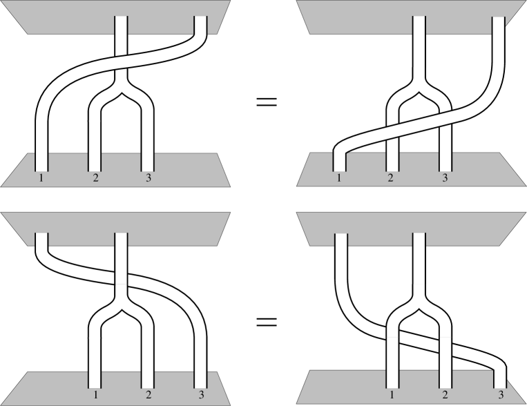
Figure 2.1: Compatibility of fusion and braiding as expressed by the quasitriangularity conditions. It makes no difference whether a third particle braids with two particles separately or with the composite that arises after fusing these two particles. The ribbons represent the trajectories of the particles.

The braid operation is formally implemented by the universal $R$-matrix, which is an element of $D({H})\otimes D({H})$

$$R = \sum_{h,g}\,{\rm P}_{g}\otimes{\rm P}_{h}\,{g}.$$ (2.1.14)

The $R$ matrix acts on a two particle state as a global symmetry transformation on the second particle by the flux of the first particle. The physical braid operator ${\cal R}$ that effectuates a counterclockwise interchange of the two particles is defined as the action of this $R$ matrix followed by a permutation $\sigma$ of the two particles

$${\cal R}_{\alpha\beta}^{AB} := \sigma\circ(\Pi_{\alpha}^{A}\otimes\Pi_{\beta}^{B})(\,R\,),$$ (2.1.15)

To be explicit, on the two particle charge flux eigenstate $|\,^{A}\!h_{i},\,^{\alpha}\!v_{j}\rangle|\,^{B}\!h_{m},\,^{\beta}\!v_{n}\rangle\in V^{A}_{\alpha}\otimes V^{B}_{\beta}$, we have

$${\cal R}\;|\,^{A}\!h_{i},\,^{\alpha}\!v_{j}\rangle|\,^{B}\!h_{m},\,^{\beta}\!v_{n}\rangle = |\,^{A}\!h_{i}\,^{B}\!h_{m}\,^{A}\!h_{i}^{-1},\,\beta(\,^{A}\!\tilde{h}_{i}\,)_{ln}\,^{\beta}\!v_{l}\rangle|\,^{A}\!h_{i},\,^{\alpha}\!v_{j}\rangle,$$ (2.1.16)

where the element ${}^{A}\!\tilde{h}_{i}$ is defined as in (2.1.8). Note that the expression (2.1.16), which summarizes the braid operation on all conceivable two particle states in this theory, contains the braid effects established in section 1.4.2 and 1.4.3, namely flux metamorphosis for two pure magnetic fluxes (1.4.18) and the Aharonov-Bohm effect for a pure magnetic flux with a pure charge (1.4.23).

It is now easily verified that the braid operator defined in (2.1.16) and the comultiplication given by (2.1.12) satisfy the quasitriangularity conditions

$${\cal R}\>\Delta(\,{\rm P}_{h}\,g\,) = \Delta(\,{\rm P}_{h}\,g\,)\>{\cal R}$$ (2.1.17)

$$({\rm id}\otimes\Delta)({\cal R}) = {\cal R}_{2}\;{\cal R}_{1}$$ (2.1.18)

$$(\Delta\otimes{\rm id})({\cal R}) = {\cal R}_{1}\;{\cal R}_{2}.$$ (2.1.19)

Here, the braid operators ${\cal R}_{1}$ and ${\cal R}_{2}$ respectively act as ${\cal R}\otimes{\bf 1}$ and ${\bf 1}\otimes{\cal R}$ on three particle states in the internal Hilbert space $V_{\alpha}^{A}\otimes V_{\beta}^{B}\otimes V_{\gamma}^{C}$. The relation (2.1.17) expresses the fact that the braid operator commutes with the global symmetry transformations $g\in{H}$ and conserves the total magnetic flux of the configuration as measured by ${\rm P}_{h}$. In addition, the quasitriangularity conditions (2.1.18) and (2.1.19), which can be presented graphically as in figure 2.1, imply consistency between braiding and fusing. From the complete set of quasitriangularity conditions, it follows that the braid operator satisfies the Yang-Baxter equation

$${\cal R}_{1}\;{\cal R}_{2}\;{\cal R}_{1} = {\cal R}_{2}\;{\cal R}_{1}\;{\cal R}_{2}.$$ (2.1.20)

Thus the braid operators (2.1.16) define representations of the braid groups discussed in section 1.2. These unitary representations are in general reducible. So the internal Hilbert space describing a multi-particle system in general splits up into a direct sum of irreducible subspaces under the action of the braid group. The braid properties of the system depend on the particular irreducible subspace. If the dimension of the irreducible representation is one, we are dealing with abelian braid statistics or ordinary anyons. If the dimension is larger then one, we are dealing with nonabelian braid statistics, i.e. the nonabelian generalization of anyons. Note that the latter higher dimensional irreducible representations only occur for systems consisting of more than two particles, because the braid group for two particles is abelian.

To conclude, the internal Hilbert space describing a multi-particle system in a discrete $H$ gauge theory carries a representation of the internal symmetry algebra $D({H})$ and a braid group representation. Both representations are in general reducible. The quasitriangularity condition (2.1.17) implies (see for instance [alvarez1, alvarez2]) that the action of the associated braid operators commutes with the action of the elements of $D({H})$. Hence, the multi-dyon internal Hilbert space can in fact be decomposed into a direct sum of irreducible subspaces under the direct product action of $D({H})$ and the braid group. We discuss this in further detail in the next two sections. We first introduce the notion of truncated braid groups.

2.2 Truncated braid groups

We turn to a closer examination of the braid group representations that occur in discrete ${H}$ gauge theories. An important observation in this respect is that the braid operator (2.1.16) is of finite order:

$${\cal R}^{m} = {\bf 1}\otimes{\bf 1},$$ (2.2.1)

with ${\bf 1}$ the identity operator and $m$ some integer depending on the specific particles on which the braid operator acts. In other words, we can assign a finite number $m$ to any two particle internal Hilbert space $V_{\alpha}^{A}\otimes V_{\beta}^{B}$, such that the effect of $m$ braidings is trivial for all states in this internal Hilbert space. This result, which can be traced back directly to the finite order of ${H}$, implies that the multi-particle configurations appearing in a discrete ${H}$ gauge theory actually realize representations of factor groups of the braid groups discussed in section 1.2. Consider, for instance, a system consisting of $n$ indistinguishable particles. Hence, all particles carry the same internal Hilbert space $V^{A}_{\alpha}$ and the $n$ particle internal Hilbert space describing this system is the tensor product space $(V^{A}_{\alpha})^{\otimes n}$. The abstract generator $\tau_{i}$, which establishes a counterclockwise interchange of the two adjacent particles $i$ and $i+1$, acts on this internal Hilbert space by means of the operator

$$\tau_{i} \longmapsto {\cal R}_{i}\,,$$ (2.2.2)

with

$${\cal R}_{i} := {\bf 1}^{\otimes(i-1)}\otimes{\cal R}\otimes{\bf 1}^{\otimes(n-i-1)}.$$ (2.2.3)

That is, the generator $\tau_{i}$ acts as (2.1.16) on the $i^{\rm th}$ and $(i+1)^{\rm th}$ entry in the tensor product space $(V^{A}_{\alpha})^{\otimes n}$. As follows from (2.1.20) and (2.2.1), the homomorphism (2.2.2) furnishes a representation of the braid group

$$\begin{array}[]{rcll}\tau_{i}\tau_{i+1}\tau_{i}&=&\tau_{i+1}\tau_{i}\tau_{i+1}&\qquad i=1,\ldots,n-2\\ \tau_{i}\tau_{j}&=&\tau_{j}\tau_{i}&\qquad|i-j|\geq 2,\end{array}$$ (2.2.6)

with the extra relation

$$\tau_{i}^{m} = e\;\;\;\;\;\;\;\;\;\;i=1,\ldots,n-1,$$ (2.2.7)

where $e$ denotes the unit element or trivial braid. For obvious reasons, we will call the factor groups with defining relations (2.2.6) and the additional relation (2.2.7) truncated braid groups $B(n,m)$. Here $n$ naturally stands for the number of particles and $m$ for the order of the generators $\tau_{i}$.

The observation of the previous paragraph naturally extends to a system containing $n$ distinguishable particles, i.e. the particles carry different internal Hilbert spaces or ‘colors’ now. The group that governs the monodromy properties of such a system is the truncated version $P(n,m)$ of the colored braid group $P_{n}({\bf R}^{2})$ defined in section 1.2. To be specific, the truncated colored braid group $P(n,m)$ is the subgroup of $B(n,m)$ generated by the elements

$$\gamma_{ij} = \tau_{i}\cdots\tau_{j-2}\;\tau_{j-1}^{2}\;\tau_{j-2}^{-1}\cdots\tau_{i}^{-1}\qquad\qquad 1\leq i<j\leq n,$$ (2.2.8)

with the extra relation (2.2.7) incorporated. Thus the generators of the pure braid group satisfy

$$\gamma_{ij}^{m/2} = e,$$ (2.2.9)

from which it is clear that the colored braid group $P(n,m)$ is, in fact, only defined for even $m$. The representation of the colored braid group $P(n,m)$ realized by a system of $n$ different particles in a discrete $H$ gauge theory then becomes

$$\gamma_{ij} \longmapsto {\cal R}_{i}\cdots{\cal R}_{j-1}\;{\cal R}_{j}^{2}\;{\cal R}_{j-1}^{-1}\cdots{\cal R}_{i}^{-1},$$ (2.2.10)

where the operators ${\cal R}_{i}$ defined by expression (2.2.3) now act on the tensor product space $V^{A_{1}}_{\alpha_{1}}\otimes\cdots\otimes V^{A_{n}}_{\alpha_{n}}$ of $n$ different internal Hilbert spaces $V^{A_{l}}_{\alpha_{l}}$ with $l\in 1,2,\ldots,n$.

Finally, a ‘mixture’ of the above systems is of course also possible, that is, a system containing a subsystem consisting of $n_{1}$ particles with ‘color’ $V^{A_{1}}_{\alpha_{1}}$, a subsystem of $n_{2}$ particles carrying the different ‘color’ $V^{A_{2}}_{\alpha_{2}}$ and so on. Such a system realizes a representation of a truncated partially colored braid group (see section 1.2 and the references given there for the definition of ordinary partially colored braid groups). Let $n=n_{1}+n_{2}+\ldots$ again be the total number of particles in the system. The truncated partially colored braid group associated with this system then becomes the subgroup of some truncated braid group $B(n,m)$, generated by the braid operations on particles with the same ‘color’ and the monodromy operations on particles carrying different ‘color’.

The appearance of truncated rather than ordinary braid groups facilitates the decomposition of a given multi-particle internal Hilbert space into irreducible subspaces under the braid/monodromy operations. The point is that the representation theory of ordinary braid groups is rather complicated due to their infinite order. The extra relation (2.2.7) for truncated braid groups $B(n,m)$, however, causes these to become finite for various values of the labels $n$ and $m$, which leads to identifications with well-known groups of finite order [pema]. It is instructive to consider some of these cases explicitly. The truncated braid group $B(2,m)$ for two indistinguishable particles, for instance, has only one generator $\tau$, which satisfies $\tau^{m}=e$. Thus, we obtain the isomorphism

$$B(2,m) \simeq {\bf Z}_{m}.$$ (2.2.11)

For $m=2$, the relations (2.2.6) and (2.2.7) are the defining relations of the permutation group $S_{n}$ on $n$ strands

$$B(n,2) \simeq S_{n}.$$ (2.2.12)

A less trivial example is the nonabelian truncated braid group $B(3,3)$ for 3 indistinguishable particles. By explicit construction from the defining relations (2.2.6) and (2.2.7), we arrive at the identification

$$B(3,3) \simeq \bar{T},$$ (2.2.13)

with $\bar{T}$ the lift of the tetrahedral group into $SU(2)$. The structure of the truncated braid group $B(3,4)$ and its subgroup $P(3,4)$, which for example occur in a $\bar{D}_{2}$ gauge theory (see section 3.3), can be found in appendix LABEL:trubra.

To our knowledge, truncated braid groups have not been studied in the literature so far and a complete classification is not available. An interesting group theoretical question in this context is whether the truncated braid groups are of finite order for all values of the labels $n$ and $m$.

2.3 Fusion, spin, braid statistics and all that $\dots$

Let $(\Pi^{A}_{\alpha},V_{\alpha}^{A})$ and $(\Pi^{B}_{\beta},V_{\beta}^{B})$ be two irreducible representations of the quantum double $D({H})$ as defined in (2.1.7). The tensor product representation $(\Pi^{A}_{\alpha}\otimes\Pi^{B}_{\beta},V_{\alpha}^{A}\otimes V_{\beta}^{B})$, constructed by means of the comultiplication (2.1.12), need not be irreducible. In general, it gives rise to a decomposition

$$\Pi^{A}_{\alpha}\otimes\Pi^{B}_{\beta} = \bigoplus_{C,\gamma}N^{AB\gamma}_{\alpha\beta C}\;\Pi^{C}_{\gamma},$$ (2.3.1)

where $N^{AB\gamma}_{\alpha\beta C}$ stands for the multiplicity of the irreducible representation $(\Pi^{C}_{\gamma},V^{C}_{\gamma})$. From the orthogonality relation for the characters of the irreducible representations of $D({H})$, we infer [dpr]

$$N^{AB\gamma}_{\alpha\beta C} = \frac{1}{|{H}|}\sum_{h,g}\;\mbox{tr}\left(\Pi^{A}_{\alpha}\otimes\Pi^{B}_{\beta}(\Delta(\,{\rm P}_{h}\,g\,))\right)\;\mbox{tr}\left(\Pi^{C}_{\gamma}(\,{\rm P}_{h}\,g\,)\right)^{*},$$ (2.3.2)

where $|{H}|$ denotes the order of the group ${H}$ and $*$ indicates complex conjugation. The fusion rule (2.3.1) now determines which particles $(\,^{C}C,\gamma)$ can be formed in the composition of two given particles $(\,^{A}C,\alpha\,)$ and $(\,^{B}C,\beta\,)$, or if read backwards, gives the decay channels of the particle $(\,^{C}C,\gamma\,)$.

The fusion algebra, spanned by the elements $\Pi^{A}_{\alpha}$ with multiplication rule (2.3.1), is commutative and associative and can therefore be diagonalized. The matrix implementing this diagonalization is the so-called modular $S$ matrix [ver0]

$$S^{AB}_{\alpha\beta} := \frac{1}{|{H}|}\,\mbox{tr}\;{\cal R}^{-2\;AB}_{\;\;\;\;\;\alpha\beta}$$

$$= \frac{1}{|{H}|}\,\sum_{\stackrel{{\,{}^{A}\!h_{i}\in\,^{A}\!C\,,^{B}\!h_{j}\in\,^{B}\!C}}{{[\,^{A}\!h_{i},\,^{B}\!h_{j}]=e}}}\mbox{tr}\left(\alpha(\,^{A}\!x_{i}^{-1}\,{}^{B}\!h_{j}\,^{A}\!x_{i})\right)^{*}\;\mbox{tr}\left(\beta(\,^{B}\!x_{j}^{-1}\,{}^{A}\!h_{i}\,^{B}\!x_{j})\right)^{*},$$

The modular $S$ matrix (2.3) contains all information concerning the fusion algebra defined in (2.3.1). In particular, the multiplicities (2.3.2) can be expressed in terms of the modular $S$ matrix by means of Verlinde’s formula [ver0]

$$N^{AB\gamma}_{\alpha\beta C} = \sum_{D,\delta}\frac{S^{AD}_{\alpha\delta}S^{BD}_{\beta\delta}(S^{*})^{CD}_{\gamma\delta}}{S^{eD}_{0\delta}}.$$ (2.3.4)

Whereas the modular $S$ matrix is determined through the monodromy operator following from (2.1.16), the modular matrix $T$ contains the spin factors (2.1.11) assigned to the particles in the spectrum of a discrete $H$ gauge theory

$$T^{AB}_{\alpha\beta} := \delta_{\alpha,\beta}\,\delta^{A,B}\;\exp(2\pi\imath s_{(A,\alpha)})\;=\;\delta_{\alpha,\beta}\,\delta^{A,B}\frac{1}{d_{\alpha}}\,\mbox{tr}\left(\alpha(^{A}\!h_{1})\right),$$ (2.3.5)

where $d_{\alpha}$ stands for the dimension of the centralizer charge representation $\alpha$ of the particle $(\,^{A}C,\alpha\,)$. The matrices (2.3) and (2.3.5) now realize an unitary representation of the modular group $SL(2,{\bf Z})$ with the following relations [dvvv]

$$\halign to=0.0pt{\hskip\@centering$\displaystyle{#}$\@eqnsel&\global\@eqcnt\@ne\hskip\tw@\arraycolsep\hfil${#}$\hfil&\global\@eqcnt\tw@\hskip\tw@\arraycolsep$\displaystyle{#}$\hfil&\global\@eqcnt\thr@@\hskip\tw@\arraycolsep\hfil\hbox{#}&\global\@eqcnt 4 \hbox\bgroup\hss#\egroup\cr 0.0pt plus 1000.0pt$\displaystyle{{\cal C} &10.0pt\hfil${=&10.0pt$\displaystyle{(ST)^{3} \; = \; S^{2}, &10.0pt\hfil\hbox{ \\ S^* &{\hss=}&{\cal C}S\;=\;S^{-1},&$\qquad S^t \;=\; S, $\\T^{*}&=&T^{-1},&$\qquad T^t \;=\; T.$(2.3.6)\cr}}}}}$$

The relations (2.3) and (2.3) express the fact that the matrices (2.3) and (2.3.5) are symmetric and unitary. To proceed, the matrix ${\cal C}$ defined in (2.3) represents the charge conjugation operator, which assigns an unique anti-partner ${\cal C}\,(\,^{A}C,\alpha\,)=(\,^{\bar{A}}C,\bar{\alpha}\,)$ to each particle $(\,^{A}C,\alpha\,)$ in the spectrum, such that the vacuum channel occurs in the fusion rule (2.3.1) for the particle/anti-particle pairs. Also, note that the complete set of relations imply that the charge conjugation matrix ${\cal C}$ commutes with the modular matrix $T$, which implies that a given particle carries the same spin as its anti-partner.

Having determined the fusion rules and the associated modular algebra, we turn to the issue of braid statistics and the fate of the spin statistics connection in nonabelian discrete $H$ gauge theories. Let us emphasize from the outset that much of what follows has been established elsewhere in a more general setting. See [alvarez1, alvarez2, moseco] and the references therein for the conformal field theory point of view and [frohma, frogama, witten] for the related 2+1 dimensional space time perspective.

We first discuss a system consisting of two distinguishable particles $(\,^{A}C,\alpha\,)$ and $(\,^{B}C,\beta\,)$. The associated two particle internal Hilbert space $V_{\alpha}^{A}\otimes V_{\beta}^{B}$ carries a representation of the abelian truncated colored braid group $P(2,m)$ with $m/2\in{\bf Z}$ the order of the monodromy matrix ${\cal R}^{2}$ for this particular two-particle system. This representation decomposes into a direct sum of one dimensional irreducible subspaces, each being labeled by the associated eigenvalue of the monodromy matrix ${\cal R}^{2}$. Recall from section 2.1, that the monodromy operation commutes with the action of the quantum double. This implies that the decomposition (2.3.1) simultaneously diagonalizes the monodromy matrix. To be specific, the two particle total flux/charge eigenstates spanning a given fusion channel $V_{\gamma}^{C}$ all carry the same monodromy eigenvalue, which in addition can be shown to satisfy the generalized spin-statistics connection [dpr]

$$K^{ABC}_{\alpha\beta\gamma}\;{\cal R}^{2} = e^{2\pi\imath(s_{(C,\gamma)}-s_{(A,\alpha)}-s_{(B,\beta)})}\;\;K^{ABC}_{\alpha\beta\gamma}.$$ (2.3.7)

Here, $K^{ABC}_{\alpha\beta\gamma}$ stands for the projection on the irreducible component $V_{\gamma}^{C}$ of $V_{\alpha}^{A}\otimes V_{\beta}^{B}$. In other words, the monodromy operation on a two particle state in a given fusion channel is the same as a clockwise rotation over an angle of $2\pi$ of the two particles separately accompanied by a counterclockwise rotation over an angle of $2\pi$ of the single particle state emerging after fusion. This is consistent with the observation that these two processes can be continuously deformed into each other, see the associated ribbon diagrams depicted in figure 2.2. The discussion can now be summarized by the statement that the total internal Hilbert space $V_{\alpha}^{A}\otimes V_{\beta}^{B}$ decomposes into the following direct sum of irreducible representations of the direct product $D({H})\times P(2,m)$

$$\bigoplus_{C,\gamma}N^{AB\gamma}_{\alpha\beta C}\;(\Pi^{C}_{\gamma},\Lambda_{C-A-B}),$$ (2.3.8)

where $\Lambda_{C-A-B}$ denotes the one dimensional irreducible representation of $P(2,m)$ in which the monodromy generator $\gamma_{12}$ acts as (2.3.7).

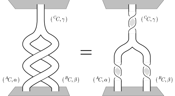
Figure 2.2: Generalized spin-statistics connection. The displayed ribbon diagrams are homotopic as can be checked with the pair of pants you are presently wearing. This means that a monodromy of two particles in a given fusion channel followed by fusion of the pair can be continuously deformed into the process describing a rotation over an angle of $-2\pi$ of the two particles seperately followed by fusion of the pair and a final rotation over an angle of $2\pi$ of the composite.

The analysis for a configuration of two indistinguishable particles $(\,^{A}C,\alpha\,)$ is analogous. The total internal Hilbert space $V_{\alpha}^{A}\otimes V_{\alpha}^{A}$ decomposes into one dimensional irreducible subspaces under the action of the truncated braid group $B(2,m)$ with $m$ the order of the braid operator ${\cal R}$, which depends on the system under consideration. By the same argument as before, the two particle total flux/charge eigenstates spanning a given fusion channel $V_{\gamma}^{C}$ all carry the same one dimensional representation of $B(2,m)$. The quantum statistical parameter assigned to this channel now satisfies the square root version of the generalized spin-statistics connection (2.3.7)

$$K^{AAC}_{\alpha\alpha\gamma}\;{\cal R} = \epsilon\;e^{\pi\imath(s_{(C,\gamma)}-2s_{(A,\alpha)})}\;\;K^{AAC}_{\alpha\alpha\gamma},$$ (2.3.9)

with $\epsilon$ a sign depending on whether the fusion channel $V_{\gamma}^{C}$ appears in a symmetric or an anti-symmetric fashion [alvarez1, alvarez2]. In other words, the internal space Hilbert space for a system of two indistinguishable particles $(\,^{A}C,\alpha\,)$ breaks up into the following irreducible representations of the direct product $D(H)\times B(2,m)$

$$\bigoplus_{C,\gamma}N^{AA\gamma}_{\alpha\alpha C}\;(\Pi^{C}_{\gamma},\Lambda_{C-2A}),$$ (2.3.10)

with $\Lambda_{C-2A}$ the one dimensional representation of the truncated braid group $B(2,m)$ defined in (2.3.9).

The result (2.3.9) is actually rather surprising. It states that indistinguishable particle systems in a nonabelian discrete $H$ gauge theory quite generally violate the canonical spin-statistics connection (1.3.40). More accurately, in a nonabelian discrete gauge theory we are dealing with the generalized connection (2.3.9), which incorporates the canonical one. In fact, the canonical spin-statistics connection is retrieved in some particular channels occurring in (2.3.10), as we will argue now. Let us first emphasize that the basic assertions for the ribbon proof depicted in figure 1.7 are naturally satisfied in the nonabelian setting as well. For every particle $(\,^{A}C,\alpha\,)$ in the spectrum there exists an anti-particle $(\,^{\bar{A}}C,\bar{\alpha}\,)$ such that under the proper composition the pair acquires the quantum numbers of the vacuum and may decay. Moreover, every particle carries the same spin as its anti-partner, as indicated by the fact that the charge conjugation operator ${\cal C}$ commutes with the modular matrix $T$. It should be noted now that the ribbon proof in figure 1.7 actually only applies to states in which the particles that propagate along the exchanged ribbons are in strictly identical internal states. Otherwise the ribbons can not be closed. Indeed, we find that the action (2.1.16) of the braid operator on two particles in identical internal flux/charge eigenstates

$${\cal R}\;|\,^{A}\!h_{i},\,^{\alpha}\!v_{j}\rangle|\,^{A}\!h_{i},\,^{\alpha}\!v_{j}\rangle = |\,^{A}\!h_{i},\,\alpha\,(\,^{A}\!h_{1}\,)_{mj}\,^{\alpha}\!v_{j}\rangle|\,^{A}\!h_{i},\,^{\alpha}\!v_{j}\rangle,$$ (2.3.11)

boils down to the diagonal matrix (2.1.11) and therefore to the same spin factor (2.3.12) for all $i,j$

$$\exp(\imath\Theta_{(A,\alpha)}) = \exp(2\pi\imath s_{(A,\alpha)}).$$ (2.3.12)

The conclusion is that the canonical spin-statistics connection is restored in the fusion channels spanned by linear combinations of the states (2.3.11) in which the particles are in strictly identical internal flux/charge eigenstates. The quantum statistical parameter (2.3.9) assigned to these channels reduces to the spin factor (2.3.12). Thus the effect of a counterclockwise interchange of the two particles in the states in these channels is the same as the effect of rotating one of the particles over an angle of $2\pi$. To conclude, the closed ribbon proof does not apply to the other channels and we are left with the more involved connection (2.3.9) following from the open ribbon argument displayed in figure 2.2.

Finally, higher dimensional irreducible braid group representations are conceivable for a system which consists of more than two particles. The occurrence of such representations simply means that the generators of the braid group can not be diagonalized simultaneously. What happens in this situation is that under the full set of braid operations, the system jumps between isotypical fusion channels, i.e. fusion channels of the same type or ‘color’. Let us make this statement more precise. To keep the discussion general, we do not specify the nature of the particles in the system. Depending on whether the system consists of distinguishable particles, indistinguishable particles or some ‘mixture’, we are dealing with a truncated braid group, a colored braid group or a partially colored braid group respectively. The internal Hilbert for such a system again decomposes into a direct sum of irreducible subspaces (or fusion channels) under the action of the quantum double $D(H)$. Given the fact that the action of the associated braid group commutes with that of the quantum double, we are left with two possibilities. First of all, there will in general be some fusion channels separately being invariant under the action of the full braid group. As in the two particle systems discussed before, the total flux/charge eigenstates spanning such a fusion channel, say $V_{\gamma}^{C}$, carry the same one dimensional irreducible representation $\Lambda_{ab}$ of the braid group. That is, these states realize abelian braid statistics with the same quantum statistical parameter. The fusion channel $V_{\gamma}^{C}$ then carries the irreducible representation $(\Pi_{\gamma}^{C},\Lambda_{ab})$ of the direct product of the quantum double and the braid group. In addition, it is also feasible that states carrying the same total flux and charge in different (isotypical) fusion channels are mixed under the action of the full braid group. In that case, we are dealing with a higher dimensional irreducible representation of the truncated braid group or nonabelian braid statistics. Note that nonabelian braid statistics is conceivable, if and only if some fusion channel, say $V_{\delta}^{D}$, occurs more then once in the decomposition of the Hilbert space under the action of the quantum double. Only then there are some orthogonal states with the same total flux and charge available to span an higher dimensional irreducible representation of the braid group. The number $n$ of fusion channels $V_{\delta}^{D}$ related by the action of the braid operators now constitutes the dimension of the irreducible representation $\Lambda_{nonab}$ of the braid group and the multiplicity of this representation is the dimension $d$ of the fusion channel $V_{\delta}^{D}$. To conclude, the direct sum of these $n$ fusion channels $V_{\delta}^{D}$ carries an $n\cdot d$ dimensional irredicible representation $(\Pi_{\delta}^{D},\Lambda_{nonab})$ of the direct product of the quantum double and the braid group.

Chapter 3 $\bar{D}_{2}$ gauge theory

In this last chapter, we will illustrate the foregoing general considerations with one of the simplest nonabelian discrete ${H}$ gauge theories, namely that with finite gauge group the double dihedral group ${H}\simeq\bar{D}_{2}$. See also the references [spm, spm1, sm] in this connection. The plan is as follows. In section 3.1, we establish the spectrum of a $\bar{D}_{2}$ gauge theory, the spin factors assigned to the particles and the fusion rules. Here, we also elaborate on a feature special for nonabelian discrete ${H}$ gauge theories: a pair of nonabelian magnetic fluxes can carry charges that are not localized on any of the two fluxes nor anywhere else. Among other things, we will show that these so-called Cheshire charges a nonabelian flux pair may carry, can be excited by monodromy processes with other particles in the spectrum. In section 3.2, we treat the (nonabelian) cross sections measured in Aharonov-Bohm scattering experiments involving the particles in a $\bar{D}_{2}$ gauge theory. Further, the issue of (nonabelian) braid statistics realized by the multi-particle configurations in this theory will be dealt with in section 3.3. We have also included two appendices. Appendix LABEL:ahboverl contains a concise review of the Aharonov-Bohm scattering experiment focussing on the cross sections appearing in (non)abelian discrete $H$ gauge theories. Finally, in appendix LABEL:trubra, we give the group structure of two particular truncated braid groups which enter the analysis in section 3.3.

3.1 Alice in physics

A $\bar{D}_{2}$ gauge theory may, for instance, arise as ‘the long distance remnant’ of a Higgs model of the form (1.4.22) in which the gauge group $G\simeq SU(2)$ is spontaneously broken down to the double dihedral group $H\simeq\bar{D}_{2}\subset SU(2)$. Since $SU(2)$ is simply connected, the fundamental group $\pi_{1}(SU(2)/\bar{D}_{2})$ coincides with the residual symmetry group $\bar{D}_{2}$. Hence, the stable magnetic fluxes in this broken theory are indeed labeled by the group elements of $\bar{D}_{2}$. See the discussion concerning the isomorphism (1.4.3) in section 1.4.1. In the following, we will not dwell any further on the explicit details of this or other possible embeddings in broken gauge theories and simply focus on the features of the $\bar{D}_{2}$ gauge theory itself. We start with a discussion of the spectrum.

Conjugacy class		Centralizer
$e=\{e\}$		$\qquad\bar{D}_{2}$
$\bar{e}=\{\bar{e}\}$		$\qquad\bar{D}_{2}$
$X_{1}=\{X_{1},\bar{X}_{1}\}\$		$\qquad{\bf Z}_{4}\simeq\{e,X_{1},\bar{e},\bar{X}_{1}\}$
$X_{2}=\{X_{2},\bar{X}_{2}\}$		$\qquad{\bf Z}_{4}\simeq\{e,X_{2},\bar{e},\bar{X}_{2}\}$
$X_{3}=\{X_{3},\bar{X}_{3}\}$		$\qquad{\bf Z}_{4}\simeq\{e,X_{3},\bar{e},\bar{X}_{3}\}$

Table 3.1: Conjugacy classes of the double dihedral group $\bar{D}_{2}$ together with their centralizers.

$\rule{0.0pt}{9.95845pt}\bar{D}_{2}\qquad$	$e$	$\bar{e}$	$X_{1}$	$X_{2}$	$X_{3}$
$1\rule{0.0pt}{9.95845pt}$	$1$	$1$	$1$	$1$	$1$
$J_{1}\rule{0.0pt}{9.95845pt}$	$1$	$1$	$1$	$-1$	$-1$
$J_{2}\rule{0.0pt}{9.95845pt}$	$1$	$1$	$-1$	$1$	$-1$
$J_{3}\rule{0.0pt}{9.95845pt}$	$1$	$1$	$-1$	$-1$	$1$
$\chi\rule{0.0pt}{9.95845pt}$	$2$	$-2$	$0$	$0$	$0$

$\rule{0.0pt}{9.95845pt}{\bf Z}_{4}\qquad$	$e$	$X_{a}$	$\bar{e}$	$\bar{X}_{a}$
${\Gamma^{0}}\rule{0.0pt}{9.95845pt}$	$1$	$1$	$1$	$1$
${\Gamma^{1}}\rule{0.0pt}{9.95845pt}$	$1$	$\imath$	$-1$	$-\imath$
${\Gamma^{2}}\rule{0.0pt}{9.95845pt}$	$1$	$-1$	$1$	$-1$
${\Gamma^{3}}\rule{0.0pt}{9.95845pt}$	$1$	$-\imath$	$-1$	$\imath$

Table 3.2: Character tables of $\bar{D}_{2}$ and ${\bf Z}_{4}$.

The double dihedral group $\bar{D}_{2}$ is a group of order $8$ with a nontrivial centre of order $2$. The magnetic fluxes associated with its group elements are organized in the conjugacy classes exhibited in table 3.1. There are five conjugacy classes which we will denote as $e,\bar{e},X_{1},X_{2}$ and $X_{3}$. The conjugacy class $e$ naturally corresponds to the trivial magnetic flux sector, while the conjugacy class $\bar{e}$ consists of the nontrivial centre element. The conjugacy classes $X_{1},X_{2}$ and $X_{3}$ all contain two commuting elements of order $4$. In other words, a $\bar{D}_{2}$ gauge theory features four nontrivial purely magnetic flux sectors: one singlet flux $\bar{e}$ and three different doublet fluxes $X_{1},X_{2}$ and $X_{3}$. The purely electric charge sectors, on the other hand, correspond to the UIR’s of $\bar{D}_{2}$. From the character table displayed in table 3.2, we infer that there are four nontrivial pure charges in the spectrum: three singlet charges $J_{1},J_{2},J_{3}$ and one doublet charge $\chi$. The magnetic fluxes $X_{a}$ and $\bar{X}_{a}$ (with $a\in 1,2,3$) act on the doublet charge $\chi$ as $\imath\sigma_{a}$ and $-\imath\sigma_{a}$, respectively, where the symbol $\sigma_{a}$ denotes the Pauli matrices. Let us now turn to the dyonic sectors. These are constructed by assigning a nontrivial centralizer representation to the nontrivial fluxes. The centralizers associated with the different flux sectors can be found in table 3.1. The flux $\bar{e}$ obviously commutes with the full group $\bar{D}_{2}$, while the centralizer of the other flux sectors is the cyclic group ${\bf Z}_{4}$. Hence, we arrive at thirteen different dyons: three singlet dyons and one doublet dyon associated with the flux $\bar{e}$ and nine doublets dyons associated with the fluxes $X_{1},X_{2}$ and $X_{3}$ paired with nontrivial ${\bf Z}_{4}$ representations. All in all, the spectrum of this theory features 22 particles, which will be labeled as

$$\begin{array}[]{rclrcl}1&:=&(e,\,1)&\qquad\qquad\bar{1}&:=&(\bar{e},\,1)\\ J_{a}&:=&(e,\,J_{a})&\qquad\qquad\bar{J}_{a}&:=&(\bar{e},\,J_{a})\\ \chi&:=&(e,\,\chi)&\qquad\qquad\bar{\chi}&:=&(\bar{e},\,\chi)\\ \sigma_{a}^{+}&:=&(X_{a},\,{\Gamma^{0}})&\qquad\qquad\sigma_{a}^{-}&:=&(X_{a},\,{\Gamma^{2}})\\ \tau_{a}^{+}&:=&(X_{a},\,{\Gamma^{1}})&\qquad\qquad\tau_{a}^{-}&:=&(X_{a},\,{\Gamma^{3}}),\end{array}$$ (3.1.6)

for convenience. Note that the square of the dimensions of the internal Hilbert spaces carried by these particles indeed add up to the order of the quantum double $D(\bar{D}_{2})$: $8\cdot 1^{2}+14\cdot 2^{2}=8^{2}$.

As has been argued in section 2.3, the topological interactions described by a discrete ${H}$ gauge theory are encoded in the associated modular matrices $S$ and $T$. The modular $T$ matrix (2.3.5) contains the spin factors assigned to the different particles. With relation (2.1.11) and table 3.2, we easily infer the following spin factors for the particles in the spectrum (3.1.6) of a $\bar{D}_{2}$ gauge theory

$$\begin{array}[]{cc}\mbox{particle}&\qquad\exp(2\pi\imath s)\\ 1,J_{a}&\qquad 1\\ \bar{1},\bar{J}_{a}&\qquad 1\\ \chi,\bar{\chi}&\qquad 1,-1\\ \sigma_{a}^{\pm}&\qquad\pm 1\\ \tau_{a}^{\pm}&\qquad\pm\imath.\end{array}$$ (3.1.13)

The modular $S$ matrix (2.3), on the other hand, is determined by the monodromy matrix following from (2.1.16). A lengthy but straightforward calculation shows that the modular $S$ matrix for a $\bar{D}_{2}$ gauge theory takes the form displayed in table 3.3. We proceed by enumerating the fusion rules following from plugging this modular $S$ matrix in Verlinde’s formula (2.3.4).

$S$		$1$	$\bar{1}$	$J_{a}$	$\bar{J}_{a}$	$\chi$	$\bar{\chi}$	$\sigma^{+}_{a}$	$\sigma^{-}_{a}$	$\tau^{+}_{a}$	$\tau^{-}_{a}$
$1$		$1$	$1$	$1$	$1$	$2$	$2$	$2$	$2$	$2$	$2$
$\bar{1}$		$1$	$1$	$1$	$1$	$-2$	$-2$	$2$	$2$	$-2$	$-2$
$J_{b}$		$1$	$1$	$1$	$1$	$2$	$2$	$2\epsilon_{ab}$	$2\epsilon_{ab}$	$2\epsilon_{ab}$	$2\epsilon_{ab}$
$\bar{J}_{b}$		$1$	$1$	$1$	$1$	$-2$	$-2$	$2\epsilon_{ab}$	$2\epsilon_{ab}$	$-2\epsilon_{ab}$	$-2\epsilon_{ab}$
$\chi$		$2$	$-2$	$2$	$-2$	$4$	$-4$	$0$	$0$	$0$	$0$
$\bar{\chi}$		$2$	$-2$	$2$	$-2$	$-4$	$4$	$0$	$0$	$0$	$0$
$\sigma^{+}_{b}$		$2$	$2$	$2\epsilon_{ab}$	$2\epsilon_{ab}$	$0$	$0$	$4\delta_{ab}$	$-4\delta_{ab}$	$0$	$0$
$\sigma^{-}_{b}$		$2$	$2$	$2\epsilon_{ab}$	$2\epsilon_{ab}$	$0$	$0$	$-4\delta_{ab}$	$4\delta_{ab}$	$0$	$0$
$\tau^{+}_{b}$		$2$	$-2$	$2\epsilon_{ab}$	$-2\epsilon_{ab}$	$0$	$0$	$0$	$0$	$-4\delta_{ab}$	$4\delta_{ab}$
$\tau^{-}_{b}$		$2$	$-2$	$2\epsilon_{ab}$	$-2\epsilon_{ab}$	$0$	$0$	$0$	$0$	$4\delta_{ab}$	$-4\delta_{ab}$

Table 3.3: Modular S-matrix of the quantum double $D(\bar{D}_{2})$ up to an overall factor $\frac{1}{8}$. We defined $\epsilon_{ab}:=1$ iff $a=b$ and $\epsilon_{ab}:=-1$ iff $a\neq b$.

The fusion rules for the purely electric charges are, of course, dictated by the representation ring of $\bar{D}_{2}$

$$J_{a}\times J_{a}=1,\qquad J_{a}\times J_{b}=J_{c},\qquad J_{a}\times\chi=\chi,\qquad\chi\times\chi=1+\sum_{a}J_{a}.$$ (3.1.14)

Here, the subscripts $a,b$ and $c$ take the values $1,2$ or $3$ and where by convention $a\neq b$, $a\neq c$ and $b\neq c$. The latter convention will be used throughout the following. To continue, the dyons associated with the flux $\bar{1}$ are obtained by simply composing this flux with the purely electric charges

$$J_{a}\times\bar{1}=\bar{J}_{a},\qquad\chi\times\bar{1}=\bar{\chi}.$$ (3.1.15)

In a similar fashion, we construct the other dyons

$$J_{a}\times\sigma^{+}_{a}=\sigma^{+}_{a},\qquad J_{b}\times\sigma^{+}_{a}=\sigma^{-}_{a},\qquad\chi\times\sigma^{+}_{a}=\tau^{+}_{a}+\tau^{-}_{a}.$$ (3.1.16)

We now have produced all the constituents of the spectrum as given in (3.1.6). Recall from section 2.3 that the fusion algebra is commutative and associative. This implies that the full set of fusion rules is, in fact, completely determined by a minimal subset. Bearing this in mind, amalgamation involving the flux $\bar{1}$ is unambiguously prescribed by (3.1.15) and

$$\bar{1}\times\bar{1}=1,\qquad\bar{1}\times\sigma^{\pm}_{a}=\sigma^{\pm}_{a},\qquad\bar{1}\times\tau^{\pm}_{a}=\tau^{\mp}_{a}.$$ (3.1.17)

The complete set of fusion rules is then fixed by the previous ones together with

$$J_{a}\times\tau^{\pm}_{a}=\tau^{\pm}_{a},\qquad J_{b}\times\tau^{\pm}_{a}=\tau^{\mp}_{a},\qquad\chi\times\tau^{\pm}_{a}=\sigma^{+}_{a}+\sigma^{-}_{a},$$ (3.1.18)

and

$$\sigma^{s}_{a}\times\sigma^{s}_{a} = 1+J_{a}+\bar{1}+\bar{J}_{a}$$ (3.1.19)

$$\sigma^{s}_{a}\times\sigma^{s}_{b} = \sigma^{+}_{c}+\sigma^{-}_{c}$$ (3.1.20)

$$\sigma^{s}_{a}\times\tau^{s}_{a} = \chi+\bar{\chi}$$ (3.1.21)

$$\sigma^{s}_{a}\times\tau^{s}_{b} = \tau^{+}_{c}+\tau^{-}_{c}$$ (3.1.22)

$$\tau^{s}_{a}\times\tau^{s}_{a} = 1+J_{a}+\bar{J}_{b}+\bar{J}_{c}$$ (3.1.23)

$$\tau^{s}_{a}\times\tau^{s}_{b} = \sigma^{+}_{c}+\sigma^{-}_{c}\,,$$ (3.1.24)

with $s\in+,-$.

A few remarks concerning this fusion algebra are pertinent. First of all, it is easily verified that the class algebra of $\bar{D}_{2}$ is respected as an overall selection rule. The class multiplication in the fusion rule (3.1.19), for instance, reads $X_{a}*X_{a}=2e+2\bar{e}$. The appearance of the class algebra naturally expresses magnetic flux conservation: in establishing the fusion rule, all fluxes in the consecutive conjugacy classes are multiplied out. Further, the modular $S$ matrix as given in table 3.3 is real and therefore equal to its inverse as follows directly from relation (2.3). Consequently, the charge conjugation operator ${\cal C}$ is trivial, i.e. it acts on the spectrum (3.1.6) as the unit matrix ${\cal C}=S^{2}={\bf 1}$. Hence, all particles in this $\bar{D}_{2}$ gauge theory feature as their own anti-particle. Only two similar particles are able to annihilate, as witnessed by the occurrence of the vacuum channel $1$ in the fusion rule for two similar particles.

At first sight, the message of the fusion rule (3.1.19) is actually rather remarkable. It seems that the fusion of two pure fluxes $\sigma_{a}^{+}$ may give rise to electric charge creation. One could start wondering about electric charge conservation at this point. Electric charge is conserved though. Before fusion this charge was present in the form of so-called nonlocalizable Cheshire charge [alice, spm, sm, preskra], i.e. the nontrivial representation of the global symmetry group $\bar{D}_{2}$ carried by the flux pair. This becomes clear upon writing the fusion rule (3.1.19) in terms of the two particle flux states corresponding to the different channels:

$$\frac{1}{\sqrt{2}}\{|\bar{X}_{a}\rangle|X_{a}\rangle\;+\;|X_{a}\rangle|\bar{X}_{a}\rangle\} \longmapsto 1$$ (3.1.25)

$$\frac{1}{\sqrt{2}}\{|\bar{X}_{a}\rangle|X_{a}\rangle\;-\;|X_{a}\rangle|\bar{X}_{a}\rangle\} \longmapsto J_{a}$$ (3.1.26)

$$\frac{1}{\sqrt{2}}\{|X_{a}\rangle|X_{a}\rangle\;+\;|\bar{X}_{a}\rangle|\bar{X}_{a}\rangle\} \longmapsto \bar{1}$$ (3.1.27)

$$\frac{1}{\sqrt{2}}\{|X_{a}\rangle|X_{a}\rangle\;-\;|\bar{X}_{a}\rangle|\bar{X}_{a}\rangle\} \longmapsto \bar{J}_{a}.$$ (3.1.28)

The identification of the two particle flux states at the l.h.s. with the single particle states at the r.h.s. is established by the action (2.1.12) of the quantum double $D(\bar{D}_{2})$ on the two particle states. On the one hand, we can perform global $\bar{D}_{2}$ symmetry transformations from which we learn the total charge carried by the flux pair. As indicated by the comultiplication (2.1.12), the global $\bar{D}_{2}$ transformations act through overall conjugation. The total flux of the pair, on the other hand, is formally obtained by applying the flux projection operators (2.1.1) and is nothing but the product of the two fluxes of the pair. Since $X_{a}\cdot\bar{X}_{a}=e$, the total flux of the two particle state in (3.1.25), for instance, vanishes. Moreover, it is easily verified that this state is invariant under global under global $\bar{D}_{2}$ transformations. Thus it corresponds to the vacuum channel $1$. In a similar fashion, we obtain the identification of the other two particle states with the single particle states. Note that these two particle quantum states describing the flux pairs are nonseparable. The two fluxes are correlated: by measuring the flux of one particle of the pair, we instantaneously fix the flux of the other. This is the famous Einstein-Podolsky-Rosen (EPR) paradox [epr]. Just as in the notorious experiment with two spin $1/2$ particles in the singlet state, it is no longer possible to make a flux measurement on one particle without affecting the other instantaneously. The Cheshire charge carried by the flux pair depends on the symmetry properties of these nonseparable quantum states. The symmetric quantum states correspond to the trivial charge $1$, whereas the anti-symmetric quantum states carry the nontrivial charge $J_{a}$. It is clear that the charge $J_{a}$ can not be localized on any of the fluxes nor anywhere else. It is a property of the pair and only becomes localized when the fluxes are brought together in a fusion process. It is this elusive nature, reminiscent of the smile of the Cheshire cat in Alice’s adventures in wonderland [carroll], that formed the motivation to call such a charge Cheshire charge [colem, preskra].

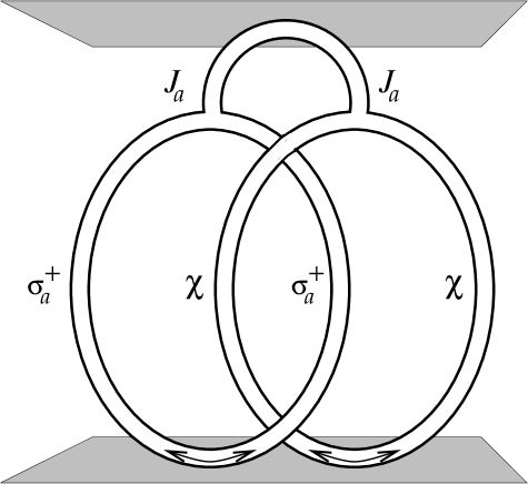
Figure 3.1: A charge/anti-charge pair $\chi$ and a flux/anti-flux pair $\sigma_{a}^{+}$ are created from the vacuum at a certain time slice. The ribbons represent the worldlines of the particles. After the charge $\chi$ has encircled the flux $\sigma_{a}^{+}$, both particle/anti-particle pairs carry the nonlocalizable Cheshire charge $J_{a}$. These Cheshire charges become localized upon rejoining the members of the pairs. Subsequently, the two charges $J_{a}$ annihilate each other.

The Cheshire charge $J_{a}$ of the flux pair can be excited by encircling one flux in the pair by the doublet charge $\chi$ [colem, sm, preskra]. Here, we draw on a further analogy with Alice’s adventures. The magnetic fluxes $X_{a}$ and $\bar{X}_{a}$ act by means of $\imath\sigma_{a}$ and $-\imath\sigma_{a}$ respectively on the doublet charge $\chi$, where the symbol $\sigma_{a}$ denotes the Pauli matrices. This means that when a charge $\chi$ with its orientation down is adiabatically transported around, for example, the flux $X_{2}$, it returns with its orientation up:

$${\cal R}^{2}\;|X_{2}\rangle|\left(\begin{array}[]{c}0\\ 1\end{array}\right)\rangle = |X_{2}\rangle|\left(\begin{array}[]{c}1\\ 0\end{array}\right)\rangle,$$ (3.1.33)

as follows from (2.1.16). In terms of Alice’s adventures: the charge has gone through the looking-glass. For this reason the flux $X_{2}$ has been called an Alice flux [alice, preskra, schwarz]. The other fluxes $X_{a},\bar{X}_{a}$ affect the doublet charge $\chi$ in a similar way. Let us now consider the process depicted in figure 3.1. We start with the creation of a charge/anti-charge pair $\chi$ and a flux/anti-flux pair $\sigma_{a}^{+}$ from the vacuum. Thus both pairs do not carry Cheshire charge at this stage. They are in the vacuum channel of the corresponding fusion rules (3.1.14) and (3.1.19). Next, one member of the charge pair encircles a flux in the flux pair. The flip of the charge orientation (3.1.33) leads to an exchange of the internal quantum numbers of the pairs: both pairs carry Cheshire charge $J_{a}$ after this process, i.e. both pairs are in the $J_{a}$ channel of the associated fusion rules. The global charge of the configuration is conserved. Both charges $J_{a}$ can be annihilated by bringing them together as follows from the fusion rule $J_{a}\times J_{a}=1$ given in (3.1.14). These phenomena can be made explicit by writing this process in terms of the corresponding correlated internal quantum states:

$$1 \longmapsto \frac{1}{2}\{|\bar{X}_{2}\rangle|X_{2}\rangle\;+\;|X_{2}\rangle|\bar{X}_{2}\rangle\}\{|\left(\begin{array}[]{c}1\\ 0\end{array}\right)\rangle|\left(\begin{array}[]{c}0\\ 1\end{array}\right)\rangle\;-\;|\left(\begin{array}[]{c}0\\ 1\end{array}\right)\rangle|\left(\begin{array}[]{c}1\\ 0\end{array}\right)\rangle\}$$ (3.1.42)

$$\stackrel{{\scriptstyle{\bf 1}\otimes{\cal R}^{2}\otimes{\bf 1}}}{{\longmapsto}} \frac{1}{2}\{|\bar{X}_{2}\rangle|X_{2}\rangle\;-\;|X_{2}\rangle|\bar{X}_{2}\rangle\}\{|\left(\begin{array}[]{c}0\\ 1\end{array}\right)\rangle|\left(\begin{array}[]{c}0\\ 1\end{array}\right)\rangle\;+\;|\left(\begin{array}[]{c}1\\ 0\end{array}\right)\rangle|\left(\begin{array}[]{c}1\\ 0\end{array}\right)\rangle\}$$

$$\longmapsto |J_{2}\rangle|J_{2}\rangle$$

$$\longmapsto 1.$$ (3.1.52)

Here, we used (2.1.16) and the fact that the fluxes $X_{2}$ and $\bar{X}_{2}$ act by means of the matrices $\imath\sigma_{2}$ and $-\imath\sigma_{2}$ (with $\sigma_{2}$ the second Pauli matrix) respectively on the charge $\chi$. After the charge has encircled the flux, the flux pair is in the anti-symmetric quantum state (3.1.26) with Cheshire charge $J_{2}$, while the same observation holds for the quantum state of the charge pair. Before fusion the charge pair was in the anti-symmetric vacuum representation $1$, while the state that emerges after the monodromy carries the Cheshire charge $J_{2}$. For convenience, we restricted ourselves to the flux pair $\sigma_{2}^{+}$ here. The argument for the other flux pairs is completely similar though.

The foregoing discussion naturally extends to the exchange of magnetic quantum numbers in monodromy processes involving noncommuting fluxes, that is, the occurence of flux metamorphosis (1.4.19). If we replace the doublet charge $\chi$ pair in figure 3.1 by a flux pair $\sigma_{b}^{+}$ (with $a\neq b$) starting off in the vacuum channel (3.1.25), both flux pairs end up in the nontrivial flux channel (3.1.27) after the monodromy and both pairs now carry the total flux $\bar{1}$. Upon fusing the members of the pairs, these ‘Cheshire’ fluxes become localized and subsequently annihilate each other according to their fusion rule given in (3.1.17).

Let us close this section by briefly summarizing the profound role the fusion rules play as overall selection rules in the flux/charge exchange processes among the particles. It is natural to confine our considerations to multi-particle systems which are overall in the vacuum sector denoted by $1$, i.e. multi-particle systems for which the total flux and charge vanishes. Hence, in the $\bar{D}_{2}$ gauge theory under consideration the particles necessarily appear in pairs of the same species, as we have seen explicitly in the example of such a system in figure 3.1. The fusion rules then classify the different total fluxes and Cheshire charges these pairs can carry and determine the flux/charge exchanges that may occur in monodromy processes involving particles in different pairs.

3.2 Scattering doublet charges off Alice fluxes

The Aharonov-Bohm interactions among the particles in the spectrum of a nonabelian discrete $H$ gauge theory roughly fall into two classes. First of all, there are the interactions in which no internal flux/charge quantum numbers are exchanged between the particles. In other words, we are dealing with two particles for which the monodromy matrix following by taking the square of the braid matrix (2.1.16) is diagonal in the two particle flux/charge eigenbasis with possibly different Aharonov-Bohm phases as diagonal elements. The cross sections measured in Aharonov-Bohm scattering experiments with two such particles simply follow from the well-known cross section derived by Aharonov and Bohm [ahabo]. See relation (LABEL:ababcs) of appendix LABEL:ahboverl. The more interesting Aharonov-Bohm interactions are those in which internal flux/charge quantum numbers are exchanged between two particles when these encircle each other. In that case, we are dealing with two particles for which the monodromy matrix is off diagonal in the two particle flux/charge eigenbasis. The cross sections [spm, preslo, ver1] measured in Aharonov-Bohm scattering experiments involving two such particles are briefly reviewed in appendix LABEL:ahboverl. In this section, we will focus on a nontrivial example in the $\bar{D}_{2}$ gauge theory at hand, namely an Aharonov-Bohm scattering experiment in which a doublet charge $\chi$ scatters from an Alice flux $\sigma_{2}^{+}$.

The total internal Hilbert space associated with the two particle system consisting of a pure doublet charge $\chi$ together with a pure doublet flux $\sigma_{2}^{+}$ is four dimensional. We define the following natural flux/charge eigenbasis in this internal Hilbert space

$$\begin{array}[]{rclrcl}e_{1}&=&|X_{2}\rangle|\left(\begin{array}[]{c}1\\ 0\end{array}\right)\,\rangle\;:=\;|\uparrow\,\rangle|\uparrow\,\rangle\\ e_{2}&=&|X_{2}\rangle|\left(\begin{array}[]{c}0\\ 1\end{array}\right)\,\rangle\;:=\;|\uparrow\,\rangle|\downarrow\,\rangle\\ e_{3}&=&|\bar{X}_{2}\rangle|\left(\begin{array}[]{c}1\\ 0\end{array}\right)\,\rangle\;:=\;|\downarrow\,\rangle|\uparrow\,\rangle\\ e_{4}&=&|\bar{X}_{2}\rangle|\left(\begin{array}[]{c}0\\ 1\end{array}\right)\,\rangle\;:=\;|\downarrow\,\rangle|\downarrow\,\rangle\,.\end{array}$$ (3.2.13)

As has been mentioned before, the fluxes ${X}_{2}$ and $\bar{X}_{2}$ respectively are represented by the matrices $\imath\sigma_{2}$ and $-\imath\sigma_{2}$ (with $\sigma_{2}$ the second Pauli matrix) in the doublet charge representation $\chi$. From (2.1.16), we then infer that the monodromy matrix takes the following block diagonal form in this basis

$${\cal R}^{2} = \left(\begin{array}[]{rrrr}0&1&0&0\\ -1&0&0&0\\ 0&0&0&-1\\ 0&0&1&0\end{array}\right),$$ (3.2.18)

which reflects the phenomenon discussed in the previous section: the orientation of the charge $\chi$ is flipped, when it is transported either around the Alice flux ${X}_{2}$ or around $\bar{X}_{2}$.

Let us now consider the Aharonov-Bohm scattering experiment in which the doublet charge $\chi$ scatters from the Alice flux $\sigma_{2}^{+}$. We assume that we are measuring with a detector that only gives a signal when a scattered charge $\chi$ enters the device with a specific orientation (either $\uparrow$ or $\downarrow$). Here we may, for instance, think of an apparatus in which we have captured the associated anti-particle. This is the charge with opposite orientation, as we have seen in (3.1.42). If the orientation of the scattered charge entering the device matches that of the anti-particle, the pair annihilates and we assume that the apparatus somehow gives a signal when such an annihilation process occurs. The cross section measured with such a detector involves the matrix elements of the scattering matrix

$${\cal R}^{-\theta/\pi}({\bf 1}-{\cal R}^{2}) = \sqrt{2}\,e^{-\imath\theta/2}\left(\begin{array}[]{rrrr}\cos{\frac{\pi-\theta}{4}}&\sin{\frac{\pi-\theta}{4}}&0&0\\ -\sin{\frac{\pi-\theta}{4}}&\cos{\frac{\pi-\theta}{4}}&0&0\\ 0&0&\cos{\frac{\pi-\theta}{4}}&-\sin{\frac{\pi-\theta}{4}}\\ 0&0&\sin{\frac{\pi-\theta}{4}}&\cos{\frac{\pi-\theta}{4}}\end{array}\right),\qquad\qquad$$ (3.2.23)

for the flux/charge eigenstates (3.2.13). This scattering matrix is determined using the prescription (LABEL:exclur) in the monodromy eigenbasis in which the above monodromy matrix (3.2.18) is diagonal, and subsequently transforming back to the flux/charge eigenbasis (3.2.13). Now suppose that the scatterer is in a particular flux eigenstate, while the projectile that comes in is a charge with a specific orientation and the detector is only sensitive for scattered charges with this specific orientation. Under these circumstances, the two particle in and out state are the same, $|\,\mbox{in}\rangle=|\,\mbox{out}\rangle$, and equal to one of the flux/charge eigenstates in (3.2.13). In other words, we are measuring the scattering amplitudes on the diagonal of the scattering matrix (3.2.23). Note that the formal sum of the out state $|\mbox{out}\rangle$ over a complete basis of flux eigenstates for the scatterer, as indicated in appendix LABEL:ahboverl, boils down to one term here, namely the flux eigenstate of the scatterer in the in state $|\mbox{in}\rangle$. The other flux eigenstate does not contribute. The corresponding matrix element vanishes, because the flux of the scatterer is not affected when it is encircled by the charge $\chi$. From equation (LABEL:exclus) of appendix LABEL:trubra, we finally obtain the following exclusive cross section for this scattering experiment

$$\frac{{\rm d}\sigma_{+}}{{\rm d}\theta} = \frac{1+\sin{(\theta/2)}}{8\pi p\sin^{2}{(\theta/2)}}\;.$$ (3.2.24)

The charge flip cross section, in turn, is measured by a detector which only signals scattered charges with an orientation opposite to the orientation of the charge of the projectile. In that case, the state $|\mbox{in}\rangle$ is again one of the flux/charge eigenstates in (3.2.13), while the $|\mbox{out}\rangle$ state we measure is the same as the in state, but with the orientation of the charge flipped. Thus we are now measuring the off diagonal matrix elements of the scattering matrix (3.2.23). In a similar fashion as before, we find the following form for the charge flip cross section

$$\frac{{\rm d}\sigma_{-}}{{\rm d}\theta} = \frac{1-\sin{(\theta/2)}}{8\pi p\sin^{2}{(\theta/2)}}\;.$$ (3.2.25)

The exclusive cross sections (3.2.24) and (3.2.25), which are the same as derived for scattering of electric charges from Alice fluxes in Alice electrodynamics by Lo and Preskill [preslo], are clearly multi-valued

$$\frac{{\rm d}\sigma_{\pm}}{{\rm d}\theta}\;(\theta+2\pi) = \frac{{\rm d}\sigma_{\mp}}{{\rm d}\theta}\;(\theta).$$ (3.2.26)

This merely reflects the fact that a detector only signalling charges $\chi$ with their orientation up, becomes a detector only signalling charges with orientation down (and vice versa), when it is transported in a counterclockwise way over an angle $2\pi$ around the scatterer. Specifically, in this parallel transport the anti-particle in our detector feels the holonomy in the gauge fields associated with the flux of the scatterer and returns with its orientation flipped. As a consequence, the device becomes sensitive for the opposite charge orientation after this parallel transport.

Verlinde’s detector does not suffer from this multi-valuedness. It does not discriminate between the orientations of the scattered charge, and gives a signal whenever a charge $\chi$ enters the device. This detector measures the total or inclusive cross section, i.e. both branches of the multi-valued cross section (3.2.24) (or (3.2.25) for that matter). To be specific, the exclusive cross sections (3.2.24) and (3.2.25) combine as follows

$$\frac{{\rm d}\sigma}{{\rm d}\theta}\;=\;\frac{{\rm d}\sigma_{-}}{{\rm d}\theta}+\frac{{\rm d}\sigma_{+}}{{\rm d}\theta}\;=\;\frac{1}{4\pi p\sin^{2}{(\theta/2)}}\;.$$ (3.2.27)

into Verlinde’s single valued inclusive cross section (LABEL:Aharonov) for this scattering experiment.

To conclude, the above analysis is easily extended to Aharonov-Bohm scattering experiments involving other particles in the spectrum (3.1.6) of this $\bar{D}_{2}$ gauge theory. It should be stressed, however, that a crucial ingredient in the derivation of the multi-valued exclusive cross sections (3.2.24) and (3.2.25) is that the monodromy matrix (3.2.18) is off diagonal and has imaginary eigenvalues $\pm\imath$. In the other cases, where the monodromy matrices are diagonal or off diagonal with eigenvalues $\pm 1$, as it for instance appears for scattering two noncommuting fluxes $\sigma_{a}^{+}$ and $\sigma_{b}^{+}$ from each other, we arrive at single valued exclusive cross sections.

3.3 Nonabelian braid statistics

We finally turn to the issue of nonabelian braid statistics. As we have argued in section 2.2, the braidings and monodromies for multi-particle configurations appearing in discrete ${H}$ gauge theories are governed by truncated rather then ordinary braid groups. To be precise, the total internal Hilbert space for a given multi-particle system carries a representation of some truncated braid group, which in general decomposes into a direct sum of irreducible representations. In this section, we identify the truncated braid groups ruling in this particular $\bar{D}_{2}$ gauge theory and elaborate on the aforementioned decomposition. We first consider the indistinguishable particle configurations in this model.

It can easily be verified that the braid operators acting on a configuration which only consists of the pure singlet charges $J_{a}$ (with $a\in 1,2,3$) are of order one. The same holds for the singlet dyons $\bar{1}$ and $\bar{J}_{a}$. In other words, these particles behave as ordinary bosons, in accordance with the trivial spin factors (3.1.13) assigned to them. To proceed, the braid operators acting on a system of $n$ doublet charges $\chi$ are of order two and therefore realize a (higher dimensional) representation of the permutation group $S_{n}$. The same observation appears for the doublet dyons $\bar{\chi}$ and $\sigma^{\pm}_{a}$. The total internal Hilbert spaces for these indistinguishable particle systems can then be decomposed into a direct sum of subspaces, each carrying an irreducible representation of the permutation group $S_{n}$. The one dimensional representations that appear in this decomposition naturally correspond either to Bose or Fermi statistics, while the higher dimensional representations describe parastatistics. Finally, braid statistics occurs for a system consisting of $n$ dyons $\tau_{a}^{\pm}$. The braid operators that act on such a system are of order four. Hence, the associated internal Hilbert space splits up into a direct sum of irreducible representations of the truncated braid group $B(n,4)$. The one dimensional representations that occur in this decomposition realize abelian braid statistics (anyons), whereas the higher dimensional representations correspond to nonabelian braid statistics (nonabelian anyons). We will illustrate these features with two representative examples. We first examine a system containing two dyons $\tau_{1}^{+}$. The irreducible braid group representations available for this system are one dimensional, since the truncated braid group $B(2,4)$ for two particles is abelian. We then turn to the more interesting system consisting of three dyons $\tau_{1}^{+}$. In that case, we are dealing with nonabelian braid statistics. The associated total internal Hilbert space breaks up into four 1-dimensional irreducible subspaces and two 2-dimensional irreducible subspaces under the action of the nonabelian truncated braid group $B(3,4)$.

We start by setting some conventions. First of all, the two fluxes in the conjugacy class associated with the dyon $\tau_{1}^{+}$ are ordered as indicated in table 3.1, i.e.

$${}^{1}h_{1} = X_{1}$$

$${}^{1}h_{2} = \bar{X}_{1},$$

while we take the following coset representatives appearing in the definition (2.1.7) of the centralizer charge

$${}^{1}x_{1} = e$$

$${}^{1}x_{2} = X_{2}.$$

To lighten the notation a bit, we furthermore use the following abbreviation for the internal flux/charge eigenstates of the dyon $\tau_{1}^{+}$

$$|\uparrow\,\rangle := |X_{1},^{1}v\rangle$$

$$|\downarrow\,\rangle := |\bar{X}_{1},^{1}v\rangle.$$

Let us now consider a system consisting of two dyons $\tau^{+}_{1}$. Under the action of the quantum double $D(\bar{D}_{2})$, the internal Hilbert space $V_{\tau^{+}_{1}}\otimes V_{\tau^{+}_{1}}$ associated with this system decomposes according to the fusion rule (3.1.23), which we repeat for convenience

$$\tau^{+}_{1}\times\tau^{+}_{1} = 1+J_{1}+\bar{J}_{2}+\bar{J}_{3}.$$ (3.3.1)

The two particle states corresponding to the different fusion channels carry an one dimensional (irreducible) representation of the abelian truncated braid group $B(2,4)={\bf Z}_{4}$. We first establish the different irreducible pieces contained in the $B(2,4)$ representation carried by the total internal Hilbert space $V_{\tau^{+}_{1}}\otimes V_{\tau^{+}_{1}}$. This can be done by calculating the traces of the elements $\{e,\tau,\tau^{2},\tau^{3}\}$ of $B(2,4)$ in this representation using the standard diagrammatic techniques (see, for instance, the references [adams, kaufman]). From the character vector obtained in this way, we learn that this representation breaks up as

$$\Lambda_{B(2,4)} = 3\;\Gamma^{1}+\Gamma^{3},$$ (3.3.2)

with $\Gamma^{1}$ and $\Gamma^{3}$ the irreducible ${\bf Z}_{4}$ representations displayed in the character table 3.1, i.e. $\Gamma^{1}(\tau):=\imath$ and $\Gamma^{3}(\tau):=-\imath$. After some algebra, we then arrive at the following basis of mutual eigenstates under the combined action of the quantum double and the truncated braid group

$$\begin{array}{cccc}\text{V}{}_{\text{τ}{}^{\text{+}}{}_{\text{1}}}\text{⊗V}{}_{\text{τ}{}^{\text{+}}{}_{\text{1}}}\hfill & & \text{D(}\overline{\text{D}}{}_{\text{2}}\text{) }\hfill & \hfill B(2,4)\end{array}$$