Topological Interactions in
Broken Gauge Theories
ACADEMISCH PROEFSCHRIFT

ter verkrijging van de graad van doctor aan de Universiteit van Amsterdam op gezag van de Rector Magnificus Prof. dr. P.W.M. de Meijer ten overstaan van een door het college van dekanen ingestelde commissie in het openbaar te verdedigen in de Aula der Universiteit op dinsdag 19 september 1995 te 13.30 uur

Voor mijn moeder

Who needs physics when we’ve got chemistry?
-Peggy Sue Got Married, Francis Coppola

Preface

Symmetry has become one of the main guiding principles in physics during the twentieth century. Over the last ten decades, we have progressed from external to internal, from global to local, from finite to infinite, from ordinary to supersymmetry and recently arrived at the notion of quantum groups.

In general, a physical system consists of a finite or infinite number of degrees of freedom which may or may not interact. The dynamics is prescribed by a set of evolution equations which follow from varying the action with respect to the different degrees of freedom. A symmetry then corresponds to a group of transformations on the space time coordinates and/or the degrees of freedom that leave the action and therefore also the evolution equations invariant. External symmetries have to do with invariances (e.g. Lorentz invariance) under transformations on the space time coordinates. Symmetries not related with transformations of space time coordinates are called internal symmetries. We also discriminate between global symmetries and local symmetries. A global or rigid symmetry transformation is the same throughout space time and usually leads to a conserved quantity. Turning a global symmetry into a local symmetry, i.e. allowing the symmetry transformations to vary continuously from one point in space time to another, requires the introduction of additional gauge degrees of freedom mediating a force. This so-called gauge principle has eventually led to the extremely successful standard model of the strong and electro-weak interactions between the elementary particles based on the local gauge group $SU(3)\times SU(2)\times U(1)$.

A symmetry of the action is not automatically a symmetry of the groundstate of a physical system. If the action is invariant under some symmetry group $G$ and the groundstate only under a subgroup $H$ of $G$, the symmetry group $G$ is said to be spontaneously broken down. The symmetry is not completely lost though, for the broken generators of $G$ transform one groundstate into another.

The physics of a broken global symmetry is quite different from a broken local gauge symmetry. The signature of a broken continuous global symmetry group $G$ in a physical system is the occurrence of massless scalar degrees of freedom, the so-called Goldstone bosons. Specifically, each broken generator of $G$ gives rise to a massless Goldstone boson field. Well-known realizations of Goldstone bosons are the long range spin waves in a ferromagnet, in which the rotational symmetry is broken below the Curie temperature through the appearance of spontaneous magnetization. A beautiful example in particle physics is the low energy physics of the strong interactions, where the spontaneous breakdown of (approximate) chiral symmetry leads to (approximately) massless pseudoscalar particles such as the pions.

In the case of a broken local gauge symmetry, on the other hand, the would be massless Goldstone bosons conspire with the massless gauge fields to form a massive vector field. This celebrated phenomenon is known as the Higgs mechanism. The canonical example in condensed matter physics is the ordinary superconductor. In the phase transition from the normal to the superconducting phase, the $U(1)$ gauge symmetry is spontaneously broken by a condensate of Cooper pairs. This leads to a mass $M_{A}$ for the photon field in the superconducting medium as witnessed by the Meissner effect: magnetic fields are expelled from a superconducting region and have a characteristic penetration depth which in proper units is just the inverse of the photon mass $M_{A}$. The Higgs mechanism also plays a key role in the unified theory of weak and electromagnetic interactions, that is, the Glashow-Weinberg-Salam model where the product gauge group $SU(2)\times U(1)$ is broken to the $U(1)$ subgroup of electromagnetism. Here, the massive vector particles correspond to the $W$ and $Z$ bosons mediating the short range weak interactions. More speculative applications of the Higgs mechanism are those where the standard model of the strong, weak and electromagnetic interactions is embedded in a grand unified model with a large simple gauge group. The most ambitious attempts invoke supersymmetry as well.

In addition to the characteristics in the spectrum of fundamental excitations described above, there are in general other fingerprints of a broken symmetry in a physical system. These are usually called topological excitations or just defects, see for example the references [44, 93, 108, 110] for reviews. Defects are collective degrees of freedom carrying ‘charges’ or quantum numbers which are conserved for topological reasons, not related to a manifest symmetry of the action. It is exactly the appearance of these topological charges which renders the corresponding collective excitations stable. Topological excitations may manifest themselves as particle-like, string-like or planar-like objects (solitons), or have to be interpreted as quantum mechanical tunneling processes (instantons). Depending on the model in which they occur, these excitations carry evocative names like kinks, domain walls, vortices, cosmic strings, Alice strings, monopoles, skyrmions, texture, sphalerons and so on. Defects are crucial for a full understanding of the physics of systems with a broken symmetry and lead to a host of rather unexpected and exotic phenomena, which are in general of a nonperturbative nature.

The prototypical example of a topological defect is the Abrikosov-Nielsen-Olesen flux tube in the type II superconductor with broken $U(1)$ gauge symmetry [1, 99]. The topological quantum number characterizing these defects is the magnetic flux, which indeed can only take discrete values. A beautiful example in particle physics is the ’t Hooft-Polyakov monopole [67, 105] occurring in any grand unified model in which a simple gauge group $G$ is broken to a subgroup $H$ which contains the electromagnetic $U(1)$ factor. Here, it is the quantized magnetic charge which is conserved for topological reasons. In fact, the presence of magnetic monopoles in these models reconciles the two well-known arguments for the quantization of electric charge, namely Dirac’s argument based on the existence of a magnetic monopole [49] and the obvious fact that the $U(1)$ generator should be compact as it belongs to a larger compact gauge group.

An example of a model with a broken global symmetry supporting topological excitations is the effective sigma model describing the low energy strong interactions for the mesons. That is, the phase with broken chiral symmetry alluded to before. One may add a topological term and a stabilizing term to the action and obtain a theory that features topological particle-like objects called skyrmions, which have exactly the properties of the baryons. See reference [119] and also [58, 135]. So, upon extending the effective model for the Goldstone bosons, we recover the complete spectrum of the underlying strong interaction model (quantum chromodynamics) and its low energy dynamics. Indeed, this picture leads to an attractive phenomenological model for baryons.

Another area of physics where defects may play a fundamental role is cosmology. See reference [31] for a recent review. According to the standard cosmological hot big bang scenario, the universe cooled down through a sequence of symmetry breaking phase transitions in a very early stage. The question of the actual formation of defects in these phase transitions is of prime importance. It has been argued, for instance, that magnetic monopoles might have been produced copiously. As they tend to dominate the mass in the universe, however, magnetic monopoles are notoriously hard to accommodate and if indeed formed, they have to be ‘inflated away’. In fact, phase transitions that see the production of cosmic strings are much more interesting. In contrast with magnetic monopoles, cosmic strings do not lead to cosmological disasters and according to an attractive but still speculative theory may even have acted as seeds for the formation of galaxies and other large scale structures in the present day universe.

Similar symmetry breaking phase transitions are extensively studied in condensed matter physics. We have already mentioned the transition from the normal to the superconducting phase in superconducting materials of type II, which may give rise to the formation of magnetic flux tubes. In the field of low temperature physics, there also exists a great body of both theoretical and experimental work on the transitions from the normal to the many superfluid phases of helium-3 in which line and point defects arise in a great variety, e.g. [127]. Furthermore, in uniaxial nematic liquid crystals, point defects, line defects and texture arise in the transition from the disordered to the ordered phase in which the rotational global symmetry group $SO(3)$ is broken down to the semi-direct product group $U(1)\rtimes{\mbox{\bf Z}}_{2}$. Bi-axial nematic crystals, in turn, exhibit a phase transition in which the global symmetry group is broken to the product group ${\mbox{\bf Z}}_{2}\times{\mbox{\bf Z}}_{2}$ yielding line defects labeled by the elements of the (nonabelian) quaternion group $\bar{D}_{2}$, e.g. [93]. Nematic crystals are cheap materials and as compared to superfluid helium-3, for instance, relatively easy to work with in the laboratory. The symmetry breaking phase transitions typically appear at temperatures that can be reached by a standard kitchen oven, whereas the size of the occurring defects is such that these can be seen by means of a simple microscope. Hence, these materials form an easily accessible experimental playground for the investigation of defect producing phase transitions and as such may partly mimic the physics of the early universe in the laboratory. For some recent ingenious experimental studies on the formation and the dynamics of topological defects in nematic crystals making use of high speed film cameras, the interested reader is referred to [28, 43].

From a theoretical point of view, many aspects of topological defects have been studied and understood. At the classical level, one may roughly sketch the following programme. One first uses simple topological arguments, usually of the homotopy type, to see whether a given model does exhibit topological charges. Subsequently, one may try to prove the existence of corresponding classical solutions by functional analysis methods or just by explicit construction of particular solutions. On the other hand, one may in many cases determine the dimension of the solution or moduli space and its dependence on the topological charge using index theory. Finally, one may attempt to determine the general solution space more or less explicitly. In this respect, one has been successful in varying degree. In particular, the self-dual instanton solutions to the Yang-Mills theory (on $S^{4}$) have been obtained completely.

The physical properties of topological defects can be probed by their interactions with the ordinary particles or excitations in the model. This amounts to investigating (quantum) processes in the background of the defect. In particular, one may calculate the one-loop corrections to the various quantities characterizing the defect, which involves studying the fluctuation operator. Here, one has to distinguish the modes with zero eigenvalue from those with nonzero eigenvalues. The nonzero modes generically give rise to the usual renormalization effects, such as mass and coupling constant renormalization. The zero modes, which often arise as a consequence of the global symmetries in the theory, lead to collective coordinates. Their quantization yields a semiclassical description of the spectrum of the theory in a given topological sector, including the external quantum numbers of the soliton such as its energy and momentum and its internal quantum numbers such as its electric charge.

In situations where the residual gauge group $H$ is nonabelian, this analysis is rather subtle. For instance, the naive expectation that a soliton can carry internal electric charges which form representations of the complete unbroken group $H$ is wrong. As only the subgroup of $H$ which commutes with the topological charge can be globally implemented, these internal charges form representations of this so-called centralizer subgroup. See [23, 97, 98] for the case of magnetic monopoles and [18, 24] for magnetic vortices. This makes the full spectrum of topological and ordinary quantum numbers in such a broken phase rather intricate.

Also, an important effect on the spectrum and the interactions of a theory with a broken gauge group is caused by the introduction of additional topological terms in the action, such as a nonvanishing $\theta$ angle in 3+1 dimensional space time and the Chern-Simons term in 2+1 dimensions. It has been shown by Witten that in case of a nonvanishing $\theta$ angle, for example, magnetic monopoles carry electric charges which are shifted by an amount proportional to $\theta/2\pi$ and their magnetic charge [134].

Other results are even more surprising. A broken gauge theory only containing bosonic fields may support topological excitations (dyons), which on the quantum level carry half-integral spin and are fermions, thereby realizing the counterintuitive possibility to make fermions out of bosons [70, 75]. It has subsequently been argued by Wilczek that in 2+1 dimensional space time one can even have topological excitations, namely flux/charge composites, which behave as anyons, i.e. particles with fractional spin and quantum statistics interpolating between bosons and fermions [130]. The possibility of anyons in two spatial dimensions is not merely of academic interest, as many systems in condensed matter physics, for example, are effectively described by 2+1 dimensional theories. In fact, anyons are known to be realized as quasiparticles in fractional quantum Hall systems [66, 84]. Furthermore, it has been been shown that an anyon gas is superconducting [42, 57, 85], see also [129]. This new and rather exotic type of superconductivity still awaits an application in nature.

To continue, remarkable calculations by ’t Hooft revealed a nonperturbative mechanism for baryon decay in the standard model through instantons and sphalerons [68]. Afterwards, Rubakov and Callan discovered the phenomenon of baryon decay catalysis induced by grand unified monopoles [39, 112]. Baryon number violating processes also occur in the vicinity of grand unified cosmic strings as has been established by Alford, March-Russell and Wilczek [6].

So far, we have enumerated properties and processes that only involve the interactions between topological and ordinary excitations. However, the interactions between defects themselves can also be highly nontrivial. Here, one should not only think of ordinary interactions corresponding to the exchange of field quanta. Consider, for instance, the case of Alice electrodynamics which occurs if some nonabelian gauge group (e.g. $SO(3)$) is broken to the nonabelian subgroup $U(1)\rtimes{\mbox{\bf Z}}_{2}$, that is, the semi-direct product of the electromagnetic group $U(1)$ and the additional cyclic group ${\mbox{\bf Z}}_{2}$ whose nontrivial element reverses the sign of the electromagnetic fields [116]. This model features magnetic monopoles and a magnetic ${\mbox{\bf Z}}_{2}$ string (the so-called Alice string) with the miraculous property that if a monopole (or an electric charge for that matter) is transported around the string, its charge will change sign. In other words, a particle is converted into its own anti-particle. This drastic effect is an example of a topological interaction, that is, it only depends on the number of times the particle winds around the string and is independent of the distance between the particle and the string. As alluded to before, this kind of interaction is not mediated by the exchange of field quanta, but should be seen as a nonabelian generalization of the celebrated Aharonov-Bohm effect [4].

Similar phenomena occur in models in which a continuous gauge group is broken down to a finite subgroup $H$. The topological defects arising in this case are string-like in three spatial dimensions and carry a magnetic flux corresponding to an element $h$ of the residual gauge group $H$. As these string-like objects trivialize one spatial dimension, we may just as well descend to the plane, for convenience. In this arena, these defects become magnetic vortices, i.e. particle-like objects of characteristic size $1/M_{H}$ with $M_{H}$ the symmetry breaking scale. Besides these topological particles, the broken phase features matter charges labeled by the unitary irreducible representations $\Gamma$ of the residual gauge group $H$. Since all gauge fields are massive, there are no ordinary long range interactions among these particles. The remaining long range interactions are the aforementioned topological Aharonov-Bohm interactions. If the residual gauge group $H$ is nonabelian, for instance, the nonabelian fluxes $h\in H$ carried by the vortices exhibit flux metamorphosis [16]. In the process of circumnavigating one vortex with another vortex their fluxes may change. Moreover, if a charge corresponding to some representation $\Gamma$ of $H$ is transported around a vortex carrying the magnetic flux $h\in H$, it returns transformed by the matrix $\Gamma(h)$ assigned to the element $h$ in the representation $\Gamma$.

The 2+1 dimensional spontaneously broken models briefly touched upon in the previous paragraph will be the subject of this thesis. The organization is as follows. In chapter 1, we present a self-contained discussion of planar gauge theories in which a continuous gauge group $G$ is spontaneously broken down to a finite subgroup $H$. The main focus will be on the discrete $H$ gauge theory that describes the long range physics of such a model. We establish the complete spectrum, which besides the aforementioned magnetic vortices and matter charges also consists of dyonic composites of the two, and argue that as a result of the Aharonov-Bohm effect these particles acquire braid statistics in the first quantized description. The dyons appearing in the abelian case $H\simeq{\mbox{\bf Z}}_{N}$, for instance, behave as anyons: upon interchanging two identical dyons, the wave function picks up a quantum statistical phase factor $\exp(\imath\Theta)\neq 1,-1$. The particles featuring in nonabelian discrete $H$ gauge theories in general constitute nonabelian generalizations of anyons: upon interchanging two identical particles the multi-component wave function transforms by means of a matrix. Among other things, we will also address the issue of the spin-statistics connection for these particles, the cross sections for low energy scattering experiments involving these particles, and elaborate on the intriguing phenomenon of Cheshire charge. In fact, the key result of this chapter will be the identification of the quantum group or Hopf algebra underlying a discrete $H$ gauge theory. This is the so-called quantum double $D(H)$, which is completely determined in terms of the data of the residual finite gauge group $H$. The different particles in the spectrum of a discrete $H$ gauge theory correspond to the inequivalent irreducible representations of the quantum double $D(H)$. Moreover, the quantum double $D(H)$ provides an unified description of the spin, braid and fusion properties of the particles.

Chapters 2 and 3 deal with the implications of adding a topological Chern-Simons term to these broken planar gauge theories. The abelian case is treated in chapter 2. Here, we consider Chern-Simons theories in which a gauge group $G$, being a direct product of various compact $U(1)$ gauge groups, is spontaneously broken down to a finite subgroup $H$. Several issues will be addressed of which we only mention the main ones. To start with, a Chern-Simons term for the continuous gauge group $G$ affects the topological interactions in the broken phase. It gives rise to additional Aharonov-Bohm interactions for the magnetic vortices. In fact, these additional topological interactions are governed by a 3-cocycle $\omega$ for the residual finite gauge group $H$ which is the remnant of the original Chern-Simons term for the broken gauge group $G$. Accordingly, the quantum double $D(H)$ underlying the discrete $H$ gauge theory in the absence of a Chern-Simons term is deformed into the quasi-quantum double $D^{\omega}(H)$. To proceed, it turns out that not all conceivable 3-cocycles for finite abelian groups $H$ can be obtained from the spontaneous breakdown of a continuous abelian Chern-Simons theory. The 3-cocycles that do not occur are actually the most interesting. They render an abelian discrete $H$ gauge theory nonabelian. We will show that, for example, a ${\mbox{\bf Z}}_{2}\times{\mbox{\bf Z}}_{2}\times{\mbox{\bf Z}}_{2}$ Chern-Simons theory defined by such a 3-cocycle is dual to an ordinary $D_{4}$ gauge theory, with $D_{4}$ the nonabelian dihedral group of order $8$. The duality transformation relates the magnetic fluxes of one theory with the electric charges of the other. Finally, in chapter 3 we study the nonabelian discrete $H$ Chern-Simons theories describing the long distance physics of Chern-Simons theories in which a continuous nonabelian gauge group $G$ is spontaneously broken down to a nonabelian finite subgroup $H$.

To conclude, throughout this thesis units in which $\hbar=c=1$ are employed. Latin indices take the values $1,2$. Greek indices run from $0$ to $2$. Further, $x^{1}$ and $x^{2}$ denote spatial coordinates and $x^{0}=t$ the time coordinate. The signature of the three dimensional metric is taken as $(+,-,-)$. Unless stated otherwise, we adopt Einstein’s summation convention.

Chapter 1 Discrete gauge theories

1.1 Introduction

In this chapter, we will study planar gauge theories in which a gauge group $G$ is broken down to a finite subgroup $H$ via the Higgs mechanism. Such a model is governed by an action of the form

$$S = S_{\mbox{\scriptsize YMH}}+S_{\mbox{\scriptsize matter}},$$ (1.1.1)

where the Yang-Mills Higgs part $S_{\mbox{\scriptsize YMH}}$ features a Higgs field whose nonvanishing vacuum expectation values are only invariant under the action of $H$ and where the matter part $S_{\mbox{\scriptsize matter}}$ describes matter fields minimally coupled to the gauge fields. The incorporation of a Chern-Simons term for the broken gauge group $G$ will be dealt with in the next chapters.

As all gauge fields are massive, it seems that the low energy or equivalently the long distance physics of these spontaneously broken gauge theories is completely trivial. This is not the case, however. It is the occurrence of topological defects and the persistence of the Aharonov-Bohm effect that renders the long distance physics nontrivial. To be specific, the defects that occur in this model are (particle-like) vortices of characteristic size $1/M_{H}$, with $M_{H}$ the symmetry breaking scale. These vortices carry magnetic fluxes labeled by the elements $h$ of the residual gauge group $H$. In other words, the vortices introduce nontrivial holonomies in the locally flat gauge fields. Consequently, if the residual gauge group ${H}$ is nonabelian, these fluxes exhibit nontrivial topological interactions. In the process in which one vortex circumnavigates another, the associated magnetic fluxes feel each others holonomies and affect each other through conjugation. This is in a nutshell the long distance physics described by the Yang-Mills Higgs part $S_{\mbox{\scriptsize YMH}}$ of the action (1.1.1). As mentioned before, in the matter part $S_{\mbox{\scriptsize matter}}$, we have matter fields minimally coupled to the gauge fields. These charged matter fields form multiplets which transform irreducibly under the broken gauge group ${G}$. In the broken phase, these branch to irreducible representations of the residual gauge group ${H}$. So, the matter fields introduce charges in the Higgs phase labeled by the unitary irreducible representations $\Gamma$ of $H$. When such a charge encircles a magnetic flux $h\in H$, it exhibits an Aharonov-Bohm effect. That is, it returns transformed by the matrix $\Gamma(h)$ assigned to the group element $h$ in the representation $\Gamma$ of $H$. Besides these matter charges and magnetic fluxes, the complete spectrum of the discrete $H$ gauge theory describing the long distance physics of the broken model (1.1.1), consists of dyons obtained by composing the charges and the fluxes.

In this chapter, we set out to give a complete description of these discrete gauge $H$ theories. The outline is as follows. In section 1.2, we start by briefly recalling the notion of braid groups which organize the interchanges of particles in the plane. Section 1.3 then contains a discussion of the planar abelian Higgs model in which the $U(1)$ gauge group is spontaneously broken to the cyclic subgroup ${\mbox{\bf Z}}_{N}$. The main focus will be on the ${\mbox{\bf Z}}_{N}$ gauge theory that describes the long distance physics of this model. We show that the spectrum indeed consists of ${\mbox{\bf Z}}_{N}$ fluxes, ${\mbox{\bf Z}}_{N}$ charges and dyonic combinations of the two and establish the quantum mechanical Aharonov-Bohm interactions among these particles. The subtleties involved in the generalization to models in which a nonabelian gauge group $G$ is broken to a nonabelian finite group $H$ are dealt with in section 1.4. In section 1.5, we subsequently identify the algebraic structure underlying a discrete ${H}$ gauge theory as the quantum double $D({H})$. Here, we also note that the wave functions of the multi-particle systems occurring in discrete $H$ gauge theories, in fact, realize unitary irreducible representations of truncated braid groups, that is, factor groups of the ordinary braid groups, which simplifies matters considerably. In section 1.6, we illustrate the previous general considerations with an explicit example of a nonabelian discrete gauge theory, namely a $\bar{D}_{2}$ gauge theory, with $\bar{D}_{2}$ the double dihedral group. We give the fusion rules for the particles, elaborate on the intriguing notions of Alice fluxes and Cheshire charges, calculate the cross section for an Aharonov-Bohm scattering experiment involving an Alice flux and a doublet charge, and finally address the (nonabelian) braid statistical properties of the multi-particle systems that may emerge in this model. We have also included two appendices. Appendix 1.A contains a short discussion of the cross sections for the Aharonov-Bohm scattering experiments involving the particles in (non)abelian discrete $H$ gauge theories. Finally, in appendix 1.B we give the group structure of two particular truncated braid groups which enter the treatment of the $\bar{D}_{2}$ gauge theory in section 1.6.

1.2 Braid groups

Consider a system of $n$ indistinguishable particles moving on a manifold $M$, which is assumed to be connected and path connected for convenience. The classical configuration space of this system is given by

$${\cal C}_{n}({M}) = (M^{n}-D)/S_{n},$$ (1.2.1)

where the action of the permutation group $S_{n}$ on the particle positions is divided out to account for the indistinguishability of the particles. Moreover, the singular configurations $D$ in which two or more particles coincide are excluded. The configuration space (1.2.1) is in general multiply-connected. This means that there are different kinematical options to quantize this multi-particle system. To be precise, there is a consistent quantization associated to each unitary irreducible representation (UIR) of the fundamental group $\pi_{1}({\cal C}_{n}({M}))$ [83, 114, 115, 72].

It is easily verified that for manifolds $M$ with dimension larger then 2, we have $\pi_{1}({\cal C}_{n}({M}))\simeq S_{n}$. Hence, the inequivalent quantizations of multi-particle systems moving on such manifolds are labeled by the UIR’s of the permutation group $S_{n}$. There are two 1-dimensional UIR’s of $S_{n}$. The trivial representation naturally corresponds with Bose statistics. In this case, the system is quantized by a (scalar) wave function, which is symmetric under all permutations of the particles. The anti-symmetric representation, on the other hand, corresponds with Fermi statistics, i.e. we are dealing with a wave function which acquires a minus sign under odd permutations of the particles. Finally, parastatistics is also conceivable. In this case, the system is quantized by a multi-component wave function which transforms as a higher dimensional UIR of $S_{n}$.

Figure 1.1: The braid operator $\tau_{i}$ establishes a counterclockwise interchange of the particles $i$ and $i+1$ in a set of $n$ numbered indistinguishable particles in the plane.

It has been known for some time that quantum statistics for identical particles moving in the plane ($M={\mbox{\bf R}}^{2}$) can be much more exotic then in three or more dimensions [88, 131]. The point is that the fundamental group of the associated configuration space ${\cal C}_{n}({\mbox{\bf R}}^{2})$ is not given by the permutation group, but rather by the so-called braid group $B_{n}({\mbox{\bf R}}^{2})$ [137]. In contrast with the permutation group $S_{n}$, the braid group $B_{n}({\mbox{\bf R}}^{2})$ is a nonabelian group of infinite order. It is generated by $n-1$ elements $\tau_{1},\ldots,\tau_{n-1}$, where $\tau_{i}$ establishes a counterclockwise interchange of the particles $i$ and $i+1$ as depicted in figure 1.1. These generators are subject to the relations

$$\begin{array}[]{rcll}\tau_{i}\tau_{i+1}\tau_{i}&=&\tau_{i+1}\tau_{i}\tau_{i+1}&\qquad i=1,\ldots,n-2\\ \tau_{i}\tau_{j}&=&\tau_{j}\tau_{i}&\qquad|i-j|\geq 2,\end{array}$$ (1.2.4)

which can be presented graphically as in figure 1.2 and 1.3 respectively. In fact, the permutation group $S_{n}$ ruling the particle exchanges in three or more dimensions, is given by the same set of generators with relations (1.2.4) and the additional relations $\tau_{i}^{2}=e$ for all $i\in 1,\ldots,n-1$. These last relations are absent for $\pi_{1}({\cal C}_{n}({\mbox{\bf R}}^{2}))\simeq B_{n}({\mbox{\bf R}}^{2})$, since in the plane a counterclockwise particle interchange $\tau_{i}$ ceases to be homotopic to the clockwise interchange $\tau_{i}^{-1}$.

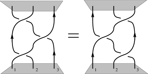
Figure 1.2: Pictorial presentation of the braid relation $\tau_{1}\tau_{2}\tau_{1}=\tau_{2}\tau_{1}\tau_{2}$. The particle trajectories corresponding to the composition of exchanges $\tau_{1}\tau_{2}\tau_{1}$ (diagram at the l.h.s.) can be continuously deformed into the trajectories associated with the composition of exchanges $\tau_{2}\tau_{1}\tau_{2}$ (r.h.s. diagram).

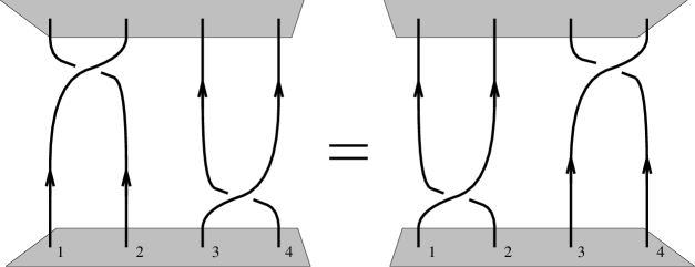
Figure 1.3: The braid relation $\tau_{1}\tau_{3}=\tau_{3}\tau_{1}$ expresses the fact that the particle trajectories displayed in the l.h.s. diagram can be continuously deformed into the trajectories in the r.h.s. diagram.

The one dimensional UIR’s of the braid group $B_{n}({\mbox{\bf R}}^{2})$ are labeled by an angular parameter $\Theta\in[0,2\pi)$ and are defined by assigning the same phase factor to all generators. That is,

$$\tau_{i} \mapsto \exp(\imath\Theta),$$ (1.2.5)

for all $i\in 1,\ldots,n-1$. The quantization of a system of $n$ identical particles in the plane corresponding to an arbitrary but fixed $\Theta\in[0,2\pi)$ is then given by a multi-valued (scalar) wave function that generates the quantum statistical phase $\exp(\imath\Theta)$ upon a counterclockwise interchange of two adjacent particles. For $\Theta=0$ and $\Theta=\pi$, we are dealing with bosons and fermions respectively. The particle species related to other values of $\Theta$ have been called anyons [131]. Quantum statistics deviating from conventional permutation statistics is known under various names in the literature, e.g. fractional statistics, anyon statistics and exotic statistics. We adopt the following nomenclature. An identical particle system described by a (multi-valued) wave function that transforms as an one dimensional (abelian) UIR of the braid group $B_{n}({\mbox{\bf R}}^{2})$ ($\Theta\neq 0,\pi$) is said to realize abelian braid statistics. If an identical particle system is described by a multi-component wave function carrying an higher dimensional UIR of the braid group, then the particles are said to obey nonabelian braid statistics.

Figure 1.4: The monodromy operator $\gamma_{ij}$ takes particle $i$ counterclockwise around particle $j$.

A system of $n$ distinguishable particles moving in the plane, in turn, is described by the non-simply connected configuration space

$${\cal Q}_{n}({\mbox{\bf R}}^{2}) = ({\mbox{\bf R}}^{2})^{n}-D.$$ (1.2.6)

The fundamental group of this configuration space is the so-called colored braid group $P_{n}({\mbox{\bf R}}^{2})$, also known as the pure braid group. The colored braid group $P_{n}({\mbox{\bf R}}^{2})$ is the subgroup of the ordinary braid group $B_{n}({\mbox{\bf R}}^{2})$ generated by the monodromy operators

$$\gamma_{ij} := \tau_{i}\cdots\tau_{j-2}\tau_{j-1}^{2}\tau_{j-2}^{-1}\cdots\tau_{i}^{-1}\qquad\qquad\mbox{with}\;1\leq i<j\leq n.$$ (1.2.7)

Here, the $\tau_{i}$’s are the generators of $B_{n}({\mbox{\bf R}}^{2})$ acting on the set of $n$ numbered distinguishable particles as displayed in figure 1.1. It then follows from the definition (1.2.7) that the monodromy operator $\gamma_{ij}$ takes particle $i$ counterclockwise around particle $j$ as depicted in figure 1.4. The different UIR’s of $P_{n}({\mbox{\bf R}}^{2})$ now label the inequivalent ways to quantize a system of $n$ distinguishable particles in the plane. Finally, a planar system that consists of a subsystem of identical particles of one type, a subsystem of identical particles of another type and so on, is of course also conceivable. The fundamental group of the configuration space of such a system is known as a partially colored braid group. Let the total number of particles of this system again be $n$, then the associated partially colored braid group is the subgroup of the ordinary braid group $B_{n}({\mbox{\bf R}}^{2})$ generated by the braid operators that interchange identical particles and the monodromy operators acting on distinguishable particles. See for example [32, 33].

To conclude, the fundamental excitations in planar discrete gauge theories, namely magnetic vortices and matter charges, are in principle bosons. As will be argued in the next sections, in the first quantized description, these particles acquire braid statistics through the Aharonov-Bohm effect. Hence, depending on whether we are dealing with a system of identical particles, a system of distinguishable particles or a mixture, the associated multi-particle wave function transforms as an representation of the ordinary braid group, colored braid group or partially colored braid group respectively.

1.3 ${\mbox{\bf Z}}_{N}$ gauge theory

The simplest example of a broken gauge theory is an $U(1)$ gauge theory broken down to the cyclic subgroup ${\mbox{\bf Z}}_{N}$. This symmetry breaking scheme occurs in an abelian Higgs model in which the field that condenses carries charge $Ne$, with $e$ the fundamental charge unit [82]. The case $N=2$ is in fact realized in the ordinary BCS superconductor, as the field that condenses in the BCS superconductor is that associated with the Cooper pair carrying charge $2e$.

This section is devoted to a discussion of such an abelian Higgs model focussing on the ${\mbox{\bf Z}}_{N}$ gauge theory describing the long range physics. The outline is as follows. In section 1.3.1, we will start with a brief review of the screening mechanism for the electromagnetic fields of external matter charges $q$ in the Higgs phase. We will argue that the external matter charges, which are multiples of the fundamental charge $e$ rather then multiples of the Higgs charge $Ne$, are surrounded by screening charges provided by the Higgs condensate. These screening charges screen the electromagnetic fields around the external charges. Thus no long range Coulomb interactions persist among the external charges. The main point of section 1.3.2 will be, however, that the screening charges do not screen the Aharonov-Bohm interactions between the external charges and the magnetic vortices, which also occur in these models. As a consequence, long range Aharonov-Bohm interactions persist between the vortices and the external matter charges in the Higgs phase. Upon circumnavigating a magnetic vortex (carrying a flux $\phi$ which is a multiple of the fundamental flux unit $\frac{2\pi}{Ne}$ in this case) with an external charge $q$ (being a multiple of the fundamental charge unit $e$) the wave function of the system picks up the Aharonov-Bohm phase $\exp(\imath q\phi)$. These Aharonov-Bohm phases lead to observable low energy scattering effects from which we conclude that the physically distinct superselection sectors in the Higgs phase can be labeled as $(a,n)$, where $a$ stands for the number of fundamental flux units $\frac{2\pi}{Ne}$ and $n$ for the number of fundamental charge units $e$. In other words, the spectrum of the ${\mbox{\bf Z}}_{N}$ gauge theory in the Higgs phase consists of pure charges $n$, pure fluxes $a$ and dyonic combinations. Given the remaining long range Aharonov-Bohm interactions, these charge and flux quantum numbers are defined modulo $N$. Having identified the spectrum and the long range interactions as the topological Aharonov-Bohm effect, we proceed with a closer examination of this ${\mbox{\bf Z}}_{N}$ gauge theory in section 1.3.3. It will be argued that multi-particle systems in general satisfy abelian braid statistics, that is, the wave functions realize one dimensional representations of the associated braid group. In particular, identical dyons behave as anyons. We will also discuss the composition rules for the charge/flux quantum numbers when two particles are brought together. A key result of this section is a topological proof of the spin-statistics connection for the particles in the spectrum. This proof is of a general nature and applies to all the theories that will be discussed in this thesis.

1.3.1 Coulomb screening

Let us start by emphasizing that we will work in 2+1 dimensional Minkowski space. The abelian Higgs model in which we are interested is given by

$$S = \int d\,^{3}x\;({\cal L}_{\mbox{\scriptsize YMH}}+{\cal L}_{\mbox{\scriptsize matter}})$$ (1.3.1)

$${\cal L}_{\mbox{\scriptsize YMH}} = -\frac{1}{4}F^{\kappa\nu}F_{\kappa\nu}+({\cal D}^{\kappa}\Phi)^{*}{\cal D}_{\kappa}\Phi-V(|\Phi|)$$ (1.3.2)

$${\cal L}_{\mbox{\scriptsize matter}} = -j^{\kappa}A_{\kappa},$$ (1.3.3)

where the Higgs field $\Phi$ is assumed to carry the charge $Ne$ w.r.t. the compact $U(1)$ gauge symmetry. In the conventions we will adopt, this means that the covariant derivative reads ${\cal D}_{\rho}\Phi=(\partial_{\rho}+\imath NeA_{\rho})\Phi$. Furthermore, the potential

$$V(|\Phi|) = \frac{\lambda}{4}(|\Phi|^{2}-v^{2})^{2}\qquad\qquad\lambda,v>0,$$ (1.3.4)

endows the Higgs field with a nonvanishing vacuum expectation value $|\langle\Phi\rangle|=v$, which implies that the the global continuous $U(1)$ symmetry is spontaneously broken. In this particular model the symmetry is not completely broken, however. Under global symmetry transformations $\Lambda(\alpha)$, with $\alpha\in[0,2\pi)$ being the $U(1)$ parameter, the ground states transform as

$$\Lambda(\alpha)\langle\Phi\rangle = e^{\imath N\alpha}\langle\Phi\rangle,$$ (1.3.5)

since the Higgs field was assumed to carry the charge $Ne$. Clearly, the residual symmetry group of the ground states is the finite cyclic group ${\mbox{\bf Z}}_{N}$ corresponding to the elements $\alpha=2\pi k/N$ with $k\in 0,1,\ldots,N-1$.

To proceed, the field equations following from variation of the action (1.3.1) w.r.t. the vector potential $A_{\kappa}$ and the Higgs field $\Phi$ are simply inferred as

$$\partial_{\nu}F^{\nu\kappa} = j^{\kappa}+j^{\kappa}_{H}$$ (1.3.6)

$${\cal D}_{\kappa}{\cal D}^{\kappa}\Phi^{*} = -\frac{\partial V}{\partial\Phi},$$ (1.3.7)

where

$$j^{\kappa}_{H} = \imath Ne(\Phi^{*}{\cal D}^{\kappa}\Phi-({\cal D}^{\kappa}\Phi)^{*}\Phi),$$ (1.3.8)

denotes the Higgs current.

In this section, we will only be concerned with the Higgs screening mechanism for the electromagnetic fields of the matter charges, which are provided by the conserved matter current $j^{\kappa}$ in (1.3.3). For convenience, we discard the dynamics of the fields that are associated with this current and simply treat $j^{\kappa}$ as being external. In fact, for our purposes the only important feature of the current $j^{\kappa}$ is that it allows us to introduce global $U(1)$ charges $q$ in the Higgs phase, which are multiples of the fundamental charge $e$ rather then multiples of the Higgs charge $Ne$, so that all conceivable charge sectors can be discussed.

Let us start by recalling some of the basic dynamical features of this model. First of all, the complex Higgs field

$$\Phi(x) = \rho(x)\exp(\imath\sigma(x)),$$ (1.3.9)

describes two physical degrees of freedom: the charged Goldstone boson field $\sigma(x)$ and the physical field $\rho(x)-v$ with mass $M_{H}=v\sqrt{2\lambda}$ corresponding to the charged neutral Higgs particles. The Higgs mass $M_{H}$ sets the characteristic energy scale of this model. At energies larger then $M_{H}$, the massive Higgs particles can be excited. At energies smaller then $M_{H}$ on the other hand, the massive Higgs particles can not be excited. For simplicity we will restrict ourselves to the latter low energy regime. In this case, the Higgs field is completely condensed, i.e. it acquires ground state values everywhere

$$\Phi(x) \longmapsto \langle\Phi(x)\rangle=v\exp(\imath\sigma(x)).$$ (1.3.10)

The condensation of the Higgs field implies that the Higgs model in the low energy regime is governed by the effective action obtained from the action (1.3.1) by the following simplification

$${\cal L}_{\mbox{\scriptsize YMH}} \longmapsto -\frac{1}{4}F^{\kappa\nu}F_{\kappa\nu}+\frac{M_{A}^{2}}{2}\tilde{A}^{\kappa}\tilde{A}_{\kappa}$$ (1.3.11)

$$\tilde{A}_{\kappa} := A_{\kappa}+\frac{1}{Ne}\partial_{\kappa}\sigma$$ (1.3.12)

$$M_{A} := Nev\sqrt{2}.$$ (1.3.13)

In other words, the dynamics of the Higgs medium arising here is described by the effective field equations inferred from varying the effective action w.r.t. the gauge field $A_{\kappa}$ and the Goldstone boson $\sigma$ respectively

$$\partial_{\nu}F^{\nu\kappa} = j^{\kappa}+j^{\kappa}_{\mbox{\scriptsize scr}}$$ (1.3.14)

$$\partial_{\kappa}j^{\kappa}_{\mbox{\scriptsize scr}} = 0,$$ (1.3.15)

with

$$j^{\kappa}_{\mbox{\scriptsize scr}} = -M_{A}^{2}\tilde{A}^{\kappa},$$ (1.3.16)

the simple form the Higgs current (1.3.8) takes in the low energy regime.

It is easily verified that the field equations (1.3.14) and (1.3.15) can be cast in the following form

$$(\partial_{\nu}\partial^{\nu}+M_{A}^{2})\tilde{A}^{\kappa} = j^{\kappa}$$ (1.3.17)

$$\partial_{\kappa}\tilde{A}^{\kappa} = 0,$$ (1.3.18)

which clearly indicates that the gauge invariant vector field $\tilde{A}_{\kappa}$ has become massive. More specifically, in this 2+1 dimensional setting it describes two physical degrees of freedom both carrying the same mass $M_{A}$ defined in (1.3.13). Consequently, the electromagnetic fields around sources in the Higgs medium decay exponentially with mass $M_{A}$. Of course, the number of degrees of freedom is conserved. We started with an unbroken theory with two physical degrees of freedom $\rho-v$ and $\sigma$ for the Higgs field and one for the massless gauge field $A_{\kappa}$. After spontaneous symmetry breaking the Goldstone boson $\sigma$ conspires with the gauge field $A_{\kappa}$ to form a massive vector field $\tilde{A}_{\kappa}$ with two degrees of freedom, while the real scalar field $\rho$ decouples in the low energy regime.

Let us finally turn to the response of the Higgs medium to the external point charges $q=ne$ introduced by the matter current $j^{\kappa}$ in (1.3.3). From (1.3.17), we infer that the gauge invariant combined field $\tilde{A}_{\kappa}$ around this current drops off exponentially with mass $M_{A}$. Thus the gauge field $A_{\kappa}$ necessarily becomes pure gauge at distances much larger then $1/M_{A}$ from these point charges, and the electromagnetic fields generated by this current vanish accordingly. In other words, the electromagnetic fields generated by the external charges $q$ are completely screened by the Higgs medium. From the field equations (1.3.14) and (1.3.15) it is clear how the Higgs screening mechanism works. The external matter current $j^{\kappa}$ induces a screening current (1.3.16) in the Higgs medium proportional to the vector field $\tilde{A}_{\kappa}$. This becomes most transparent upon considering Gauss’ law in this case

$$Q\;=\;\int d\,^{2}x\;\nabla\cdot{\mbox{\bf E}}\;=\;q+q_{\mbox{\scriptsize scr}}\;=\;0,$$ (1.3.19)

which shows that the external point charge $q$ is surrounded by a cloud of screening charge density $j^{0}_{\mbox{\scriptsize scr}}$ with support of characteristic size $1/M_{A}$. The contribution of the screening charge $q_{\mbox{\scriptsize scr}}=\int d\,^{2}x\,j^{0}_{\mbox{\scriptsize scr}}=-q$ to the long range Coulomb fields completely cancels the contribution of the external charge $q$. Thus we arrive at the well-known result that long range Coulomb interactions between external charges vanish in the Higgs phase.

It has long been believed that with the vanishing of the Coulomb interactions, there are no long range interactions left for the external charges in the Higgs phase. However, it was indicated by Krauss, Wilczek and Preskill [82, 107] that this is not the case. They noted that when the $U(1)$ gauge group is not completely broken, but instead we are left with a finite cyclic manifest gauge group ${\mbox{\bf Z}}_{N}$ in the Higgs phase, the external charges may still have long range Aharonov-Bohm interactions with the magnetic vortices also appearing in this model. These interactions are of a purely quantum mechanical nature with no classical analogue. The physical mechanism behind the survival of Aharonov-Bohm interactions was subsequently uncovered in [21]: the screening charges $q_{\mbox{\scriptsize scr}}$ only couple to the Coulomb interactions and not to the Aharonov-Bohm interactions. As a result, the screening charges only screen the long range Coulomb interactions among the external charges, but not the aforementioned long range Aharonov-Bohm interactions with the magnetic fluxes. We will discuss this phenomenon in further detail in the next section.

1.3.2 Survival of the Aharonov-Bohm effect

A distinguishing feature of the abelian Higgs model (1.3.2) is that it supports stable vortices carrying magnetic flux [1, 99]. These are static classical solutions of the field equations with finite energy and correspond to topological defects in the Higgs condensate, which are pointlike in this 2+1 dimensional setting. Here, we will briefly review the basic properties of these magnetic vortices and subsequently elaborate on their long range Aharonov-Bohm interactions with the screened external charges.

The energy density following from the action (1.3.2) for time independent field configurations reads

$${\cal E} = \frac{1}{2}(E^{i}E^{i}+B^{2})+(NeA_{0})^{2}|\Phi|^{2}+{\cal D}_{i}\Phi({\cal D}_{i}\Phi)^{*}+V(|\Phi|).$$ (1.3.20)

All the terms occurring here are obviously positive definite. For field configurations of finite energy these terms should therefore vanish separately at spatial infinity. The potential (1.3.4) vanishes for ground states only. Thus the Higgs field is necessarily condensed (1.3.10) at spatial infinity. Of course, the Higgs condensate can still make a nontrivial winding in the manifold of ground states. Such a winding at spatial infinity corresponds to a nontrivial holonomy in the Goldstone boson field

$$\sigma(\theta+2\pi)-\sigma(\theta) = 2\pi a,$$ (1.3.21)

where $a$ is required to be an integer in order to leave the Higgs condensate (1.3.10) itself single valued, while $\theta$ denotes the polar angle. Requiring the fourth term in (1.3.20) to be integrable translates into the condition

$${\cal D}_{i}\Phi(r\rightarrow\infty)\sim\tilde{A}_{i}(r\rightarrow\infty)=0,$$ (1.3.22)

with $\tilde{A}_{i}$ the gauge invariant combination of the Goldstone boson and the gauge field defined in (1.3.12). Consequently, the nontrivial holonomy in the Goldstone boson field has to be compensated by an holonomy in the gauge fields and the vortices carry magnetic flux $\phi$ quantized as

$$\phi\;=\;\oint dl^{i}A^{i}\;=\;\frac{1}{Ne}\oint dl^{i}\partial_{i}\sigma\;=\;\frac{2\pi a}{Ne}\qquad\mbox{with $a\in{\mbox{\bf Z}}$.}$$ (1.3.23)

To proceed, the third term in the energy density (1.3.20) disappears at spatial infinity if and only if $A_{0}(r\rightarrow\infty)=0$, and all in all we see that the gauge field $A_{\kappa}$ is pure gauge at spatial infinity, so the first two terms vanish automatically. To end up with a regular field configuration corresponding to a nontrivial winding (1.3.21) of the Higgs condensate at spatial infinity, the Higgs field $\Phi$ should obviously become zero somewhere in the plane. Thus the Higgs phase is necessarily destroyed in some finite region in the plane. A closer evaluation of the energy density (1.3.20) shows that the Higgs field grows monotonically from its zero value to its asymptotic ground state value (1.3.10) at the distance $1/M_{H}$, the so-called core size [1, 99]. Outside the core we are in the Higgs phase, and the physics is described by the effective Lagrangian (1.3.11), while inside the core the $U(1)$ symmetry is restored. The magnetic field associated with the flux (1.3.23) of the vortex reaches its maximum inside the core where the gauge fields are massless. Outside the core the gauge fields become massive and the magnetic field drops off exponentially with the mass $M_{A}$. The core size $1/M_{H}$ and the penetration depth $1/M_{A}$ of the magnetic field are the two length scales characterizing the magnetic vortex. The formation of magnetic vortices depends on the ratio of these two scales. An evaluation of the free energy (see for instance [62]) yields that magnetic vortices can be formed iff $M_{H}/M_{A}=\sqrt{\lambda}/Ne\geq 1$. We will always assume that this inequality is satisfied, so that magnetic vortices may indeed appear in the Higgs medium. In other words, we assume that we are dealing with a superconductor of type II.

We now have two dually charged types of sources in the Higgs medium. On the one hand there are the vortices $\phi$ being sources for screened magnetic fields, and on the other hand the external charges $q$ being sources for screened electric fields. The magnetic fields of the vortices are localized within regions of length scale $1/M_{H}$ dropping off with mass $M_{A}$ at larger distances. The external charges are point particles with Coulomb fields completely screened at distances $>1/M_{A}$. Henceforth, we will restrict our considerations to the low energy regime (or alternatively send the Higgs mass $M_{H}$ and the mass $M_{A}$ of the gauge field to infinity by sending the symmetry breaking scale to infinity). This means that the distances between the sources remain much larger then the Higgs length scale $1/M_{H}$. In other words, the electromagnetic fields associated with the magnetic- and electric sources never overlap and the Coulomb interactions between these sources vanish in the low energy regime. Thus from a classical point of view there are no long range interactions left between the sources. From a quantum mechanical perspective, however, it is known that in ordinary electromagnetism shielded localized magnetic fluxes can affect electric charges even though their mutual electromagnetic fields do not interfere. When an electric charge $q$ encircles a localized magnetic flux $\phi$, it notices the nontrivial holonomy in the locally flat gauge fields around the flux and in this process the wave function picks up a quantum phase $\exp(\imath q\phi)$ in the first quantized description. This is the celebrated Aharonov-Bohm effect [4], which is a purely quantum mechanical effect with no classical analogue. These long range Aharonov-Bohm interactions are of a topological nature, i.e. as long as the charge never enters the region where the flux is localized, the Aharonov-Bohm interactions only depend on the number of windings of the charge around the flux and not on the distance between the charge and the flux. Due to a remarkable cancellation in the effective action (1.3.11), the screening charges $q_{\mbox{\scriptsize scr}}$ accompanying the external charges do not exhibit the Aharonov-Bohm effect. As a result the long range Aharonov-Bohm effect persists between the external charges $q$ and the magnetic vortices $\phi$ in the Higgs phase. We will argue this in further detail.

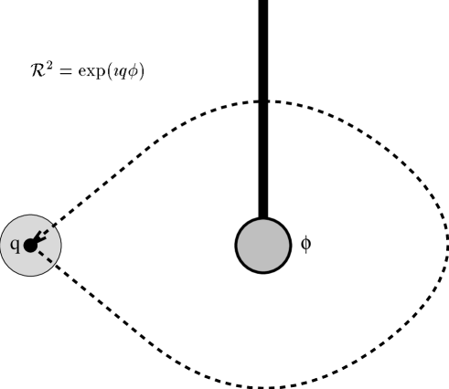
Figure 1.5: Taking a screened external charge $q$ around a magnetic vortex $\phi$ in the Higgs medium generates the Aharonov-Bohm phase $\exp(\imath q\phi)$. We have emphasized the extended structure of these sources, although this structure will not be probed in the low energy regime to which we confine ourselves here. The shaded region around the external point charge $q$ represents the cloud of screening charge of characteristic size $1/M_{A}$. The flux of the vortex is confined to the shaded circle bounded by the core at the distance $1/M_{H}$ from its centre. The string attached to the core represents the Dirac string of the flux, i.e. the strip in which the nontrivial parallel transport in the gauge fields takes place.

Consider the system depicted in figure 1.5 consisting of an external charge $q$ and a magnetic vortex $\phi$ in the Higgs phase well separated from each other. We have depicted these sources as extended objects, but in the low energy regime their extended structure will never be probed and it is legitimate to describe these sources as point particles moving in the plane. The magnetic vortex introduces a nontrivial holonomy (1.3.23) in the gauge fields to which the external charge couples through the matter coupling (1.3.3)

$$-\int\!\!d\,^{2}x\;j^{\kappa}A_{\kappa} = \frac{q\phi}{2\pi}\dot{\chi}_{\phi}({\mbox{\bf y}}(t)-{\mbox{\bf z}}(t)),$$ (1.3.24)

where ${\mbox{\bf y}}(t)$ and ${\mbox{\bf z}}(t)$ respectively denote the worldlines of the external charge $q$ and magnetic vortex $\phi$ in the plane. In the conventions we will use throughout this thesis, the nontrivial parallel transport in the gauge fields around the magnetic vortices takes place in a thin strip (simply called Dirac string from now) attached to the core of the vortex going off to spatial infinity in the direction of the positive vertical axis. This situation can always be reached by a smooth gauge transformation, and simplifies the bookkeeping for the braid processes involving more than two particles. The multi-valued function $\chi_{\phi}({\mbox{\bf x}})$ with support in the aforementioned strip of parallel transport is a direct translation of this convention. It increases from $0$ to $2\pi$ if the strip is passed from right to left. Thus when the external charge $q$ moves through this strip once in the counterclockwise fashion indicated in figure 1.5, the topological interaction Lagrangian (1.3.24) generates the action $q\phi$. In the same process the screening charge $q_{\mbox{\scriptsize scr}}=-q$ accompanying the external charge $q$ also moves through this strip of parallel transport. Since the screening charge has a sign opposite to the sign of the external charge, it seems, at first sight, that the total topological action associated with encircling a flux by a screened external charge vanishes. This is not the case though. The screening charge $q_{\mbox{\scriptsize scr}}$ not only couples to the holonomy in the gauge field $A_{\kappa}$ around the vortex but also to the holonomy in the Goldstone boson field $\sigma$. This follows directly from the effective low energy Lagrangian (1.3.11). Let $j_{\mbox{\scriptsize scr}}^{\kappa}$ be the screening current (1.3.16) associated with the screening charge $q_{\mbox{\scriptsize scr}}$. The interaction term in (1.3.11) couples this current to the massive gauge invariant field $\tilde{A}_{\kappa}$ around the vortex: $-j_{\mbox{\scriptsize scr}}^{\kappa}\tilde{A}_{\kappa}$. As we have seen in (1.3.22), the holonomies in the gauge field and the Goldstone boson field are related at large distances from the core of the vortex, such that $\tilde{A}_{\kappa}$ strictly vanishes. As a consequence, the interaction term $-j_{\mbox{\scriptsize scr}}^{\kappa}\tilde{A}_{\kappa}$ vanishes and indeed the matter coupling (1.3.24) summarizes all the remaining long range interactions in the low energy regime [21].

Being a total time derivative, the topological interaction term (1.3.24) does not appear in the equations of motion and has no effect at the classical level. In the first quantized description however, the appearance of this term has far reaching consequences. This is most easily seen using the path integral method for quantization. In the path integral formalism, the transition amplitude or propagator from one point in the configuration space at some time to another point at some later time, is given by a weighed sum over all the paths connecting the two points. In this sum, the paths are weighed by their action $\exp(\imath S)$. If we apply this prescription to our charge/flux system, we see that the Lagrangian (1.3.24) assigns amplitudes differing by $\exp(\imath q\phi)$ to paths differing by an encircling of the external charge $q$ around the flux $\phi$. Thus nontrivial interference takes place between paths associated with different winding numbers of the charge around the flux. This is the Aharonov-Bohm effect which becomes observable in quantum interference experiments [4], such as low energy scattering experiments of external charges from the magnetic vortices. The cross sections measured in these Aharonov-Bohm scattering experiments can be found in appendix 1.A.

There are two equivalent ways to present the appearance of the Aharonov-Bohm interactions. In the above discussion of the path integral formalism we kept the topological Aharonov-Bohm interactions in the Lagrangian for this otherwise free charge/flux system. In this description we work with single valued wave functions on the configuration space for a given time slice

$$\Psi_{q\phi}({\mbox{\bf y}},{\mbox{\bf z}},t) = \Psi_{q}({\mbox{\bf y}},t)\Psi_{\phi}({\mbox{\bf z}},t)\qquad\qquad\mbox{with ${\mbox{\bf y}}\neq{\mbox{\bf z}}$}.$$ (1.3.25)

The factorization of the wave functions follows because there are no interactions between the external charge and the magnetic flux other then the topological one (1.3.24). The time evolution of these wave functions is given by the propagator associated with the two particle Lagrangian

$$L = \frac{1}{2}m_{q}\dot{{\mbox{\bf y}}}^{2}+\frac{1}{2}m_{\phi}\dot{{\mbox{\bf z}}}^{2}+\frac{q\phi}{2\pi}\dot{\chi}_{\phi}({\mbox{\bf y}}(t)-{\mbox{\bf z}}(t)).$$ (1.3.26)

Equivalently, we may absorb the topological interaction (1.3.24) in the boundary condition of the wave functions and work with multi-valued wave functions

$$\tilde{\Psi}_{q\phi}({\mbox{\bf y}},{\mbox{\bf z}},t) := e^{\imath\frac{q\phi}{2\pi}\chi_{\phi}({\mbox{\scriptsize\bf y}}-{\mbox{\scriptsize\bf z}})}\;\Psi_{q}({\mbox{\bf y}},t)\Psi_{\phi}({\mbox{\bf z}},t),$$ (1.3.27)

which propagate with the completely free two particle Lagrangian [137] (see also [59])

$$\tilde{L} = \frac{1}{2}m_{q}\dot{{\mbox{\bf y}}}^{2}+\frac{1}{2}m_{\phi}\dot{{\mbox{\bf z}}}^{2}.$$ (1.3.28)

We cling to the latter description from now on, that is, we will always absorb the topological interaction terms in the boundary condition of the wave functions. For later use and convenience we set some more conventions. We will adopt a compact Dirac notation emphasizing the internal charge/flux quantum numbers of the particles. In this notation, the quantum state describing a charge or flux localized at some position x in the plane is presented as

$$|{\mbox{charge/flux}}\rangle:=|{\mbox{charge/flux}},{\mbox{\bf x}}\rangle=|{\mbox{charge/flux}}\rangle|{\mbox{\bf x}}\rangle.$$ (1.3.29)

To proceed, the charges $q=ne$ will be abbreviated by the number $n$ of fundamental charge units $e$ and the fluxes $\phi$ by the number $a$ of fundamental flux units $\frac{2\pi}{Ne}$. With the two particle quantum state $|n\rangle|a\rangle$ we then indicate the multi-valued wave function

$$|n\rangle|a\rangle := e^{\imath\frac{na}{N}\chi_{a}({\mbox{\scriptsize\bf x}}-{\mbox{\scriptsize\bf y}})}\;|n,{\mbox{\bf x}}\rangle|a,{\mbox{\bf y}}\rangle,$$ (1.3.30)

where by convention the particle that is located most left in the plane (in this case the external charge $q=ne$), appears most left in the tensor product. The process of transporting the charge adiabatically around the flux in a counterclockwise fashion as depicted in figure 1.5 is now summarized by the action of the monodromy operator on this two particle state

$${\cal R}^{2}\;|n\rangle|a\rangle = e^{\frac{2\pi\imath}{N}na}\;|n\rangle|a\rangle,$$ (1.3.31)

which boils down to a residual global ${\mbox{\bf Z}}_{N}$ transformation by the flux $a$ of the vortex on the charge $n$.

Given the residual long range Aharonov-Bohm interactions (1.3.31) in the Higgs phase, the labeling of the charges and the fluxes by integers is of course highly redundant. Charges $n$ differing by a multiple of $N$ can not be distinguished. The same holds for the fluxes $a$. Thus the charge and flux quantum numbers are defined modulo $N$ in the residual manifest ${\mbox{\bf Z}}_{N}$ gauge theory arising in the Higgs phase. Besides these pure ${\mbox{\bf Z}}_{N}$ charges and fluxes the full spectrum consists of charge/flux composites or dyons produced by fusing the charges and fluxes. We return to a detailed discussion of this spectrum and the topological interactions it exhibits in the next section.

Let us recapitulate our results from a more conceptual point of view (see also [9, 107, 89] in this connection). In unbroken (compact) quantum electrodynamics the quantized matter charges $q=ne$ (with $n\in{\mbox{\bf Z}}$), corresponding to the different unitary irreducible representations (UIR’s) of the global symmetry group $U(1)$, carry long range Coulomb fields. In other words, the Hilbert space of this theory decomposes into a direct sum of orthogonal charge superselection sectors that can be distinguished by measuring the associated Coulomb fields at spatial infinity. Local observables preserve this decomposition, since they can not affect these long range properties of the charges. The charge sectors can alternatively be distinguished by their response to global $U(1)$ transformations, since these are related to physical measurements of the Coulomb fields at spatial infinity through Gauss’ law. Let us emphasize that the states in the Hilbert space are of course invariant under local gauge transformations, i.e. gauge transformations with finite support, which become trivial at spatial infinity.

Here we touch upon the important distinction between global symmetry transformations and local gauge transformations. Although both leave the action of the model invariant, their physical meaning is rather different. A global symmetry (independent of the coordinates) is a true symmetry of the theory and in particular leads to a conserved Noether current. Local gauge transformations, on the other hand, correspond to a redundancy in the variables describing this model and should therefore be modded out in the construction of the physical Hilbert space. In the $U(1)$ gauge theory under consideration the fields that transform nontrivially under the global $U(1)$ symmetry are the matter fields. The associated Noether current $j^{\kappa}$ shows up in the Maxwell equations. More specifically, the conserved Noether charge $q=\int d\,^{2}x\,j^{0}$, being the generator of the global symmetry, is identified with the Coulomb charge $Q=\int d\,^{2}x\,\nabla\cdot{\mbox{\bf E}}$ through Gauss’ law. This is the aforementioned relation between the global symmetry transformations and physical Coulomb charge measurements at spatial infinity.

Although the long range Coulomb fields vanish when this $U(1)$ gauge theory is spontaneously broken down to a finite cyclic group ${\mbox{\bf Z}}_{N}$, we are still able to detect ${\mbox{\bf Z}}_{N}$ charge at arbitrary long distances through the Aharonov-Bohm effect. In other words, there remains a relation between residual global symmetry transformations and physical charge measurements at spatial infinity. The point is that we are left with a gauged ${\mbox{\bf Z}}_{N}$ symmetry in the Higgs phase, as witnessed by the appearance of stable magnetic fluxes in the spectrum. The magnetic fluxes introduce holonomies in the (locally flat) gauge fields, which take values in the residual manifest gauge group ${\mbox{\bf Z}}_{N}$ to leave the Higgs condensate single valued. To be specific, the holonomy of a given flux is classified by the group element picked up by the Wilson loop operator

$$W({\cal C},{\mbox{\bf x}}_{0}) = P\exp\,(\imath e\oint A^{i}dl^{i})\;\in{\mbox{\bf Z}}_{N},$$ (1.3.32)

where ${\cal C}$ denotes a loop enclosing the flux starting and ending at some fixed base point ${\mbox{\bf x}}_{0}$ at spatial infinity. The path ordering indicated by $P$ is trivial in this abelian case. These fluxes can be used for charge measurements in the Higgs phase by means of the Aharonov-Bohm effect (1.3.31). This purely quantum mechanical effect, boiling down to a global ${\mbox{\bf Z}}_{N}$ gauge transformation on the charge by the group element (1.3.32), is topological. It persists at arbitrary long ranges and therefore distinguishes the nontrivial ${\mbox{\bf Z}}_{N}$ charge sectors in the Higgs phase. Thus the result of the Higgs mechanism for the charge sectors can be summarized as follows: the charge superselection sectors of the original $U(1)$ gauge theory, which were in one-to-one correspondence with the UIR’s of the global symmetry group $U(1)$, branch to UIR’s of the residual (gauged) symmetry group ${\mbox{\bf Z}}_{N}$ in the Higgs phase.

An important conclusion from this discussion is that a spontaneously broken $U(1)$ gauge theory in general can have distinct Higgs phases corresponding to different manifest gauge groups ${\mbox{\bf Z}}_{N}$. The simplest example is a $U(1)$ gauge theory with two Higgs fields; one carrying a charge $Ne$ and the other a charge $e$. There are in principle two possible Higgs phases in this particular theory, depending on whether the ${\mbox{\bf Z}}_{N}$ gauge symmetry remains manifest or not. In the first case only the Higgs field with charge $Ne$ is condensed and we are left with nontrivial ${\mbox{\bf Z}}_{N}$ charge sectors. In the second case the Higgs field carrying the fundamental charge $e$ is condensed. No charge sectors survive in this completely broken phase. These two Higgs phases, separated by a phase transition, can clearly be distinguished by probing the existence of ${\mbox{\bf Z}}_{N}$ charge sectors. This is exactly the content of the nonlocal order parameter constructed by Preskill and Krauss [107] (see also [9, 10, 11, 90, 91] in this context). In contrast with the Wilson loop operator and the ’t Hooft loop operator distinguishing the Higgs and confining phase of a given gauge theory through the dynamics of electric and magnetic flux tubes [69, 133], this order parameter is of a topological nature. To be specific, in this 2+1 dimensional setting it amounts to evaluating the expectation value of a closed electric flux tube linked with a closed magnetic flux loop corresponding to the worldlines of a minimal ${\mbox{\bf Z}}_{N}$ charge/anti-charge pair linked with the worldlines of a minimal ${\mbox{\bf Z}}_{N}$ magnetic flux/anti-flux pair. If the ${\mbox{\bf Z}}_{N}$ gauge symmetry is manifest, this order parameter gives rise to the Aharonov-Bohm phase (1.3.31), whereas it becomes trivial in the completely broken phase with minimal stable flux $\frac{2\pi}{e}$.

1.3.3 Braid and fusion properties of the spectrum

We proceed with a more thorough discussion of the topological interactions described by the residual ${\mbox{\bf Z}}_{N}$ gauge theory in the Higgs phase of the model (1.3.1). As we have argued in the previous section, the complete spectrum of this discrete gauge theory consists of pure ${\mbox{\bf Z}}_{N}$ charges labeled by $n$, pure ${\mbox{\bf Z}}_{N}$ fluxes labeled by $a$ and dyons produced by fusing these charges and fluxes

$$|a\rangle\times|n\rangle = |a,n\rangle\qquad\qquad\mbox{with}\qquad a,n\in 0,1,\ldots,N-1.$$ (1.3.33)

We have depicted this spectrum for a ${\mbox{\bf Z}}_{4}$ gauge theory in figure 1.6.

Figure 1.6: The spectrum of a Higgs phase with residual manifest gauge group ${\mbox{\bf Z}}_{4}$ compactifies to the particles inside the dashed box. The particles outside the box are identified with the ones inside by means of modulo $4$ calculus along the charge and flux axes. The modulo $4$ calculus for the fluxes corresponds to Dirac monopoles/instantons, if these are present. The minimal monopole tunnels the encircled flux into the vacuum.

The topological interactions in these models are completely governed by the Aharonov-Bohm effect (1.3.31) and can simply be summarized as follows

$${\cal R}^{2}\;|a,n\rangle|a^{\prime},n^{\prime}\rangle = e^{\frac{2\pi\imath}{N}(na^{\prime}+n^{\prime}a)}\;|a,n\rangle|a^{\prime},n^{\prime}\rangle$$ (1.3.34)

$${\cal R}\;|a,n\rangle|a,n\rangle = e^{\frac{2\pi\imath}{N}na}\;|a,n\rangle|a,n\rangle$$ (1.3.35)

$$|a,n\rangle\times|a^{\prime},n^{\prime}\rangle = |[a+a^{\prime}],[n+n^{\prime}]\rangle$$ (1.3.36)

$${\cal C}\,|a,n\rangle = |[-a],[-n]\rangle$$ (1.3.37)

$$T\,|a,n\rangle = e^{\frac{2\pi\imath}{N}na}\;|a,n\rangle.$$ (1.3.38)

The expressions (1.3.34) and (1.3.35) sum up the braid properties of the particles in the spectrum (1.3.33). These realize abelian representations of the braid groups discussed in section 1.2. For distinguishable particles only the monodromies, as contained in the pure braid groups (1.2.7), are relevant. In the present context, particles carrying different charge and magnetic flux are distinguishable. When a particular particle $|a,n\rangle$ located at some position in the plane is adiabatically transported around another remote particle $|a^{\prime},n^{\prime}\rangle$ in the counterclockwise fashion depicted in figure 1.4, the total multi-valued wave function picks up the Aharonov-Bohm phase displayed in (1.3.34). In this process, the charge $n$ of the first particle moves through the Dirac string attached to the flux $a^{\prime}$ of the second particle, while the charge $n^{\prime}$ of the second particle moves through the Dirac string of the flux $a$ of the first particle. In short, the total Aharonov-Bohm effect for this monodromy is the composition of a global ${\mbox{\bf Z}}_{N}$ symmetry transformation on the charge $n$ by the flux $a^{\prime}$ and a global transformation on the charge $n^{\prime}$ by the flux $a$. We confined ourselves to the case of two particles so far. The generalization to systems containing more then two particles is straightforward. The quantum states describing these systems are tensor products of localized single particle states $|a,n,{\mbox{\bf x}}\rangle$, where we cling to the convention that the particle that appears most left in the plane appears most left in the tensor product. These multi-valued wave functions carry abelian representations of the colored braid group: the action of the monodromy generators (1.2.7) on these wave functions boils down to the quantum phase in expression (1.3.34).

For identical particles, i.e. particles carrying the same charge and flux, the braid operation depicted in figure 1.1 becomes meaningful. In this braid process, in which two adjacent identical particles $|a,n\rangle$ located at different positions in the plane are exchanged in a counterclockwise way, the charge of the particle that moves ‘behind’ the other dyon encounters the Dirac string attached to the flux of the latter. The result of this exchange in the multi-valued wave function is the quantum statistical phase factor (see expression (1.2.5)) presented in (1.3.35). In other words, the dyons in the spectrum of this ${\mbox{\bf Z}}_{N}$ theory are anyons. In fact, these charge/flux composites are very close to Wilczek’s original proposal for anyons [130].

An important aspect of this theory is that the particles in the spectrum (1.3.33) satisfy the canonical spin-statistics connection. The proof of this connection is of a topological nature and applies in general to all the models that will be considered in this thesis. The fusion rules play a role in this proof and we will discuss these first.

Fusion and braiding are intimately related. Bringing two particles together is essentially a local process. As such, it can never affect global properties. Thus the single particle state that arises after fusion should exhibit the same global properties as the two particle state we started with. In this topological theory, the global properties of a given configuration are determined by its braid properties with the different particles in the spectrum (1.3.33). We have already established that the charges and fluxes become ${\mbox{\bf Z}}_{N}$ quantum numbers under these braid properties. Therefore the complete set of fusion rules, determining the way the charges and fluxes of a two particle state compose into the charge and flux of a single particle state when the pair is brought together, can be summarized as (1.3.36). The rectangular brackets denote modulo $N$ calculus such that the sum always lies in the range $0,1,\ldots,N-1$.

It is worthwhile to digress a little on the dynamical mechanism underlying the modulo $N$ calculus compactifying the flux part of the spectrum. This modulo calculus is induced by magnetic monopoles, when these are present. This observation will become important in chapter 2 where we will study the incorporation of Chern-Simons actions in this theory. The presence of magnetic monopoles can be accounted for by assuming that the compact $U(1)$ gauge theory (1.3.1) arises from a spontaneously broken $SO(3)$ gauge theory. The monopoles we obtain in this particular model are the regular ’t Hooft-Polyakov monopoles [67, 105]. Let us, alternatively, assume that we have singular Dirac monopoles [49] in this compact $U(1)$ gauge theory. In three spatial dimensions, these are point particles carrying magnetic charges $g$ quantized as $\frac{2\pi}{e}$. In the present 2+1 dimensional Minkowski setting, they become instantons describing flux tunneling events $|\Delta\phi|=\frac{2\pi}{e}$. As has been shown by Polyakov [106], the presence of these instantons in unbroken $U(1)$ gauge theory has a striking dynamical effect. It leads to linear confinement of electric charge. In the broken version of these theories, in which we are interested, electric charge is screened and the presence of instantons in the Higgs phase merely implies that the magnetic flux (1.3.23) of the vortices is conserved modulo $N$

instanton: $$a\;\mapsto\;a-N.$$ (1.3.39)

In other words, a flux $N$ moving in the plane (or $N$ minimal fluxes for that matter) can disappear by ending on an instanton. The fact that the instantons tunnel between states that can not be distinguished by the braidings in this theory is nothing but the 2+1 dimensional translation of the unobservability of the Dirac string in three spatial dimensions.

We turn to the connection between spin and statistics. There are in principle two approaches to prove this deep relation, both having their own merits. One approach, originally due to Wightman [122], involves the axioms of local relativistic quantum field theory, and leads to the observation that integral spin fields commute, while half integral spin fields anticommute. The topological approach that we will take here was first proposed by Finkelstein and Rubinstein [58]. It does not rely upon the heavy framework of local relativistic quantum field theory and among other things applies to the topological defects considered in this thesis. The original formulation of Finkelstein and Rubinstein was in the 3+1 dimensional context, but it naturally extends to 2+1 dimensional space time as we will discuss now [22, 25]. See also [60, 61] for an algebraic approach.

The crucial ingredient in the topological proof of the spin-statistics connection for a given model is the existence of an anti-particle for every particle in the spectrum, such that the pair can annihilate into the vacuum after fusion. Consider the process depicted at the l.h.s. of the equality sign in figure 1.7. It describes the creation of two separate identical particle/anti-particle pairs from the vacuum, a subsequent exchange of the particles of the two pairs and finally annihilation of the pairs. To keep track of the writhing of the particle trajectories we depict them as ribbons with a white- and a dark side. It is easily verified now that the closed ribbon associated with the process just explained can be continuously deformed into the ribbon at the r.h.s., which corresponds to a rotation of the particle over an angle of $2\pi$ around its own centre. In other words, the effect of interchanging two identical particles in a consistent quantum description should be the same as the effect of rotating one particle over an angle of $2\pi$ around its centre. The effect of this rotation in the wave function is the spin factor $\exp(2\pi\imath s)$ with $s$ the spin of the particle, which in contrast with three spatial dimensions may be any real number in two spatial dimensions. Therefore the result of exchanging the two identical particles necessarily boils down to a quantum statistical phase factor $\exp(\imath\Theta)$ in the wave function being the same as the spin factor

$$\exp(\imath\Theta) = \exp(2\pi\imath s).$$ (1.3.40)

This is the canonical spin-statistics connection. Actually, a further consistency condition can be inferred from this ribbon argument. The writhing in the particle trajectory can be continuously deformed to a writhing with the same orientation in the anti-particle trajectory. Therefore the anti-particle necessarily carries the same spin and statistics as the particle.

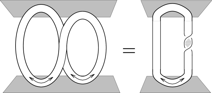
Figure 1.7: Spin-statistics connection. The trajectories describing an exchange of two particles in separate particle/anti-particle pairs (the 8 laying on its back) can be continuously deformed into a single pair in which the particle undergoes a counterclockwise rotation over an angle of $2\pi$ around its own centre (the 0 with a twisted leg).

Sure enough the topological proof of the spin-statistics theorem applies to the ${\mbox{\bf Z}}_{N}$ gauge theory at hand. First of all, we can naturally assign an anti-particle to every particle in the spectrum (1.3.33) through the charge conjugation operator (1.3.37). Under charge conjugation the charge and flux of the particles in the spectrum reverse sign and amalgamating a particle with its charge conjugated partner yields the quantum numbers of the vacuum as follows from the fusion rules (1.3.36). Thus the basic assertion for the above ribbon argument is satisfied. From the quantum statistical phase factor (1.3.35) assigned to the particles and (1.3.40), we then conclude that the particles carry spin. Specifically, under rotation over $2\pi$ the single particle states should give rise to the spin factors displayed in (1.3.38). These spin factors can be interpreted as the Aharonov-Bohm phase generated when the charge of a given dyon rotates around its own flux. Of course, a small separation between the charge and the flux of the dyon is required for this interpretation. Also note that the particles and their anti-particles indeed carry the same spin and statistics, as follows immediately from the invariance of the Aharonov-Bohm effect under charge conjugation.

Having established a complete classification of the topological interactions in these abelian discrete gauge theories, we conclude with some remarks on the Aharonov-Bohm scattering experiments by which these interactions can be probed. (A concise discussion of these purely quantum mechanical experiments can be found in appendix 1.A). It is the monodromy effect (1.3.34) that is measured in these two particle elastic scattering experiments. To be explicit, the symmetric cross section for scattering a particle $|a,n\rangle$ from a particle $|a^{\prime},n^{\prime}\rangle$ is given by

$$\frac{{\rm d}\sigma}{{\rm d}\theta} = \frac{\sin^{2}\left(\frac{\pi}{N}(na^{\prime}+n^{\prime}a)\right)}{2\pi p\sin^{2}(\theta/2)},$$ (1.3.41)

with $p$ the relative momentum of the two particles and $\theta$ the scattering angle. A subtlety arises in scattering experiments involving two identical particles, however. Quantum statistics enters the scene: exchange processes between the scatterer and the projectile have to be taken into account [129, 92]. This leads to the following cross section for Aharonov-Bohm scattering of two identical particles $|a,n\rangle$

$$\frac{{\rm d}\sigma}{{\rm d}\theta} = \frac{\sin^{2}(\frac{2\pi na}{N})}{2\pi p\sin^{2}(\theta/2)}\;+\;\frac{\sin^{2}(\frac{2\pi na}{N})}{2\pi p\cos^{2}(\theta/2)},$$ (1.3.42)

where the second term summarizes the effect of the extra exchange contribution to the direct scattering amplitude.

1.4 Nonabelian discrete gauge theories

The generalization of the foregoing analysis to spontaneously broken models in which we are left with a nonabelian finite gauge group ${H}$ involves essentially new features. In this introductory section, we will establish the complete flux/charge spectrum of such a nonabelian discrete ${H}$ gauge theory and discuss the basic topological interactions among the different flux/charge composites. The outline is as follows. Section 1.4.1 contains a general discussion on the topological classification of stable magnetic vortices and the subtle role magnetic monopoles play in this classification. In section 1.4.2, we subsequently review the properties of the nonabelian magnetic vortices that occur when the residual symmetry group $H$ is nonabelian. The most important one being that these vortices exhibit a nonabelian Aharonov-Bohm effect. To be specific, the fluxes of the vortices, which are labeled by the group elements of ${H}$, affect each other through conjugation when they move around each other [16]. Under the residual global symmetry group ${H}$ the magnetic fluxes transform by conjugation as well, and the conclusion is that the vortices are organized in degenerate multiplets, corresponding to the different conjugacy classes of ${H}$. These classical properties will then be elevated into the first quantized description in which the magnetic vortices are treated as point particles moving in the plane. In section 1.4.3, we finally turn to the matter charges that may occur in these Higgs phases and their Aharonov-Bohm interactions with the magnetic vortices. As has been pointed out in [7, 107], these matter charges are labeled by the different UIR’s $\Gamma$ of the residual global symmetry group ${H}$ and when such a charge encircles a nonabelian vortex it picks up a global symmetry transformation by the matrix $\Gamma(h)$ associated with the flux $h$ of the vortex in the representation $\Gamma$. To conclude, we elaborate on the subtleties involved in the description of dyonic combinations of the nonabelian magnetic fluxes and the matter charges $\Gamma$.

1.4.1 Classification of stable magnetic vortices

Let us start by specifying the spontaneously broken gauge theories in which we are left with a nonabelian discrete gauge theory. In this case, we are dealing with a Higgs field $\Phi$ transforming according to some higher dimensional representation of a continuous nonabelian gauge group ${G}$

$$S_{\mbox{\scriptsize YMH}} = \int d\,^{3}x\;(-\frac{1}{4}F^{a\;\kappa\nu}F_{\kappa\nu}^{a}+({\cal D}^{\kappa}\Phi)^{\dagger}\cdot{\cal D}_{\kappa}\Phi-V(\Phi)),$$ (1.4.1)

and a potential $V(\Phi)$ giving rise to a degenerate set of ground states $\langle\Phi\rangle\neq 0$, which are only invariant under the action of a finite nonabelian subgroup ${H}$ of ${G}$. For simplicity, we make two assumptions. First of all, we assume that this Higgs potential is normalized such that $V(\Phi)\geq 0$ and equals zero for the ground states $\langle\Phi\rangle$. More importantly, we assume that all ground states can be reached from any given one by global ${G}$ transformations. This last assumption implies that the ground state manifold becomes isomorphic to the coset ${G}/{H}$. (Renormalizable examples of potentials doing the job for ${G}\simeq SO(3)$ and ${H}$ some of its point groups can be found in [100]). In the following, we will only be concerned with the low energy regime of this theory, so that the massive gauge bosons can be ignored.

The stable vortices that can be formed in this spontaneously broken gauge theory correspond to noncontractible maps from the circle at spatial infinity (starting and ending at a fixed base point ${\mbox{\bf x}}_{0}$) into the ground state manifold ${G}/{H}$. Different vortices are related to noncontractible maps that can not be continuously deformed into each other. In short, the different vortices are labeled by the elements of the fundamental group $\pi_{1}$ of ${G}/{H}$ based at the particular ground state $\langle\Phi_{0}\rangle$ the Higgs field takes at the base point ${\mbox{\bf x}}_{0}$ in the plane. (Standard references on the use of homotopy groups in the classification of topological defects are [44, 93, 108, 123]. See also [109] for an early discussion on the occurrence of nonabelian fundamental groups in models with a spontaneously broken global symmetry).

The content of the fundamental group $\pi_{1}({G}/{H})$ of the ground state manifold for a specific spontaneously broken model (1.4.1) can be inferred from the exact sequence

$$0\simeq\pi_{1}(H)\rightarrow\pi_{1}(G)\rightarrow\pi_{1}(G/H)\rightarrow\pi_{0}(H)\rightarrow\pi_{0}(G)\simeq 0,$$ (1.4.2)

where the first isomorphism follows from the fact that $H$ is discrete. For convenience, we restrict our considerations to continuous Lie groups $G$ that are path connected, which accounts for the last isomorphism. If $G$ is simply connected as well, i.e. $\pi_{1}({G})\simeq 0$, then the exact sequence (1.4.2) yields the isomorphism

$$\pi_{1}({G}/{H}) \simeq {H},$$ (1.4.3)

where we used the result $\pi_{0}(H)\simeq H$, which holds for finite $H$. Thus the different magnetic vortices in this case are in one-to-one correspondence with the group elements $h$ of the residual symmetry group ${H}$. When ${G}$ is not simply connected, however, this is not a complete classification. This can be seen by the following simple argument. Let $\bar{G}$ denote the universal covering group of ${G}$ and $\bar{H}$ the corresponding lift of ${H}$ into $\bar{G}$. We then have $G/H=\bar{G}/\bar{H}$ and in particular $\pi_{1}({G}/{H})\simeq\pi_{1}(\bar{G}/\bar{H})$. Since the universal covering group of $G$ is by definition simply connected, that is, $\pi_{1}(\bar{G})\simeq 0$, we obtain the following isomorphism from the exact sequence (1.4.2) for the lifted groups $\bar{G}$ and $\bar{H}$

$$\pi_{1}({G}/{H})\;\simeq\;\pi_{1}(\bar{G}/\bar{H})\;\simeq\;\bar{H}.$$ (1.4.4)

Hence, for a non-simply connected broken gauge group $G$, the different stable magnetic vortices are labeled by the elements of $\bar{H}$ rather then $H$ itself.

It should be emphasized that the extension (1.4.4) of the magnetic vortex spectrum is based on the tacit assumption that there are no Dirac monopoles featuring in this model. In any theory with a non-simply connected gauge group $G$, however, we have the freedom to introduce singular Dirac monopoles ‘by hand’ [44, 17]. The magnetic charges of these monopoles are characterized by the elements of the fundamental group $\pi_{1}(G)$, which is abelian for continuous Lie groups $G$. The exact sequence (1.4.2) for the present spontaneously broken model now implies the identification

$$\pi_{1}(G) \simeq \mbox{Ker}(\pi_{1}(G/H)\rightarrow\pi_{0}(H))$$

$$\simeq \mbox{Ker}(\bar{H}\rightarrow H).$$

In other words, the magnetic charges of the Dirac monopoles are in one-to-one correspondence with the nontrivial elements of $\pi_{1}(G/H)\simeq\bar{H}$ associated with the trivial element in $\pi_{0}(H)\simeq H$. The physical interpretation of this formula is as follows. In the 2+1 dimensional Minkowsky setting, in which we are interested, the Dirac monopoles become instantons describing tunneling events between magnetic vortices $\bar{h}\in\bar{H}$ differing by the elements of $\pi_{1}(G)$. Here, the decay or tunneling time will naturally depend exponentially on the actual mass of the monopoles. The important conclusion is that in the presence of these Dirac monopoles the magnetic fluxes $\bar{h}\in\bar{H}$ are conserved modulo the elements of $\pi_{1}(G)$ and the proper labeling of the stable magnetic vortices boils down to the elements of the residual symmetry group $H$ itself

$$\bar{H}/\pi_{1}(G) \simeq H.$$ (1.4.6)

To proceed, the introduction of Dirac monopoles has a bearing on the matter content of the model as well. The only matter fields allowed in the theory with monopoles are those that transform according to an ordinary representation of $G$. Matter fields carrying a faithful representation of the universal covering group $\bar{G}$ are excluded. This means that the matter charges appearing in the broken phase correspond to ordinary representations of $H$, while faithful representations of the lift $\bar{H}$ do not occur. As a result, the fluxes $\bar{h}\in\bar{H}$ related by tunneling events induced by the Dirac monopoles can not be distinguished through long range Aharonov-Bohm experiments with the available matter charges, which is consistent with the fact that the stable magnetic fluxes are labeled by elements of $H$ rather then $\bar{H}$ in this case.

The whole discussion can now be summarized as follows. First of all, if a simply connected gauge group $G$ is spontaneously broken down to a finite subgroup $H$, we are left with a discrete $H$ gauge theory in the low energy regime. The magnetic fluxes are labeled by the elements of $H$, whereas the different electric charges correspond to the full set of UIR’s of $H$. When we are dealing with a non-simply connected gauge group $G$ broken down to a finite subgroup $H$, there are two possibilities depending on whether we allow for Dirac monopoles/instantons in the theory or not. In case Dirac monopoles are ruled out, we obtain a discrete $\bar{H}$ gauge theory. The stable fluxes are labeled by the elements of $\bar{H}$ and the different charges by the UIR’s of $\bar{H}$. If the model features singular Dirac monopoles, on the other hand, then the stable fluxes simply correspond to the elements of the group $H$ itself, while the allowed matter charges constitute UIR’s of $H$. In other words, we are left with a discrete $H$ gauge theory under these circumstances.

Let us illustrate these general considerations by some explicit examples. First we return to the model discussed in the previous section, in which the non-simply connected gauge group $G\simeq U(1)$ is spontaneously broken down to the finite cyclic group $H\simeq{\mbox{\bf Z}}_{N}$. The topological classification (1.4.4) for this particular model gives

$$\pi_{1}(U(1)/{\mbox{\bf Z}}_{N})\;\simeq\;\pi_{1}({\mbox{\bf R}}/{\mbox{\bf Z}}_{N}\times{\mbox{\bf Z}})\;\simeq\;{\mbox{\bf Z}}_{N}\times{\mbox{\bf Z}}\;\simeq\;{\mbox{\bf Z}}.$$

Thus in the absence of Dirac monopoles the different stable vortices are labeled by the integers in accordance with (1.3.23), where we found that the magnetic fluxes associated with these vortices are quantized as $\phi=\frac{2\pi a}{Ne}$ with $a\in{\mbox{\bf Z}}$. In principle, we are dealing with a discrete Z gauge theory now and the complete magnetic flux spectrum could be distinguished by means of long range Aharonov-Bohm experiments with electric charges $q$ being fractions of the fundamental unit $e$, which correspond to the UIR’s of Z. Of course, this observation is rather academic in this context, since free charges carrying fractions of the fundamental charge unit $e$ have never been observed. With matter charges $q$ being multiples of $e$, the low energy theory then boils down to a ${\mbox{\bf Z}}_{N}$ gauge theory, although the topologically stable magnetic vortices in the broken phase are labeled by the integers $a$. The Dirac monopoles/instantons that can be introduced in this theory correspond to the elements of $\pi_{1}(U(1))\simeq{\mbox{\bf Z}}$. The presence of these monopoles, which carry magnetic charge $g=\frac{2\pi m}{e}$ with $m\in{\mbox{\bf Z}}$, imply that the magnetic flux $a$ of the vortices is conserved modulo $N$, as we have seen explicitly in (1.3.39). In other words, the proper labeling of the stable magnetic fluxes is by the elements of ${\mbox{\bf Z}}_{N}\times{\mbox{\bf Z}}/{\mbox{\bf Z}}\simeq{\mbox{\bf Z}}_{N}$, as indicated by (1.4.6). Moreover, electric charge is necessarily quantized in multiples of the fundamental charge unit $e$ now, so that the tunneling events induced by the instantons are unobservable at long distances. The unavoidable conclusion then becomes that in the presence of Dirac monopoles, we are left with a ${\mbox{\bf Z}}_{N}$ gauge theory in the low energy regime of this spontaneously broken model.

When a gauge theory at some intermediate stage of symmetry breaking exhibits regular ’t Hooft-Polyakov monopoles, their effect on the stable magnetic vortex classification is automatically taken care of, as it should because the monopoles can not be left out in such a theory. Consider, for example, a model in which the non-simply connected gauge group $G\simeq SO(3)$ is initially broken down to $H_{1}\simeq U(1)$ and subsequently to $H_{2}\simeq{\mbox{\bf Z}}_{N}$

$$SO(3)\;\longrightarrow\;U(1)\;\longrightarrow\;{\mbox{\bf Z}}_{N}.$$ (1.4.7)

The first stage of symmetry breaking is accompanied by the appearance of regular ’t Hooft-Polyakov monopoles [67, 105] carrying magnetic charges characterized by the elements of the second homotopy group $\pi_{2}(SO(3)/U(1))\simeq{\mbox{\bf Z}}$. A simple exact sequence argument shows

$$\pi_{2}(SO(3)/U(1)) \simeq \mbox{Ker}(\pi_{1}(U(1))\rightarrow\pi_{1}(SO(3))$$

$$\simeq \mbox{Ker}({\mbox{\bf Z}}\rightarrow{\mbox{\bf Z}}_{2}).$$

Hence, the magnetic charges of the regular monopoles correspond to the elements of $\pi_{1}(U(1))$ associated with the trivial element of $\pi_{1}(SO(3))$, that is, the even elements of $\pi_{1}(U(1))$. In short, the regular monopoles carry magnetic charge $g=\frac{4\pi m}{e}$ with $m\in{\mbox{\bf Z}}$. To proceed, the residual topologically stable magnetic vortices emerging after the second symmetry breaking are labeled by the elements of $\bar{H}_{2}\simeq{\mbox{\bf Z}}_{2N}$, which follows from (1.4.4)

$$\pi_{1}(SO(3)/{\mbox{\bf Z}}_{N})\;\simeq\;\pi_{1}(SU(2)/{\mbox{\bf Z}}_{2N})\;\simeq\;{\mbox{\bf Z}}_{2N}.$$

As in the previous example, the magnetic fluxes carried by these vortices are quantized as $\phi=\frac{2\pi a}{Ne}$, while the presence of the regular ’t Hooft-Polyakov monopoles now causes the fluxes $a$ to be conserved modulo $2N$. The tunneling or decay time will depend on the mass of the regular monopoles, that is, the energy scale associated with the first symmetry breaking in the hierarchy (1.4.7). Here it is assumed that the original $SO(3)$ gauge theory does not feature Dirac monopoles ($g=\frac{2\pi m}{e}$, with $m=0,1$) corresponding to the elements of $\pi_{1}(SO(3))\simeq{\mbox{\bf Z}}_{2}$. This means that additional matter fields carrying faithful (half integral spin) representations of the universal covering group $SU(2)$ are allowed in this model, which leads to half integral charges $q=\frac{ne}{2}$ with $n\in{\mbox{\bf Z}}$ in the $U(1)$ phase. In the final Higgs phase, the half integral charges $q$ and the quantized magnetic fluxes $\phi$ then span the complete spectrum of the associated discrete ${\mbox{\bf Z}}_{2N}$ gauge theory.

Let us now, instead, suppose that the original $SO(3)$ gauge theory contains Dirac monopoles. The complete monopole spectrum arising after the first symmetry breaking in (1.4.7) then consists of the magnetic charges $g=\frac{2\pi m}{e}$ with $m\in{\mbox{\bf Z}}$, which implies that magnetic flux $a$ is conserved modulo $N$ in the final Higgs phase. This observation is in complete agreement with (1.4.6), which states that the proper magnetic flux labeling is by the elements of ${\mbox{\bf Z}}_{2N}/{\mbox{\bf Z}}_{2}\simeq{\mbox{\bf Z}}_{N}$ under these circumstances. In addition, the incorporation of Dirac monopoles rules out matter fields which carry faithful representations of the universal covering group $SU(2)$. Hence, only integral electric charges are conceivable ($q=ne$ with $n\in{\mbox{\bf Z}}$) and all in all we end up with a discrete ${\mbox{\bf Z}}_{N}$ gauge theory in the Higgs phase. This last situation can alternatively be implemented by embedding this spontaneously broken $SO(3)$ gauge theory in a $SU(3)$ gauge theory. In other words, the symmetry breaking hierarchy is extended to

$$SU(3)\;\longrightarrow\;SO(3)\;\longrightarrow\;U(1)\;\longrightarrow\;{\mbox{\bf Z}}_{N}.$$ (1.4.9)

The singular Dirac monopoles in the $SO(3)$ phase then turn into regular ’t Hooft-Polyakov monopoles

$$\pi_{2}(SU(3)/SO(3))\;\simeq\;\pi_{1}(SO(3))\;\simeq\;{\mbox{\bf Z}}_{2}.$$

The unavoidable presence of these monopoles automatically imply that the magnetic flux $a$ of the vortices in the final Higgs phase is conserved modulo $N$. To be specific, a magnetic flux $a=N$ can decay by ending on a regular monopole in this model, where the decay time will depend on the mass of the monopole or equivalently on the energy scale associated with the first symmetry breaking in (1.4.9). The existence of such a dynamical decay process is implicitly taken care of in the classification (1.4.3), which indicates that the stable magnetic fluxes are indeed labeled by the elements of $\pi_{1}(SU(3)/{\mbox{\bf Z}}_{N})\simeq{\mbox{\bf Z}}_{N}$.

To conclude, in the above examples we restricted ourselves to the case where we are left with an abelian finite gauge group in the Higgs phase. Of course, the discussion extends to nonabelian finite groups as well. The more general picture then becomes as follows. If the non-simply connected gauge group $G\simeq SO(3)$ is spontaneously broken to some (possibly nonabelian) finite subgroup $H\subset SO(3)$, then the topologically stable magnetic fluxes correspond to the elements of the lift $\bar{H}\subset SU(2)\simeq\bar{G}$. In the Higgs phase, we are then left with a discrete $\bar{H}$ gauge theory. If we have embedded $SO(3)$ in $SU(3)$ (or alternatively introduced the conceivable ${\mbox{\bf Z}}_{2}$ Dirac monopoles), on the other hand, then the topologically stable magnetic fluxes correspond to the elements of $H$ itself and we end up with a discrete $H$ gauge theory.

1.4.2 Flux metamorphosis

In the following, we assume for convenience that the spontaneously broken gauge group $G$ in our model (1.4.1) is simply connected. Hence, the stable magnetic vortices are labeled by the elements of the nonabelian residual symmetry group $H$, as indicated by (1.4.3).

We start with a discussion of the classical field configuration associated with a static nonabelian vortex in the plane. In principle, this vortex is an extended object with a finite core size proportional to the inverse of the symmetry breaking scale $M_{H}$. In the low energy regime, however, we can neglect this finite core size and we will idealize the vortex as a point singularity in the plane. For finite energy, the associated static classical field configuration then satisfies the equations $V(\Phi)=0$, $F^{\kappa\nu}=0$, ${\cal D}_{i}\Phi=0$ and $A_{0}=0$ outside the core. These equations imply that the Higgs field takes ground state values $\langle\Phi\rangle$ and the Lie algebra valued vector potential $A_{\kappa}$ is pure gauge so that all nontrivial curvature $F^{\kappa\nu}$ is localized inside the core. To be explicit, a path (and gauge) dependent solution w.r.t.  an arbitrary but fixed ground state $\langle\Phi_{0}\rangle$ at an arbitrary but fixed base point ${\mbox{\bf x}}_{0}$ can be presented as

$$\langle\Phi(\mbox{\bf x})\rangle = W({\mbox{\bf x}},{\mbox{\bf x}}_{0},\gamma)\langle\Phi_{0}\rangle,$$ (1.4.10)

where

$$W({\mbox{\bf x}},{\mbox{\bf x}}_{0},\gamma) = P\exp(\imath e\int_{{\mbox{\scriptsize\bf x}}_{0}}^{\mbox{\scriptsize\bf x}}A^{i}dl^{i}),$$ (1.4.11)

is the untraced path ordered Wilson line integral $W({\mbox{\bf x}},{\mbox{\bf x}}_{0},\gamma)$, which is evaluated along an oriented path $\gamma$ (avoiding the singularity) from the base point to some other point x in the plane. Here we merely used the fact that the relation ${\cal D}_{i}\langle\Phi\rangle=0$ identifies the parallel transport in the Goldstone boson fields with that in the gauge fields, as we have argued in full detail for the abelian case in section 1.3.2. Now in order to keep the Higgs field single valued, the magnetic flux of the vortex, picked up by the Wilson line integral along a counterclockwise closed loop ${\cal C}$, which starts and ends at the base point and encloses the core, necessarily takes values in the subgroup ${H}_{0}$ of ${G}$ that leaves the ground state $\langle\Phi_{0}\rangle$ at the base point invariant

$$W({\cal C},{\mbox{\bf x}}_{0}) = P\exp(\imath e\oint A^{i}dl^{i})\;=\;h\in{H}_{0}.$$ (1.4.12)

This untraced Wilson loop operator (1.4.12) completely classifies the long range properties of the vortex solution. It is invariant under a continuous deformation of the loop ${\cal C}$ that keeps the base point fixed and avoids the core of the vortex. Moreover, it is invariant under continuous gauge transformations that leave the ground state $\langle\Phi_{0}\rangle$ at the base point invariant. As in the abelian case, we fix this residual gauge freedom by sending all nontrivial parallel transport into a narrow wedge or Dirac string from the core of the vortex to spatial infinity as depicted in figure 1.8. It should be emphasized that our gauge fixing procedure for these vortex solutions involves two physically irrelevant choices. First of all, we have chosen a fixed ground state $\langle\Phi_{0}\rangle$ at the base point ${\mbox{\bf x}}_{0}$. This choice merely determines the embedding of the residual symmetry group in ${G}$ to be the stability group ${H}_{0}$ of $\langle\Phi_{0}\rangle$. A different choice for this ground state gives rise to a different embedding of the residual symmetry group, but will eventually lead to an unitarily equivalent quantum description of the discrete ${H}$ gauge theory in the Higgs phase. For convenience, we subsequently fix the remaining gauge freedom by sending all nontrivial transport around the vortices to a small wedge. Of course, physical phenomena will not depend on this choice. In fact, an equivalent formulation of the low energy theory, without fixing this residual gauge freedom for the vortices, can also be given [35].

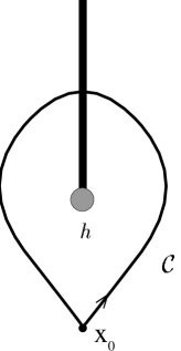
Figure 1.8: Single vortex solution. We have fixed the gauge freedom by sending all nontrivial parallel transport around the core in the Dirac string attached to the core. Thus outside the core, the Higgs field takes the same ground state value $\langle\Phi_{0}\rangle$ everywhere except for the region where the Dirac string is localized. Here it makes a noncontractible winding in the ground state manifold. This winding corresponds to a holonomy in the gauge field classified by the result of the untraced Wilson loop operator $W({\cal C},{\mbox{\bf x}}_{0})=h\in{H}_{0}$, which picks up the nonabelian magnetic flux located inside the core.

In this gauge fixed prescription, we are still able to perform global symmetry transformations $g\in{H}_{0}$ on these vortex solutions that leave the ground state $\langle\Phi_{0}\rangle$ invariant. These transformations affect the field configuration of the vortex in the following way

$$\Phi({\mbox{\bf x}}) \longmapsto g\;\Phi({\mbox{\bf x}})$$ (1.4.13)

$$A_{\kappa}({\mbox{\bf x}}) \longmapsto g\;A_{\kappa}({\mbox{\bf x}})\;g^{-1},$$ (1.4.14)

as an immediate consequence we then obtain

$$W({\cal C},{\mbox{\bf x}}_{0}) \longmapsto g\;W({\cal C},{\mbox{\bf x}}_{0})\;g^{-1},$$ (1.4.15)

which shows that the flux of the vortex becomes conjugated $h\mapsto ghg^{-1}$ under such a transformation. The conclusion is that these nonabelian vortex solutions are in fact organized in degenerate multiplets under the residual global symmetry transformations ${H}_{0}$, namely the different conjugacy classes of ${H}_{0}$ denoted as ${}^{A}C$, where $A$ labels a particular conjugacy class. For convenience, we will refer to the stability group of $\langle\Phi_{0}\rangle$ as ${H}$ from now on.

The different vortex solutions in a given conjugacy class ${}^{A}C$ of ${H}$, being related by internal global symmetry transformations that leave the action (1.4.1) invariant, clearly carry the same external quantum numbers, that is, the total energy of the configuration, the coresize etc. These solutions only differ by their internal magnetic flux quantum number. This internal degeneracy becomes relevant in adiabatic interchange processes of remote vortices in the plane. Consider, for instance, the configuration of two remote vortices as presented in figure 1.9. In the depicted adiabatic counterclockwise interchange of these vortices, the vortex initially carrying the magnetic flux $h_{2}$ moves through the Dirac string attached to the other vortex. As a result, its flux picks up a global symmetry transformation by the flux $h_{1}$ of the latter, i.e. $h_{2}\mapsto h_{1}h_{2}h^{-1}_{1}$, such that the total flux of the configuration is conserved. This classical nonabelian Aharonov-Bohm effect appearing for noncommuting fluxes, which has been called flux metamorphosis [16], leads to physical observable phenomena. Suppose, for example, that the magnetic flux $h_{2}$ was a member of a flux/anti-flux pair $(h_{2},h_{2}^{-1})$ created from the vacuum. When $h_{2}$ encircles $h_{1}$, it returns as the flux $h_{1}h_{2}h^{-1}_{1}$ and will not be able to annihilate the flux $h_{2}^{-1}$ anymore. Upon rejoining the pair we now obtain the stable flux $h_{1}h_{2}h^{-1}_{1}h_{2}$. Moreover, at the quantum level, flux metamorphosis leads to nontrivial Aharonov-Bohm scattering between nonabelian vortices as we will argue in more detail later on.

Residual global symmetry transformations naturally leave this observable Aharonov-Bohm effect for nonabelian vortices invariant. This simply follows from the fact that these transformations commute with this nonabelian Aharonov-Bohm effect. To be precise, a residual global symmetry transformation $g\in{H}$ on the two vortex configuration in figure 1.9, for example, affects the flux of both vortices through conjugation by the group element $g$, and it is easily verified that it makes no difference whether such a transformation is performed before the interchange is started or after the interchange is completed. The extension of these classical considerations to configurations of more then two vortices in the plane is straightforward. Braid processes, in which the fluxes of the vortices affect each other by conjugation, conserve the total flux of the configuration. The residual global symmetry transformations $g\in{H}$ of the low energy regime, which act by an overall conjugation of the fluxes of the vortices in the configuration by $g$, commute with these braid processes.

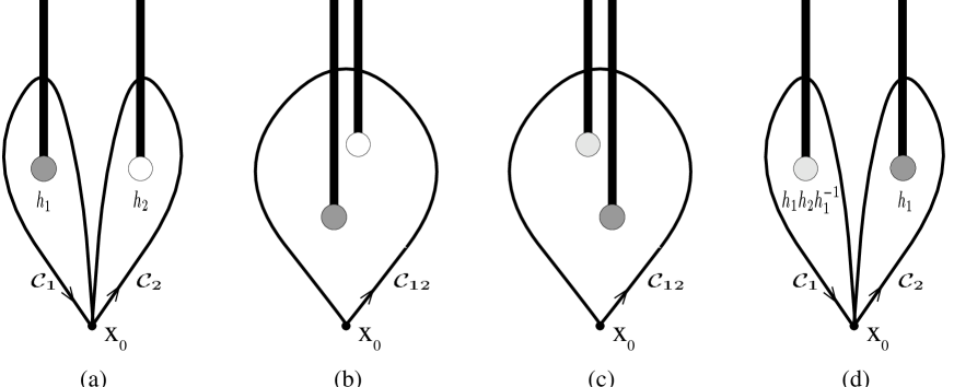
Figure 1.9: Flux metamorphosis. We start off with a classical configuration of two patched vortex solutions, as visualized in figure (a). The vortices are initially assumed to carry the fluxes $W({\cal C}_{1},{\mbox{\bf x}}_{0})=h_{1}$ and $W({\cal C}_{2},{\mbox{\bf x}}_{0})=h_{2}$. The total flux of this configuration is picked up by the Wilson line integral along the loop ${\cal C}_{12}$ encircling both vortices as depicted in figure (b): $W({\cal C}_{12},{\mbox{\bf x}}_{0})=W({\cal C}_{1}\circ{\cal C}_{2},{\mbox{\bf x}}_{0})=W({\cal C}_{1},{\mbox{\bf x}}_{0})\cdot W({\cal C}_{2},{\mbox{\bf x}}_{0})=h_{1}h_{2}$. Now suppose that the two vortices are interchanged in the counterclockwise fashion depicted in figures (b)-(d). In this process vortex 2 moves through the Dirac string attached to vortex 1 and as a result its flux will be affected $h_{2}\mapsto h_{2}^{\prime}$. Vortex 1, on the other hand, never meets any nontrivial parallel transport in the gauge fields and its flux remains the same. Since this local braid process should not be able to change the global properties of this system, i.e. the total flux, we have $h_{1}h_{2}=W({\cal C}_{12},{\mbox{\bf x}}_{0})=W({\cal C}_{1},{\mbox{\bf x}}_{0})\cdot W({\cal C}_{2},{\mbox{\bf x}}_{0})=h_{2}^{\prime}h_{1}$. Thus the flux of vortex 2 becomes conjugated $h_{2}^{\prime}=h_{1}h_{2}h^{-1}_{1}$ by the flux of vortex 1 in this braid process.

As in the abelian case discussed in the previous sections, we wish to treat these nonabelian vortices as point particles in the first quantized description. The degeneracy of these vortices under the residual global symmetry group ${H}$ then indicates that we have to assign a finite dimensional internal Hilbert space $V^{A}$ to these particles, which is spanned by the different fluxes in a given conjugacy class ${}^{A}C$ of ${H}$ and endowed with the standard inner product [18]

$$\langle h^{\prime}|h\rangle = \delta_{h^{\prime},h}\qquad\qquad\forall\,h,h^{\prime}\in\,^{A}C.$$ (1.4.16)

Under the residual global symmetry transformations the flux eigenstates in this internal Hilbert space $V^{A}$ are affected through conjugation

$$g\in{H}:\qquad|h\rangle \longmapsto |ghg^{-1}\rangle.$$ (1.4.17)

In general, the particle can be in a normalized linear combination of the different flux eigenstates in the internal Hilbert space $V^{A}$. The residual global symmetry transformations (1.4.17) act linearly on such states. Of course, the conjugated action of the residual symmetry group is in general reducible and, at first sight, it seems that we have to decompose this internal Hilbert space into the different irreducible components. This is not the case as we will see in more detail later on (see the discussion concerning relation (1.4.25)). The point is that we can independently perform physical flux measurements by means of quantum interference experiments with electric charges. These measurements project out a particular flux eigenstate. Clearly, these flux measurements do not commute with the residual global symmetry transformations and under their combined action the internal Hilbert spaces $V^{A}$ associated with the different conjugacy classes ${}^{A}C$ form irreducible representations.

The complete quantum state of these particles consists of an internal flux part and an external part. The quantum state describing a single particle in the flux eigenstate $|h_{1}\rangle\in V^{A_{1}}$ at a fixed position y in the plane, for instance, is the formal tensor product $|h_{1},{\mbox{\bf y}}\rangle=|h_{1}\rangle|{\mbox{\bf y}}\rangle$. To proceed, the initial configuration depicted in figure 1.9 is described by the multi-valued two particle quantum state $|h_{1},{\mbox{\bf y}}\rangle|h_{2},{\mbox{\bf z}}\rangle$, where again by convention the particle located most left in the plane appears most left in the tensor product. The result of an adiabatic counterclockwise interchange of the two particles can now be summarized by the action of the braid operator

$${\cal R}\;|h_{1},{\mbox{\bf y}}\rangle|h_{2},{\mbox{\bf z}}\rangle = |h_{1}h_{2}h^{-1}_{1},{\mbox{\bf y}}\rangle|h_{1},{\mbox{\bf z}}\rangle,$$ (1.4.18)

which acts linearly on linear combinations of these flux eigenstates. What we usually measure in quantum interference experiments, however, is the effect in the internal wave function of a monodromy of the two particles

$${\cal R}^{2}\;|h_{1},{\mbox{\bf y}}\rangle|h_{2},{\mbox{\bf z}}\rangle = |(h_{1}h_{2})h_{1}(h_{1}h_{2})^{-1},{\mbox{\bf y}}\rangle|h_{1}h_{2}h^{-1}_{1},{\mbox{\bf z}}\rangle.$$ (1.4.19)

This nonabelian Aharonov-Bohm effect can be probed either through a double slit experiment [8, 92] or through an Aharonov-Bohm scattering experiment as discussed in appendix 1.A. In the first case, we keep one particle fixed between the two slits, whereas the other particle comes in as a plane wave. The geometry of the Aharonov-Bohm scattering experiment, depicted in figure 1.13 is more or less similar. The interference pattern in both experiments is determined by the internal transition amplitude

$$\langle u_{2}|\langle u_{1}|\;{\cal R}^{2}\;|u_{1}\rangle|u_{2}\rangle,$$ (1.4.20)

where $|u_{1}\rangle$ and $|u_{2}\rangle$ respectively denote the properly normalized internal flux states of the two particles, which are generally linear combinations of the flux eigenstates in the corresponding internal Hilbert spaces $V^{A_{1}}$ and $V^{A_{2}}$. The topological interference amplitudes (1.4.20) summarize all the physical obervables for vortex configurations in the low energy regime to which we confine ourselves here. As we have argued before, the residual global symmetry transformations affect internal multi-vortex states through an overall conjugation

$$g\in{H}:\qquad|h_{1}\rangle|h_{2}\rangle \longmapsto |gh_{1}g^{-1}\rangle|gh_{2}g^{-1}\rangle,$$ (1.4.21)

which commutes with the braid operator and therefore leave the interference amplitudes (1.4.20) invariant.

1.4.3 Including matter

Let us now suppose that the total model is of the actual form

$$S = S_{\mbox{\scriptsize YMH}}+S_{\mbox{\scriptsize matter}},$$ (1.4.22)

where $S_{\mbox{\scriptsize YMH}}$ denotes the action for the nonabelian Higgs model given in (1.4.1) and the action $S_{\mbox{\scriptsize matter}}$ describes additional matter fields minimally coupled to the gauge fields. In principle, these matter fields correspond to multiplets which transform irreducibly under the spontaneously broken symmetry group ${G}$. Under the residual symmetry group ${H}$ in the Higgs phase, however, these representations will become reducible and branch to UIR’s $\Gamma$ of ${H}$. Henceforth, it is assumed that the matter content of the model is such that all UIR’s $\Gamma$ of ${H}$ are indeed realized. We will treat the different charges $\Gamma$, appearing in the Higgs phase in this way [7, 107], as point particles. In the first quantized description, these point charges then carry an internal Hilbert space, namely the representation space associated with $\Gamma$. Now suppose we have a configuration of a nonabelian vortex in a flux eigenstate $|h\rangle$ at some fixed position in the plane and a remote charge $\Gamma$ in a normalized internal charge state $|v\rangle$ fixed at another position. When the charge encircles the vortex in a counterclockwise fashion, it meets the Dirac string and picks up a global symmetry transformation by the flux of the vortex

$${\cal R}^{2}\;|h,{\mbox{\bf y}}\rangle|v,{\mbox{\bf z}}\rangle = |h,{\mbox{\bf y}}\rangle|\Gamma(h)\,v,{\mbox{\bf z}}\rangle,$$ (1.4.23)

where $\Gamma(h)$ is the matrix assigned to the group element $h$ in the representation $\Gamma$. The residual global symmetry transformations on this two particle configuration

$$g\in{H}:\qquad|h,{\mbox{\bf y}}\rangle|v,{\mbox{\bf z}}\rangle \longmapsto |ghg^{-1},{\mbox{\bf y}}\rangle|\Gamma(g)\,v,{\mbox{\bf z}}\rangle,$$ (1.4.24)

again commutes with this monodromy operation. Thus the interference amplitudes

$$\langle v|\langle h|\;{\cal R}^{2}\;|h\rangle|v\rangle = \langle h|h\rangle\langle v|\Gamma(h)\,v\rangle\;=\;\langle v|\Gamma(h)\,v\rangle,$$ (1.4.25)

measured in double slit or Aharonov-Bohm scattering experiments involving these particles are invariant under the residual global symmetry transformations. As alluded to before, these interference experiments can be used to measure the flux of a given vortex [8, 9, 92, 87]. To that end, we place the vortex between the two slits (or alternatively use it as the scatterer in an Aharonov-Bohm scattering experiment) and evaluate the interference pattern for an incident beam of charges $\Gamma$ in the same internal state $|v\rangle$. In this way, we determine the interference amplitude (1.4.25). Upon repeating this experiment a couple of times with different internal states for the incident charge $\Gamma$, we can determine all matrix elements of $\Gamma(h)$ and hence, iff $\Gamma$ corresponds to a faithful UIR of ${H}$, the group element $h$ itself. In a similar fashion, we may determine the charge $\Gamma$ of a given particle and, moreover, its internal quantum state $|v\rangle$. In this case, we put the unknown charge between the double slit (or use it as the scatterer in an Aharonov-Bohm scattering experiment), measure the interference pattern for an incident beam of vortices in the same flux eigenstate $|h\rangle$ and again repeat this experiment for all $h\in{H}$.

At this point, we have established the purely magnetic flux and the purely electric charge superselection sectors of the discrete gauge theory in the Higgs phase of the model (1.4.22). The different magnetic sectors are labeled by the conjugacy classes ${}^{A}C$ of ${H}$, whereas the different electric charge sectors correspond to the different UIR’s $\Gamma$ of the residual symmetry group ${H}$. The complete spectrum of this discrete gauge theory also contains dyonic combinations of these sectors. The relevant remark in this context is that we have not yet completely exhausted the action of the residual global symmetry transformations on the internal magnetic flux quantum numbers. As we have seen in (1.4.17), the residual global ${H}$ transformations affect the magnetic fluxes through conjugation. The transformations that slip through this conjugation may in principle be implemented on an additional internal charge degree of freedom assigned to these fluxes [18]. More specifically, the global symmetry transformations that leave a given flux $|h\rangle$ invariant are those that commute with this flux, i.e. the group elements in the centralizer ${}^{h}N\subset{H}$. The internal charges that we can assign to this flux correspond to the different UIR’s $\alpha$ of the group ${}^{h}N$. Hence, the inequivalent dyons that can be formed in the composition of a global ${H}$ charge $\Gamma$ with a magnetic flux $|h\rangle$ correspond to the different irreducible components of the subgroup ${}^{h}N$ of ${H}$ contained in the representation $\Gamma$. Two remarks are pertinent now. First of all, the centralizers of different fluxes in a given conjugacy class ${}^{A}C$ are isomorphic. Secondly, the full set of the residual global ${H}$ symmetry transformations relate the fluxes in a given conjugacy class carrying unitary equivalent centralizer charge representations. In other words, the different dyonic sectors are labeled by $(\,^{A}\!C,\alpha\,)$, where ${}^{A}\!C$ runs over the different conjugacy classes of ${H}$ and $\alpha$ over the different nontrivial UIR’s of the associated centralizer. The explicit transformation properties of these dyons under the full global group ${H}$ involve some conventions, which will be discussed in the algebraic approach to discrete ${H}$ gauge theories we take in the following section.

The physical observation behind this formal construction of the dyonic sectors is that we can in fact only measure the transformation properties of the charge of a given flux/charge composite under the centralizer of the flux of this composite [92]. A similar phenomenon occurs in the 3+1 dimensional setting for monopoles carrying a nonabelian magnetic charge where it is known as the global color problem [97, 23, 98]. To illustrate this phenomenon, we suppose that we have a composite of a pure flux $|h\rangle$ and a pure global ${H}$ charge $\Gamma$ in some internal state $|v\rangle$. Thus the complete internal state of the composite becomes $|h,v\rangle$. As we have argued before, the charge of a given object can be determined through double slit or Aharonov-Bohm scattering experiments involving beams of vortices in the same internal flux state $|h^{\prime}\rangle$ and repeating these experiments for all $h^{\prime}\in{H}$. The interference amplitudes measured in this particular case are of the form

$$\langle h,v|\langle h^{\prime}|\;{\cal R}^{2}\;|h^{\prime}\rangle|h,v\rangle = \langle h,v|h^{\prime}hh^{\prime-1},\Gamma(h^{\prime})\,v\rangle\langle h^{\prime}|(h^{\prime}h)h^{\prime}(h^{\prime}h)^{-1}\rangle$$

$$= \langle v|\Gamma(h^{\prime})\,v\rangle\>\delta_{h,h^{\prime}hh^{\prime-1}}\;,$$

where we used (1.4.19) and (1.4.23). As a result of the flux metamorphosis (1.4.19), the interference term is only nonzero for experiments involving fluxes $h^{\prime}$ that commute with the flux of the composite, i.e. $h^{\prime}\in$$\,{}^{h}N$. Thus we are only able to detect the response of the charge $\Gamma$ of the composite to global symmetry transformations in ${}^{h}N$. This topological obstruction is usually summarized with the statement [24, 116, 5, 107] that in the background of a single vortex $h$, the only ‘realizable’ global symmetry transformations are those taking values in the centralizer ${}^{h}N$.

Let us close this section with a summary of the main conclusions. First of all, the complete spectrum of the nonabelian discrete ${H}$ gauge theory appearing in the Higgs phase of the model (1.4.22) can be presented as

$$(\,^{A}\!C,\alpha\,),$$ (1.4.27)

where ${}^{A}\!C$ runs over the conjugacy classes of ${H}$ and $\alpha$ denotes the different UIR’s of the centralizer associated to a specific conjugacy class ${}^{A}\!C$. The purely magnetic sectors correspond to trivial centralizer representations and are labeled by the different nontrivial conjugacy classes. The pure charge sectors, on the other hand, correspond to the trivial conjugacy class (with centralizer the full group ${H}$) and are labeled by the different nontrivial UIR’s of the residual symmetry group ${H}$. The other sectors describe the dyons in this theory. Note that the sectors (1.4.27) boil down to the sectors of the spectrum (1.3.33) in case ${H}\simeq{\mbox{\bf Z}}_{N}$.

The remaining long range interactions between the particles (1.4.27) are topological Aharonov-Bohm interactions. In a counterclockwise braid process involving two given particles, the internal quantum state of the particle that moves through the Dirac string attached to the flux of the other particle picks up a global symmetry transformation by this flux. This (in general nonabelian) Aharonov-Bohm effect conserves the total flux of the system and moreover commutes with the residual global ${H}$ transformations, which act simultaneously on the internal quantum states of all the particles in the system. The last property ensures that the physical observables for a given system, which are all related to this Aharonov-Bohm effect, are invariant under global ${H}$ transformations.

An exhaustive discussion of the braid and fusion properties of the particles in the spectrum (1.4.27) involves the algebraic structure underlying a discrete ${H}$ gauge theory, which will be revealed in the next section. For notational simplicity, we will omit explicit mentioning of the external degrees of freedom of the particles in the following. In our considerations, we usually work with position eigenstates for the particles unless we are discussing double slit- or Aharonov-Bohm scattering experiments in which the incoming projectiles are in momentum eigenstates.

1.5 Quantum doubles

It is by now well-established that there are deep connections between two dimensional rational conformal field theory, three dimensional topological field theory and quantum groups or Hopf algebras (see for instance [14, 15, 136] and references therein). Discrete $H$ gauge theories, being examples of three dimensional topological field theories, naturally fit in this general scheme. The algebraic structure underlying a discrete $H$ gauge theory is the Hopf algebra $D(H)$ [18, 19, 20]. This is the quasitriangular Hopf algebra obtained from Drinfeld’s quantum double construction [51, 52] as applied to the abelian algebra ${\cal F}(H)$ of functions on the finite group ${H}$. (For a thorough treatment of Hopf algebras in general and related issues, the interested reader is referred to the excellent book by Shnider and Sternberg [118]). Considered as a vector space, we then have $D(H)={\cal F}(H)\otimes{\bf C}[H]$, where ${\bf C}[H]$ denotes the group algebra over the complex numbers ${\bf C}$. Roughly speaking, the elements of $D(H)$ signal the flux of the particles (1.4.27) and implement the residual global symmetry transformations. Under this action the particles form irreducible representations. Moreover, the algebra $D({H})$ provides an unified description of the braiding and fusion properties of the particles. Henceforth, we will simply refer to the algebra $D({H})$ as the quantum double. This name, inspired by its mathematical construction, also summarizes nicely the physical content of a Higgs phase with a residual finite gauge group $H$. The topological interactions between the particles are of a quantum mechanical nature, whereas the spectrum (1.4.27) exhibits an electric/magnetic self-dual (or double) structure.

In fact, the quantum double $D({H})$ was first proposed by Dijkgraaf, Pasquier and Roche [46]. They identified it as the Hopf algebra associated with certain holomorphic orbifolds of rational conformal field theories [48] and the related three dimensional topological field theories with finite gauge group $H$ as introduced by Dijkgraaf and Witten [47]. The new insight that emerged in [18, 19, 20] was that such a topological field theory finds a natural realization as the residual discrete $H$ gauge theory describing the long range physics of gauge theories in which a continuous gauge group $G$ is spontaneously broken down to a finite group $H$.

1.5.1 $D({H})$

As we have seen in the previous sections, we are basically left with two physical operations on the particles (1.4.27) in the spectrum of a discrete ${H}$ gauge theory. We can independently measure their flux and their charge through quantum interference experiments. The fluxes are the group elements $h\in{H}$, while the dyon charges are the representations of the centralizer of this particular flux. Flux measurements correspond to operators ${\mbox{P}}_{h}$ projecting out a particular flux $h$, while the charge of a particle can be detected through its transformation properties under the residual global symmetry transformations $g\in{H}$ that commute with the flux of the particle. The operators ${\mbox{P}}_{h}$ projecting out the flux $h\in{H}$ of a given quantum state naturally realize the projector algebra

$${\mbox{P}}_{h}{\mbox{P}}_{h^{\prime}} = \delta_{h,h^{\prime}}\;{\mbox{P}}_{h},$$ (1.5.1)

with $\delta_{h,h^{\prime}}$ the kronecker delta function for the group elements $h,h^{\prime}\in{H}$. As we have seen in (1.4.17), global symmetry transformations $g\in{H}$ affect the fluxes through conjugation, which implies that the flux projection operators and global symmetry transformations do not commute

$$g\,{\mbox{P}}_{h} = {\mbox{P}}_{ghg^{-1}}\,g.$$ (1.5.2)

The combination of global symmetry transformations followed by flux measurements

$$\{{\mbox{P}}_{h}\,g\}_{h,g\in{H}},$$ (1.5.3)

generate the quantum double $D({H})={\cal F}(H)\otimes{\bf C}[H]$ and the multiplication (1.5.1) and (1.5.2) of these elements can be recapitulated as 

$${\mbox{P}}_{h}\,g\cdot{\mbox{P}}_{h^{\prime}}\,g^{\prime} = \delta_{h,gh^{\prime}g^{-1}}\;{\mbox{P}}_{h}\,gg^{\prime}.$$ (1.5.4)

The different particles (1.4.27) in the spectrum of the associated discrete ${H}$ gauge theory constitute the complete set of inequivalent irreducible representations of the quantum double $D({H})$. To make explicit the irreducible action of the quantum double on these particles, we have to develop some further notation. To start with, we will label the group elements in the different conjugacy classes of ${H}$ as

$${}^{A}\!C = \{^{A}\!h_{1},\;^{A}\!h_{2},\ldots,\,^{A}\!h_{k}\}.$$ (1.5.5)

Let ${}^{A}\!N\subset{H}$ be the centralizer of the group element ${}^{A}\!h_{1}$ and $\{^{A}\!x_{1},\,^{A}\!x_{2},\ldots,\,^{A}\!x_{k}\}$ a set of representatives for the equivalence classes of ${H}/^{A}\!N$, such that ${}^{A}\!h_{i}=\,^{A}\!x_{i}\,^{A}\!h_{1}\,^{A}\!x_{i}^{-1}$. For convenience, we will always take ${}^{A}\!x_{1}=e$, with $e$ the unit element in ${H}$. To proceed, the basis vectors of the unitary irreducible representation ${\alpha}$ of the centralizer ${}^{A}\!N$ will be denoted by ${}^{\alpha}\!v_{j}$. With these conventions the internal Hilbert space $V^{A}_{\alpha}$ is spanned by the quantum states

$$\{|\,^{A}\!h_{i},\,^{\alpha}\!v_{j}\rangle\}_{i=1,\ldots,k}^{j=1,\ldots,\mbox{\scriptsize dim}{\,\alpha}}.$$ (1.5.6)

The combined action of a global symmetry transformation $g\in{H}$ followed by a flux projection operator ${\mbox{P}}_{h}$ on these internal flux/charge eigenstates spanning the Hilbert space $V^{A}_{\alpha}$ can then be presented as [46]

$$\Pi^{A}_{\alpha}(\,{\mbox{P}}_{h}\,{g}\,)\;|\,^{A}\!h_{i},\,^{\alpha}\!v_{j}\rangle = \delta_{h,g\,^{A}\!h_{i}\,g^{-1}}\;\;|\,g\,^{A}\!h_{i}\,g^{-1},\,{\alpha}(\tilde{g})_{mj}\,^{\alpha}v_{m}\rangle,$$ (1.5.7)

with

$$\tilde{g} := \,{}^{A}\!x_{k}^{-1}\,g\,\,^{A}\!x_{i},$$ (1.5.8)

and $\,{}^{A}\!x_{k}$ defined through $\,{}^{A}\!h_{k}:=g\,^{A}\!h_{i}\,g^{-1}$. It is easily verified that this element $\tilde{g}$ constructed from $g$ and the flux ${}^{A}\!h_{i}$ indeed commutes with ${}^{A}\!h_{1}$ and therefore can be implemented on the centralizer charge. Two remarks are pertinent now. First of all, there is of course arbitrariness involved in the ordering of the elements in the conjugacy classes and the choice of the representatives $\,{}^{A}\!x_{k}$ for the equivalence classes of the coset ${H}/^{A}\!N$. However, different choices lead to unitarily equivalent representations of the quantum double. Secondly, note that (1.5.7) is exactly the action anticipated in section 1.4. The flux ${}^{A}\!h_{i}$ of the associated particle is conjugated by the global symmetry transformation $g\in{H}$, while the part of $g$ that slips through this conjugation is implemented on the centralizer charge of the particle. The operator ${\mbox{P}}_{h}$ subsequently projects out the flux $h$.

We will now argue that the flux/charge eigenstates (1.5.6) spanning the internal Hilbert space $V^{A}_{\alpha}$ carry the same spin, i.e. a counterclockwise rotation over an angle of $2\pi$ gives rise to the same spin factor for all quantum states in $V^{A}_{\alpha}$. As in our discussion of abelian dyons in section 1.3.3, we assume a small seperation between the centralizer charge and the flux of the dyons. In the aforementioned rotation, the centralizer charge of the dyon then moves through the Dirac string attached to the flux of the dyon and as a result picks up a transformation by this flux. The element in the quantum double that implements this effect on the internal quantum states (1.5.6) is the central element

$$\sum_{h}\;{\mbox{P}}_{h}\,h.$$ (1.5.9)

It signals the flux of the internal quantum state and implements this flux on the centralizer charge

$$\Pi^{A}_{\alpha}(\,\sum_{h}\;{\mbox{P}}_{h}\,h\,)\;|\,^{A}\!h_{i},\,^{\alpha}\!v_{j}\rangle = |\,^{A}\!h_{i},\,{\alpha}(^{A}\!h_{1})_{mj}\,^{\alpha}v_{m}\rangle,$$ (1.5.10)

which boils down to the same matrix ${\alpha}(^{A}\!h_{1})$ for all fluxes ${}^{A}\!h_{i}$ in ${}^{A}\!C$. Here we used (1.5.7) and (1.5.8). Since ${}^{A}\!h_{1}$ by definition commutes with all the elements in the centralizer ${}^{A}\!N$, it follows from Schur’s lemma that it is proportional to the unit matrix in the irreducible representation $\alpha$

$${\alpha}(^{A}\!h_{1}) = e^{2\pi\imath s_{(A,\alpha)}}\,{\mbox{\bf 1}}_{\alpha}.$$ (1.5.11)

This proves our claim. The conclusion is that there is an overall spin value $s_{(A,\alpha)}$ assigned to the sector $(\,^{A}\!C,\alpha\,)$. Note that the only sectors carrying a nontrivial spin are the dyonic sectors corresponding to nontrivial conjugacy classes paired with nontrivial centralizer charges.

The internal Hilbert space describing a system of two particles $(\,^{A}C,\alpha\,)$ and $(\,^{B}C,\beta\,)$ is the tensor product $V_{\alpha}^{A}\otimes V_{\beta}^{B}$. The extension of the action of the quantum double $D({H})$ on the single particle states (1.5.7) to the two particle states in $V_{\alpha}^{A}\otimes V_{\beta}^{B}$ is given by the comultiplication

$$\Delta(\,{\mbox{P}}_{h}\,g\,) = \sum_{h^{\prime}\cdot h^{\prime\prime}=h}{\mbox{P}}_{h^{\prime}}\,g\otimes{\mbox{P}}_{h^{\prime\prime}}\,{g},$$ (1.5.12)

which is an algebra morphism from $D({H})$ to $D({H})\otimes D({H})$. To be concrete, the tensor product representation of $D({H})$ carried by the two particle internal Hilbert space $V_{\alpha}^{A}\otimes V_{\beta}^{B}$ is defined as $\Pi^{A}_{\alpha}\otimes\Pi^{B}_{\beta}(\Delta(\,{\mbox{P}}_{h}\,g\,))$. The action (1.5.12) of the quantum double on the internal two particle quantum states in $V_{\alpha}^{A}\otimes V_{\beta}^{B}$ can be summarized as follows. In accordance with our observations in the previous section, the residual global symmetry transformations $g\in{H}$ affect the internal quantum states of the two particles separately. The projection operator ${\mbox{P}}_{h}$ subsequently projects out the total flux of the two particle quantum state. Hence the action (1.5.12) of the quantum double determines the global properties of a given two particle quantum state, which are conserved under the local process of fusing the two particles. It should be mentioned now that the tensor product representation $(\Pi^{A}_{\alpha}\otimes\Pi^{B}_{\beta},V_{\alpha}^{A}\otimes V_{\beta}^{B})$ of $D({H})$ is in general reducible, and can be decomposed into a direct sum of irreducible representations $(\Pi^{C}_{\gamma},V^{C}_{\gamma})$. The different single particle states that can be obtained by the aforementioned fusion process are the states in the different internal Hilbert spaces $V^{C}_{\gamma}$ that occur in this decomposition. We will return to an elaborate discussion of the fusion rules in section 1.5.3.

An important property of the comultiplication (1.5.12) is that it is coassociative

$$({\mbox{id}}\otimes\Delta)\,\Delta(\,{\mbox{P}}_{h}\,g\,)=(\Delta\otimes{\mbox{id}})\,\Delta(\,{\mbox{P}}_{h}\,g\,)=\sum_{h^{\prime}\cdot h^{\prime\prime}\cdot h^{\prime\prime\prime}=h}{\mbox{P}}_{h^{\prime}}\,g\otimes{\mbox{P}}_{h^{\prime\prime}}\,{g}\otimes{\mbox{P}}_{h^{\prime\prime\prime}}\,{g}.$$ (1.5.13)

This means that the representation of the quantum double on the internal Hilbert space $V_{\alpha}^{A}\otimes V_{\beta}^{B}\otimes V_{\gamma}^{C}$ (describing a system of three particles) either through $({\mbox{id}}\otimes\Delta)\,\Delta$ or through $(\Delta\otimes{\mbox{id}})\,\Delta$ is completely equivalent. Extending the action of the quantum double to systems containing an arbitrary number of particles is now straightforward. The global symmetry transformations $g\in{H}$ are implemented on all the particles separately, while the operator ${\mbox{P}}_{h}$ projects out the total flux of the system.

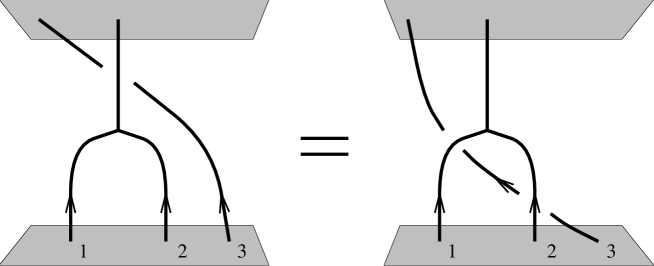
Figure 1.10: Compatibility of fusion and braiding as expressed by the quasitriangularity conditions. It makes no difference whether a third particle braids with two particles separately or with the composite that arises after fusing these two particles. We have depicted the trajectories of the particles as lines instead of ribbons. This is what we will usually do when there is no writhing involved in the argument.

The braid operation is formally implemented by the universal $R$-matrix, which is an element of $D({H})\otimes D({H})$

$$R = \sum_{h,g}\,{\mbox{P}}_{g}\otimes{\mbox{P}}_{h}\,{g}.$$ (1.5.14)

The $R$ matrix acts on a two particle state as a global symmetry transformation on the second particle by the flux of the first particle. The physical braid operator ${\cal R}$ that effectuates a counterclockwise interchange of the two particles is defined as the action of this $R$ matrix followed by a permutation $\sigma$ of the two particles

$${\cal R}_{\alpha\beta}^{AB} := \sigma\circ(\Pi_{\alpha}^{A}\otimes\Pi_{\beta}^{B})(\,R\,),$$ (1.5.15)

To be explicit, on the two particle state $|\,^{A}\!h_{i},\,^{\alpha}\!v_{j}\rangle|\,^{B}\!h_{m},\,^{\beta}\!v_{n}\rangle\in V^{A}_{\alpha}\otimes V^{B}_{\beta}$ we have

$${\cal R}\;|\,^{A}\!h_{i},\,^{\alpha}\!v_{j}\rangle|\,^{B}\!h_{m},\,^{\beta}\!v_{n}\rangle = |\,^{A}\!h_{i}\,^{B}\!h_{m}\,^{A}\!h_{i}^{-1},\,\beta(\,^{A}\!\tilde{h}_{i}\,)_{ln}\,^{\beta}\!v_{l}\rangle|\,^{A}\!h_{i},\,^{\alpha}\!v_{j}\rangle,$$ (1.5.16)

where the element ${}^{A}\!\tilde{h}_{i}$ is defined as in (1.5.8). Note that the expression (1.5.16), which summarizes the braid operation on all conceivable two particle states in this theory, contains the braid effects established in the previous section, namely flux metamorphosis for two pure magnetic fluxes (1.4.18) and the Aharonov-Bohm effect for a pure magnetic flux with a pure charge (1.4.23).

It is easily verified that the braid operator (1.5.16) and the comultiplication (1.5.12) satisfy the quasitriangularity conditions

$${\cal R}\>\Delta(\,{\mbox{P}}_{h}\,g\,) = \Delta(\,{\mbox{P}}_{h}\,g\,)\>{\cal R}$$ (1.5.17)

$$({\mbox{id}}\otimes\Delta)({\cal R}) = {\cal R}_{2}\;{\cal R}_{1}$$ (1.5.18)

$$(\Delta\otimes{\mbox{id}})({\cal R}) = {\cal R}_{1}\;{\cal R}_{2}.$$ (1.5.19)

where the braid operators ${\cal R}_{1}$ and ${\cal R}_{2}$ respectively act as ${\cal R}\otimes{\mbox{\bf 1}}$ and ${\mbox{\bf 1}}\otimes{\cal R}$ on three particle states in $V_{\alpha}^{A}\otimes V_{\beta}^{B}\otimes V_{\gamma}^{C}$. The relation (1.5.17) expresses the fact that the braid operator commutes with the global symmetry transformations $g\in{H}$ and conserves the total magnetic flux of the configuration as measured by ${\mbox{P}}_{h}$. In addition, the quasitriangularity conditions (1.5.18) and (1.5.19), which can be presented graphically as in figure 1.10, imply consistency between braiding and fusing. From this set of quasitriangularity conditions, it follows that the braid operator satisfies the Yang-Baxter equation

$${\cal R}_{1}\;{\cal R}_{2}\;{\cal R}_{1} = {\cal R}_{2}\;{\cal R}_{1}\;{\cal R}_{2}.$$ (1.5.20)

Thus the braid operators (1.5.16) define representations of the braid groups discussed in section 1.2. These unitary representations are in general reducible. So the internal Hilbert space describing a multi-particle system in general splits up into a direct sum of irreducible subspaces under the action of the braid group. The braid properties of the system depend on the particular irreducible subspace. If the dimension of the irreducible representation is one, we are dealing with abelian braid statistics or ordinary anyons. If the dimension is larger then one, we are dealing with nonabelian braid statistics, i.e. the nonabelian generalization of anyons. Note that these higher dimensional irreducible representations only occur for systems consisting of more than two particles, because the braid group for two particles is abelian.

To conclude, the internal Hilbert space describing a multi-particle system carries a representation of the internal symmetry algebra $D({H})$ and a braid group representation. Both representations are in general reducible. The quasitriangularity condition (1.5.17) implies (see for instance [14, 15]) that the action of the associated braid operators commutes with the action of the elements of $D({H})$. Thus the multi-particle internal Hilbert space can in fact be decomposed into a direct sum of irreducible subspaces under the direct product action of $D({H})$ and the braid group. We discuss this in further detail in the next two sections. We first introduce the notion of truncated braid groups.

1.5.2 Truncated braid groups

We turn to a closer examination of the braid group representations that occur in discrete ${H}$ gauge theories. An important observation in this respect is that the braid operator (1.5.16) is of finite order

$${\cal R}^{m} = {\mbox{\bf 1}}\otimes{\mbox{\bf 1}},$$ (1.5.21)

with 1 the identity operator and $m$ some integer depending on the specific particles on which the braid operator acts. In other words, we can assign a finite number $m$ to any two particle internal Hilbert space $V_{\alpha}^{A}\otimes V_{\beta}^{B}$, such that the effect of $m$ braidings is trivial for all states in this internal Hilbert space. This result, which can be traced back directly to the finite order of ${H}$, implies that the multi-particle configurations appearing in a discrete ${H}$ gauge theory actually realize representations of factor groups of the braid groups discussed in section 1.2. Consider, for instance, a system consisting of $n$ indistinguishable particles. Thus all particles carry the same internal Hilbert space $V^{A}_{\alpha}$ and the $n$ particle internal Hilbert space describing this system is the tensor product space $(V^{A}_{\alpha})^{\otimes n}$. The abstract generator $\tau_{i}$, which establishes a counterclockwise interchange of the two adjacent particles $i$ and $i+1$, acts on this internal Hilbert space by means of the operator

$$\tau_{i} \longmapsto {\cal R}_{i}\,,$$ (1.5.22)

with

$${\cal R}_{i} := {\mbox{\bf 1}}^{\otimes(i-1)}\otimes{\cal R}\otimes{\mbox{\bf 1}}^{\otimes(n-i-1)}.$$ (1.5.23)

Hence, the generator $\tau_{i}$ acts as (1.5.16) on the $i^{\rm th}$ and $(i+1)^{\rm th}$ entry in the tensor product space $(V^{A}_{\alpha})^{\otimes n}$. As follows from (1.5.20) and (1.5.21), the homomorphism (1.5.22) furnishes a representation of the braid group

$$\begin{array}[]{rcll}\tau_{i}\tau_{i+1}\tau_{i}&=&\tau_{i+1}\tau_{i}\tau_{i+1}&\qquad i=1,\ldots,n-2\\ \tau_{i}\tau_{j}&=&\tau_{j}\tau_{i}&\qquad|i-j|\geq 2,\end{array}$$ (1.5.26)

with the extra relation

$$\tau_{i}^{m} = e\;\;\;\;\;\;\;\;\;\;i=1,\ldots,n-1.$$ (1.5.27)

where $e$ denotes the unit element or trivial braid. For obvious reasons, we will call the factor groups with defining relations (1.5.26) and the additional relation (1.5.27) truncated braid groups $B(n,m)$, where $n$ stands for the number of particles and $m$ for the order of the generators $\tau_{i}$.

This picture naturally extends to a system containing $n$ distinguishable particles, i.e. the particles carry different internal Hilbert spaces or ‘colors’ now. The group that governs the monodromy properties of such a system is the truncated version $P(n,m)$ of the colored braid group $P_{n}({\mbox{\bf R}}^{2})$ defined in (1.2.7). To be specific, the truncated colored braid group $P(n,m)$ is the subgroup of $B(n,m)$ generated by

$$\gamma_{ij} = \tau_{i}\cdots\tau_{j-2}\;\tau_{j-1}^{2}\;\tau_{j-2}^{-1}\cdots\tau_{i}^{-1}\qquad\qquad 1\leq i<j\leq n,$$ (1.5.28)

with the extra relation (1.5.27) incorporated. Thus the generators of the pure braid group satisfy

$$\gamma_{ij}^{m/2} = e,$$ (1.5.29)

from which it is clear that the colored braid group $P(n,m)$ can only be defined for even $m$. The representation of the colored braid group $P(n,m)$ realized by a system of $n$ different particles then becomes

$$\gamma_{ij} \longmapsto {\cal R}_{i}\cdots{\cal R}_{j-1}\;{\cal R}_{j}^{2}\;{\cal R}_{j-1}^{-1}\cdots{\cal R}_{i}^{-1},$$ (1.5.30)

where the operators ${\cal R}_{i}$ defined by expression (1.5.23) now act on the tensor product space $V^{A_{1}}_{\alpha_{1}}\otimes\cdots\otimes V^{A_{n}}_{\alpha_{n}}$ of $n$ different internal Hilbert spaces $V^{A_{l}}_{\alpha_{l}}$.

Finally, a mixture of the above systems is of course also possible, that is, a system containing a subsystem consisting of $n_{1}$ particles with ‘color’ $V^{A_{1}}_{\alpha_{1}}$, a subsystem of $n_{2}$ particles carrying the different ‘color’ $V^{A_{2}}_{\alpha_{2}}$ and so on. Such a system realizes a representation of a truncated partially colored braid group (see for instance [32, 33] for the definition of ordinary partially colored braid groups). Let $n$ again be the total number of particles in the system. The truncated partially colored braid group associated with this system then becomes the subgroup of $B(n,m)$, generated by the braid operations on particles with the same ‘color’ and the monodromy operations on particles carrying different ‘color’.

The appearance of truncated rather than ordinary braid groups facilitates the decomposition of a given multi-particle internal Hilbert space into irreducible subspaces under the braid/monodromy operations. The point is that the representation theory of ordinary braid groups is rather complicated due to their infinite order. The extra relation (1.5.27) for truncated braid groups $B(n,m)$, however, causes these to become finite for various values of the labels $n$ and $m$, which leads to identifications with well-known groups of finite order [50]. It is instructive to consider some of these cases explicitly. The truncated braid group $B(2,m)$ for two indistinguishable particles, for instance, has only one generator $\tau$, which satisfies $\tau^{m}=e$. Thus we obtain the isomorphism

$$B(2,m) \simeq {\mbox{\bf Z}}_{m}.$$ (1.5.31)

For $m=2$, the relations (1.5.26) and (1.5.27) are the defining relations of the permutation group $S_{n}$ on $n$ strands

$$B(n,2) \simeq S_{n}.$$ (1.5.32)

A less trivial example is the nonabelian truncated braid group $B(3,3)$ for 3 indistinguishable particles. By explicit construction from the defining relations (1.5.26) and (1.5.27), we arrive at the identification

$$B(3,3) \simeq \bar{T},$$ (1.5.33)

with $\bar{T}$ the lift of the tetrahedral group into $SU(2)$. The structure of the truncated braid group $B(3,4)$ and its subgroup $P(3,4)$, which for example occur in a $\bar{D}_{2}$ gauge theory (see section 1.6.3), can be found in appendix 1.B.

To our knowledge, truncated braid groups have not been studied in the literature so far and a complete classification is not available. Although discrete ${H}$ gauge theories just realize finite dimensional representations, it remains an interesting group theoretical question whether the truncated braid groups are of finite order for all values of the labels $n$ and $m$.

1.5.3 Fusion, spin, braid statistics and all that $\dots$

Let $(\Pi^{A}_{\alpha},V_{\alpha}^{A})$ and $(\Pi^{B}_{\beta},V_{\beta}^{B})$ be two irreducible representations of the quantum double $D({H})$ as defined in (1.5.7). The tensor product representation $(\Pi^{A}_{\alpha}\otimes\Pi^{B}_{\beta},V_{\alpha}^{A}\otimes V_{\beta}^{B})$, constructed by means of the comultiplication (1.5.12), need not be irreducible. In general, it gives rise to a decomposition

$$\Pi^{A}_{\alpha}\otimes\Pi^{B}_{\beta} = \bigoplus_{C,\gamma}N^{AB\gamma}_{\alpha\beta C}\;\Pi^{C}_{\gamma},$$ (1.5.34)

where $N^{AB\gamma}_{\alpha\beta C}$ stands for the multiplicity of the irreducible representation $(\Pi^{C}_{\gamma},V^{C}_{\gamma})$. From the orthogonality relation for the characters of the irreducible representations of $D({H})$, we infer [46]

$$N^{AB\gamma}_{\alpha\beta C} = \frac{1}{|{H}|}\sum_{h,g}\;\mbox{tr}\left(\Pi^{A}_{\alpha}\otimes\Pi^{B}_{\beta}(\Delta(\,{\mbox{P}}_{h}\,g\,))\right)\;\mbox{tr}\left(\Pi^{C}_{\gamma}(\,{\mbox{P}}_{h}\,g\,)\right)^{*},$$ (1.5.35)

where $|{H}|$ denotes the order of the group ${H}$ and $*$ indicates complex conjugation. The fusion rule (1.5.34) now determines which particles $(\,^{C}C,\gamma)$ can be formed in the composition of the two particles $(\,^{A}C,\alpha\,)$ and $(\,^{B}C,\beta\,)$, or if read backwards, gives the decay channels of the particle $(\,^{C}C,\gamma\,)$.

The fusion algebra, spanned by the elements $\Pi^{A}_{\alpha}$ with multiplication rule (1.5.34), is commutative and associative and can therefore be diagonalized. The matrix implementing this diagonalization is the modular $S$ matrix [125]

$$S^{AB}_{\alpha\beta} := \frac{1}{|{H}|}\,\mbox{tr}\;{\cal R}^{-2\;AB}_{\;\;\;\;\;\alpha\beta}$$

$$= \frac{1}{|{H}|}\,\sum_{\stackrel{{\,{}^{A}\!h_{i}\in\,^{A}\!C\,,^{B}\!h_{j}\in\,^{B}\!C}}{{[\,^{A}\!h_{i},\,^{B}\!h_{j}]=e}}}\mbox{tr}\left(\alpha(\,^{A}\!x_{i}^{-1}\,{}^{B}\!h_{j}\,^{A}\!x_{i})\right)^{*}\;\mbox{tr}\left(\beta(\,^{B}\!x_{j}^{-1}\,{}^{A}\!h_{i}\,^{B}\!x_{j})\right)^{*},$$

which contains all information concerning the fusion algebra (1.5.34). In particular, the multiplicities (1.5.35) can be expressed in terms of the modular $S$ matrix by means of Verlinde’s formula [125]

$$N^{AB\gamma}_{\alpha\beta C} = \sum_{D,\delta}\frac{S^{AD}_{\alpha\delta}S^{BD}_{\beta\delta}(S^{*})^{CD}_{\gamma\delta}}{S^{eD}_{0\delta}}.$$ (1.5.37)

Whereas the modular $S$ matrix is determined through the monodromy operator following from (1.5.16), the modular matrix $T$ contains the spin factors (1.5.11) assigned to the particles

$$T^{AB}_{\alpha\beta} := \delta_{\alpha,\beta}\,\delta^{A,B}\;\exp(2\pi\imath s_{(A,\alpha)})\;=\;\delta_{\alpha,\beta}\,\delta^{A,B}\frac{1}{d_{\alpha}}\,\mbox{tr}\left(\alpha(^{A}\!h_{1})\right),$$ (1.5.38)

with $d_{\alpha}$ the dimension of the centralizer charge representation $\alpha$ of the particle $(\,^{A}C,\alpha\,)$. The matrices (1.5.3) and (1.5.38) now realize an unitary representation of the modular group $SL(2,{\mbox{\bf Z}})$ with the following relations [48]

$$\halign to=0.0pt{\hskip\@centering$\displaystyle{#}$\@eqnsel&\global\@eqcnt\@ne\hskip\tw@\arraycolsep\hfil${#}$\hfil&\global\@eqcnt\tw@\hskip\tw@\arraycolsep$\displaystyle{#}$\hfil&\global\@eqcnt\thr@@\hskip\tw@\arraycolsep\hfil\hbox{#}&\global\@eqcnt 4 \hbox\bgroup\hss#\egroup\cr 0.0pt plus 1000.0pt$\displaystyle{{\cal C} &10.0pt\hfil${=&10.0pt$\displaystyle{(ST)^{3} \; = \; S^{2}, &10.0pt\hfil\hbox{ \\ S^* &{\hss=}&{\cal C}S\;=\;S^{-1},&$\qquad S^t \;=\; S, $\\T^{*}&=&T^{-1},&$\qquad T^t \;=\; T.$(1.5.39)\cr}}}}}$$

The relations (1.5.3) and (1.5.3) express the fact that the matrices (1.5.3) and (1.5.38) are symmetric and unitary. To proceed, the matrix ${\cal C}$ defined in (1.5.3) represents the charge conjugation operator, which assigns an unique anti-partner ${\cal C}\,(\,^{A}C,\alpha\,)=(\,^{\bar{A}}C,\bar{\alpha}\,)$ to every particle $(\,^{A}C,\alpha\,)$ in the spectrum, such that the vacuum channel occurs in the fusion rule (1.5.34) for the particle/anti-particle pairs. Also note that the complete set of relations imply that the charge conjugation matrix ${\cal C}$ commutes with the modular matrix $T$, from which we conclude that a given particle carries the same spin as its anti-partner.

Having determined the fusion rules and the associated modular algebra, we turn to the issue of braid statistics and the fate of the spin statistics connection in this nonabelian context. Let us emphasize from the outset that much of what follows has been established elsewhere in a more general setting. See [14, 15] and the references therein for the conformal field theory point of view and [60, 61, 136] for the related 2+1 dimensional space time perspective.

We first discuss a system consisting of two distinguishable particles $(\,^{A}C,\alpha\,)$ and $(\,^{B}C,\beta\,)$. The associated two particle internal Hilbert space $V_{\alpha}^{A}\otimes V_{\beta}^{B}$ carries a representation of the abelian truncated colored braid group $P(2,m)$ with $m/2\in{\mbox{\bf Z}}$ the order of the monodromy matrix ${\cal R}^{2}$ for this particular two-particle system. This representation decomposes into a direct sum of one dimensional irreducible subspaces, each being labeled by the associated eigenvalue of the monodromy matrix ${\cal R}^{2}$. Recall from section 1.5.1, that the monodromy operation commutes with the action of the quantum double. This implies that the decomposition (1.5.34) simultaneously diagonalizes the monodromy matrix. To be specific, the two particle total flux/charge eigenstates spanning a given fusion channel $V_{\gamma}^{C}$ all carry the same monodromy eigenvalue, which in addition can be shown to satisfy the generalized spin-statistics connection [46]

$$K^{ABC}_{\alpha\beta\gamma}\;{\cal R}^{2} = e^{2\pi\imath(s_{(C,\gamma)}-s_{(A,\alpha)}-s_{(B,\beta)})}\;\;K^{ABC}_{\alpha\beta\gamma},$$ (1.5.40)

where $K^{ABC}_{\alpha\beta\gamma}$ stands for the projection on the irreducible component $V_{\gamma}^{C}$ of $V_{\alpha}^{A}\otimes V_{\beta}^{B}$. In other words, the monodromy operation on a two particle state in a given fusion channel is the same as a rotation over an angle of $-2\pi$ of the two particles separately accompanied by a rotation over an angle of $2\pi$ of the single particle state emerging after fusion. This is consistent with the observation that these two processes can be continuously deformed into each other, as can be seen from the associated ribbon diagrams depicted in figure 1.11. The discussion can now be summarized by the statement that the total internal Hilbert space $V_{\alpha}^{A}\otimes V_{\beta}^{B}$ decomposes into the following direct sum of irreducible representations of the direct product $D({H})\times P(2,m)$

$$\bigoplus_{C,\gamma}N^{AB\gamma}_{\alpha\beta C}\;(\Pi^{C}_{\gamma},\Lambda_{C-A-B}),$$ (1.5.41)

where $\Lambda_{C-A-B}$ denotes the one dimensional irreducible representation of $P(2,m)$ in which the monodromy generator $\gamma_{12}$ acts as (1.5.40).

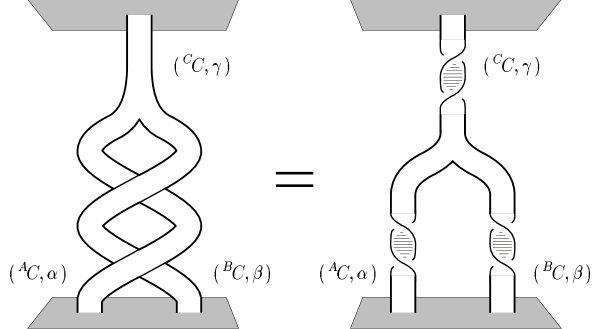
Figure 1.11: Generalized spin-statistics connection. The displayed ribbon diagrams are homotopic as can be checked with the pair of pants you are presently wearing. This means that a monodromy of two particles in a given fusion channel followed by fusion of the pair can be continuously deformed into the process describing a rotation over an angle of $-2\pi$ of the two particles seperately followed by fusion of the pair and a final rotation over an angle of $2\pi$ of the composite.

The analysis for a configuration of two indistinguishable particles $(\,^{A}C,\alpha\,)$ is analogous. The total internal Hilbert space $V_{\alpha}^{A}\otimes V_{\alpha}^{A}$ decomposes into one dimensional irreducible subspaces under the action of the truncated braid group $B(2,m)$ with $m$ the order of the braid operator ${\cal R}$, which depends on the system under consideration. By the same argument as before, the two particle total flux/charge eigenstates spanning a given fusion channel $V_{\gamma}^{C}$ all carry the same one dimensional representation of $B(2,m)$. The quantum statistical parameter assigned to this channel now satisfies the square root version of the generalized spin-statistics connection (1.5.40)

$$K^{AAC}_{\alpha\alpha\gamma}\;{\cal R} = \epsilon\;e^{\pi\imath(s_{(C,\gamma)}-2s_{(A,\alpha)})}\;\;K^{AAC}_{\alpha\alpha\gamma},$$ (1.5.42)

with $\epsilon$ a sign depending on whether the fusion channel $V_{\gamma}^{C}$ appears in a symmetric or an anti-symmetric fashion [14]. In other words, the internal space Hilbert space for a system of two indistinguishable particles $(\,^{A}C,\alpha\,)$ breaks up into the following irreducible representations of the direct product $D(H)\times B(2,m)$

$$\bigoplus_{C,\gamma}N^{AA\gamma}_{\alpha\alpha C}\;(\Pi^{C}_{\gamma},\Lambda_{C-2A}),$$ (1.5.43)

with $\Lambda_{C-2A}$ the one dimensional representation of the truncated braid group $B(2,m)$ defined in (1.5.42).

The result (1.5.42) is actually rather surprising. It states that indistinguishable particle systems in a nonabelian discrete $H$ gauge theory quite generally violate the canonical spin-statistics connection (1.3.40). More accurately, in a nonabelian discrete gauge theory we are dealing with the generalized connection (1.5.42), which incorporates the canonical one. In fact, the canonical spin-statistics connection is retrieved in some particular channels occurring in (1.5.43), as we will argue now. Let us first emphasize that the basic assertions for the ribbon proof depicted in figure 1.7 are naturally satisfied in the nonabelian setting as well. For every particle $(\,^{A}C,\alpha\,)$ in the spectrum there exists an anti-particle $(\,^{\bar{A}}C,\bar{\alpha}\,)$ such that under the proper composition the pair acquires the quantum numbers of the vacuum and may decay. Moreover, every particle carries the same spin as its anti-partner, as indicated by the fact that the charge conjugation operator ${\cal C}$ commutes with the modular matrix $T$. It should be noted now that the ribbon proof in figure 1.7 actually only applies to states in which the particles that propagate along the exchanged ribbons are in strictly identical internal states. Otherwise the ribbons can not be closed. Indeed, we find that the action (1.5.16) of the braid operator on two particles in identical internal flux/charge eigenstates

$${\cal R}\;|\,^{A}\!h_{i},\,^{\alpha}\!v_{j}\rangle|\,^{A}\!h_{i},\,^{\alpha}\!v_{j}\rangle = |\,^{A}\!h_{i},\,\alpha\,(\,^{A}\!h_{1}\,)_{mj}\,^{\alpha}\!v_{j}\rangle|\,^{A}\!h_{i},\,^{\alpha}\!v_{j}\rangle,$$ (1.5.44)

boils down to the diagonal matrix (1.5.11) and therefore to the spin factor (1.5.45) for all $i,j$

$$\exp(\imath\Theta_{(A,\alpha)}) = \exp(2\pi\imath s_{(A,\alpha)}).$$ (1.5.45)

The conclusion is that the canonical spin-statistics connection is restored in the fusion channels spanned by linear combinations of the states (1.5.44) in which the particles are in strictly identical internal flux/charge eigenstates. The quantum statistical parameter (1.5.42) assigned to these channels reduces to the spin factor (1.5.45), thus the effect of a counterclockwise interchange of the two particles in the states in these channels is the same as the effect of rotating one of the particles over an angle of $2\pi$. To conclude, the closed ribbon proof does not apply to the other channels and we are left with the more involved connection (1.5.42) following from the open ribbon argument displayed in figure 1.11.

Finally, higher dimensional irreducible braid group representations are conceivable for a system of more than two particles. The occurrence of such representations simply means that the generators of the braid group can not be diagonalized simultaneously. What happens in this situation is that under the full set of braid operations, the system jumps between isotypical fusion channels, i.e. fusion channels of the same type or ‘color’. Let us make this statement more precise. To keep the discussion general, we do not specify the nature of the particles in the system. Depending on whether the system consists of distinguishable particles, indistinguishable particles or some mixture, we are dealing with a truncated braid group, a colored braid group or a partially colored braid group respectively. The internal Hilbert for such a system again decomposes into a direct sum of irreducible subspaces (or fusion channels) under the action of the quantum double. Given the fact that the action of the associated braid group commutes with that of the quantum double, we are left with two possibilities. First of all, there will in general be some fusion channels separately being invariant under the action of the full braid group. As in the two particle systems discussed before, the total flux/charge eigenstates spanning such a fusion channel, say $V_{\gamma}^{C}$, carry the same one dimensional irreducible representation $\Lambda_{ab}$ of the braid group, that is, these states realize abelian braid statistics with the same quantum statistical parameter. The fusion channel $V_{\gamma}^{C}$ then carries the irreducible representation $(\Pi_{\gamma}^{C},\Lambda_{ab})$ of the direct product of the quantum double and the braid group. In addition, it is also feasible that states carrying the same total flux and charge in different (isotypical) fusion channels are mixed under the action of the full braid group. In that case, we are dealing with a higher dimensional irreducible representation of the truncated braid group or nonabelian braid statistics. Note that nonabelian braid statistics is conceivable, if and only if some fusion channel, say $V_{\delta}^{D}$, occurs more then once in the decomposition of the Hilbert space under the action of the quantum double. Only then there are some orthogonal states with the same total flux and charge available to span an higher dimensional irreducible representation of the braid group. The number $n$ of fusion channels $V_{\delta}^{D}$ related by the action of the braid operators now constitutes the dimension of the irreducible representation $\Lambda_{nonab}$ of the braid group and the multiplicity of this representation is the dimension $d$ of the fusion channel $V_{\delta}^{D}$. To conclude, the direct sum of these $n$ fusion channels $V_{\delta}^{D}$ carries an $n\cdot d$ dimensional irredicible representation $(\Pi_{\delta}^{D},\Lambda_{nonab})$ of the direct product of the quantum double and the braid group.

1.6 $\bar{D}_{2}$ gauge theory

Here, we will illustrate the general considerations of the foregoing sections with one of the simplest nonabelian discrete ${H}$ gauge theories, namely that with gauge group the double dihedral group ${H}\simeq\bar{D}_{2}$, see also [18, 19, 20].

A $\bar{D}_{2}$ gauge theory may, for instance, appear as ‘the long distance remnant’ of a Higgs model of the form (1.4.22) in which the gauge group $G\simeq SU(2)$ is spontaneously broken down to the double dihedral group $H\simeq\bar{D}_{2}\subset SU(2)$. Since $SU(2)$ is simply connected, the fundamental group $\pi_{1}(SU(2)/\bar{D}_{2})$ coincides with the residual symmetry group $\bar{D}_{2}$. Hence, the stable magnetic fluxes in this broken theory are indeed labeled by the group elements of $\bar{D}_{2}$. See the discussion concerning the isomorphism (1.4.3) in section 1.4.1. In the following, we will not dwell any further on the explicit details of this or other possible embeddings in broken gauge theories and simply focus on the features of the $\bar{D}_{2}$ gauge theory itself. We start with a discussion of the spectrum.

Conjugacy class		Centralizer
$e=\{e\}$		$\qquad\bar{D}_{2}$
$\bar{e}=\{\bar{e}\}$		$\qquad\bar{D}_{2}$
$X_{1}=\{X_{1},\bar{X}_{1}\}\$		$\qquad{\mbox{\bf Z}}_{4}\simeq\{e,X_{1},\bar{e},\bar{X}_{1}\}$
$X_{2}=\{X_{2},\bar{X}_{2}\}$		$\qquad{\mbox{\bf Z}}_{4}\simeq\{e,X_{2},\bar{e},\bar{X}_{2}\}$
$X_{3}=\{X_{3},\bar{X}_{3}\}$		$\qquad{\mbox{\bf Z}}_{4}\simeq\{e,X_{3},\bar{e},\bar{X}_{3}\}$

Table 1.1: Conjugacy classes of $\bar{D}_{2}$ together with their centralizers.

$\rule{0.0pt}{9.95845pt}\bar{D}_{2}\qquad$	$e$	$\bar{e}$	$X_{1}$	$X_{2}$	$X_{3}$
$1\rule{0.0pt}{9.95845pt}$	$1$	$1$	$1$	$1$	$1$
$J_{1}\rule{0.0pt}{9.95845pt}$	$1$	$1$	$1$	$-1$	$-1$
$J_{2}\rule{0.0pt}{9.95845pt}$	$1$	$1$	$-1$	$1$	$-1$
$J_{3}\rule{0.0pt}{9.95845pt}$	$1$	$1$	$-1$	$-1$	$1$
$\chi\rule{0.0pt}{9.95845pt}$	$2$	$-2$	$0$	$0$	$0$

$\rule{0.0pt}{9.95845pt}{\mbox{\bf Z}}_{4}\qquad$	$e$	$X_{a}$	$\bar{e}$	$\bar{X}_{a}$
${\Gamma^{0}}\rule{0.0pt}{9.95845pt}$	$1$	$1$	$1$	$1$
${\Gamma^{1}}\rule{0.0pt}{9.95845pt}$	$1$	$\imath$	$-1$	$-\imath$
${\Gamma^{2}}\rule{0.0pt}{9.95845pt}$	$1$	$-1$	$1$	$-1$
${\Gamma^{3}}\rule{0.0pt}{9.95845pt}$	$1$	$-\imath$	$-1$	$\imath$

Table 1.2: Character tables of $\bar{D}_{2}$ and ${\mbox{\bf Z}}_{4}$.

The double dihedral group $\bar{D}_{2}$ is a group of order $8$ with a nontrivial centre of order $2$. The fluxes associated with its group elements are organized in the conjugacy classes exhibited in table 1.1. There are five conjugacy classes denoted by $e,\bar{e},X_{1},X_{2}$ and $X_{3}$. The conjugacy class $e$ corresponds to the trivial flux sector, while $\bar{e}$ contains the nontrivial centre element. The conjugacy classes $X_{1},X_{2}$ and $X_{3}$ consist of two commuting elements of order $4$. Thus there are four nontrivial purely magnetic flux sectors: one singlet flux $\bar{e}$ and three different doublet fluxes $X_{1},X_{2}$ and $X_{3}$. The purely electric charge sectors, on the other hand, correspond to the UIR’s of $\bar{D}_{2}$. From the character table displayed in table 1.2, we infer that there are four nontrivial pure charges in the spectrum: three singlet charges $J_{1},J_{2},J_{3}$ and one doublet charge $\chi$. The fluxes $X_{a}/\bar{X}_{a}$ act on the doublet charge $\chi$ as $\pm\imath\sigma_{a}$, with $\sigma_{a}$ being the Pauli matrices. Let us now turn to the dyonic sectors. These are constructed by assigning nontrivial centralizer representation to the nontrivial fluxes. The centralizers associated with the different flux sectors can be found in table 1.1. The flux $\bar{e}$ obviously commutes with the full group $\bar{D}_{2}$, while the centralizer of the other flux sectors is the cyclic group ${\mbox{\bf Z}}_{4}$. Thus we arrive at thirteen different dyons: three singlet dyons and one doublet dyon associated with the flux $\bar{e}$ and nine doublets dyons associated with the fluxes $X_{1},X_{2}$ and $X_{3}$ paired with nontrivial ${\mbox{\bf Z}}_{4}$ representations. All in all, the spectrum of this theory features 22 particles, which will be labeled as

$$\begin{array}[]{rclrcl}1&:=&(e,\,1)&\qquad\qquad\bar{1}&:=&(\bar{e},\,1)\\ J_{a}&:=&(e,\,J_{a})&\qquad\qquad\bar{J}_{a}&:=&(\bar{e},\,J_{a})\\ \chi&:=&(e,\,\chi)&\qquad\qquad\bar{\chi}&:=&(\bar{e},\,\chi)\\ \sigma_{a}^{+}&:=&(X_{a},\,{\Gamma^{0}})&\qquad\qquad\sigma_{a}^{-}&:=&(X_{a},\,{\Gamma^{2}})\\ \tau_{a}^{+}&:=&(X_{a},\,{\Gamma^{1}})&\qquad\qquad\tau_{a}^{-}&:=&(X_{a},\,{\Gamma^{3}}),\end{array}$$ (1.6.6)

for convenience. Note that the square of the dimensions of the internal Hilbert spaces carried by these particles indeed add up to the order of the quantum double $D(\bar{D}_{2})$: $8\cdot 1^{2}+14\cdot 2^{2}=8^{2}$.

We proceed with a detailed analysis of the topological interactions between the particles in the spectrum (1.6.6). The discussion is organized as follows. In section 1.6.1, we will establish the fusion rules. This is the natural setting to discuss a feature special for nonabelian discrete ${H}$ gauge theories: a pair of nonabelian fluxes can carry charges that are not localized on any of the two fluxes nor anywhere else. We will show that these so-called Cheshire charges can be excited by monodromy processes with for instance the doublet charges $\chi$. To proceed, section 1.6.2 contains a discussion of the cross sections associated with Aharonov-Bohm scattering experiments with the particles in this theory. Finally, the issue of nonabelian braid statistics will be dealt with in section 1.6.3.

1.6.1 Alice in physics

As we have seen in section 1.5.3, the topological interactions for a particular discrete ${H}$ gauge theory are classified by the content of the associated modular matrices $S$ and $T$. The modular $T$ matrix (1.5.38) contains the spin factors of the particles. For the particles in the spectrum of this $\bar{D}_{2}$ gauge theory we easily infer

$$\begin{array}[]{cc}\mbox{particle}&\qquad\exp(2\pi\imath s)\\ 1,J_{a}&\qquad 1\\ \bar{1},\bar{J}_{a}&\qquad 1\\ \chi/\bar{\chi}&\qquad\pm 1\\ \sigma_{a}^{\pm}&\qquad\pm 1\\ \tau_{a}^{\pm}&\qquad\pm\imath.\end{array}$$ (1.6.13)

The modular $S$ matrix (1.5.3), on the other hand, is determined by the monodromy matrix following from (1.5.16). It can be verified that the modular $S$ matrix for this model is real and therefore orthogonal. For future reference, we have displayed it in table 1.3. In this section, we will focus on the fusion rules obtained from Verlinde’s formula (1.5.37) and the key role they play as overall selection rules for the flux/charge exchanges occurring when the particles encircle each other.

$S$		$1$	$\bar{1}$	$J_{a}$	$\bar{J}_{a}$	$\chi$	$\bar{\chi}$	$\sigma^{+}_{a}$	$\sigma^{-}_{a}$	$\tau^{+}_{a}$	$\tau^{-}_{a}$
$1$		$1$	$1$	$1$	$1$	$2$	$2$	$2$	$2$	$2$	$2$
$\bar{1}$		$1$	$1$	$1$	$1$	$-2$	$-2$	$2$	$2$	$-2$	$-2$
$J_{b}$		$1$	$1$	$1$	$1$	$2$	$2$	$2\epsilon_{ab}$	$2\epsilon_{ab}$	$2\epsilon_{ab}$	$2\epsilon_{ab}$
$\bar{J}_{b}$		$1$	$1$	$1$	$1$	$-2$	$-2$	$2\epsilon_{ab}$	$2\epsilon_{ab}$	$-2\epsilon_{ab}$	$-2\epsilon_{ab}$
$\chi$		$2$	$-2$	$2$	$-2$	$4$	$-4$	$0$	$0$	$0$	$0$
$\bar{\chi}$		$2$	$-2$	$2$	$-2$	$-4$	$4$	$0$	$0$	$0$	$0$
$\sigma^{+}_{b}$		$2$	$2$	$2\epsilon_{ab}$	$2\epsilon_{ab}$	$0$	$0$	$4\delta_{ab}$	$-4\delta_{ab}$	$0$	$0$
$\sigma^{-}_{b}$		$2$	$2$	$2\epsilon_{ab}$	$2\epsilon_{ab}$	$0$	$0$	$-4\delta_{ab}$	$4\delta_{ab}$	$0$	$0$
$\tau^{+}_{b}$		$2$	$-2$	$2\epsilon_{ab}$	$-2\epsilon_{ab}$	$0$	$0$	$0$	$0$	$-4\delta_{ab}$	$4\delta_{ab}$
$\tau^{-}_{b}$		$2$	$-2$	$2\epsilon_{ab}$	$-2\epsilon_{ab}$	$0$	$0$	$0$	$0$	$4\delta_{ab}$	$-4\delta_{ab}$

Table 1.3: Modular S-matrix of the quantum double $D(\bar{D}_{2})$ up to an overall factor $\frac{1}{8}$. We defined $\epsilon_{ab}=1$ if $a=b$ and $-1$ otherwise.

We start with the fusion rules for the purely electric charges. These are dictated by the representation ring of $\bar{D}_{2}$

$$J_{a}\times J_{a}=1,\qquad J_{a}\times J_{b}=J_{c},\qquad J_{a}\times\chi=\chi,\qquad\chi\times\chi=1+\sum_{a}J_{a}.$$ (1.6.14)

The dyons associated with the flux $\bar{1}$ are obtained by simply composing this flux with the purely electric charges

$$J_{a}\times\bar{1}=\bar{J}_{a},\qquad\chi\times\bar{1}=\bar{\chi}.$$ (1.6.15)

In a similar fashion, we produce the other dyons

$$J_{a}\times\sigma^{+}_{a}=\sigma^{+}_{a},\qquad J_{b}\times\sigma^{+}_{a}=\sigma^{-}_{a},\qquad\chi\times\sigma^{+}_{a}=\tau^{+}_{a}+\tau^{-}_{a}.$$ (1.6.16)

We now have all the constituents of the spectrum (1.6.6). Recall that the fusion algebra is commutative and associative. This implies that the complete set of fusion rules is actually determined by a minimal subset. Bearing this in mind, amalgamation involving the flux $\bar{1}$ is unambiguously prescribed by (1.6.15) and

$$\bar{1}\times\bar{1}=1,\qquad\bar{1}\times\sigma^{\pm}_{a}=\sigma^{\pm}_{a},\qquad\bar{1}\times\tau^{\pm}_{a}=\tau^{\mp}_{a}.$$ (1.6.17)

The complete set of fusion rules is fixed by the previous ones together with

$$J_{a}\times\tau^{\pm}_{a}=\tau^{\pm}_{a},\qquad J_{b}\times\tau^{\pm}_{a}=\tau^{\mp}_{a},\qquad\chi\times\tau^{\pm}_{a}=\sigma^{+}_{a}+\sigma^{-}_{a},$$ (1.6.18)

and

$$\sigma^{\pm}_{a}\times\sigma^{\pm}_{a} = 1+J_{a}+\bar{1}+\bar{J}_{a}$$ (1.6.19)

$$\sigma^{\pm}_{a}\times\sigma^{\pm}_{b} = \sigma^{+}_{c}+\sigma^{-}_{c}$$ (1.6.20)

$$\sigma^{\pm}_{a}\times\tau^{\pm}_{a} = \chi+\bar{\chi}$$ (1.6.21)

$$\sigma^{\pm}_{a}\times\tau^{\pm}_{b} = \tau^{+}_{c}+\tau^{-}_{c}$$ (1.6.22)

$$\tau^{\pm}_{a}\times\tau^{\pm}_{a} = 1+J_{a}+\bar{J}_{b}+\bar{J}_{c}$$ (1.6.23)

$$\tau^{\pm}_{a}\times\tau^{\pm}_{b} = \sigma^{+}_{c}+\sigma^{-}_{c}.$$ (1.6.24)

A few remarks are pertinent at this stage. First of all, the class algebra of $\bar{D}_{2}$ is respected as an overall selection rule. The class multiplication in the fusion rule (1.6.19), for instance, reads $X_{a}*X_{a}=2e+2\bar{e}$. The appearance of the class algebra expresses magnetic flux conservation. In establishing the fusion rule, all fluxes in the consecutive conjugacy classes are multiplied out. To proceed, the modular $S$ matrix as given in table 1.3 is real and therefore equal to its inverse as follows from (1.5.3). As a consequence, the charge conjugation operator ${\cal C}$ acts on the spectrum (1.6.6) as the unit matrix ${\cal C}=S^{2}={\mbox{\bf 1}}$, thus the particles in this $\bar{D}_{2}$ gauge theory feature as their own anti-partner. Only two similar particles are able to annihilate, as witnessed by the occurrence of the vacuum representation $1$ in the fusion rule for two similar particles.

At first sight, the message of the fusion rule (1.6.19) is rather remarkable. It seems that the fusion of two pure fluxes $\sigma_{a}^{+}$ may give rise to electric charge creation. One could start wondering about electric charge conservation at this point. Electric charge is conserved though. Before fusion this charge was present in the form of so-called nonlocalizable Cheshire charge [107, 5, 18, 20], i.e. the nontrivial representation of the global symmetry group $\bar{D}_{2}$ carried by the pair. This becomes clear upon writing the fusion rule (1.6.19) in terms of the two particle flux states for the different channels

$$\frac{1}{\sqrt{2}}\{|\bar{X}_{a}\rangle|X_{a}\rangle\;+\;|X_{a}\rangle|\bar{X}_{a}\rangle\} \longmapsto 1$$ (1.6.25)

$$\frac{1}{\sqrt{2}}\{|\bar{X}_{a}\rangle|X_{a}\rangle\;-\;|X_{a}\rangle|\bar{X}_{a}\rangle\} \longmapsto J_{a}$$ (1.6.26)

$$\frac{1}{\sqrt{2}}\{|X_{a}\rangle|X_{a}\rangle\;+\;|\bar{X}_{a}\rangle|\bar{X}_{a}\rangle\} \longmapsto \bar{1}$$ (1.6.27)

$$\frac{1}{\sqrt{2}}\{|X_{a}\rangle|X_{a}\rangle\;-\;|\bar{X}_{a}\rangle|\bar{X}_{a}\rangle\} \longmapsto \bar{J}_{a}.$$ (1.6.28)

The identification of the two particle flux states with the single particle states is established by the action (1.5.12) of the quantum double $D(\bar{D}_{2})$ on these two particle states. On the one hand, we can perform global $\bar{D}_{2}$ symmetry transformations from which we learn the charge carried by the flux pair. As indicated by the comultiplication (1.5.12), these act as an overall conjugation. The total flux of the pair, on the other hand, is obtained by applying the flux projection operators (1.5.1). Note that the above quantum states describing the flux pairs are nonseparable. The two fluxes are correlated: by measuring the flux of one particle of the pair we instantaneously fix the flux of the other. This is the famous Einstein-Podolsky-Rosen (EPR) paradox [54]. It is no longer possible to make a flux measurement on one particle without affecting the other instantaneously, just as in the notorious experiment with two spin $1/2$ particles in the singlet state. The Cheshire charge carried by the flux pair depends on the symmetry properties of these nonseparable quantum states. The symmetric quantum states correspond to the trivial charge $1$, whereas the anti-symmetric quantum states carry the nontrivial charge $J_{a}$. It is clear that the charge $J_{a}$ can not be localized on any of the fluxes nor anywhere else. It is a property of the pair and only becomes localized when the fluxes are brought together in a fusion process. It is this elusive nature, reminiscent of the smile of the Cheshire cat in Alice’s adventures in wonderland [40], that was the motivation to call such a charge Cheshire charge.

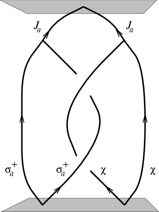
Figure 1.12: A charge/anti-charge pair $\chi$ and a flux/anti-flux pair $\sigma_{a}^{+}$ are created from the vacuum at a certain time slice. The lines denote the worldlines of the particles. After the charge $\chi$ has encircled the flux $\sigma_{a}^{+}$, both particle/anti-particle pairs carry Cheshire charge $J_{a}$. These Cheshire charges become localized upon bringing the members of the pairs together again. Subsequently, the two charges $J_{a}$ annihilate.

The Cheshire charge $J_{a}$ of the flux pair can be excited by encircling one flux in the pair by the doublet charge $\chi$ [107, 20, 8]. Here we draw on a further analogy with Alice’s adventures. The magnetic fluxes $\{X_{a},\bar{X}_{a}\}$ act by means of the Pauli matrices $\pm\imath\sigma_{a}$ on the doublet charge $\chi$. This means that when a charge $\chi$ with its orientation down is adiabatically transported around, for example, the flux $X_{2}$, it returns with its orientation up

$${\cal R}^{2}\;|X_{2}\rangle|\left(\begin{array}[]{c}0\\ 1\end{array}\right)\rangle = |X_{2}\rangle|\left(\begin{array}[]{c}1\\ 0\end{array}\right)\rangle,$$ (1.6.33)

as follows from (1.5.16). In terms of Alice’s adventures: the charge has gone through the looking-glass. For this reason the flux $X_{2}$ is called an Alice flux [116, 5, 107]. The other fluxes $X_{a},\bar{X}_{a}$ affect the doublet charge $\chi$ in a similar way. Now consider the process depicted in figure 1.12. We start with the creation of a charge/anti-charge pair $\chi$ and a flux/anti-flux pair $\sigma_{a}^{+}$ from the vacuum. Thus both pairs do not carry Cheshire charge at this stage. They are in the vacuum channel of the corresponding fusion rules (1.6.14) and (1.6.19). Next, one member of the charge pair encircles a flux in the flux pair. The flip of the charge orientation (1.6.33) leads to an exchange of the internal quantum numbers of the pairs: both pairs carry Cheshire charge $J_{a}$ after this process, i.e. both pairs are in the $J_{a}$ channel of the associated fusion rules. The global charge of the configuration is conserved. Both charges $J_{a}$ can be annihilated by bringing them together as follows from the fusion rules (1.6.14). These phenomena can be made explicit by writing this process in terms of the corresponding correlated internal quantum states

$$1 \longmapsto \frac{1}{2}\{|\bar{X}_{2}\rangle|X_{2}\rangle\;+\;|X_{2}\rangle|\bar{X}_{2}\rangle\}\{|\left(\begin{array}[]{c}1\\ 0\end{array}\right)\rangle|\left(\begin{array}[]{c}0\\ 1\end{array}\right)\rangle\;-\;|\left(\begin{array}[]{c}0\\ 1\end{array}\right)\rangle|\left(\begin{array}[]{c}1\\ 0\end{array}\right)\rangle\}$$ (1.6.42)

$$\stackrel{{\scriptstyle{\mbox{\scriptsize\bf 1}}\otimes{\cal R}^{2}\otimes{\mbox{\scriptsize\bf 1}}}}{{\longmapsto}} \frac{1}{2}\{|\bar{X}_{2}\rangle|X_{2}\rangle\;-\;|X_{2}\rangle|\bar{X}_{2}\rangle\}\{|\left(\begin{array}[]{c}0\\ 1\end{array}\right)\rangle|\left(\begin{array}[]{c}0\\ 1\end{array}\right)\rangle\;+\;|\left(\begin{array}[]{c}1\\ 0\end{array}\right)\rangle|\left(\begin{array}[]{c}1\\ 0\end{array}\right)\rangle\}$$

$$\longmapsto |J_{2}\rangle|J_{2}\rangle$$

$$\longmapsto 1.$$ (1.6.52)

Here we used (1.5.16) and the fact that the fluxes $\{X_{2},\bar{X}_{2}\}$ act by means of the Pauli matrices $\pm\imath\sigma_{2}$ on the charge $\chi$. After the charge has encircled the flux, the flux pair is in the anti-symmetric quantum state (1.6.26) with Cheshire charge $J_{2}$, while the same observation holds for the quantum state of the charge pair. Before fusion the charge pair was in the anti-symmetric vacuum representation $1$, while the state that emerges after the monodromy carries the Cheshire charge $J_{2}$. For convenience, we restricted ourselves to the flux pair $\sigma_{2}^{+}$ here. The argument for the other flux pairs is completely similar.

This discussion naturally extends to the exchange of magnetic quantum numbers in monodromy processes involving noncommuting fluxes (1.4.19). If we replace the doublet charge pair by a flux pair $\sigma_{b}^{+}$ starting off in the vacuum channel (1.6.25), both flux pairs end up in the nontrivial flux channel (1.6.27) after the monodromy and both pairs now carry the total flux $\bar{1}$. These fluxes become localized upon fusing the members of the pairs, and subsequently annihilate each other according to their fusion rule (1.6.17).

We close this section by emphasizing the profound role that the fusion rules play as overall selection rules in the flux/charge exchange processes among the particles. It is natural to confine our considerations to multi-particle systems which are in the vacuum sector $1$, i.e. the overall flux and charge of this system vanishes. Thus the particles necessarily appear in pairs, as we have seen in the example of such a system in figure 1.12. The fusion rules classify the different total fluxes and Cheshire charges these pairs can carry and determine the flux/charge exchanges that may occur in monodromy processes involving particles in different pairs.

1.6.2 Scattering doublet charges off Alice fluxes

The Aharonov-Bohm interactions among the particles in the spectrum (1.6.6) roughly fall into two classes. First of all there are the interactions in which no internal flux/charge quantum numbers are exchanged between the particles. In this case, the monodromy matrix following from (1.5.16) is diagonal in the two particle flux/charge eigenbasis, with possibly different Aharonov-Bohm phases as diagonal elements. The cross sections measured in Aharonov-Bohm scattering experiments with the associated particles simply follow from the well-known cross section (1.A.2) derived by Aharonov and Bohm [4]. The more interesting Aharonov-Bohm interactions are those in which internal flux/charge quantum numbers are exchanged between the particles. In this case, the monodromy matrix is off diagonal in the flux/charge eigenbasis. The cross sections appearing in Aharonov-Bohm scattering experiments involving such particles are discussed in appendix 1.A. In this section, we will focus on a nontrivial example, namely an Aharonov-Bohm experiment in which a doublet charge $\chi$ scatters from an Alice flux $\sigma_{2}^{+}$.

The total internal Hilbert space associated with the two particle system consisting of a pure doublet charge $\chi$ together with a pure doublet flux $\sigma_{2}^{+}$ is four dimensional. We define the following natural flux/charge eigenbasis in this internal Hilbert space

$$\begin{array}[]{rclrcl}e_{\uparrow\uparrow}&=&|X_{2}\rangle|\left(\begin{array}[]{c}1\\ 0\end{array}\right)\rangle\\ e_{\uparrow\downarrow}&=&|X_{2}\rangle|\left(\begin{array}[]{c}0\\ 1\end{array}\right)\rangle\\ e_{\downarrow\uparrow}&=&|\bar{X}_{2}\rangle|\left(\begin{array}[]{c}1\\ 0\end{array}\right)\rangle\\ e_{\downarrow\downarrow}&=&|\bar{X}_{2}\rangle|\left(\begin{array}[]{c}0\\ 1\end{array}\right)\rangle.\end{array}$$ (1.6.65)

The fluxes ${X}_{2}/\bar{X}_{2}$ are represented by the Pauli matrices $\pm\imath\sigma_{2}$ in the doublet charge representation $\chi$. From (1.5.16), we then infer that the monodromy matrix takes the following block diagonal in this basis

$${\cal R}^{2} = \left(\begin{array}[]{rrrr}0&1&&\\ -1&0&&\\ &&0&-1\\ &&1&0\end{array}\right),$$ (1.6.70)

which summarizes the phenomenon discussed in the previous section: the orientation of the charge $\chi$ is flipped, when it is transported around the Alice fluxes ${X}_{2}$ or $\bar{X}_{2}$.

Let us now consider the Aharonov-Bohm scattering experiment in which the doublet charge $\chi$ scatters from the Alice flux $\sigma_{2}^{+}$. We assume that we are measuring with a detector that only gives a signal when a scattered charge $\chi$ enters the device with a specific orientation (either $\uparrow$ or $\downarrow$). Here we may, for instance, think of an apparatus in which we have captured the associated anti-particle. This is the charge with opposite orientation, as we have seen in (1.6.42). If the orientation of the scattered charge entering the device matches that of the anti-particle, the pair annihilates and we assume that the apparatus somehow gives a signal when such an annihilation process occurs. The cross section measured with such a detector involves the matrix elements of the scattering matrix

$${\cal R}^{-\theta/\pi}({\mbox{\bf 1}}-{\cal R}^{2}) = \sqrt{2}e^{-\imath\theta/2}\left(\begin{array}[]{rrrr}\cos{\frac{\pi-\theta}{4}}&\sin{\frac{\pi-\theta}{4}}&&\\ -\sin{\frac{\pi-\theta}{4}}&\cos{\frac{\pi-\theta}{4}}&&\\ &&\cos{\frac{\pi-\theta}{4}}&-\sin{\frac{\pi-\theta}{4}}\\ &&\sin{\frac{\pi-\theta}{4}}&\cos{\frac{\pi-\theta}{4}}\end{array}\right).$$

for the flux/charge eigenstates (1.6.65). This scattering matrix is determined using the prescription (1.A.5) in the monodromy eigenbasis in which the above monodromy matrix (1.6.70) is diagonal, and subsequently transforming back to the flux/charge eigenbasis (1.6.65). Now suppose that the scatterer is in a particular flux eigenstate, while the projectile that comes in is a charge with a specific orientation and the detector is only sensitive for scattered charges with this specific orientation. Under these circumstances, the two particle in and out state are the same, $|\,\mbox{in}\rangle=|\,\mbox{out}\rangle$, and equal to one of the flux/charge eigenstates in (1.6.65). In other words, we are measuring the scattering amplitudes on the diagonal of the scattering matrix (1.6.2). Note that the formal sum of the out state $|\mbox{out}\rangle$ over a complete basis of flux eigenstates for the scatterer, as indicated in appendix 1.A, boils down to one term here, namely the flux eigenstate of the scatterer in the in state $|\mbox{in}\rangle$. The other flux eigenstate does not contribute. The corresponding matrix element vanishes, because the flux of the scatterer is not affected when it is encircled by the charge $\chi$. From (1.A.4) we obtain the following exclusive cross section for this scattering experiment

$$\frac{{\rm d}\sigma_{+}}{{\rm d}\theta} = \frac{1+\sin{(\theta/2)}}{8\pi p\sin^{2}{(\theta/2)}}\;.$$ (1.6.72)

The charge flip cross section, in turn, is measured by a detector which only signals scattered charges with an orientation opposite to the orientation of the charge of the projectile. In this case, the state $|\mbox{in}\rangle$ is again one of the flux/charge eigenstates in (1.6.65), while the $|\mbox{out}\rangle$ state we measure is the same as the in state, but with the orientation of the charge flipped. Thus we are now measuring the off diagonal matrix elements of the scattering matrix (1.6.2). In a similar fashion as before, we find the following form for the charge flip cross section

$$\frac{{\rm d}\sigma_{-}}{{\rm d}\theta} = \frac{1-\sin{(\theta/2)}}{8\pi p\sin^{2}{(\theta/2)}}\;.$$ (1.6.73)

The exclusive cross sections (1.6.72) and (1.6.73), which are the same as derived for scattering of electric charges from Alice fluxes in Alice electrodynamics by Lo and Preskill [92], are clearly multi-valued

$$\frac{{\rm d}\sigma_{\pm}}{{\rm d}\theta}\;(\theta+2\pi) = \frac{{\rm d}\sigma_{\mp}}{{\rm d}\theta}\;(\theta).$$ (1.6.74)

This merely reflects the fact that a detector only signalling charges $\chi$ with their orientation up, becomes a detector only signalling charges with orientation down (and vice versa), when it is transported over an angle $2\pi$ around the scatterer. Specifically, in this parallel transport the anti-particle in our detector feels the holonomy in the gauge fields associated with the flux of the scatterer and returns with its orientation flipped. As a consequence, the device becomes sensitive for the opposite charge orientation after this parallel transport.

Verlinde’s detector does not suffer from this multi-valuedness. It does not discriminate between the orientations of the scattered charge, and gives a signal whenever a charge $\chi$ enters the device. This detector measures the total or inclusive cross section, i.e. both branches of the multi-valued cross section (1.6.72) (or (1.6.73) for that matter). To be specific, the exclusive cross sections (1.6.72) and (1.6.73) combine in the following fashion

$$\frac{{\rm d}\sigma}{{\rm d}\theta}\;=\;\frac{{\rm d}\sigma_{-}}{{\rm d}\theta}+\frac{{\rm d}\sigma_{+}}{{\rm d}\theta}\;=\;\frac{1}{4\pi p\sin^{2}{(\theta/2)}}\;.$$ (1.6.75)

into Verlinde’s single valued inclusive cross section (1.A.3) for this scattering experiment.

The above analysis is easily extended to Aharonov-Bohm scattering experiments involving other particles in the spectrum (1.6.6) of this $\bar{D}_{2}$ gauge theory. It should be stressed however, that a crucial ingredient in the derivation of the multi-valued exclusive cross sections (1.6.72) and (1.6.73) is that the monodromy matrix (1.6.70) is off diagonal and has imaginary eigenvalues $\pm\imath$. In the other cases, where the monodromy matrices are diagonal or off diagonal with eigenvalues $\pm 1$, as it appears for scattering noncommuting fluxes $\sigma_{a}^{+}$ and $\sigma_{b}^{+}$ from each other, we arrive at single valued exclusive cross sections.

1.6.3 Nonabelian braid statistics

We finally turn to the issue of nonabelian braid statistics. As we have argued in section 1.5.2, the braidings and monodromies for multi-particle configurations appearing in discrete ${H}$ gauge theories are governed by truncated braid groups. To be precise, the total internal Hilbert space for a given multi-particle system carries a representation of some truncated braid group, which in general decomposes into a direct sum of irreducible representations. In this section, we identify the truncated braid groups ruling in this particular $\bar{D}_{2}$ gauge theory and elaborate on the aforementioned decomposition. We first consider the indistinguishable particle configurations in this model.

It can easily be verified that the braid operators acting on a configuration, which only contains singlet charges $J_{a}$, are of order one. The same holds for the singlet dyons $\bar{1}$ and $\bar{J}_{a}$. In other words, these particles behave as ordinary bosons, in accordance with the trivial spin factors (1.6.13) assigned to them. To proceed, the braid operators acting on a system of $n$ doublet charges $\chi$ are of order two and therefore realize a (higher dimensional) representation of the permutation group $S_{n}$. The same observation appears for the doublet dyons $\bar{\chi}$ and $\sigma^{\pm}_{a}$. The total internal Hilbert spaces for these indistinguishable particle systems can then be decomposed into a direct sum of subspaces, each carrying an irreducible representation of the permutation group. The one dimensional representations that appear in this decomposition correspond to Bose or Fermi statistics, while the higher dimensional representations describe parastatistics. Finally, braid statistics occurs for a system consisting of $n$ dyons $\tau_{a}^{\pm}$. The braid operators that act on such a system are of order four, thus the associated internal Hilbert space splits up into a direct sum of irreducible representations of the truncated braid group $B(n,4)$. The one dimensional representations that occur in this decomposition realize abelian anyon statistics, whereas the higher dimensional representations correspond to nonabelian braid statistics or nonabelian anyons. We will illustrate these features with two representative examples. We first examine a system containing two dyons $\tau_{1}^{+}$. The irreducible braid group representations available for this system are one dimensional, since the truncated braid group $B(2,4)$ for two particles is abelian. We then turn to the more interesting system consisting of three dyons $\tau_{1}^{+}$. In this case, we are dealing with nonabelian braid statistics. The associated total internal Hilbert space breaks up into four 1-dimensional irreducible subspaces and two 2-dimensional irreducible subspaces under the action of the nonabelian truncated braid group $B(3,4)$.

We start by setting some conventions. First of all, the two fluxes in the conjugacy class associated with the dyon $\tau_{1}^{+}$ are ordered as indicated in table 1.1

$${}^{1}h_{1} = X_{1}$$

$${}^{1}h_{2} = \bar{X}_{1},$$

while we take the following coset representatives appearing in the definition (1.5.7) of the centralizer charge

$${}^{1}x_{1} = e$$

$${}^{1}x_{2} = X_{2}.$$

To lighten the notation a bit, we furthermore use the following abbreviation for the internal flux/charge eigenstates of the dyon $\tau_{1}^{+}$

$$|\uparrow\,\rangle := |X_{1},^{1}v\rangle$$

$$|\downarrow\,\rangle := |\bar{X}_{1},^{1}v\rangle.$$

Let us now consider a system consisting of two dyons $\tau^{+}_{1}$. Under the action of the quantum double $D(\bar{D}_{2})$, the internal Hilbert space $V_{\tau^{+}_{1}}\otimes V_{\tau^{+}_{1}}$ associated with this system decomposes according to the fusion rule (1.6.23), which we repeat for convenience

$$\tau^{+}_{1}\times\tau^{+}_{1} = 1+J_{1}+\bar{J}_{2}+\bar{J}_{3}.$$ (1.6.76)

The two particle states corresponding to the different fusion channels carry an one dimensional (irreducible) representation of the abelian truncated braid group $B(2,4)={\mbox{\bf Z}}_{4}$. We first establish the different irreducible pieces contained in the $B(2,4)$ representation carried by the total internal Hilbert space $V_{\tau^{+}_{1}}\otimes V_{\tau^{+}_{1}}$. This can be done by calculating the traces of the elements $\{e,\tau,\tau^{2},\tau^{3}\}$ of $B(2,4)$ in this representation using the standard diagrammatic techniques (see for instance [79, 2]). From the character vector obtained in this way, we learn that this representation breaks up as

$$\Lambda_{B(2,4)} = 3\;\Gamma^{1}+\Gamma^{3},$$ (1.6.77)

with $\Gamma^{1}$ and $\Gamma^{3}$ the irreducible ${\mbox{\bf Z}}_{4}$ representations displayed in the character table 1.1. After some algebra, we then arrive at the following basis of mutual eigenstates under the combined action of the quantum double and the truncated braid group

$$\halign to=0.0pt{\hskip\@centering$\displaystyle{#}$\@eqnsel&\global\@eqcnt\@ne\hskip\tw@\arraycolsep\hfil${#}$\hfil&\global\@eqcnt\tw@\hskip\tw@\arraycolsep$\displaystyle{#}$\hfil&\global\@eqcnt\thr@@\hskip\tw@\arraycolsep\hfil\hbox{#}&\global\@eqcnt 4 \hbox\bgroup\hss#\egroup\cr 0.0pt plus 1000.0pt$\displaystyle{V_{\tau^{+}_{1}} \otimes V_{\tau^{+}_{1}} \qquad&10.0pt\hfil${\qquad&10.0pt$\displaystyle{D(\bar{D}_{2}) &10.0pt\hfil\hbox{$\qquad B(2,4)$ \\ \frac{1}{\sqrt{2}} \{ |\uparrow\, \rangle|\downarrow\, \rangle-|\downarrow\, \rangle|\uparrow\, \rangle\} &{\hss\qquad}&\;\;1&$\qquad\Gamma^{1} \;\;\; \,$\\\frac{1}{\sqrt{2}}\{|\uparrow\,\rangle|\downarrow\,\rangle+|\downarrow\,\rangle|\uparrow\,\rangle\}&&\;\;J_{1}&$\qquad\Gamma^{3} \;\;\;\,$\\\frac{1}{\sqrt{2}}\{|\uparrow\,\rangle|\uparrow\,\rangle+|\downarrow\,\rangle|\downarrow\,\rangle\}&&\;\;\bar{J}_{2}&$\qquad\Gamma^{1} \;\;\;\, $\\\frac{1}{\sqrt{2}}\{|\uparrow\,\rangle|\uparrow\,\rangle-|\downarrow\,\rangle|\downarrow\,\rangle\}&&\;\;\bar{J}_{3}&$\qquad\Gamma^{1} , \;\;\; $(1.6.78)\cr}}}}}$$

from which we conclude that the two particle internal Hilbert space $V_{\tau^{+}_{1}}\otimes V_{\tau^{+}_{1}}$ decomposes into the following direct sum of one dimensional irreducible representations of the direct product $D(\bar{D}_{2})\times B(2,4)$

$$(1,\Gamma^{1})\>+\>(J_{1},\Gamma^{3})\>+\>(\bar{J}_{2},\Gamma^{1})\>+\>(\bar{J}_{3},\Gamma^{1}).$$ (1.6.79)

The two particle states contained in (1.6.3) and (1.6.3) satisfy the canonical spin-statistics connection (1.5.45), that is, $\exp(\imath\Theta)=\exp(2\pi\imath s_{\tau^{+}_{1}})=\imath$. In other words, these states realize semion statistics. Accidentally, the same observation appears for the state (1.6.3). Finally, the two particle state displayed in (1.6.3) satisfies the generalized spin-statistics connection (1.5.42) and describes semion statistics with quantum statistical parameter $\exp(\imath\Theta)=-\imath$.

We now extend our analysis to a system containing three dyons $\tau^{+}_{1}$. From (1.6.76) and the fusion rules (1.6.15), (1.6.16) and (1.6.17), we infer that the decomposition of the total internal Hilbert space under the action of the quantum double becomes

$$\tau^{+}_{1}\times\tau^{+}_{1}\times\tau^{+}_{1} = 4\;\tau^{+}_{1}.$$ (1.6.80)

The occurrence of four equivalent fusion channels indicates that nonabelian braid statistics is conceivable and it turns out that higher dimensional irreducible representations of the truncated braid group $B(3,4)$ indeed appear. The structure of this group and its irreducible representations are discussed in appendix 1.B. A lengthy but straightforward diagrammatic calculation of the character vector associated with the $B(3,4)$ representation carried by the three particle internal Hilbert space $V_{\tau^{+}_{1}}\otimes V_{\tau^{+}_{1}}\otimes V_{\tau^{+}_{1}}$ reveals the following irreducible pieces

$$\Lambda_{B(3,4)} = 4\;\Lambda_{1}+2\;\Lambda_{5},$$ (1.6.81)

with $\Lambda_{1}$ and $\Lambda_{5}$ the irreducible representations of $B(3,4)$ exhibited in the character table 1.4. The one dimensional representation $\Lambda_{1}$ describes abelian semion statistics, while the two dimensional representation $\Lambda_{5}$ corresponds to nonabelian braid statistics. From (1.6.80) and (1.6.81), we can immediately conclude that this three particle internal Hilbert space breaks up into the following direct sum of irreducible subspaces under the action of the direct product $D(\bar{D}_{2})\times B(3,4)$

$$2\;(\tau^{+}_{1},\Lambda_{1})\>+\>(\tau^{+}_{1},\Lambda_{5}),$$ (1.6.82)

where $(\tau^{+}_{1},\Lambda_{1})$ labels a two dimensional and $(\tau^{+}_{1},\Lambda_{5})$ a four dimensional representation. A basis adapted to this decomposition can be cast in the following form

$$\halign to=0.0pt{\hskip\@centering$\displaystyle{#}$\@eqnsel&\global\@eqcnt\@ne\hskip\tw@\arraycolsep\hfil${#}$\hfil&\global\@eqcnt\tw@\hskip\tw@\arraycolsep$\displaystyle{#}$\hfil&\global\@eqcnt\thr@@\hskip\tw@\arraycolsep\hfil\hbox{#}&\global\@eqcnt 4 \hbox\bgroup\hss#\egroup\cr 0.0pt plus 1000.0pt$\displaystyle{V_{\tau^{+}_{1}} \otimes V_{\tau^{+}_{1}} \otimes V_{\tau^{+}_{1}} \qquad\qquad\qquad&10.0pt\hfil${\qquad&10.0pt$\displaystyle{D(\bar{D}_{2}) &10.0pt\hfil\hbox{$\qquad B(3,4)$ \\ |\downarrow\, \rangle|\downarrow\, \rangle|\downarrow\, \rangle&{\hss\qquad}&\;|\uparrow\,\rangle_{1}&$\Lambda_1 \;\;\;\, $\\|\uparrow\,\rangle|\uparrow\,\rangle|\uparrow\,\rangle&&\;|\downarrow\,\rangle_{1}&$\Lambda_1 \;\;\;\,$\\\frac{1}{\sqrt{3}}\{|\uparrow\,\rangle|\uparrow\,\rangle|\downarrow\,\rangle-|\uparrow\,\rangle|\downarrow\,\rangle|\uparrow\,\rangle+|\downarrow\,\rangle|\uparrow\,\rangle|\uparrow\,\rangle\}&&\;|\uparrow\,\rangle_{2}&$\Lambda_1 \;\;\;\,$\\\frac{1}{\sqrt{3}}\{|\downarrow\,\rangle|\downarrow\,\rangle|\uparrow\,\rangle-|\downarrow\,\rangle|\uparrow\,\rangle|\downarrow\,\rangle+|\uparrow\,\rangle|\downarrow\,\rangle|\downarrow\,\rangle\}&&\;|\downarrow\,\rangle_{2}&$\Lambda_1 \;\;\;\,$\\\frac{1}{2}\{2|\uparrow\,\rangle|\uparrow\,\rangle|\downarrow\,\rangle+|\uparrow\,\rangle|\downarrow\,\rangle|\uparrow\,\rangle-|\downarrow\,\rangle|\uparrow\,\rangle|\uparrow\,\rangle\}&&\;|\uparrow\,\rangle_{3}&$\Lambda_5 \;\;\;\,$\\\frac{1}{2}\{2|\downarrow\,\rangle|\downarrow\,\rangle|\uparrow\,\rangle+|\downarrow\,\rangle|\uparrow\,\rangle|\downarrow\,\rangle-|\uparrow\,\rangle|\downarrow\,\rangle|\downarrow\,\rangle\}&&\;|\downarrow\,\rangle_{3}&$\Lambda_5 ' \;\;\;\,$\\\frac{1}{\sqrt{2}}\{|\uparrow\,\rangle|\downarrow\,\rangle|\uparrow\,\rangle+|\downarrow\,\rangle|\uparrow\,\rangle|\uparrow\,\rangle\}&&\;|\uparrow\,\rangle_{4}&$\Lambda_5 \;\;\;\, $\\\frac{1}{\sqrt{2}}\{|\downarrow\,\rangle|\uparrow\,\rangle|\downarrow\,\rangle+|\uparrow\,\rangle|\downarrow\,\rangle|\downarrow\,\rangle\}&&\;|\downarrow\,\rangle_{4}&$\Lambda_5 ' ,\;\;\; $(1.6.83)\cr}}}}}$$

The subscript attached to the single particle states in the second column label the four fusion channels showing up in (1.6.80). In other words, these states summarize the global properties of the three particle states in the first column, that is, the total flux and charge, which are conserved under braiding. Each of the three particle states in the first four rows carry the one dimensional representation $\Lambda_{1}$ of the truncated braid group $B(3,4)$. The particles in these states obey semion statistics with quantum statistical parameter $\exp(\imath\Theta)=\imath$, and satisfy the canonical spin-statistics connection. Finally, the states in the last four rows constitute a basis for the representation $(\tau^{+}_{1},\Lambda_{5})$. To be specific, the states (1.6.3) and (1.6.3), carrying the same total flux and charge, form a basis for a two dimensional irreducible representation $\Lambda_{5}$ of the truncated braid group. The same remark holds for the states (1.6.3) and (1.6.3). For convenience, we have distinguished these two irreducible representations by a prime. Note that we have chosen a basis which diagonalizes the braid operator ${\cal R}_{1}$ acting on the first two particles with eigenvalues either $\imath$ or $-\imath$, whereas the braid operator ${\cal R}_{2}$ for the last two particles mixes the states in the different fusion channels. Of course, this choice is quite arbitrary. By another basis choice, we could have reversed this situation.

Let us also comment briefly on the distinguishable particle systems that can occur in this theory. The maximal order of the monodromy operator for distinguishable particles in this model is four. Thus the distinguishable particle systems in this theory are governed by the truncated colored braid groups $P(n,8)$ and their subgroups. A system consisting of the three different particles $\sigma_{1}^{+}$, $\sigma_{2}^{+}$ and $\tau_{3}^{+}$, for instance, realizes a representation of the colored braid group $P(3,4)\subset P(3,8)$. (The group structure of $P(3,4)$ and a classification of its irreducible representations are given in appendix 1.B). The internal Hilbert space for this system breaks up into the following two 4-dimensional irreducible representations of $D(\bar{D}_{2})\times P(3,4)$

$$(\chi,\Omega_{8})\>+\>(\bar{\chi},\Omega_{9}).$$

This result summarizes

$$\sigma_{1}^{+}\times\sigma_{2}^{+}\times\tau_{3}^{+} = 2\;\chi+2\;\bar{\chi}$$

$$\Lambda_{P(3,4)} = 2\;\Omega_{8}+2\;\Omega_{9},$$

with $\Omega_{8}$ and $\Omega_{9}$ the two dimensional irreducible representations displayed in the character table 1.5. The conclusion is that this system obeys nonabelian ‘monodromy statistics’, that is, the three monodromy operators displayed in (1.B.2) can not be diagonalized simultaneously.

As a last blow, we return to the process described by (1.6.42). After the double pair creation, we are dealing with a four particle system consisting of a subsystem of two indistinguishable particles $\sigma_{2}^{+}$ and a subsystem of two indistinguishable particles $\chi$. Initially, the two particle state for the fluxes $\sigma_{2}^{+}$ is bosonic, whereas the two particle state for the charges $\chi$ is fermionic. After the monodromy has taken place, the situation is reversed. The two particle state for the fluxes $\sigma_{2}^{+}$ has become fermionic and the two particle state for the charges $\chi$ bosonic. In other words, the exchange of Cheshire charge is accompanied by an exchange of quantum statistics [33]. The total four particle system now realizes a two dimensional irreducible representation of the associated truncated partially colored braid group. The two braid operators ${\cal R}_{1}$ and ${\cal R}_{3}$ for the particle exchanges in the two subsystems act diagonally with eigenvalues $\pm 1$ and $\mp 1$ respectively. Furthermore, under the repeated action of the monodromy operator ${\cal R}_{2}^{2}$, the subsystems simultaneously jump back and forth between the fusion channels $1$ and $J_{2}$ with their associated Cheshire charge and quantum statistics.

1.A Aharonov-Bohm scattering

The only experiments in which the particles in a discrete ${H}$ gauge theory leave ‘long range fingerprints’ are of a quantum mechanical nature, namely quantum interference experiments, such as the double slit experiment [8, 92] and the Aharonov-Bohm scattering experiment [4]. What we are measuring in these experiments is the way the particles affect their mutual internal flux/charge quantum numbers when they encircle each other. In other words, we are probing the content of the monodromy matrix ${\cal R}^{2}$ following from (1.5.16). In this appendix, we will give a concise discussion of two particle Aharonov-Bohm scattering and provide the details entering the calculation of the cross sections in section 1.6.2. For a recent review of the experimental status of the Aharonov-Bohm effect, the reader is referred to [102].

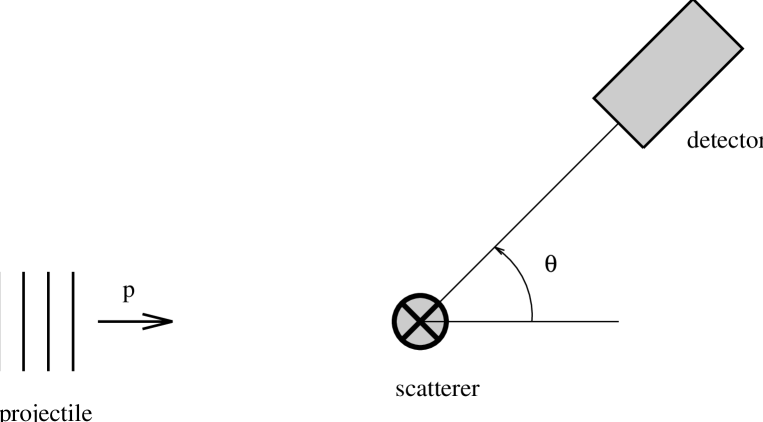
Figure 1.13: The geometry of the Aharonov-Bohm scattering experiment. The projectile comes in as a plane wave with momentum $p$ and scatters elastically from a scatterer fixed at the origin. It is assumed that the projectile never enters the region where the scatterer is located. The cross section for the scattered projectile is measured by a detector placed at the scattering angle $\theta$.

The geometry of the Aharonov-Bohm scattering experiment is depicted in figure 1.13. It involves two particles, a projectile and a scatterer fixed at the origin. The incoming external part of the total wave function is a plane wave for the projectile vanishing at the location of the scatterer. Nontrivial scattering takes place if the monodromy matrix ${\cal R}^{2}$ acting on the internal part of the wave function is nontrivial.

In the abelian discrete gauge theory discussed in section 1.3, we only encountered the abelian version, that is, the effect of a monodromy of the two particles in the internal wave function is just a phase

$${\cal R}^{2} = e^{2\pi\imath\alpha}.$$ (1.A.1)

The differential cross section for the quantum mechanical scattering experiment involving such particles has been derived by Aharonov and Bohm [4]

$$\frac{{\rm d}\sigma}{{\rm d}\theta} = \frac{\sin^{2}{(\pi\alpha})}{2\pi p\sin^{2}(\theta/2)}\;,$$ (1.A.2)

with $\theta$ the scattering angle and $p$ the momentum of the incoming plane wave of the projectile.

The particles appearing in a nonabelian discrete gauge theory, can exchange internal flux/charge quantum numbers when they encircle each other. This effect is described by nondiagonal monodromy matrices ${\cal R}^{2}$ acting on multi-component internal wave functions. The cross section measured in Aharonov-Bohm scattering experiment involving these particles is a ‘nonabelian’ generalization of the abelian one given in (1.A.2). An elegant closed formula for these nonabelian cross sections has been derived by Erik Verlinde [126]. The crucial insight was that the monodromy matrix ${\cal R}^{2}$ for two particles can always be diagonalized, since the braid group for two particles is abelian. In the monodromy eigenbasis in which the monodromy matrix ${\cal R}^{2}$ is diagonal, the nonabelian problem then reduces to the abelian one solved by Aharonov and Bohm. The solution can subsequently be cast in the basis independent form

$$\frac{{\rm d}\sigma}{{\rm d}\theta}|_{\mbox{in}\rightarrow\mbox{all}} = \frac{1}{4\pi p\sin^{2}(\theta/2)}\;\;[1-\mbox{Re}\langle\mbox{in}|{\cal R}^{2}|\mbox{in}\rangle],$$ (1.A.3)

with $|\mbox{in}\rangle$ the normalized two particle incoming internal quantum state. Note that this cross section boils down to (1.A.2) for the abelian case. We will always work in the natural two particle flux/charge eigenbasis being the tensor product of the single particle internal basis states (1.5.6). In fact, in our applications the $|\mbox{in}\rangle$ state usually is a particular two particle flux/charge eigenstate. The detector measuring the cross section (1.A.3) is a device which does not discriminate between the different internal ‘disguises’ the scattered projectile can take. Specifically, in the scattering process discussed in section 1.6.2, the Verlinde detector gives a signal, when the scattered pure doublet charge $\chi$ enters the apparatus with its charge orientation either up or down. In this sense, Verlinde’s cross section (1.A.3) is inclusive.

Inspired by this work, Lo and Preskill subsequently introduced a finer detector [92]. Their device is able to distinguish between the different internal appearances of the projectile. In the scattering process studied in section 1.6.2, for example, we can use a device, which only gives a signal if the projectile enters the device with its internal charge orientation up. The exclusive cross section measured with such a detector can be expressed as

$$\frac{{\rm d}\sigma}{{\rm d}\theta}|_{\mbox{in}\rightarrow\mbox{out}} = \frac{1}{8\pi p\sin^{2}(\theta/2)}\;\;|\langle\mbox{out}|{\cal R}^{-\theta/\pi}({\mbox{\bf 1}}-{\cal R}^{2})|\mbox{in}\rangle|^{2},$$ (1.A.4)

where $|\mbox{in}\rangle$ and $|\mbox{out}\rangle$ denote normalized two particle incoming- and outgoing internal quantum states. The outgoing state we observe depends on the detector we have installed, but since we only measure the projectile, so ‘half’ of the out state, the state $|\mbox{out}\rangle$ in (1.A.4) should always be summed over a complete basis for the internal Hilbert space of the scatterer. The new ingredient in the exclusive cross section (1.A.4) is the matrix ${\cal R}^{-\theta/\pi}$. This matrix is defined as the diagonal matrix in the monodromy eigenbasis, which acts as

$${\cal R}^{-\theta/\pi} := e^{-\imath\alpha\theta}\qquad\qquad\mbox{with $\alpha\in[0,1)$,}$$ (1.A.5)

on a monodromy eigenstate characterized by the eigenvalue $\exp(2\pi\imath\alpha)$ under ${\cal R}^{2}$. By a basis transformation, we then find the matrix elements of ${\cal R}^{-\theta/\pi}$ in our favourite two particle flux/charge eigenbasis.

A peculiar property of the exclusive cross section (1.A.4) is that it is in general multi-valued. This is just a reflection of the fact that the detector can generally change its nature, when it is parallel transported around the scatterer. An apparatus that only detects projectiles with internal charge orientation up in the scattering process studied in section 1.6.2, for example, becomes an apparatus, which only detects projectiles with charge orientation down, after a rotation over an angle of $2\pi$ around the scatterer. Verlinde’s detector, giving a signal independent of the internal ‘disguise’ of the projectile entering the device, obviously does not suffer from this multi-valuedness. As a matter of fact, extending the aforementioned sum of the $|\mbox{out}\rangle$ state in (1.A.4) over a complete basis of the internal Hilbert space for the scatterer by a sum over a complete basis of the internal Hilbert space for the projectile and subsequently using the partition of unity, yields the single valued inclusive cross section (1.A.3).

As a last remark, the cross sections for Aharonov-Bohm scattering experiments in which the projectile and the scatterer are indistinguishable particles contain an extra contribution due to conceivable exchange processes between the scatterer and the projectile [92, 129]. The incorporation of this exchange contribution amounts to diagonalizing the braid matrix ${\cal R}$ instead of the monodromy matrix ${\cal R}^{2}$.

1.B $B(3,4)$ and $P(3,4)$

In this appendix, we give the structure of the truncated braid group $B(3,4)$ and the truncated colored braid group $P(3,4)$, which enter the discussion of the nonabelian braid properties of certain three particle configurations in a $\bar{D}_{2}$ gauge theory in section 1.6.3.

According to the general definition (1.5.26)-(1.5.27), the truncated braid group $B(3,4)$ for three indistinguishable particles is generated by two elements $\tau_{1}$ and $\tau_{2}$ subject to the relations

$$\tau_{1}\tau_{2}\tau_{1} = \tau_{2}\tau_{1}\tau_{2}$$

$$\tau_{1}^{4} = \tau_{2}^{4}\;\,=\;\,e.$$

By explicit construction from these defining relations, which is a lengthy and not at all trivial job, it can be inferred that $B(3,4)$ is a group of order 96, which splits up into the following conjugacy classes

$$C_{0}^{1} = \{e\}$$ (1.B.1)

$$C_{0}^{2} = \{\tau_{1}\tau_{2}\tau_{1}\tau_{2}\tau_{1}\tau_{2}\}$$

$$C_{0}^{3} = \{\tau_{2}^{2}\tau_{1}^{2}\tau_{2}^{2}\tau_{1}^{2}\}$$

$$C_{0}^{4} = \{\tau_{2}^{2}\tau_{1}^{3}\tau_{2}^{2}\tau_{1}^{3}\}$$

$$C_{1}^{1} = \{\tau_{1}\;,\;\tau_{2}\;,\;\tau_{2}\tau_{1}\tau_{2}^{3}\;,\;\tau_{2}^{2}\tau_{1}\tau_{2}^{2}\;,\;\tau_{2}^{3}\tau_{1}\tau_{2}\;,\;\tau_{1}^{2}\tau_{2}\tau_{1}^{2}\}$$

$$C_{1}^{2} = \{\tau_{1}^{3}\tau_{2}\tau_{1}^{2}\tau_{2}\;,\;\tau_{2}^{3}\tau_{1}\tau_{2}^{2}\tau_{1}\;,\;\tau_{2}\tau_{1}^{3}\tau_{2}\tau_{1}^{2}\;,\;\tau_{2}^{2}\tau_{1}^{2}\tau_{2}^{2}\tau_{1}\;,\;\tau_{1}\tau_{2}^{3}\tau_{1}\tau_{2}^{2}\;,\;\tau_{1}^{2}\tau_{2}^{2}\tau_{1}^{2}\tau_{2}\}$$

$$C_{1}^{3} = \{\tau_{2}\tau_{1}^{3}\tau_{2}\tau_{1}^{3}\tau_{2}\;,\;\tau_{1}^{2}\tau_{2}\tau_{1}^{3}\tau_{2}^{2}\tau_{1}\;,\;\tau_{2}^{3}\tau_{1}\tau_{2}^{3}\tau_{1}^{2}\;,\;\tau_{1}\tau_{2}^{2}\tau_{1}^{3}\tau_{2}^{2}\tau_{1}\;,\;\tau_{2}\tau_{1}\tau_{2}^{3}\tau_{1}^{2}\tau_{2}^{2}\;,\;\tau_{2}\tau_{1}^{2}\tau_{2}^{3}\tau_{1}^{2}\tau_{2}\}$$

$$C_{1}^{4} = \{\tau_{2}^{2}\tau_{1}^{3}\tau_{2}^{2}\;,\;\tau_{1}^{2}\tau_{2}^{3}\tau_{1}^{2}\;,\;\tau_{2}^{3}\tau_{1}^{3}\tau_{2}\;,\;\tau_{1}^{3}\;,\;\tau_{2}\tau_{1}^{3}\tau_{2}^{3}\;,\;\tau_{2}^{3}\}$$

$$C_{2}^{1} = \{\tau_{1}\tau_{2}\;,\;\tau_{2}\tau_{1}\;,\;\tau_{1}^{2}\tau_{2}\tau_{1}^{3}\;,\;\tau_{1}^{3}\tau_{2}\tau_{1}^{2}\;,\;\tau_{2}\tau_{1}^{2}\tau_{2}^{2}\tau_{1}\;,\;\tau_{2}^{2}\tau_{1}\tau_{2}^{3}\;,\;\tau_{2}^{3}\tau_{1}\tau_{2}^{2}\;,\;\tau_{1}\tau_{2}^{2}\tau_{1}^{2}\tau_{2}\}$$

$$C_{2}^{2} = \{\tau_{1}^{2}\tau_{2}\tau_{1}^{3}\tau_{2}\tau_{1}\;,\;\tau_{1}\tau_{2}\tau_{1}^{3}\tau_{2}\tau_{1}^{2}\;,\;\tau_{2}\tau_{1}^{2}\tau_{2}^{2}\tau_{1}^{3}\;,\;\tau_{1}\tau_{2}\tau_{1}^{2}\tau_{2}^{2}\tau_{1}^{2}\;,\;$$

$$\;\tau_{2}\tau_{1}^{3}\tau_{2}^{2}\tau_{1}^{2}\;,\;\tau_{1}\tau_{2}\tau_{1}^{3}\tau_{2}^{2}\tau_{1}\;,\;\tau_{1}^{2}\tau_{2}\tau_{1}^{3}\tau_{2}^{2}\;,\;\tau_{1}^{2}\tau_{2}^{2}\tau_{1}^{3}\tau_{2}\}$$

$$C_{2}^{3} = \{\tau_{1}^{3}\tau_{2}\tau_{1}^{3}\tau_{2}^{2}\tau_{1}\;,\;\tau_{1}\tau_{2}^{2}\tau_{1}^{3}\tau_{2}\tau_{1}^{3}\;,\;\tau_{2}\tau_{1}^{3}\tau_{2}^{2}\;,\;\tau_{2}^{2}\tau_{1}^{3}\tau_{2}\;,\;\tau_{2}^{3}\tau_{1}^{3}\;,\;\tau_{1}\tau_{2}^{3}\tau_{1}^{2}\;,\;\tau_{1}^{2}\tau_{2}^{3}\tau_{1}\;,\;\tau_{1}^{3}\tau_{2}^{3}\}$$

$$C_{2}^{4} = \{\tau_{1}^{3}\tau_{2}^{3}\tau_{1}^{2}\;,\;\tau_{1}^{2}\tau_{2}^{3}\tau_{1}^{3}\;,\;\tau_{2}^{3}\tau_{1}\;,\;\tau_{1}\tau_{2}^{3}\;,\;\tau_{1}\tau_{2}\tau_{1}\tau_{2}\;,\;\tau_{1}^{3}\tau_{2}\;,\;\tau_{2}\tau_{1}^{3}\;,\;\tau_{2}\tau_{1}\tau_{2}\tau_{1}\}$$

$$C_{3}^{1} = \{\tau_{1}^{2}\;,\;\tau_{2}^{2}\;,\;\tau_{1}\tau_{2}^{2}\tau_{1}^{3}\;,\;\tau_{2}^{2}\tau_{1}^{2}\tau_{2}^{2}\;,\;\tau_{1}^{2}\tau_{2}^{2}\tau_{1}^{2}\;,\;\tau_{1}^{3}\tau_{2}^{2}\tau_{1}\}$$

$$C_{3}^{2} = \{\tau_{2}\tau_{1}^{2}\tau_{2}\;,\;\tau_{1}\tau_{2}^{2}\tau_{1}\;,\;\tau_{1}^{2}\tau_{2}^{2}\;,\;\tau_{2}^{3}\tau_{1}^{2}\tau_{2}^{3}\;,\;\tau_{1}^{3}\tau_{2}^{2}\tau_{1}^{3}\;,\;\tau_{2}^{2}\tau_{1}^{2}\}$$

$$C_{4}^{1} = \{\tau_{1}\tau_{2}\tau_{1}\;,\;\tau_{1}^{2}\tau_{2}\;,\;\tau_{2}^{2}\tau_{1}\;,\;\tau_{2}\tau_{1}^{2}\;,\;\tau_{1}\tau_{2}^{2}\;,\;\tau_{1}^{3}\tau_{2}\tau_{1}^{3}\;,\;\tau_{1}^{3}\tau_{2}\tau_{1}^{3}\tau_{2}^{2}\tau_{1}^{2}\;,\;$$

$$\;\tau_{2}\tau_{1}^{3}\tau_{2}^{2}\tau_{1}\;,\;\tau_{1}^{2}\tau_{2}^{2}\tau_{1}^{3}\;,\;\tau_{1}\tau_{2}^{2}\tau_{1}^{3}\tau_{2}\;,\;\tau_{1}^{3}\tau_{2}^{2}\tau_{1}^{2}\;,\;\tau_{1}\tau_{2}\tau_{1}^{3}\tau_{2}^{2}\}$$

$$C_{4}^{2} = \{\tau_{1}\tau_{2}\tau_{1}\tau_{2}\tau_{1}\tau_{2}\tau_{1}\tau_{2}\tau_{1}\;,\;\tau_{2}\tau_{1}^{2}\tau_{2}^{2}\;,\;\tau_{1}\tau_{2}^{2}\tau_{1}^{2}\;,\;\tau_{2}^{2}\tau_{1}^{2}\tau_{2}\;,\;\tau_{1}^{2}\tau_{2}^{2}\tau_{1}\;,\;\tau_{2}\tau_{1}^{3}\tau_{2}\;,\;$$

$$\;\tau_{2}^{3}\tau_{1}^{3}\tau_{2}^{3}\;,\;\tau_{2}^{3}\tau_{1}^{2}\;,\;\tau_{1}^{3}\tau_{2}^{2}\;,\;\tau_{2}^{2}\tau_{1}^{3}\;,\;\tau_{1}^{2}\tau_{2}^{3}\;,\;\tau_{1}\tau_{2}^{3}\tau_{1}\}.$$

We organized the conjugacy classes such that $C_{k}^{i+1}=zC_{k}^{i}$, with $z=\tau_{1}\tau_{2}\tau_{1}\tau_{2}\tau_{1}\tau_{2}$ the generator of the centre of $B(3,4)$. The character table of the truncated braid group $B(3,4)$ is displayed in table 1.4.

The truncated colored braid group $P(3,4)$, which contains the monodromy operations on a configuration of three distinguishable particles, is the subgroup of $B(3,4)$ generated by

$$\gamma_{12} = \tau_{1}^{2}$$

$$\gamma_{13} = \tau_{1}\tau_{2}^{2}\tau_{1}^{-1}=\tau_{1}\tau_{2}^{2}\tau_{1}^{3}$$ (1.B.2)

$$\gamma_{23} = \tau_{2}^{2},$$

which satisfy

$$\gamma_{12}^{2}\;=\;\gamma_{13}^{2}\;=\;\gamma_{23}^{2}\;=\;e.$$

It can be verified that $P(3,4)$ is a group of order 16 splitting up in the following 10 conjugacy classes

$$\begin{array}[]{lcl lcl}C_{0}&=&\{e\}&\qquad C_{1}&=&\{\tau_{1}\tau_{2}\tau_{1}\tau_{2}\tau_{1}\tau_{2}\}\\ C_{2}&=&\{\tau_{2}^{2}\tau_{1}^{2}\tau_{2}^{2}\tau_{1}^{2}\}&\qquad C_{3}&=&\{\tau_{2}^{2}\tau_{1}^{3}\tau_{2}^{2}\tau_{1}^{3}\}\\ C_{4}&=&\{\tau_{1}^{2}\;,\;\tau_{2}^{2}\tau_{1}^{2}\tau_{2}^{2}\}&\qquad C_{5}&=&\{\tau_{2}^{2}\;,\;\tau_{1}^{2}\tau_{2}^{2}\tau_{1}^{2}\}\\ C_{6}&=&\{\tau_{1}\tau_{2}^{2}\tau_{1}^{3}\;,\;\tau_{1}^{3}\tau_{2}^{2}\tau_{1}\}&\qquad C_{7}&=&\{\tau_{1}\tau_{2}^{2}\tau_{1}\;,\;\tau_{1}^{3}\tau_{2}^{2}\tau_{1}^{3}\}\\ C_{8}&=&\{\tau_{2}\tau_{1}^{2}\tau_{2}\;,\;\tau_{2}^{3}\tau_{1}^{2}\tau_{2}^{3}\}&\qquad C_{9}&=&\{\tau_{1}^{2}\tau_{2}^{2}\;,\;\tau_{2}^{2}\tau_{1}^{2}\}.\end{array}$$ (1.B.8)

For convenience, we expressed the elements of $P(3,4)$ in terms of the braid generators $\tau_{1}$ and $\tau_{2}$ rather than the monodromy generators $\gamma_{12}$, $\gamma_{13}$ and $\gamma_{23}$. It turns out that $P(3,4)$ is the coxeter group denoted as $16/8$ in [121]. Its centre of order four contained in the first four conjugacy classes naturally coincides with that of $B(3,4)$. The character table of this group is exhibited in table 1.5.

	${\displaystyle C_{0}^{1}}$	${\displaystyle C_{0}^{2}}$	${\displaystyle C_{0}^{3}}$	${\displaystyle C_{0}^{4}}$	${\displaystyle C_{1}^{1}}$	${\displaystyle C_{1}^{2}}$	${\displaystyle C_{1}^{3}}$	${\displaystyle C_{1}^{4}}$	${\displaystyle C_{2}^{1}}$	${\displaystyle C^{2}_{2}}$	${\displaystyle C^{3}_{2}}$	${\displaystyle C^{4}_{2}}$	${\displaystyle C_{3}^{1}}$	${\displaystyle C_{3}^{2}}$	${\displaystyle C_{4}^{1}}$	${\displaystyle C_{4}^{2}}$
${\displaystyle\Lambda_{0}}$	${\displaystyle 1}$	${\displaystyle 1}$	${\displaystyle 1}$	${\displaystyle 1}$	${\displaystyle 1}$	${\displaystyle 1}$	${\displaystyle 1}$	${\displaystyle 1}$	${\displaystyle 1}$	${\displaystyle 1}$	${\displaystyle 1}$	${\displaystyle 1}$	${\displaystyle 1}$	${\displaystyle 1}$	${\displaystyle 1}$	${\displaystyle 1}$
${\displaystyle\Lambda_{1}}$	${\displaystyle 1}$	-${\displaystyle 1}$	${\displaystyle 1}$	-${\displaystyle 1}$	${\displaystyle\imath}$	-${\displaystyle\imath}$	${\displaystyle\imath}$	-${\displaystyle\imath}$	-${\displaystyle 1}$	${\displaystyle 1}$	-${\displaystyle 1}$	${\displaystyle 1}$	-${\displaystyle 1}$	${\displaystyle 1}$	-${\displaystyle\imath}$	${\displaystyle\imath}$
${\displaystyle\Lambda_{2}}$	${\displaystyle 1}$	${\displaystyle 1}$	${\displaystyle 1}$	${\displaystyle 1}$	-${\displaystyle 1}$	-${\displaystyle 1}$	-${\displaystyle 1}$	-${\displaystyle 1}$	${\displaystyle 1}$	${\displaystyle 1}$	${\displaystyle 1}$	${\displaystyle 1}$	${\displaystyle 1}$	${\displaystyle 1}$	-${\displaystyle 1}$	-${\displaystyle 1}$
${\displaystyle\Lambda_{3}}$	${\displaystyle 1}$	-${\displaystyle 1}$	${\displaystyle 1}$	-${\displaystyle 1}$	-${\displaystyle\imath}$	${\displaystyle\imath}$	-${\displaystyle\imath}$	${\displaystyle\imath}$	-${\displaystyle 1}$	${\displaystyle 1}$	-${\displaystyle 1}$	${\displaystyle 1}$	-${\displaystyle 1}$	${\displaystyle 1}$	${\displaystyle\imath}$	-${\displaystyle\imath}$
${\displaystyle\Lambda_{4}}$	${\displaystyle 2}$	${\displaystyle 2}$	${\displaystyle 2}$	${\displaystyle 2}$	${\displaystyle 0}$	${\displaystyle 0}$	${\displaystyle 0}$	${\displaystyle 0}$	-${\displaystyle 1}$	-${\displaystyle 1}$	-${\displaystyle 1}$	-${\displaystyle 1}$	${\displaystyle 2}$	${\displaystyle 2}$	${\displaystyle 0}$	${\displaystyle 0}$
${\displaystyle\Lambda_{5}}$	${\displaystyle 2}$	-${\displaystyle 2}$	${\displaystyle 2}$	-${\displaystyle 2}$	${\displaystyle 0}$	${\displaystyle 0}$	${\displaystyle 0}$	${\displaystyle 0}$	${\displaystyle 1}$	-${\displaystyle 1}$	${\displaystyle 1}$	-${\displaystyle 1}$	-${\displaystyle 2}$	${\displaystyle 2}$	${\displaystyle 0}$	${\displaystyle 0}$
${\displaystyle\Lambda_{6}}$	${\displaystyle 2}$	${\displaystyle 2\imath}$	-${\displaystyle 2}$	-${\displaystyle 2\imath}$	${\displaystyle\eta}$	-${\displaystyle\eta^{*}}$	-${\displaystyle\eta}$	${\displaystyle\eta^{*}}$	${\displaystyle\imath}$	-${\displaystyle 1}$	-${\displaystyle\imath}$	${\displaystyle 1}$	${\displaystyle 0}$	${\displaystyle 0}$	${\displaystyle 0}$	${\displaystyle 0}$
${\displaystyle\Lambda_{7}}$	${\displaystyle 2}$	${\displaystyle 2\imath}$	-${\displaystyle 2}$	-${\displaystyle 2\imath}$	-${\displaystyle\eta}$	${\displaystyle\eta^{*}}$	${\displaystyle\eta}$	-${\displaystyle\eta^{*}}$	${\displaystyle\imath}$	-${\displaystyle 1}$	-${\displaystyle\imath}$	${\displaystyle 1}$	${\displaystyle 0}$	${\displaystyle 0}$	${\displaystyle 0}$	${\displaystyle 0}$
${\displaystyle\Lambda_{8}}$	${\displaystyle 2}$	-${\displaystyle 2\imath}$	-${\displaystyle 2}$	${\displaystyle 2\imath}$	-${\displaystyle\eta^{*}}$	${\displaystyle\eta}$	${\displaystyle\eta^{*}}$	-${\displaystyle\eta}$	-${\displaystyle\imath}$	-${\displaystyle 1}$	${\displaystyle\imath}$	${\displaystyle 1}$	${\displaystyle 0}$	${\displaystyle 0}$	${\displaystyle 0}$	${\displaystyle 0}$
${\displaystyle\Lambda_{9}}$	${\displaystyle 2}$	-${\displaystyle 2\imath}$	-${\displaystyle 2}$	${\displaystyle 2\imath}$	${\displaystyle\eta^{*}}$	-${\displaystyle\eta}$	-${\displaystyle\eta^{*}}$	${\displaystyle\eta}$	-${\displaystyle\imath}$	-${\displaystyle 1}$	${\displaystyle\imath}$	${\displaystyle 1}$	${\displaystyle 0}$	${\displaystyle 0}$	${\displaystyle 0}$	${\displaystyle 0}$
${\displaystyle\Lambda_{10}}$	${\displaystyle 3}$	${\displaystyle 3}$	${\displaystyle 3}$	${\displaystyle 3}$	${\displaystyle 1}$	${\displaystyle 1}$	${\displaystyle 1}$	${\displaystyle 1}$	${\displaystyle 0}$	${\displaystyle 0}$	${\displaystyle 0}$	${\displaystyle 0}$	-${\displaystyle 1}$	-${\displaystyle 1}$	-${\displaystyle 1}$	-${\displaystyle 1}$
${\displaystyle\Lambda_{11}}$	${\displaystyle 3}$	-${\displaystyle 3}$	${\displaystyle 3}$	-${\displaystyle 3}$	${\displaystyle\imath}$	-${\displaystyle\imath}$	${\displaystyle\imath}$	-${\displaystyle\imath}$	${\displaystyle 0}$	${\displaystyle 0}$	${\displaystyle 0}$	${\displaystyle 0}$	${\displaystyle 1}$	-${\displaystyle 1}$	${\displaystyle\imath}$	-${\displaystyle\imath}$
${\displaystyle\Lambda_{12}}$	${\displaystyle 3}$	${\displaystyle 3}$	${\displaystyle 3}$	${\displaystyle 3}$	-${\displaystyle 1}$	-${\displaystyle 1}$	-${\displaystyle 1}$	-${\displaystyle 1}$	${\displaystyle 0}$	${\displaystyle 0}$	${\displaystyle 0}$	${\displaystyle 0}$	-${\displaystyle 1}$	-${\displaystyle 1}$	${\displaystyle 1}$	${\displaystyle 1}$
${\displaystyle\Lambda_{13}}$	${\displaystyle 3}$	-${\displaystyle 3}$	${\displaystyle 3}$	-${\displaystyle 3}$	-${\displaystyle\imath}$	${\displaystyle\imath}$	-${\displaystyle\imath}$	${\displaystyle\imath}$	${\displaystyle 0}$	${\displaystyle 0}$	${\displaystyle 0}$	${\displaystyle 0}$	${\displaystyle 1}$	-${\displaystyle 1}$	-${\displaystyle\imath}$	${\displaystyle\imath}$
${\displaystyle\Lambda_{14}}$	${\displaystyle 4}$	${\displaystyle 4}$	-${\displaystyle 4}$	-${\displaystyle 4}$	${\displaystyle 0}$	${\displaystyle 0}$	${\displaystyle 0}$	${\displaystyle 0}$	${\displaystyle 1}$	${\displaystyle 1}$	-${\displaystyle 1}$	-${\displaystyle 1}$	${\displaystyle 0}$	${\displaystyle 0}$	${\displaystyle 0}$	${\displaystyle 0}$
${\displaystyle\Lambda_{15}}$	${\displaystyle 4}$	-${\displaystyle 4}$	-${\displaystyle 4}$	${\displaystyle 4}$	${\displaystyle 0}$	${\displaystyle 0}$	${\displaystyle 0}$	${\displaystyle 0}$	-${\displaystyle 1}$	${\displaystyle 1}$	${\displaystyle 1}$	-${\displaystyle 1}$	${\displaystyle 0}$	${\displaystyle 0}$	${\displaystyle 0}$	${\displaystyle 0}$

Table 1.4: Character table of the truncated braid group $B(3,4)$. We used $\eta:=\imath+1$.

$P(3,4)$		$C_{0}$	$C_{1}$	$C_{1}$	$C_{3}$	$C_{4}$	$C_{5}$	$C_{6}$	$C_{7}$	$C_{8}$	$C_{9}$
$\Omega_{0}$		$1$	$1$	$1$	$1$	$1$	$1$	$1$	$1$	$1$	$1$
$\Omega_{1}$		$1$	$1$	$1$	$1$	$-1$	$-1$	$1$	$-1$	$-1$	$1$
$\Omega_{2}$		$1$	$1$	$1$	$1$	$-1$	$1$	$-1$	$1$	$-1$	$-1$
$\Omega_{3}$		$1$	$1$	$1$	$1$	$1$	$-1$	$-1$	$-1$	$1$	$-1$
$\Omega_{4}$		$1$	$-1$	$1$	$-1$	$-1$	$1$	$1$	$-1$	$1$	$-1$
$\Omega_{5}$		$1$	$-1$	$1$	$-1$	$1$	$-1$	$1$	$1$	$-1$	$-1$
$\Omega_{6}$		$1$	$-1$	$1$	$-1$	$1$	$1$	$-1$	$-1$	$-1$	$1$
$\Omega_{7}$		$1$	$-1$	$1$	$-1$	$-1$	$-1$	$-1$	$1$	$1$	$1$
$\Omega_{8}$		$2$	$2\imath$	$-2$	$-2\imath$	$0$	$0$	$0$	$0$	$0$	$0$
$\Omega_{9}$		$2$	$-2\imath$	$-2$	$2\imath$	$0$	$0$	$0$	$0$	$0$	$0$

Table 1.5: Character table of the truncated colored braid group $P(3,4)$.

Chapter 2 Abelian Chern-Simons theories

2.1 Introduction

A characteristic feature of three dimensional space time is the possibility to endow a gauge theory with a so-called Chern-Simons term [45, 113]. It is well-known that the incorporation of such a term renders a gauge theory topological. That is, the gauge fields acquire a topological mass, whereas the charges coupled to the gauge fields now induce magnetic fluxes and as a result exhibit nontrivial braid statistics (e.g. [63, 136]). This is roughly speaking the effect of adding a Chern-Simons term to an unbroken continuous gauge theory. Here, we will study the implications of adding a Chern-Simons term to the spontaneously broken planar gauge theories discussed in the previous chapter [19, 20, 21]. Hence, the models under consideration are governed by an action of the form

$$S = S_{\mbox{\scriptsize YMH}}+S_{\mbox{\scriptsize matter}}+S_{\mbox{\scriptsize CS}}\,,$$ (2.1.1)

where the Yang-Mills Higgs action $S_{\rm{\mbox{\scriptsize YMH}}}$ again gives rise to the spontaneous breakdown of the continuous compact gauge group $G$ to a finite subgroup ${H}$ and $S_{\mbox{\scriptsize matter}}$ describes a conserved matter current minimally coupled to the gauge fields. Finally, $S_{\rm{CS}}$ denotes the Chern-Simons action for the gauge fields. For convenience, we restrict ourselves to abelian broken Chern-Simons gauge theories (2.1.1) and return to the nonabelian case in chapter 3. To be specific, in the present chapter we focus on symmetry breaking schemes

$${G}\;\simeq\;U(1)^{k} \longrightarrow {H}\,,$$ (2.1.2)

with $U(1)^{k}$ the direct product of $k$ compact $U(1)$ gauge groups and the finite subgroup $H$ a direct product of $k$ cyclic groups ${\mbox{\bf Z}}_{N^{(i)}}$ of order $N^{(i)}$

$${H} \simeq {\mbox{\bf Z}}_{N^{(1)}}\times{\mbox{\bf Z}}_{N^{(2)}}\times\cdots\times{\mbox{\bf Z}}_{N^{(k)}}\,.$$ (2.1.3)

The Chern-Simons terms for the gauge group $U(1)^{k}$ are known to fall into two types, see for example [128] and references therein. On the one hand, there are terms that describe self-couplings of the various $U(1)$ gauge fields. These will be called Chern-Simons terms of type I for convenience. On the other hand, there are terms (type II) that establish couplings between two different $U(1)$ gauge fields. To be concrete, the most general Chern-Simons action for the gauge group $U(1)\times U(1)$, for instance, is of the form

$$S_{\mbox{\scriptsize CS}} = \int d\,^{3}x\;(\,\frac{\mu^{(12)}}{2}\epsilon^{\kappa\sigma\rho}A^{(1)}_{\kappa}\partial_{\sigma}A^{(2)}_{\rho}\>+\>\sum_{i=1}^{2}\frac{\mu^{(i)}}{2}\epsilon^{\kappa\sigma\rho}A^{(i)}_{\kappa}\partial_{\sigma}A^{(i)}_{\rho}\,),$$ (2.1.4)

with $A_{\kappa}^{(1)}$ and $A_{\kappa}^{(2)}$ the two $U(1)$ gauge fields. The parameters $\mu^{(1)}$, $\mu^{(2)}$ denote the topological masses characterizing the two Chern-Simons terms of type I and $\mu^{(12)}$ the topological mass characterizing the Chern-Simons term of type II. In the unbroken phase, these Chern-Simons terms assign magnetic fluxes to the quantized matter charges $q^{(1)}$ and $q^{(2)}$ coupled to the two compact $U(1)$ gauge fields. Specifically, the type I Chern-Simons term for the gauge field $A_{\kappa}^{(i)}$ attaches a magnetic flux $\phi^{(i)}=-q^{(i)}/\mu^{(i)}$ to a matter charge $q^{(i)}=n^{(i)}e^{(i)}$ with $n^{(i)}\in{\mbox{\bf Z}}$ and $e^{(i)}$ the fundamental charge for $A_{\kappa}^{(i)}$. As a consequence, there are nontrivial topological interactions among these charges. When a charge $q^{(i)}$ encircles a remote charge $q^{(i)^{\prime}}$ in a counterclockwise fashion, the wave function acquires the Aharonov-Bohm phase $\exp(-\imath q^{(i)}q^{(i)^{\prime}}/\mu^{(i)})$ [63]. The Chern-Simons term of type II, in turn, attaches fluxes which belong to one $U(1)$ gauge group to the matter charges of the other. That is, a charge $q^{(1)}$ induces a flux $\phi^{(2)}=-2q^{(1)}/\mu^{(12)}$ and a charge $q^{(2)}$ induces a flux $\phi^{(1)}=-2q^{(2)}/\mu^{(12)}$. Hence, the type II Chern-Simons term gives rise to topological interactions among matter charges of the two different $U(1)$ gauge groups. A counterclockwise monodromy of a charge $q^{(1)}$ and a charge $q^{(2)}$, for example, yields the Aharonov-Bohm phase $\exp(-2\imath q^{(1)}q^{(2)}/\mu^{(12)})$, e.g. [56, 65, 80, 128, 132].

The presence of a Chern-Simons term for the continuous gauge group $U(1)^{k}$ naturally has a bearing on the topological interactions in the broken phase. As we will argue, it gives rise to nontrivial Aharonov-Bohm phases among the vortices labeled by the elements of the residual gauge group (2.1.3). To be specific, the $k$ different vortex species carry quantized flux $\phi^{(i)}=\frac{2\pi a^{(i)}}{N^{(i)}e^{(i)}}$ with $a^{(i)}\in{\mbox{\bf Z}}$ and $N^{(i)}$ the order of the $i^{\rm th}$ cyclic group of the product group (2.1.3). A type I Chern-Simons term for the gauge field $A_{\kappa}^{(i)}$ then implies the Aharonov-Bohm phase $\exp(\imath\mu^{(i)}\phi^{(i)}\phi^{(i)^{\prime}})$ for a counterclockwise monodromy of a vortex $\phi^{(i)}$ and a vortex $\phi^{(i)^{\prime}}$. A Chern-Simons term of type II coupling the gauge fields $A_{\kappa}^{(i)}$ and $A_{\kappa}^{(j)}$, in turn, gives rise to the Aharonov-Bohm phase $\exp(\imath\mu^{(ij)}\phi^{(i)}\phi^{(j)})$ for the process in which a vortex $\phi^{(i)}$ circumnavigates a vortex $\phi^{(j)}$ in a counterclockwise fashion. In fact, these additional Aharonov-Bohm phases among the vortices form the only distinction with the abelian discrete $H$ gauge theory describing the long distance physics in the absence of a Chern-Simons action for the broken gauge group $U(1)^{k}$. That is, the Higgs mechanism removes the fluxes attached the matter charges $q^{(i)}$ in the unbroken Chern-Simons phase. Hence, contrary to the unbroken Chern-Simons phase, there are no Aharonov-Bohm interactions among the matter charges in the Chern-Simons Higgs phase [19, 20, 21]. The canonical Aharonov-Bohm interactions $\exp(\imath q^{(i)}\phi^{(i)})$ between the matter charges $q^{(i)}$ and the magnetic vortices $\phi^{(i)}$ persist though.

The organization of this chapter is as follows. In section 2.2, we very briefly recall that the Chern-Simons actions for a compact gauge group $G$ are classified by the cohomology group $H^{4}(BG,{\mbox{\bf Z}})$ of the classifying space $BG$ [47]. For finite groups $H$, this classification boils down to the cohomology group $H^{3}(H,U(1))$ of the group $H$ itself. In other words, the different Chern-Simons theories for a finite gauge group $H$ correspond to the independent 3-cocycles $\omega\in H^{3}(H,U(1))$, which describe additional Aharonov-Bohm interactions among the fluxes labeled by the elements of $H$. We then note that the inclusion $H\subset G$ induces a natural homomorphism $H^{4}(BG,{\mbox{\bf Z}})\to H^{3}(H,U(1))$. This homomorphism determines the discrete $H$ Chern-Simons theory $\omega\in H^{3}(H,U(1))$ describing the long distance physics of the Chern-Simons theory $S_{\mbox{\scriptsize CS}}\in H^{4}(BG,{\mbox{\bf Z}})$ in which the continuous gauge group $G$ is broken to the finite subgroup $H$. Section 2.3 subsequently contains a short introduction to the cohomology groups $H^{n}(H,U(1))$ of finite abelian groups $H$. In particular, we give the explicit realization of the complete set of independent 3-cocycles $\omega\in H^{3}(H,U(1))$ for the abelian groups (2.1.3). It turns out that these split up into three different types, namely 3-cocycles (type I) which give rise to Aharonov-Bohm interactions among fluxes of the same cyclic gauge group in the direct product (2.1.3), those (type II) that describe interactions between fluxes corresponding to two different cyclic gauge groups and finally 3-cocycles (type III) that lead to additional Aharonov-Bohm interactions between fluxes associated to three different cyclic gauge groups. In section 2.4, we turn to the classification of Chern-Simons actions for the compact gauge group $U(1)^{k}$ and establish that the homomorphism $H^{4}(B(U(1)^{k}),{\mbox{\bf Z}})\to H^{3}(H,U(1))$ induced by the spontaneous symmetry breakdown (2.1.2) is not onto. That is, the only Chern-Simons theories with finite abelian gauge group (2.1.3) that may arise from a spontaneously broken $U(1)^{k}$ Chern-Simons theory are those corresponding to a 3-cocycle of type I and/or type II, while 3-cocycles of type III do not occur. Further, the introduction of a 3-cocycle $\omega\in H^{3}(H,U(1))$ in an abelian discrete $H$ gauge theory leads to a natural deformation of the related quantum double $D(H)$ into the quasi-quantum double $D^{\omega}(H)$. This deformation is discussed in section 2.5.

In the next sections, these general considerations are illustrated by some representative examples. Specifically, section 2.6 contains an analysis of the abelian Chern-Simons Higgs model in which the compact gauge group $G\simeq U(1)$ is broken down to the cyclic subgroup $H\simeq{\mbox{\bf Z}}_{N}$. We briefly review the unbroken phase of this model and recall that a consistent implementation of Dirac monopoles requires the topological mass to be quantized as $\mu=\frac{pe^{2}}{\pi}$ with $p\in{\mbox{\bf Z}}$ [64, 103]. This is in accordance with the fact that the different Chern-Simons actions for a compact gauge group $U(1)$ are classified by the integers: $H^{4}(BU(1),{\mbox{\bf Z}})\simeq{\mbox{\bf Z}}$. We then turn to the broken phase of the model and establish that the long distance physics is indeed described by a ${\mbox{\bf Z}}_{N}$ Chern-Simons theory with 3-cocycle $\omega\in H^{3}({\mbox{\bf Z}}_{N},U(1))\simeq{\mbox{\bf Z}}_{N}$ fixed by the natural homomorphism $H^{4}(BU(1),{\mbox{\bf Z}})\to H^{3}({\mbox{\bf Z}}_{N},U(1))$. That is, the integral Chern-Simons parameter $p$ becomes periodic in the broken phase with period $N$. Section 2.7 contains a similar treatment of a Chern-Simons theory of type II with gauge group $G\simeq U(1)\times U(1)$ spontaneously broken down to $H\simeq{\mbox{\bf Z}}_{N^{(1)}}\times{\mbox{\bf Z}}_{N^{(2)}}$. The long distance physics of this model is described by a ${\mbox{\bf Z}}_{N^{(1)}}\times{\mbox{\bf Z}}_{N^{(2)}}$ Chern-Simons theory defined by a 3-cocycle of type II. The abelian discrete $H$ Chern-Simons theories which do not occur in spontaneously broken $U(1)^{k}$ Chern-Simons theories are actually the most interesting. These are the theories defined by the aforementioned 3-cocycles of type III. The simplest example of such a theory, namely that with gauge group $H\simeq{\mbox{\bf Z}}_{2}\times{\mbox{\bf Z}}_{2}\times{\mbox{\bf Z}}_{2}$, is discussed in section 2.8. We will show that the introduction of the corresponding 3-cocycle of type III renders this theory nonabelian. In fact, this theory turns out to be dual to an ordinary $D_{4}$ gauge theory with $D_{4}$ the nonabelian dihedral group of order $8$.

In section 2.9, we briefly evaluate the Dijkgraaf-Witten invariant for some lens spaces using the three different types of 3-cocycles for various finite abelian groups $H$. Finally, in an appendix we have collected some results in the theory of cohomology which will be used in this chapter. In particular, it contains a derivation of the cohomology group $H^{3}(H,U(1))$ of an arbitrary abelian finite group (2.1.3).

As a last remark, the treatment of the examples in sections 2.6, 2.7 and 2.8 is more or less self contained. The reader could well start with section 2.6 and occasionally go back to earlier sections to fill in some details.

2.2 Group cohomology and symmetry breaking

As has been argued by Dijkgraaf and Witten [47], the Chern-Simons actions $S_{\mbox{\scriptsize CS}}$ for a compact gauge group $G$ are in one-to-one correspondence with the elements of the cohomology group $H^{4}(B{G},{\mbox{\bf Z}})$ of the classifying space $B{G}$ with integer coefficients Z. (Let $EG$ be a contractible space characterized by a free action of $G$. The classifying space $BG$ is then given by dividing out the action of $G$ on $EG$, that is, $BG=EG/G$. See for instance [53]). In particular, this classification includes the case of finite gauge groups $H$. The isomorphism [95]

$$H^{n}(B{H},{\mbox{\bf Z}}) \simeq H^{n}({H},{\mbox{\bf Z}}),$$ (2.2.1)

which only holds for finite groups ${H}$, shows that the cohomology of the classifying space $BH$ is the same as that of the group $H$ itself. In addition, we have the isomorphism

$$H^{n}(H,{\mbox{\bf Z}}) \simeq H^{n-1}({H},U(1))\qquad\forall\,n>1.$$ (2.2.2)

A derivation of this result, using the universal coefficients theorem, is contained in appendix 2.A. Especially, we now arrive at the identification

$$H^{4}({BH},{\mbox{\bf Z}}) \simeq H^{3}({H},U(1)).$$ (2.2.3)

This expresses the fact that the different Chern-Simons theories for a finite gauge group $H$ are defined by the elements $\omega\in H^{3}({H},U(1))$, i.e. algebraic 3-cocycles $\omega$ taking values in $U(1)$. These 3-cocycles can then be interpreted as $\omega=\exp(\imath S_{\mbox{\scriptsize CS}})$, where $S_{\mbox{\scriptsize CS}}$ denotes a Chern-Simons action for the finite gauge group $H$ [47]. With abuse of language, we will usually call $\omega$ itself a Chern-Simons action for $H$.

Let $K$ be a subgroup of a compact group $G$. The inclusion $K\subset G$ induces a natural homomorphism

$$H^{4}(B{G},{\mbox{\bf Z}}) \longrightarrow H^{4}(BK,{\mbox{\bf Z}})\,,$$ (2.2.4)

called the restriction (e.g. [34, 41]). This homomorphism determines the fate of a given Chern-Simons action $S_{\mbox{\scriptsize CS}}\in H^{4}(B{G},{\mbox{\bf Z}})$ when the gauge group $G$ is spontaneously broken down to $K$. That is, the mapping (2.2.4) fixes the Chern-Simons action $\in H^{4}(BK,{\mbox{\bf Z}})$ for the residual gauge group $K$ to which $S_{\mbox{\scriptsize CS}}$ reduces in the broken phase. In the following, we will only be concerned with Chern-Simons theories in which a continuous (compact) gauge group $G$ is broken down to a finite subgroup $H$. The long distance physics of such a model is described by a discrete $H$ Chern-Simons theory with 3-cocycle $\omega\in H^{3}({H},U(1))$ determined by the original Chern-Simons action $S_{\mbox{\scriptsize CS}}$ for the broken gauge group $G$. The 3-cocycle $\omega$ now governs the additional Aharonov-Bohm phases among the magnetic fluxes $h\in H$ implied by the Chern-Simons action $S_{\mbox{\scriptsize CS}}$. This is roughly speaking the physical background to the natural homomorphism

$$H^{4}(B{G},{\mbox{\bf Z}}) \longrightarrow H^{3}({H},U(1))\,,$$ (2.2.5)

which is the composition of the restriction $H^{4}(B{G},{\mbox{\bf Z}})\to H^{4}(BH,{\mbox{\bf Z}})$ induced by the inclusion $H\subset G$, and the isomorphism (2.2.3).

The restrictions (2.2.4) and (2.2.5) for continuous subgroups $K\subset G$ and finite subgroups $H\subset G$, respectively, are not necessarily onto. Hence, it is not guaranteed that all Chern-Simons theories with gauge group $K$ (or $H$) can be obtained from spontaneously broken Chern-Simons theories with gauge group $G$. Particularly, in the following sections we will see that the natural homomorphism $H^{4}(B(U(1)^{k}),{\mbox{\bf Z}})\to H^{3}(H,U(1))$ induced by the symmetry breaking (2.1.2) is not onto.

2.3 Cohomology of finite abelian groups

Here, we give a brief introduction to the cohomology groups $H^{n}({H},U(1))$ of a finite abelian group $H$. The discussion is organized as follows. In section 2.3.1, we begin by recalling the basic definitions and subsequently focus on the cocycle structure occurring in an abelian discrete $H$ Chern Simons theory. Finally, the explicit realization of all independent 3-cocycles $\omega\in H^{3}({H},U(1))$ for an arbitrary abelian group ${H}$ is given in section 2.3.2.

2.3.1 $H^{n}(H,U(1))$

In the (multiplicative) algebraic description of the cohomology groups $H^{n}(H,U(1))$, the $n$-cochains are represented as $U(1)$ valued functions

$$c:\;\underbrace{{H}\times\cdots\times{H}}_{n\;\mbox{\scriptsize times}} \longrightarrow U(1).$$ (2.3.1)

The set of all $n$-cochains forms the abelian group $C^{n}({H},U(1)):=C^{n}$ with pointwise multiplication

$$(c\cdot d)\,(A_{1},\ldots,A_{n}) = c\,(A_{1},\ldots,A_{n})\;d\,(A_{1},\ldots,A_{n}),$$

where the capitals $A_{j}$ (with $1\leq j\leq n$) denote elements of the finite group ${H}$ and $c,d\in C^{n}$. The coboundary operator $\delta$ then establishes a mapping

$$\delta:\;C^{n} \longrightarrow C^{n+1}$$

$$c \longmapsto \delta c,$$

given by

$$\delta c\,(A_{1},\ldots,A_{n+1}) = c\,(A_{2},\ldots,A_{n+1})\;c\,(A_{1},\ldots,A_{n})^{(-1)^{n+1}}$$

$$\qquad\qquad\times\prod_{i=1}^{n}c\,(A_{1},\dots,A_{i}\cdot A_{i+1},\ldots,A_{n+1})^{(-1)^{i}},$$

which acts as a derivation $\delta(c\cdot d)=\delta c\cdot\delta d$. It can be checked explicitly that $\delta$ is indeed nilpotent $\delta^{2}=1$. The coboundary operator $\delta$ naturally defines two subgroups $Z^{n}$ and $B^{n}$ of $C^{n}$. Specifically, the subgroup $Z^{n}\subset C^{n}$ consists of $n$-cocycles being the $n$-cochains $c$ in the kernel of $\delta$

$$\delta c = 1\qquad\forall\,\,c\in Z^{n},$$ (2.3.3)

whereas the subgroup $B^{n}\subset Z^{n}\subset C^{n}$ contains the $n$-coboundaries or exact $n$-cocycles

$$c = \delta b\qquad\forall\,\,c\in B^{n}.$$ (2.3.4)

with $b$ some cochain $\in C^{n-1}$. The cohomology group $H^{n}({H},U(1))$ is now defined as

$$H^{n}({H},U(1)) := Z^{n}/B^{n}.$$ (2.3.5)

In other words, the elements of $H^{n}({H},U(1))$ correspond to the $n$-cocycles (2.3.3) with equivalence relation $c\sim c\delta b$.

The so-called slant product $i_{A}$ with $A\in H$ is a mapping in the opposite direction to the coboundary operator (see for instance [120] and also appendix 3.A of chapter 3)

$$i_{A}:\;C^{n} \longrightarrow C^{n-1}$$

$$c \longmapsto i_{A}c,$$

defined as

$$i_{A}c\,(A_{1},\ldots,A_{n-1}) := c\,(A,A_{1},\ldots,A_{n-1})^{(-1)^{n-1}}$$

$$\qquad\times\prod_{i=1}^{n-1}c\,(A_{1},\ldots,A_{i},A,A_{i+1},\ldots,A_{n-1})^{(-1)^{n-1+i}}.$$

It can be shown that the slant product satisfies the following relation

$$\delta(i_{A}c) = i_{A}\,\delta c.$$ (2.3.7)

for all $n$-cochains $c$. Notably, if $c$ is a $n$-cocycle, we immediately infer from (2.3.7) that $i_{A}c$ becomes a $(n-1)$-cocycle: $\delta(i_{A}c)=i_{A}\,\delta c=1$. Hence, the slant product establishes an homomorphism

$$i_{A}:H^{n}({H},U(1)) \longrightarrow H^{n-1}({H},U(1)),$$ (2.3.8)

for each $A\in H$.

Let us finally turn to the cocycle structure appearing in an abelian discrete $H$ gauge theory with Chern-Simons action $\omega\in H^{3}({H},U(1))$. First of all, as indicated by (2.3.1) and (2.3.3), the 3-cocycle $\omega$ satisfies the relation

$$\omega(A,B,C)\;\omega(A,B\cdot C,D)\;\omega(B,C,D) = \omega(A\cdot B,C,D)\;\omega(A,B,C\cdot D),\qquad$$ (2.3.9)

for all $A,B,C\in H$. To continue, the slant product (2.3.1) as applied to $\omega$ gives rise to a set of 2-cocycles $c_{A}\in H^{2}({H},U(1))$

$$c_{A}(B,C)\;:=\;i_{A}\omega(B,C)\;=\;\frac{\omega(A,B,C)\;\omega(B,C,A)}{\omega(B,A,C)},$$ (2.3.10)

which are labeled by the different elements $A$ of $H$. As will become clear in section 2.5, these 2-cocycles enter the definition of the projective dyon charge representations associated to the magnetic fluxes in this abelian discrete $H$ Chern-Simons gauge theory. To be specific, the different charges we can assign to the abelian magnetic flux $A\in H$ to form dyons are labeled by the inequivalent unitary irreducible projective representations $\alpha$ of $H$ defined as

$${\alpha}(B)\,\cdot\,{\alpha}(C) = c_{A}(B,C)\;{\alpha}(B\cdot C).$$ (2.3.11)

Here, the 2-cocycle relation satisfied by $c_{A}$

$$c_{A}(B,C)\;c_{A}(B\cdot C,D) = c_{A}(B,C\cdot D)\;c_{A}(C,D),$$ (2.3.12)

implies that the representations $\alpha$ are associative. To conclude, as follows from (2.3.1) and (2.3.3), the 1-cocycles obey the relation $c\,(B)\;c\,(C)=c\,(B\cdot C)$. In other words, the different 1-cocycles being the elements of the cohomology group $H^{1}({H},U(1))$ correspond to the inequivalent ordinary UIR’s of the group ${H}$. These label the conceivable free charges in a Chern-Simons theory with finite abelian gauge group $H$.

2.3.2 Chern-Simons actions for finite abelian groups

In this section, we present the explicit realization of the different 3-cocycles (2.3.9) for the finite abelian groups (2.1.3) and subsequently evaluate the 2-cocycles obtained from these 3-cocycles by means of the slant product (2.3.10).

For convenience, we start with the abelian groups of the particular form ${H}\simeq{\mbox{\bf Z}}_{N}^{k}$, that is, $H$ is the direct product of $k$ cyclic groups of the same order $N$. An abstract group cohomological derivation (contained in appendix 2.A) reveals the following content of the relevant cohomology groups

$$H^{1}({\mbox{\bf Z}}_{N}^{k},U(1)) \simeq {\mbox{\bf Z}}_{N}^{k}$$ (2.3.13)

$$H^{2}({\mbox{\bf Z}}_{N}^{k},U(1)) \simeq {\mbox{\bf Z}}_{N}^{\frac{1}{2}k(k-1)}$$ (2.3.14)

$$H^{3}({\mbox{\bf Z}}_{N}^{k},U(1)) \simeq {\mbox{\bf Z}}_{N}^{k+\frac{1}{2}k(k-1)+\frac{1}{3!}k(k-1)(k-2)}.$$ (2.3.15)

As we have seen in the previous section, the first result labels the inequivalent UIR’s of ${\mbox{\bf Z}}_{N}^{k}$, the second labels the different 2-cocycles entering the projective representations of ${\mbox{\bf Z}}_{N}^{k}$, whereas the last result gives the number of different 3-cocycles or Chern-Simons actions for ${\mbox{\bf Z}}_{N}^{k}$. The derivation of the isomorphism (2.3.15) in appendix 2.A pointed out that there are, in fact, three dissimilar types of 3-cocycles. The explicit realization of these 3-cocycles involves some notational conventions, which we establish first. Let $A,B$ and $C$ denote elements of ${\mbox{\bf Z}}_{N}^{k}$, i.e.

$$A := (a^{(1)},a^{(2)},\ldots,a^{(k)})\qquad\mbox{with $a^{(i)}\in{\mbox{\bf Z}}_{N}$ for $i=1,\ldots,k$}\,,$$ (2.3.16)

and similar decompositions for $B$ and $C$. We adopt the additive presentation for the abelian group ${\mbox{\bf Z}}_{N}^{k}$, that is, the elements $a^{(i)}$ of ${\mbox{\bf Z}}_{N}$ take values in the range $0,\ldots,N-1$, and group multiplication is defined as

$$A\cdot B\;=\;[A+B]\;:=\;([a^{(1)}+b^{(1)}],\ldots,[a^{(k)}+b^{(k)}]).$$ (2.3.17)

Here, the rectangular brackets again denote modulo $N$ calculus, such that the sum always lies in the range $0,\ldots,N-1$. With these conventions, the three types of 3-cocycles for the direct product group ${\mbox{\bf Z}}_{N}^{k}$ take the following form

$$\halign to=0.0pt{\hskip\@centering$\displaystyle{#}$\@eqnsel&\global\@eqcnt\@ne\hskip\tw@\arraycolsep\hfil${#}$\hfil&\global\@eqcnt\tw@\hskip\tw@\arraycolsep$\displaystyle{#}$\hfil&\global\@eqcnt\thr@@\hskip\tw@\arraycolsep\hfil\hbox{#}&\global\@eqcnt 4 \hbox\bgroup\hss#\egroup\cr 0.0pt plus 1000.0pt$\displaystyle{\omega_{\rm I}^{(i)}(A,B,C) \!\!\! &10.0pt\hfil${=&10.0pt$\displaystyle{\!\!\! \exp\left( \frac{2 \pi\imath p^{(i)}_{\mbox{\scriptsize I}}}{N^{2}} a^{(i)}(b^{(i)} +c^{(i)} -[b^{(i)}+c^{(i)}]) \right) &10.0pt\hfil\hbox{$\!\!1\leq i\leq k$ \, \\ \omega_{\mbox{\scriptsize II}}^{(ij)}(A,B,C) \!\!\!&{\hss=}&\!\!\!\exp\left(\frac{2\pi\imath p^{(ij)}_{\mbox{\scriptsize II}}}{N^{2}}a^{(i)}(b^{(j)}+c^{(j)}-[b^{(j)}+c^{(j)}])\right)&$\!\! 1 \leq i < j \leq k$\,\\\omega_{\mbox{\scriptsize III}}^{(ijl)}(A,B,C)\!\!\!&=&\!\!\!\exp\left(\frac{2\pi\imath p^{(ijl)}_{\mbox{\scriptsize III}}}{N}a^{(i)}b^{(j)}c^{(l)}\right)&$\!\! 1 \leq i < j < l \leq k$,(2.3.18)\cr}}}}}$$

where the integral parameters $p_{\rm I}^{(i)}$, $p_{\mbox{\scriptsize II}}^{(ij)}$ and $p^{(ijl)}_{\mbox{\scriptsize III}}$ label the different elements of the cohomology group $H^{3}({\mbox{\bf Z}}_{N}^{k},U(1))$. In accordance with (2.3.15), the 3-cocycles are periodic functions of these parameters with period $N$. For the 3-cocycles of type III this periodicity is obvious, while for the 3-cocycles of type I and II it is immediate after the observation that the factors $(b^{(i)}+c^{(i)}-[b^{(i)}+c^{(i)}])$, with $1\leq i\leq k$, either vanish or equal $N$. Moreover, it is also readily checked that these 3-cocycles indeed satisfy the relation (2.3.9).

Let us proceed with a closer examination of these three types of 3-cocycles. The $k$ different 3-cocycles of type I describe self-couplings, that is, couplings between the magnetic fluxes ($a^{(i)}$,$b^{(i)}$ and $c^{(i)}$) associated to the same gauge group ${\mbox{\bf Z}}_{N}$ in the direct product ${\mbox{\bf Z}}_{N}^{k}$. In this counting procedure, it is, of course, understood that every 3-cocycle actually stands for a set of $N-1$ nontrivial 3-cocycles labeled by the periodic parameter $p_{\mbox{\scriptsize I}}^{(i)}$. The 3-cocycles of type II, in turn, establish pairwise couplings between the magnetic fluxes corresponding to different gauge groups ${\mbox{\bf Z}}_{N}$ in the direct product ${\mbox{\bf Z}}_{N}^{k}$. Note that the 3-cocycles $\omega_{\mbox{\scriptsize II}}^{(ij)}$ and $\omega_{\mbox{\scriptsize II}}^{(ji)}$ are equivalent, since they differ by a 3-coboundary (2.3.4). In other words, there are only $\frac{1}{2}k(k-1)$ distinct 3-cocycles of type II. A similar argument holds for the 3-cocycles of type III. A permutation of the labels $i$, $j$ and $k$ in these 3-cocycles yields an equivalent 3-cocycle. Hence, we end up with $\frac{1}{3!}k(k-1)(k-2)$ different 3-cocycles of type III, which realize couplings between the fluxes associated to three distinct ${\mbox{\bf Z}}_{N}$ gauge groups.

We are now well prepared to discuss the 3-cocycle structure for general abelian groups $H$ being direct products (2.1.3) of cyclic groups possibly of different order. Let us assume that ${H}$ consists of $k$ cyclic factors. The abstract analysis in appendix 2.A shows that depending on the divisibility of the orders of the different cyclic factors, there are again $k$ distinct 3-cocycles of type I, $\frac{1}{2}k(k-1)$ different 3-cocycles of type II and $\frac{1}{3!}k(k-1)(k-2)$ different 3-cocycles of type III. It is easily verified that the associated generalization of the 3-cocycle realizations (2.3.2), (2.3.2) and (2.3.2) becomes

$$\omega_{\mbox{\scriptsize I}}^{(i)}(A,B,C) = \exp\left(\frac{2\pi\imath p^{(i)}_{\mbox{\scriptsize I}}}{N^{(i)\;2}}\;a^{(i)}(b^{(i)}+c^{(i)}-[b^{(i)}+c^{(i)}])\right)$$ (2.3.19)

$$\omega_{\mbox{\scriptsize II}}^{(ij)}(A,B,C) = \exp\left(\frac{2\pi\imath p_{\mbox{\scriptsize II}}^{(ij)}}{N^{(i)}N^{(j)}}\;a^{(i)}(b^{(j)}+c^{(j)}-[b^{(j)}+c^{(j)}])\right)$$ (2.3.20)

$$\omega_{\mbox{\scriptsize III}}^{(ijl)}(A,B,C) = \exp\left(\frac{2\pi\imath p_{\mbox{\scriptsize III}}^{(ijl)}}{{\gcd}(N^{(i)},N^{(j)},N^{(l)})}\;a^{(i)}b^{(j)}c^{(l)}\right),$$ (2.3.21)

where $N^{(i)}$ (with $1\leq i\leq k$) denotes the order of the $i^{\rm th}$ cyclic factor of the direct product group $H$. In accordance with (2.A.33), the 3-cocycles of type III are cyclic in the integral parameter $p_{\mbox{\scriptsize III}}^{(ijl)}$ with period the greatest common divisor ${\gcd}(N^{(i)},N^{(j)},N^{(l)})$ of $N^{(i)}$, $N^{(j)}$ and $N^{(l)}$. The periodicity of the 3-cocycles of type I coincides with the order $N^{(i)}$ of the associated cyclic factor of $H$. Finally, the 3-cocycles of type II are periodic in the integral parameter $p_{\mbox{\scriptsize II}}^{(ij)}$ with period the greatest common divisor ${\gcd}(N^{(i)},N^{(j)})$ of $N^{(i)}$ and $N^{(j)}$. This last periodicity becomes clear upon using the theorem

$$\frac{\gcd(N^{(i)},N^{(j)})}{N^{(i)}N^{(j)}} = \frac{x}{N^{(i)}}+\frac{y}{N^{(j)}}\qquad\qquad\mbox{with $x,y\in{\mbox{\bf Z}}$},$$ (2.3.22)

which indicates that (2.3.20) boils down to a 3-coboundary or trivial 3-cocycle, if we set $p_{\mbox{\scriptsize II}}^{(ij)}={\gcd}(N^{(i)},N^{(j)})$.

We close this section with a brief examination of the 2-cocycles related to the three different types of 3-cocycles through the slant product (2.3.10). Let us start with the 3-cocycles of type I and type II. Upon substituting the expressions (2.3.19) and (2.3.20) respectively in (2.3.10), we simply infer that the associated 2-cocycles $c_{A}$ correspond to the trivial element of the second cohomology group $H^{2}({H},U(1))$. To be precise, these 2-cocycles are 2-coboundaries

$$c_{A}(B,C)\;=\;\delta\varepsilon_{A}(B,C)\;=\;\frac{\varepsilon_{A}(B)\;\varepsilon_{A}(C)}{\varepsilon_{A}(B\cdot C)}\,,$$ (2.3.23)

where the 1-cochains $\varepsilon_{A}$ of type I and type II read

$$\varepsilon^{\mbox{\scriptsize I}}_{A}(B) = \exp\left(\frac{2\pi\imath p^{(i)}_{\mbox{\scriptsize I}}}{N^{(i)\,2}}\;a^{(i)}b^{(i)}\right)$$ (2.3.24)

$$\varepsilon^{\mbox{\scriptsize II}}_{A}(B) = \exp\left(\frac{2\pi\imath p^{(ij)}_{\mbox{\scriptsize II}}}{N^{(i)}N^{(j)}}\;a^{(i)}b^{(j)}\right).$$ (2.3.25)

Hence, Chern-Simons actions of type I and/or type II for the abelian gauge group $H$ give rise to trivial projective representations (2.3.11) labeled by the ordinary UIR’s of $H$, that is, the elements of the cohomology group $H^{1}({H},U(1))$. The one dimensional dyon charges then take the form $\alpha=\varepsilon_{A}\Gamma$, where $\Gamma$ denotes an UIR of $H$. In contrast, the 2-cocycles $c_{A}$ obtained from the 3-cocycles (2.3.21) of type III correspond to nontrivial elements of the cohomology group $H^{2}({H},U(1))$. The conclusion is that the dyon charges featuring in an abelian discrete $H$ gauge theory with a Chern-Simons action of type III are nontrivial (higher dimensional) projective representations of ${H}$.

2.4 Chern-Simons actions for $U(1)^{k}$ gauge theories

Chern-Simons theory with gauge group $U(1)^{k}$ endowed with minimally coupled matter fields has received considerable attention recently (see [56, 65, 80, 128, 132] and references therein). The motivation to study such a theory is that it may possibly find an application in multi-layered Hall systems. Here, we confine ourselves to the classification of the conceivable Chern-Simons actions for the gauge group $U(1)^{k}$. In addition, we establish which Chern-Simons theories with finite abelian gauge group $H$ may result from a spontaneous breakdown of these $U(1)^{k}$ Chern-Simons gauge theories.

The most general Chern-Simons action for a planar $U(1)^{k}$ gauge theory is of the form

$$S_{\mbox{\scriptsize CS}} = \int d\,^{3}x\;({\cal L}_{\mbox{\scriptsize CSI}}+{\cal L}_{\mbox{\scriptsize CSII}})$$ (2.4.1)

$${\cal L}_{\mbox{\scriptsize CSI}} = \sum_{i=1}^{k}\;\frac{\mu^{(i)}}{2}\epsilon^{\kappa\sigma\rho}A^{(i)}_{\kappa}\partial_{\sigma}A^{(i)}_{\rho}$$ (2.4.2)

$${\cal L}_{\mbox{\scriptsize CSII}} = \sum_{i<j=1}^{k}\frac{\mu^{(ij)}}{2}\epsilon^{\kappa\sigma\rho}A^{(i)}_{\kappa}\partial_{\sigma}A^{(j)}_{\rho},$$ (2.4.3)

where $A^{(i)}_{\kappa}$ (with $i=1,\dots,k$) denote the various $U(1)$ gauge fields and $\mu^{(i)}$, $\mu^{(ij)}$ the topological masses. Hence, there are $k$ distinct Chern-Simons terms (2.4.2), which describe self couplings of the $U(1)$ gauge fields. In analogy with the terminology developed in the previous section, we call these terms Chern-Simons terms of type I. Moreover, there are $\frac{1}{2}k(k-1)$ distinct Chern-Simons terms of type II establishing pairwise couplings between different $U(1)$ gauge fields. Note that by a partial integration a term labeled by $(ij)$ becomes a term $(ji)$. Therefore, these terms are equivalent and should not be counted separately. Also note that up to a total derivative the Chern-Simons terms of type I and type II are indeed invariant under $U(1)^{k}$ gauge transformations

$$A^{(i)}_{\rho} \longrightarrow A^{(i)}_{\rho}-\partial_{\rho}\Omega^{(i)}\qquad\qquad i=1,\ldots,k,$$ (2.4.4)

while the requirement of abelian gauge invariance immediately rules out ‘Chern-Simons terms of type III’

$$\sum_{i<j<l=1}^{k}\frac{\mu^{(ijl)}}{2}\epsilon^{\kappa\sigma\rho}A^{(i)}_{\kappa}A^{(i)}_{\sigma}A^{(l)}_{\rho},$$ (2.4.5)

which would establish a coupling between three different $U(1)$ gauge fields.

We now make the assumption that this abelian gauge theory is compact and features Dirac monopoles/instantons. As indicated by the general discussion in section 1.4.1, the Dirac monopoles that can be introduced in this particular theory are labeled by the elements of the fundamental group $\pi_{1}(U(1)^{k})\simeq{\mbox{\bf Z}}^{k}$. This is nothing but the obvious statement that there is a family of Dirac monopoles related to each compact $U(1)$ gauge group. Hence, the complete spectrum of Dirac monopoles consists of the magnetic charges $g^{(i)}=\frac{2\pi m^{(i)}}{e^{(i)}}$ with $m^{(i)}\in{\mbox{\bf Z}}$ and $1\leq i\leq k$. Here, $e^{(i)}$ denotes the fundamental charge associated with the compact $U(1)$ gauge group being the $i^{\rm th}$ factor in the direct product $U(1)^{k}$. A consistent implementation of these monopoles requires that the topological masses in (2.4.2) and (2.4.3) are quantized as

$$\mu^{(i)} = \frac{p^{(i)}_{\mbox{\scriptsize I}}e^{(i)}e^{(i)}}{\pi}\;\qquad\qquad\mbox{with $p^{(i)}_{\mbox{\scriptsize I}}\in{\mbox{\bf Z}}$}$$ (2.4.6)

$$\mu^{(ij)} = \frac{p^{(ij)}_{\mbox{\scriptsize II}}e^{(i)}e^{(j)}}{\pi}\qquad\qquad\mbox{with $p^{(ij)}_{\mbox{\scriptsize II}}\in{\mbox{\bf Z}}$}.$$ (2.4.7)

This will be shown in sections 2.6.3 and 2.7.3, where we will discuss these models in further detail. The integral Chern-Simons parameters $p^{(i)}_{\mbox{\scriptsize I}}$ and $p^{(ij)}_{\mbox{\scriptsize II}}$ now label the different elements of the cohomology group

$$H^{4}(B(U(1)^{k}),{\mbox{\bf Z}}) \simeq {\mbox{\bf Z}}^{k+\frac{1}{2}k(k-1)},$$ (2.4.8)

where a derivation of the isomorphism (2.4.8) is contained in appendix 2.A.

To conclude, we have all the ingredients to make explicit the homomorphism (2.2.5) accompanying the spontaneous symmetry breakdown of the gauge group $U(1)^{k}$ to the finite abelian group $H\simeq{\mbox{\bf Z}}_{N^{(1)}}\times{\mbox{\bf Z}}_{N^{(2)}}\times\cdots\times{\mbox{\bf Z}}_{N^{(k)}}$. In terms of the integral Chern-Simons parameters in (2.4.6) and (2.4.7), it takes the form

$$H^{4}(B(U(1)^{k}),{\mbox{\bf Z}}) \longrightarrow H^{3}({H},U(1))$$ (2.4.9)

$$p^{(i)}_{\mbox{\scriptsize I}} \longmapsto p^{(i)}_{\mbox{\scriptsize I}}\qquad\;\bmod N^{(i)}$$ (2.4.10)

$$p^{(ij)}_{\mbox{\scriptsize II}} \longmapsto p^{(ij)}_{\mbox{\scriptsize II}}\qquad\bmod\gcd(N^{(i)},N^{(j)}).$$ (2.4.11)

Here, the periodic parameters being the images of this mapping label the different 3-cocycles (2.3.19) and (2.3.20) of type I and type II. The natural conclusion then becomes that the long distance physics of a spontaneously broken $U(1)^{k}$ Chern-Simons theory of type I/II is described by a Chern-Simons theory of type I/II with the residual finite abelian gauge group $H$. We will illustrate this result with two representative examples in sections 2.6 and 2.7. As a last obvious remark, from (2.4.9) we also learn that abelian discrete $H$ gauge theories with a Chern-Simons action of type III can not be obtained from a spontaneously broken $U(1)^{k}$ Chern-Simons theory.

2.5 Quasi-quantum doubles

The introduction of a Chern-Simons action $\omega\in H^{3}({H},U(1))$ in a discrete $H$ gauge theory leads to a natural deformation of the associated quantum double $D(H)$ (discussed in section 1.5) into the quasi-quantum double $D^{\omega}({H})$. Here, we recall the basis features of the quasi-quantum double $D^{\omega}({H})$ for abelian finite groups $H$ [46]. For a general study of quasi-Hopf algebras, the reader is referred to the original papers by Drinfeld [51, 52] and the book by Shnider and Sternberg [118].

The quasi-quantum double $D^{\omega}({H})$ for an abelian finite group $H$ is spanned by the basis elements

$$\{{\mbox{P}}_{A}\,B\}_{A,B\in{H}},$$ (2.5.1)

representing a global symmetry transformation $B\in H$ followed by the operator ${\mbox{P}}_{A}$, which projects out the particular magnetic flux $A\in H$. The deformation of the quantum double $D({H})$ into the quasi-quantum double $D^{\omega}({H})$ by means of the 3-cocycle $\omega$ amounts to relaxing the coassociativity condition (1.5.13) for the comultiplication into quasi-coassociativity [46]

$$({\mbox{id}}\otimes\Delta)\,\Delta(\,{\mbox{P}}_{A}\,B\,) = \varphi\cdot(\Delta\otimes{\mbox{id}})\,\Delta(\,{\mbox{P}}_{A}B\,)\cdot\varphi^{-1}.$$ (2.5.2)

Here, the invertible associator $\varphi\in D^{\omega}({H})^{\otimes 3}$ is defined in terms of the 3-cocycle $\omega$ as

$$\varphi := \sum_{A,B,C}\,\omega^{-1}(A,B,C)\;{\mbox{P}}_{A}\otimes{\mbox{P}}_{B}\otimes{\mbox{P}}_{C}.$$ (2.5.3)

The multiplication and comultiplication are deformed accordingly

$${\mbox{P}}_{A}\,B\cdot{\mbox{P}}_{D}\,C = \delta_{A,D}\;\;{\mbox{P}}_{A}\,B\cdot C\;\;c_{A}(B,C)$$ (2.5.4)

$$\Delta(\,{\mbox{P}}_{A}\,B\,) = \sum_{C\cdot D=A}\;{\mbox{P}}_{C}\,B\otimes{\mbox{P}}_{D}\,B\;\;c_{B}(C,D),$$ (2.5.5)

where $c$ denotes the 2-cocycle obtained from $\omega$ through the slant product (2.3.10) and $\delta_{A,B}$ the kronecker delta function for the group elements of $H$. The 2-cocycle relation (2.3.12) now implies that the multiplication (2.5.4) is associative and, in addition, that the comultiplication (2.5.5) is indeed quasi-coassociative (2.5.2). By repeated use of the 3-cocycle relation (2.3.9) for $\omega$, one also easily verifies the relation

$$c_{A}(C,D)\;c_{B}(C,D)\;c_{C}(A,B)\;c_{D}(A,B) = c_{A\cdot B}(C,D)\;c_{C\cdot D}(A,B),$$ (2.5.6)

which, in turn, indicates that the comultiplication (2.5.5) defines an algebra morphism from $D^{\omega}({H})$ to $D^{\omega}({H})^{\otimes 2}$.

As alluded to before, the dyons in the associated discrete $H$ gauge theory with Chern-Simons action $\omega$ are labeled by a magnetic flux $A\in H$ paired with an unitary irreducible projective representation of $H$ defined as (2.3.11). Thus the complete spectrum can be presented as

$$(\,A,{\alpha}\,),$$ (2.5.7)

where $A$ runs over the different elements of $H$ and $\alpha$ over the related range of inequivalent projective UIR’s of $H$. This spectrum constitutes the complete set of inequivalent irreducible representations of the quasi-quantum double $D^{\omega}({H})$. Let ${}^{\alpha}\!v_{j}$ denote a basis vector in the representation space associated with $\alpha$. A basis for the internal Hilbert space $V_{\alpha}^{A}$ assigned to a particular dyon $(\,A,{\alpha}\,)$ then becomes

$$\{|\,A,\,^{\alpha}\!v_{j}\rangle\}_{j=1,\ldots,\mbox{\scriptsize dim}{\,\alpha}}\,.$$ (2.5.8)

The irreducible representation of the quasi-quantum double carried by this internal Hilbert space is now given by the action [46]

$$\Pi^{A}_{\alpha}(\,{\mbox{P}}_{B}\,C\,)\;|\,A,\,^{\alpha}\!v_{j}\rangle = \delta_{A,B}\;\;|\,A,\,\alpha(C)_{ij}\,^{\alpha}\!v_{i}\rangle.$$ (2.5.9)

In other words, the global symmetry transformations $C\in H$ affect the projective dyon charge $\alpha$ and leave the abelian magnetic flux $A$ invariant. The projection operator ${\mbox{P}}_{B}$ subsequently projects out the flux $B\in H$. Note that although the dyon charges $\alpha$ are projective representations of ${H}$, the action (2.5.9) defines an ordinary representation of the quasi-quantum double

$$\Pi^{A}_{\alpha}(\,{\mbox{P}}_{B}\,C\,)\cdot\Pi^{A}_{\alpha}(\,{\mbox{P}}_{D}\,E\,) = \Pi^{A}_{\alpha}(\,{\mbox{P}}_{B}\,C\cdot{\mbox{P}}_{D}\,E\,).$$ (2.5.10)

As indicated by our discussion in section 2.3.2, we may now distinguish two cases. Depending on the actual 3-cocycle $\omega$ at hand, the 2-cocycle $c_{A}$ obtained from the slant product (2.3.10) is either trivial or nontrivial. When $c_{A}$ is trivial, it can be written as the coboundary (2.3.23) of a 1-cochain or phase factor $\varepsilon_{A}$. This situation occurs for the 2-cocycles $c_{A}$ related to the 3-cocycles of type I and II or products thereof. From the relations (2.3.11) and (2.3.23), we then obtain that the inequivalent (trivial) projective dyon charge representations are of the form

$${\alpha}(C) = \varepsilon_{A}(C)\;\;\Gamma^{n^{(1)}\cdots\;n^{(k)}}(C),$$ (2.5.11)

where $\Gamma^{n^{(1)}\cdots\;n^{(k)}}$ denotes an ordinary UIR of ${H}$

$$\Gamma^{n^{(1)}\cdots\;n^{(k)}}(C) = \exp\left(\sum_{l=1}^{k}\frac{2\pi\imath}{N^{(l)}}\,n^{(l)}c^{(l)}\right).$$ (2.5.12)

Hence, the projective dyon charge representations remain one dimensional in this case. To be specific, for a 3-cocycle of type I, the epsilon factor appearing in the dyon charge representation (2.5.11) is given by (2.3.24), while a 3-cocycle of type II leads to the factor (2.3.25). If we are dealing with a 3-cocycle $\omega$ being a product of various 3-cocycles of type I and II, then the total epsilon factor obviously becomes the product of the epsilon factors related to the 3-cocycles of type I and II constituting the total 3-cocycle $\omega$. The 2-cocycles $c_{A}$ associated to the 3-cocycles of type III, in contrast, are nontrivial. As a consequence, the dyon charges correspond to nontrivial higher dimensional irreducible projective representations of ${H}$, if the total 3-cocycle $\omega$ contains a factor of type III.

The presence of a Chern-Simons action $\omega$ for the gauge group $H$ naturally affects the spins assigned to the dyons in the spectrum (2.5.7). The associated spin factor is determined by considering the action of the central element on the internal quantum state describing a given dyon $(\,A,{\alpha}\,)$

$$\Pi^{A}_{\alpha}(\,\sum_{B}\;{\mbox{P}}_{B}\,B\,)\;|\,A,\,^{\alpha}\!v_{j}\rangle = |\,A,\,\alpha(A)_{ij}\,^{\alpha}\!v_{i}\rangle.$$ (2.5.13)

Upon using (2.3.11) and subsequently (2.3.10), we infer that the matrix $\alpha(A)$ commutes with all other matrices appearing in the projective UIR $\alpha$ of ${H}$

$$\alpha(A)\,\cdot\,\alpha(B)\;=\;\frac{c_{A}(A,B)}{c_{A}(B,A)}\;\alpha(B)\,\cdot\,\alpha(A)\;=\;\alpha(B)\,\cdot\,\alpha(A)\qquad\forall B\in{H}.$$ (2.5.14)

From Schur’s lemma, we then conclude that $\alpha(A)$ is proportional to the unit matrix in this irreducible projective representation of $H$

$$\alpha(A) = e^{2\pi\imath s_{(A,\alpha)}}\;{\mbox{\bf 1}}_{\alpha},$$ (2.5.15)

where $s_{(A,\alpha)}$ denotes the spin carried by the dyon $(\,A,{\alpha}\,)$. Relation (2.5.15), in particular, reveals the physical relevance of the epsilon factors entering the definition (2.5.11) of the dyon charges in the presence of Chern-Simons actions of type I and/or type II. Under a rotation over an angle of $2\pi$, they give rise to an additional spin factor $\varepsilon_{A}(A)$ in the internal quantum state describing a dyon carrying the magnetic flux $A$.

The action (2.5.9) of the quasi-quantum double is extended to two particle states by means of the comultiplication (2.5.5). In other words, the tensor product representation $(\Pi^{A}_{\alpha}\otimes\Pi^{B}_{\beta},V_{\alpha}^{A}\otimes V_{\beta}^{B})$ of $D^{\omega}(H)$ associated to a system consisting of the two dyons $(\,A,\alpha\,)$ and $(\,B,\beta\,)$ is defined by the action $\Pi^{A}_{\alpha}\otimes\Pi^{B}_{\beta}(\Delta(\,{\mbox{P}}_{A}\,B\,))$. The tensor product representation of the quasi-quantum double related to a system of three dyons $(\,A,\alpha\,)$, $(\,B,\beta\,)$ and $(\,C,\gamma\,)$ may now be defined either through $(\Delta\otimes{\mbox{id}})\,\Delta$ or through $({\mbox{id}}\otimes\Delta)\,\Delta$. Let $(V_{\alpha}^{A}\otimes V_{\beta}^{B})\otimes V_{\gamma}^{C}$ denote the representation space corresponding to $(\Delta\otimes{\mbox{id}})\,\Delta$ and $V_{\alpha}^{A}\otimes(V_{\beta}^{B}\otimes V_{\gamma}^{C})$ the one corresponding to $({\mbox{id}}\otimes\Delta)\,\Delta$. The quasi-coassociativity condition (2.5.2) indicates that these representations are equivalent. To be precise, their equivalence is established by the nontrivial isomorphism or intertwiner

$$\Phi:\;(V_{\alpha}^{A}\otimes V_{\beta}^{B})\otimes V_{\gamma}^{C} \longrightarrow V_{\alpha}^{A}\otimes(V_{\beta}^{B}\otimes V_{\gamma}^{C}),$$ (2.5.16)

with

$$\Phi\;:=\;\Pi_{\alpha}^{A}\!\otimes\!\Pi_{\beta}^{B}\!\otimes\Pi_{\gamma}^{C}\,(\varphi)\;=\;\omega^{-1}(A,B,C).$$

Here, we used (2.5.3) in the last equality sign. Finally, the 3-cocycle relation (2.3.9) implies consistency in rearranging the brackets, that is, commutativity of the pentagonal diagram 

$$\begin{array}[]{ccccc}\!((V_{A}\otimes V_{B})\otimes V_{C})\otimes V_{D}\!\!\!&\stackrel{{\scriptstyle\scriptscriptstyle{\Phi\otimes{\mbox{\tiny\bf 1}}}}}{{\rightarrow}}&\!\!\!(V_{A}\otimes(V_{B}\otimes V_{C}))\otimes V_{D}\!\!\!&\stackrel{{\scriptstyle\scriptscriptstyle{({\mbox{\tiny id}}\otimes\Delta\otimes{\mbox{\tiny id}})(\Phi)}}}{{\longrightarrow}}&\!\!\!\!V_{A}\otimes((V_{B}\otimes V_{C})\otimes V_{D})\\ &&&&\\ \downarrow{\scriptstyle(\Delta\otimes{\mbox{\scriptsize id}}\otimes{\mbox{\scriptsize id}})(\Phi)}&&&&\downarrow{\scriptstyle{\mbox{\scriptsize\bf 1}}\otimes\Phi}\\ &&&&\\ \!(V_{A}\otimes V_{B})\otimes(V_{C}\otimes V_{D})&&\stackrel{{\scriptstyle({\mbox{\scriptsize id}}\otimes{\mbox{\scriptsize id}}\otimes\Delta)(\Phi)}}{{\longrightarrow}}&&\!\!\!V_{A}\otimes(V_{B}\otimes(V_{C}\otimes V_{D})).\end{array}$$

To proceed, the definition of the universal $R$-matrix remains the same

$$R = \sum_{C,D}\;{\mbox{P}}_{C}\otimes{\mbox{P}}_{D}\,C\,,$$ (2.5.17)

and the action of the braid operator

$${\cal R}_{\alpha\beta}^{AB} := \sigma\circ(\Pi_{\alpha}^{A}\otimes\Pi_{\beta}^{B})(\,R\,),$$ (2.5.18)

on the two particle internal Hilbert space $V_{\alpha}^{A}\otimes V_{\beta}^{B}$ can be summarized as

$${\cal R}\;|\,A,\,^{\alpha}\!v_{j}\rangle|\,B,\,^{\beta}\!v_{l}\rangle = |\,B,\,{\beta}(A)_{ml}\,^{\beta}\!v_{m}\rangle|\,A,\,^{\alpha}\!v_{j}\rangle.$$ (2.5.19)

It then follows from (2.5.11) and (2.5.19) that the dyons in an abelian discrete $H$ gauge theory endowed with a Chern-Simons action of type I and/or type II obey abelian braid statistics, where the epsilon factors (2.3.24) and (2.3.25) represent additional Aharonov-Bohm phases generated between the magnetic fluxes. This picture changes drastically in the presence of a Chern-Simons action of type III. In that case, the expression (2.5.19) indicates that the higher dimensional internal charge of a dyon $(\,B,\beta\,)$ picks up an Aharonov-Bohm matrix $\beta(A)$ upon encircling another remote dyon $(\,A,\alpha\,)$. Thus, the introduction of a Chern-Simons action of type III in an abelian discrete gauge theory leads to nonabelian phenomena. In particular, the multi-dyon configurations in such a theory may realize nonabelian braid statistics.

The quasitriangularity conditions now involve the comultiplication (2.5.5), the associator (2.5.16) and the braid operator (2.5.18)

$${\cal R}\>\Delta(\,{\mbox{P}}_{A}\,B\,) = \Delta(\,{\mbox{P}}_{A}\,B\,)\>{\cal R}$$ (2.5.20)

$$({\mbox{id}}\otimes\Delta)({\cal R}) = \Phi^{-1}\;{\cal R}_{2}\;\Phi\;{\cal R}_{1}\;\Phi^{-1}$$ (2.5.21)

$$(\Delta\otimes{\mbox{id}})({\cal R}) = \Phi\;{\cal R}_{1}\;\Phi^{-1}\;{\cal R}_{2}\;\Phi.$$ (2.5.22)

Here, the braid operator ${\cal R}_{1}$ acts as ${\cal R}\otimes{\mbox{\bf 1}}$ on the three particle internal Hilbert space $(V_{\alpha}^{A}\otimes V_{\beta}^{B})\otimes V_{\gamma}^{C}$ and ${\cal R}_{2}$ as ${\mbox{\bf 1}}\otimes{\cal R}$ on $V_{\alpha}^{A}\otimes(V_{\beta}^{B}\otimes V_{\gamma}^{C})$. The relation (2.3.10) implies that these conditions are indeed satisfied. The condition (2.5.20) obviously states that the action of the quasi-quantum double commutes with the braid operation, whereas the conditions (2.5.21) and (2.5.22), in turn, indicate that the following hexagonal diagrams commute

$$\begin{array}[]{ccccc}V_{A}\otimes(V_{B}\otimes V_{C})&\stackrel{{\scriptstyle\Phi^{-1}}}{{\rightarrow}}&(V_{A}\otimes V_{B})\otimes V_{C}&\stackrel{{\scriptstyle{\cal R}_{1}}}{{\rightarrow}}&(V_{B}\otimes V_{A})\otimes V_{C}\\ \downarrow{\scriptstyle({\mbox{\scriptsize id}}\otimes\Delta)({\cal R})}&&&&\downarrow{\scriptstyle\Phi}\\ (V_{B}\otimes V_{C})\otimes V_{A}&\stackrel{{\scriptstyle\Phi^{-1}}}{{\leftarrow}}&V_{B}\otimes(V_{C}\otimes V_{A})&\stackrel{{\scriptstyle{\cal R}_{2}}}{{\leftarrow}}&V_{B}\otimes(V_{A}\otimes V_{C})\\ &&&&\\ (V_{A}\otimes V_{B})\otimes V_{C}&\stackrel{{\scriptstyle\Phi}}{{\rightarrow}}&V_{A}\otimes(V_{B}\otimes V_{C})&\stackrel{{\scriptstyle{\cal R}_{2}}}{{\rightarrow}}&V_{A}\otimes(V_{C}\otimes V_{B})\\ \downarrow{\scriptstyle(\Delta\otimes{\mbox{\scriptsize id}})({\cal R})}&&&&\downarrow{\scriptstyle\Phi^{-1}}\\ V_{C}\otimes(V_{A}\otimes V_{B})&\stackrel{{\scriptstyle\Phi}}{{\leftarrow}}&(V_{C}\otimes V_{A})\otimes V_{B}&\stackrel{{\scriptstyle{\cal R}_{1}}}{{\leftarrow}}&(V_{A}\otimes V_{C})\otimes V_{B}\,.\end{array}$$

In other words, these conditions express the compatibility of braiding and fusion depicted in figure 1.10. From the complete set of quasitriangularity conditions, we then infer that instead of the ordinary Yang-Baxter equation (1.5.20), the braid operators now satisfy the quasi-Yang-Baxter equation

$${\cal R}_{1}\;\Phi^{-1}\,{\cal R}_{2}\,\Phi\;{\cal R}_{1} = \Phi^{-1}\,{\cal R}_{2}\,\Phi\;{\cal R}_{1}\;\Phi^{-1}\,{\cal R}_{2}\,\Phi.$$ (2.5.24)

Hence, the truncated braid group representations (see section 1.5.2 for the definition of truncated braid groups) realized by the multi-dyon configurations in these discrete Chern-Simons gauge theories involve the associator (2.5.3), which takes care of the rearrangement of brackets. Let $(((V_{\alpha_{1}}^{A_{1}}\otimes V_{\alpha_{2}}^{A_{2}})\otimes\cdots\otimes V_{\alpha_{n-1}}^{A_{n-1}})\otimes V_{\alpha_{n}}^{A_{n}})$ denote an internal Hilbert space for a system of $n$ dyons. Thus, all left brackets occur at the beginning. Depending on the actual nature of the dyons, this internal Hilbert space then carries a representation of an ordinary truncated braid group, a partially colored braid group or a colored braid group on $n$ strands. This representation is defined by the formal assignment [12]

$$\tau_{i} \longmapsto \Phi_{i}^{-1}\;{\cal R}_{i}\;\Phi_{i}\,,$$ (2.5.25)

with $1\leq i\leq n-1$ and

$${\cal R}_{i} := {\mbox{\bf 1}}^{\otimes(i-1)}\otimes{\cal R}\otimes{\mbox{\bf 1}}^{\otimes(n-i-1)}$$ (2.5.26)

$$\Phi_{i} := \left(\bigotimes_{i=1}^{n}\Pi_{\alpha_{i}}^{A_{i}}\right)(\Delta_{L}^{i-2}(\varphi)\otimes 1^{\otimes(n-i-1)}).$$ (2.5.27)

Here, $\varphi$ is the associator (2.5.3), whereas the object $\Delta_{L}$ stands for the mapping

$$\Delta_{L}(\,{\mbox{P}}_{C_{1}}\,D_{1}\otimes{\mbox{P}}_{C_{2}}\,D_{2}\otimes\cdots\otimes{\mbox{P}}_{C_{m}}\,D_{m}\,) := \Delta(\,{\mbox{P}}_{C_{1}}\,D_{1}\,)\otimes{\mbox{P}}_{C_{2}}\,D_{2}\otimes\cdots\otimes{\mbox{P}}_{C_{m}}\,D_{m}\,,$$

from $D^{\omega}({H})^{\otimes m}$ to $D^{\omega}({H})^{\otimes(m+1)}$ and $\Delta_{L}^{k}$ for the associated mapping from $D^{\omega}({H})^{\otimes m}$ to $D^{\omega}({H})^{\otimes(m+k)}$ being the result of applying $\Delta_{L}$ $k$ times. The isomorphism (2.5.27) now parenthesizes the adjacent internal Hilbert spaces $V_{\alpha_{i}}^{A_{i}}$ and $V_{\alpha_{i+1}}^{A_{i+1}}$ and ${\cal R}_{i}$ acts as (2.5.19) on this pair of internal Hilbert spaces. At this point, it is important to note that the 3-cocycles of type I and type II, displayed in (2.3.19) and (2.3.20), are symmetric in the two last entries, i.e. $\omega(A,B,C)=\omega(A,C,B)$. This implies that the isomorphism $\Phi_{i}$ commutes with the braid operation ${\cal R}_{i}$ for these 3-cocycles. A similar observation appears for the 3-cocycles of type III given in (2.3.21). To start with, $\Phi_{i}$ obviously commutes with ${\cal R}_{i}$, iff the exchanged dyons carry the same fluxes, that is, $A_{i}=A_{i+1}$. Since the 3-cocycles of type III are not symmetric in their last two entries, this no longer holds when the particles carry different fluxes $A_{i}\neq A_{i+1}$. In this case, however, only the monodromy operation ${\cal R}_{i}^{2}$ is relevant, which clearly commutes with the isomorphism $\Phi_{i}$. The conclusion is that the isomorphism $\Phi_{i}$ drops out of the formal definition (2.5.25) of the truncated braid group representations in Chern-Simons theories with an abelian finite gauge group $H$. It should be stressed, though, that this simplification only occurs for abelian gauge groups $H$. In Chern-Simons theories with a nonabelian finite gauge group, in which the fluxes exhibit flux metamorphosis, the isomorphism $\Phi_{i}$ has to be taken into account. Finally, the relation (2.5.20) again extends to internal Hilbert spaces for an arbitrary number of dyons and states that the action of the quasi-quantum double commutes with the action of the associated truncated braid groups.

Let us continue with some brief remarks on the fusion rules of the quasi-quantum double $D^{\omega}({H})$

$$\Pi^{A}_{\alpha}\otimes\Pi^{B}_{\beta} = \bigoplus_{C,\gamma}N^{AB\gamma}_{\alpha\beta C}\;\Pi^{C}_{\gamma}.$$ (2.5.28)

The fusion coefficients are given by [46]

$$N^{AB\gamma}_{\alpha\beta C} = \frac{1}{|{H}|}\,\sum_{D,E}\mbox{tr}\left(\Pi^{A}_{\alpha}\otimes\Pi^{B}_{\beta}(\Delta(\,{\mbox{P}}_{E}\,D\,))\right)\;\mbox{tr}\left(\Pi^{C}_{\gamma}(\,{\mbox{P}}_{E}\,D\,)\right)^{*}$$

$$= \delta_{C,A\cdot B}\;\frac{1}{|{H}|}\,\sum_{D}\mbox{tr}\left(\alpha(D)\right)\;\mbox{tr}\left(\beta(D)\right)\;\mbox{tr}\left(\gamma(D)\right)^{*}\;c_{D}(A,B),$$

where $|{H}|$ denotes the order of the abelian group ${H}$ and $*$ complex conjugation. The Kronecker delta appearing here expresses the fact that the various composites, which may result from fusing the dyons $(\,A,\alpha\,)$ and $(\,B,\beta\,)$, carry the flux $A\cdot B$, whereas the rest of the formula determines the composition rules for the dyon charges $\alpha$ and $\beta$. Furthermore, the modular matrices take the form

$$S^{AB}_{\alpha\beta} = \frac{1}{|{H}|}\,\mbox{tr}\;{\cal R}^{-2\;AB}_{\;\;\;\;\;\alpha\beta}\;=\;\frac{1}{|{H}|}\,\mbox{tr}\left(\alpha(B)\right)^{*}\;\mbox{tr}\left(\beta(A)\right)^{*}$$ (2.5.30)

$$T^{AB}_{\alpha\beta} = \delta_{\alpha,\beta}\,\delta^{A,B}\;\exp(2\pi\imath s_{(A,\alpha)})\;=\;\delta_{\alpha,\beta}\,\delta^{A,B}\frac{1}{d_{\alpha}}\,\mbox{tr}\left(\alpha(A)\right),$$ (2.5.31)

with $d_{\alpha}$ the dimension of the projective dyon charge representation $\alpha$. These matrices naturally satisfy the relations (1.5.3), (1.5.3) and (1.5.3), while the fusion rules (2.5) can be expressed in terms of the modular $S$ matrix (2.5.30) by means of Verlinde’s formula (1.5.37).

Finally, it should be noted [46] that the deformation of the quantum double $D(H)$ into the quasi-quantum double $D^{\omega}({H})$ only depends on the cohomology class of $\omega$ in $H^{3}(H,U(1)$, i.e. the quasi-quantum double $D^{\omega\delta\beta}({H})$ with $\delta\beta$ a 3-coboundary is isomorphic to $D^{\omega}({H})$.

2.6 $U(1)$ Chern-Simons theory

We turn to an explicit example of a spontaneously broken Chern-Simons gauge theory, namely the planar abelian Higgs model treated in section 1.3 equipped with a Chern-Simons term (2.4.2) for the gauge fields [19, 20, 21]

$$S = \int d\,^{3}x\;({\cal L}_{\mbox{\scriptsize YMH}}+{\cal L}_{\mbox{\scriptsize matter}}+{\cal L}_{\mbox{\scriptsize CSI}})$$ (2.6.1)

$${\cal L}_{\mbox{\scriptsize YMH}} = -\frac{1}{4}F^{\kappa\nu}F_{\kappa\nu}+({\cal D}^{\kappa}\Phi)^{*}{\cal D}_{\kappa}\Phi-V(|\Phi|)$$ (2.6.2)

$${\cal L}_{\mbox{\scriptsize matter}} = -j^{\kappa}A_{\kappa}$$ (2.6.3)

$${\cal L}_{\mbox{\scriptsize CSI}} = \frac{\mu}{2}\epsilon^{\kappa\nu\tau}A_{\kappa}\partial_{\nu}A_{\tau},$$ (2.6.4)

with

$$V(|\Phi|) = \frac{\lambda}{4}(|\Phi|^{2}-v^{2})^{2}\qquad\qquad\lambda,v>0.$$ (2.6.5)

Recall from section 1.3.1 that the Higgs field $\Phi$ is assumed to carry the charge $Ne$, which gives rise to the spontaneous symmetry breakdown $U(1)\rightarrow{\mbox{\bf Z}}_{N}$ at the energy scale $M_{H}=v\sqrt{2\lambda}$. Moreover, the matter charges introduced by the current in (2.6.3) are quantized as $q=ne$ with $n\in{\mbox{\bf Z}}$.

With the incorporation of the topological Chern-Simons term (2.6.4), the complete phase diagram for a compact planar $U(1)$ gauge theory endowed with matter now exhibits the following structure. Depending on the parameters in our model (2.6.1) and the presence of Dirac monopoles/instantons, we can distinguish the phases:

• $\mu=v=0$ $\Rightarrow$ Coulomb phase. The spectrum consists of the quantized matter charges $q=ne$ with Coulomb interactions, where the Coulomb potential depends logarithmically on the distances between the charges in two spatial dimensions.

• $\mu=v=0$ with Dirac monopoles $\Rightarrow$ confining phase. As has been shown by Polyakov, the contribution of monopoles to the partition function leads to linear confinement of the quantized charges $q$ [106].

• $v\neq 0,\,\mu=0$ $\Rightarrow$ ${\mbox{\bf Z}}_{N}$ Higgs phase. The spectrum consists of screened matter charges $q=ne$, magnetic fluxes quantized as $\phi=\frac{2\pi a}{Ne}$ with $a\in{\mbox{\bf Z}}$ and dyonic combinations. The long range interactions are topological Aharonov-Bohm interactions under which the charges and fluxes become ${\mbox{\bf Z}}_{N}$ quantum numbers. In the presence of Dirac monopoles, magnetic flux $a$ is conserved modulo $N$. (See section 1.3 and section 1.4.1).

• $v=0,\,\mu\neq 0$ $\Rightarrow$ Chern-Simons electrodynamics. The gauge fields carry the topological mass $|\mu|$. The charges $q=ne$ constituting the spectrum are screened by induced magnetic fluxes $\phi=-q/\mu$. The long range interactions between the matter charges are Aharonov-Bohm interactions with coupling constant $\sim 1/\mu$. It has been argued that the presence of Dirac monopoles does not lead to confinement [103, 3] of the matter charges in this massive Chern-Simons phase. Instead, it implies that the topological mass is quantized as $\frac{pe^{2}}{\pi}$ with $p\in{\mbox{\bf Z}}$. Moreover, the Dirac monopoles now describe tunneling events between particles with charge difference $\Delta q=2pe$, with $p$ the integral Chern-Simons parameter. Thus, the spectrum only contains a total number of $2p-1$ distinct stable charges in this case.

• $v\neq 0,\,\mu\neq 0$ $\Rightarrow$ ${\mbox{\bf Z}}_{N}$ Chern-Simons Higgs phase. Again, the spectrum features screened matter charges $q=ne$, magnetic fluxes quantized as $\phi=\frac{2\pi a}{Ne}$ with $a\in{\mbox{\bf Z}}$ and dyonic combinations. In this phase, we have the conventional long range Aharonov-Bohm interaction $\exp(\imath q\phi)$ between charges and fluxes, and, in addition, Aharonov-Bohm interactions $\exp(\imath\mu\phi\phi^{\prime})$ between the fluxes themselves [19, 21]. Under these interactions, the charges then obviously remain ${\mbox{\bf Z}}_{N}$ quantum numbers, whereas a compactification of the magnetic flux quantum numbers only occurs for fractional values of the topological mass $\mu$ [19]. In particular, the aforementioned quantization of the topological mass required in the presence of Dirac monopoles renders the magnetic fluxes to be ${\mbox{\bf Z}}_{N}$ quantum numbers. The flux tunneling $\Delta a=-N$ induced by the minimal Dirac monopole is now accompanied by a charge jump $\Delta n=2p$, with $p$ the integral Chern-Simons parameter. Finally, as implied by the homomorphism (2.4.10) for this case, the Chern-Simons parameter becomes periodic in this broken phase, that is, there are just $N-1$ distinct ${\mbox{\bf Z}}_{N}$ Chern-Simons Higgs phases in which both charges and fluxes are ${\mbox{\bf Z}}_{N}$ quantum numbers [19, 20].

Here, we focus on the phases summarized in the last two items. The discussion is organized as follows. Section 2.6.1 contains a brief exposition of Chern-Simons electrodynamics featuring Dirac monopoles. In section 2.6.2, we then turn to the Chern-Simons Higgs screening mechanism for the electromagnetic fields generated by the matter charges and the magnetic vortices in the broken phase and establish the above mentioned long range Aharonov-Bohm interactions between these particles. To conclude, a detailed discussion of the discrete ${\mbox{\bf Z}}_{N}$ Chern-Simons gauge theory describing the long distance physics in the broken phase is presented in section 2.6.3.

2.6.1 Dirac monopoles and topological mass quantization

Let us begin by briefly recalling the basic features of Chern-Simons electrodynamics, i.e. we set the symmetry breaking scale in our model (2.6.1) to zero for the moment ($v=0$) and take $\mu\neq 0$. Varying the action (2.6.1) w.r.t. the vector potential $A_{\kappa}$ yields the field equations

$$\partial_{\nu}F^{\nu\kappa}+\mu\epsilon^{\kappa\nu\tau}\partial_{\nu}A_{\tau} = j^{\kappa}+j^{\kappa}_{H}\,,$$ (2.6.6)

where $j^{\kappa}_{H}$ denotes the Higgs current (1.3.8) and $j^{\kappa}$ the minimally coupled matter current in (2.6.3). These field equations indicate that the gauge fields are massive. To be precise, this model features a single component photon, which carries the topological mass $|\mu|$ [45]. In other words, the electromagnetic fields generated by the currents in (2.6.6) are screened, that is, they fall off exponentially with mass $|\mu|$. Hence, at distances $\gg 1/|\mu|$ the Maxwell term in (2.6.6) can be neglected, which reveals how the screening mechanism operating in Chern-Simons electrodynamics works. The currents $j^{\kappa}$ and $j^{\kappa}_{H}$ induce magnetic flux currents $-\frac{1}{2}\epsilon^{\kappa\nu\tau}\partial_{\nu}A_{\tau}$ exactly screening the electromagnetic fields generated by $j^{\kappa}$ and $j^{\kappa}_{H}$. Specifically, from Gauss’ law

$$Q=q+q_{H}+\mu\phi=0,$$ (2.6.7)

with $Q=\int\!d\,^{2}x\,\nabla\!\cdot\!{\mbox{\bf E}}=0$, $q=\int\!d\,^{2}x\,j^{0}$, $q_{H}=\int\!d\,^{2}x\,j^{0}_{H}$ and $\phi=\int\!d\,^{2}x\,\epsilon^{ij}\partial_{i}A^{j}$, we learn that the Chern-Simons screening mechanism attaches fluxes $\phi=-q/\mu$ and $\phi_{H}=-q_{H}/\mu$ of characteristic size $1/|\mu|$ to the point charges $q$ and $q_{H}$ respectively [45].

The remaining long range interactions between these screened charge $q$ are the topological Aharonov-Bohm interactions implied by the matter coupling (2.6.3) and the Chern-Simons coupling (2.6.4) [63]

$${\cal R}^{2}\;|q\rangle|q^{\prime}\rangle = e^{-\imath\frac{qq^{\prime}}{\mu}}|q\rangle|q^{\prime}\rangle$$ (2.6.8)

$${\cal R}\;|q\rangle|q\rangle = e^{-\imath\frac{qq}{2\mu}}\,|q\rangle|q\rangle.$$ (2.6.9)

Thus the particles in this theory realize abelian braid statistics. In particular, identical particle configurations exhibit anyon statistics with quantum statistical parameter (2.6.9) depending on the specific charge of the particles and the inverse of the topological mass $\mu$.

Figure 2.1: Spectrum of unbroken $U(1)$ Chern-Simons theory. We depict the flux $\phi$ versus the global $U(1)$ charge $q$. The Chern-Simons parameter $\mu$ is set to its minimal nontrivial value $\mu=\frac{e^{2}}{\pi}$, i.e. $p=1$. The arrow represents the effect of a charged Dirac monopole/instanton, which shows that there is just one stable particle in this theory.

We now suppose that this compact $U(1)$ gauge theory contains Dirac monopoles carrying magnetic charges quantized as $g=\frac{2\pi m}{e}$ with $m\in{\mbox{\bf Z}}$. In this 2+1 dimensional model, these monopoles become instantons, which correspond to tunneling events between states with flux difference, and, as result of Gauss’ law (2.6.7), also charge difference [64, 3, 103, 86]. To be explicit, the minimal Dirac monopole induces the tunneling

instanton: $$\left\{\begin{array}[]{lcl}\Delta\phi&=&-\frac{2\pi}{e}\\ \Delta q&=&\mu\frac{2\pi}{e}.\end{array}\right.$$ (2.6.12)

A consistent implementation of these Dirac monopoles requires the quantization of the matter charges $q$ in multiples of $e$, and, as a direct consequence, quantization of the topological mass $\mu$. Dirac’s argument [49] works also in the presence of a Chern-Simons term. In this case, the argument goes as follows. The tunneling event (2.6.12) corresponding to the minimal Dirac monopole should be invisible to the monodromies (2.6.8) with the charges $q$ present in our model. In other words, the Aharonov-Bohm phase $\exp(-\imath\frac{q\Delta q}{\mu})=\exp(-\imath\frac{2\pi q}{e})$ should be trivial, which implies the charge quantization $q=ne$ with $n\in{\mbox{\bf Z}}$. Furthermore, the tunneling event (2.6.12) should respect this quantization rule for $q$, that is, the charge jump has to be a multiple of $e$: $\Delta q=\mu\frac{2\pi}{e}=pe$ with $p\in{\mbox{\bf Z}}$, which leads to the quantization $\mu=\frac{pe^{2}}{2\pi}$. There is, however, a further restriction on the values of the topological mass $\mu$. So far, we have only considered the monodromies in this theory, but the particles connected by Dirac monopoles should as a matter of course also have the same spin factor or equivalently the same quantum statistical parameter (2.6.9). In particular, the spin factor for the charge $\Delta q$ connected to the vacuum $q=0$ should be trivial: $\exp(-\imath\frac{(\Delta q)^{2}}{2\mu})=\exp(-\imath\frac{\mu}{2}(\frac{2\pi}{e})^{2})=1$. The conclusion is that in the presence of Dirac monopoles the topological mass is necessarily quantized as

$$\mu = \frac{pe^{2}}{\pi}\qquad\qquad\mbox{with $p\in{\mbox{\bf Z}}$},$$ (2.6.13)

which is the result alluded to in (2.4.6). The observation that the presence of Dirac monopoles implies quantization of the topological mass $\mu$ was first made by Henneaux and Teitelboim [64]. However, they only used the monodromy part of the above argument and did not implement the demand that the particles connected by Dirac monopoles should give rise the same spin factor. As a consequence, they arrived at the erroneous finer quantization $\mu=\frac{pe^{2}}{2\pi}$. Subsequently, Pisarski derived the correct quantization (2.6.13) by considering gauge transformations in the background of a Dirac monopole [103].

To conclude, as indicated by (2.6.12) and (2.6.13), the Dirac monopoles drive a modulo $2p$ calculus for the quantized charges $q=ne$, with $p$ being the integral Chern-Simons parameter. Thus, the spectrum of this unbroken $U(1)$ Chern-Simons theory consists of $2p-1$ stable charges $q=ne$ screened by the induced magnetic fluxes $\phi=-q/\mu$ (see for example [20, 86, 94]). We have depicted this spectrum for $p=1$ in figure 2.1.

2.6.2 Dynamics of the Chern-Simons Higgs medium

We continue with an analysis of the Higgs phase of the model (2.6.1), i.e.  we set $v\neq 0$ and take the topological mass $\mu$ to be nonvanishing. The discussion is kept general, which means that the topological mass $\mu$ may take any real value in this section. The incorporation of Dirac monopoles in this phase, which requires the quantization (2.6.13) of the topological mass, will be discussed in the next section.

As we have seen in section 1.3.1, at energies well below the symmetry breaking scale $M_{H}=v\sqrt{2\lambda}$, the Higgs part (2.6.2) of the action reduces to

$${\cal L}_{\mbox{\scriptsize YMH}} \longmapsto -\frac{1}{4}F^{\kappa\nu}F_{\kappa\nu}+\frac{M_{A}^{2}}{2}\tilde{A}^{\kappa}\tilde{A}_{\kappa}$$ (2.6.14)

$$\tilde{A}_{\kappa} := A_{\kappa}+\frac{1}{Ne}\partial_{\kappa}\sigma$$ (2.6.15)

$$M_{A} := Nev\sqrt{2},$$ (2.6.16)

with $\sigma$ the charged Goldstone boson field. Hence, in the low energy regime, to which we confine ourselves, our model is governed by the effective action obtained from substituting (2.6.14) in (2.6.1). The field equations which follow from varying the effective action w.r.t.  $A_{\kappa}$ and the Goldstone boson $\sigma$ respectively, then become

$$\partial_{\nu}F^{\nu\kappa}+\mu\epsilon^{\kappa\nu\tau}\partial_{\nu}A_{\tau} = j^{\kappa}+j^{\kappa}_{\mbox{\scriptsize scr}}$$ (2.6.17)

$$\partial_{\kappa}j^{\kappa}_{\mbox{\scriptsize scr}} = 0,$$ (2.6.18)

where the Higgs current (1.3.8) again boils down to the screening current

$$j^{\kappa}_{\mbox{\scriptsize scr}} = -M_{A}^{2}\tilde{A}^{\kappa}.$$ (2.6.19)

From these equations, it is readily inferred that the two polarizations $+$ and $-$ of the photon field $\tilde{A}_{\kappa}$ now carry the masses [104]

$$M_{\pm} = \sqrt{M_{A}^{2}+\frac{1}{2}\mu^{2}\pm\frac{1}{2}\mu^{2}\sqrt{\frac{4M_{A}^{2}}{\mu^{2}}+1}},$$ (2.6.20)

which differ by the topological mass $|\mu|$. Note that by setting $\mu=0$ in (2.6.20), we restore the fact that in the ordinary Higgs phase both polarizations of the photon carry the same mass $M_{+}=M_{-}=M_{A}$ (see section 1.3.1). Taking the limit $v\rightarrow 0$, on the other hand, yields $M_{+}=|\mu|$ and $M_{-}=0$. The $-$ component then ceases to be a physical degree of freedom [104] and we recover the fact that unbroken Chern-Simons electrodynamics features a single component photon with mass $|\mu|$.

There are now two different types of sources for electromagnetic fields in this Chern-Simons Higgs medium: the quantized point charges $q=ne$ introduced by the matter current $j^{\kappa}$ and the vortices of characteristic size $1/M_{H}$ carrying quantized magnetic flux $\phi=\frac{2\pi a}{Ne}$ with $a\in{\mbox{\bf Z}}$. The latter enter the field equations (2.6.17) by means of the flux current $-\frac{1}{2}\epsilon^{\kappa\nu\tau}\partial_{\nu}A_{\tau}$. The field equations (2.6.17) then show that both the matter current and the flux current generate electromagnetic fields, which are screened at large distances by an induced current $j^{\kappa}_{\mbox{\scriptsize scr}}$ in the Chern-Simons Higgs medium [21]. This becomes clear from Gauss’ law for this case

$$Q=q+q_{\mbox{\scriptsize scr}}+\mu\phi=0,$$ (2.6.21)

with

$$q_{\mbox{\scriptsize scr}}=\int d\,^{2}x\,j^{0}_{\mbox{\scriptsize scr}}=-\int d\,^{2}x\,M_{A}^{2}\tilde{A}^{0},$$ (2.6.22)

which implies that both the matter charges $q$ and the magnetic vortices $\phi$ are surrounded by localized screening charge densities $j^{0}_{\mbox{\scriptsize scr}}$. At large distances, the contribution to the long range Coulomb fields of the induced screening charges

$$\begin{array}[]{rcl}q=ne&\Rightarrow&q_{\mbox{\scriptsize scr}}=-q\\ \phi=\frac{2\pi a}{Ne}&\Rightarrow&q_{\mbox{\scriptsize scr}}=-\mu\phi,\end{array}$$ (2.6.25)

then completely cancel those of the matter charges $q$ and the fluxes $\phi$ respectively. Here, it is of course understood that the screening charge density $j^{0}_{\mbox{\scriptsize scr}}$ accompanying a magnetic vortex is localized in a ring outside the core, since inside the core the Higgs field vanishes and the Chern-Simons Higgs medium is destroyed. Let us also stress that just as in the ordinary Higgs medium (see section 1.3.1) the matter charges $q$ are screened by charges $q_{\mbox{\scriptsize scr}}=-q$ provided by the Higgs condensate in this Chern-Simons Higgs medium and not by attaching fluxes to them as in the case of unbroken Chern-Simons electrodynamics. This is already apparent from the fact that the irrational ‘screening’ fluxes $\phi=-q/\mu$ would render the Higgs condensate multi-valued.

Recall from our discussion in section 1.3.2 that the induced screening charges (2.6.25) do not couple to the long range Aharonov-Bohm interactions [21]. Hence, taking a screened charge $q$ around a screened magnetic flux $\phi$ gives rise to the conventional Aharonov-Bohm phase

$${\cal R}^{2}\;|q\rangle|\phi\rangle = e^{\imath q\phi}\;|q\rangle|\phi\rangle,$$ (2.6.26)

as implied by the coupling (2.6.3). This summarizes the remaining long range interactions for the matter charges. That is, in contrast with unbroken Chern-Simons electrodynamics, there are no long range Aharonov-Bohm interactions between the matter charges themselves in this broken phase. Instead, we now obtain nontrivial Aharonov-Bohm interactions among the screened magnetic fluxes

$${\cal R}^{2}\;|\phi\rangle|\phi^{\prime}\rangle = e^{\imath\mu\phi\phi^{\prime}}\;|\phi\rangle|\phi^{\prime}\rangle$$ (2.6.27)

$${\cal R}\;|\phi\rangle|\phi\rangle = e^{\imath\frac{\mu}{2}\phi\phi}\;|\phi\rangle|\phi\rangle,$$ (2.6.28)

entirely due to the Chern-Simons coupling (2.6.4). From (2.6.28), we conclude that depending on their flux and the topological mass, identical magnetic vortices realize anyon statistics.

In retrospect, the basic characteristics of the Chern-Simons Higgs screening mechanism uncovered in [21] and briefly outlined above find their confirmation in results established in earlier studies of the static magnetic vortex solutions of the abelian Chern-Simons Higgs model. In fact, the analysis of the properties of these so-called Chern-Simons vortices was started by Paul and Khare [101], who noted that they correspond to finite energy solutions carrying both magnetic flux and electric charge. Subsequently, various authors have obtained both analytical and numerical results on these static vortex solutions. See for example [29], [71]-[76], [124] and for a review [30]. Here, we just collect the main results. In general, one takes the following Ansatz for a static vortex solution of the field equations corresponding to (2.6.1)

$$\Phi(r,\theta) = \rho(r)\exp\left(\imath\sigma(\theta)\right)$$ (2.6.29)

$$A_{0}(r,\theta) = A_{0}(r)$$ (2.6.30)

$$A_{i}(r,\theta) = -A(r)\partial_{i}\sigma(\theta).$$ (2.6.31)

Here, $r$ and $\theta$ denote the polar coordinates and $\sigma$ the multi-valued Goldstone boson

$$\sigma(\theta+2\pi)-\sigma(\theta) = 2\pi a,$$ (2.6.32)

with $a\in{\mbox{\bf Z}}$ to render the Higgs field itself single valued. Regularity of the solution imposes the following boundary conditions as $r\rightarrow 0$

$$\begin{array}[]{lll}\rho\rightarrow 0,&A_{0}\rightarrow{\mbox{constant}},&A\rightarrow 0,\end{array}$$ (2.6.34)

whereas, for finite energy, the asymptotical behavior for $r\rightarrow\infty$ becomes

$$\begin{array}[]{lll}\rho\rightarrow v,&A_{0}\rightarrow 0,&A\rightarrow\frac{1}{Ne}.\end{array}$$ (2.6.36)

From (2.6.36), (2.6.31) and (2.6.32) it then follows that this solution corresponds to the quantized magnetic flux

$$\phi\;=\;\oint dl^{i}A^{i}(r=\infty)\;=\;\frac{1}{Ne}\oint dl^{i}\partial_{i}\sigma\;=\;\frac{2\pi a}{Ne}\qquad\mbox{with $a\in{\mbox{\bf Z}}$.}$$ (2.6.37)

Since the two polarizations of the photon carry distinct masses (2.6.20), it seems, at first sight, that there are two different vortex solutions corresponding to a long range exponential decay of the electromagnetic fields either with mass $M_{-}$ or with mass $M_{+}$. However, a careful analysis [73] (see also [29]) of the differential equations following from the field equations with this Ansatz shows that the $M_{+}$ solution does not exist for finite $r$. Hence, we are left with the $M_{-}$ solution. To proceed, it turns out that the modulus $\rho$ of the Higgs field (2.6.29) grows monotonically from zero (at $r=0$) to its asymptotic ground state value (2.6.36) at $r=1/M_{H}$, where the profile of this growth does not change much in the full range of the parameters (see for example [29]).

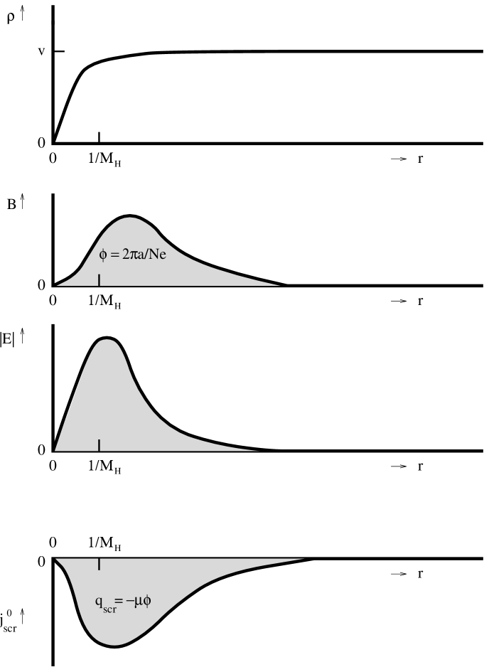
Figure 2.2: Qualitative behavior of the vortex solution carrying the quantized magnetic flux $\phi=\frac{2\pi a}{Ne}$ in the Chern-Simons limit. We have respectively depicted the modulus of the Higgs field $\rho$, the magnetic field $B$, the electric field $|{\mbox{\bf E}}|$ and the screening charge density $j^{0}_{\mbox{\scriptsize scr}}=-2(Ne)^{2}\rho^{2}A^{0}$ versus the radius $r$. The electromagnetic fields and the screening charge density vanish at $r=0$, reach there maximal value outside the core at $r=1/M_{H}$ and subsequently drop off exponentially with mass $M_{-}$ at larger distances.

An important issue is, of course, whether vortices will actually form or not, that is, whether the superconductor we are describing is type II or I respectively. In this context, the competition between the penetration depth $1/M_{-}$ of the electromagnetic fields and the coresize $1/M_{H}$ becomes important. In ordinary superconductors ($\mu=0$), an evaluation of the free energy yields that we are dealing with a type II superconductor if $M_{H}/M_{A}=\sqrt{\lambda}/Ne\geq 1$, and a type I superconductor otherwise [62]. Since $M_{-}$ is smaller then $M_{A}$, it is expected that in the presence of a Chern-Simons term the type II region is extended. A perturbative analysis for small topological mass $\mu$ shows that this is indeed the case [74]. In the following, we will always assume that our parameters are adjusted such that we are in the type II region.

Let us now briefly recall the structure of the electromagnetic fields of the vortex solution in the full range of parameters. To start with, the distribution of the magnetic field $B=\partial_{1}A^{2}-\partial_{2}A^{1}$ strongly depends on the topological mass $\mu$. For $\mu=0$, we are dealing with the Abrikosov-Nielsen-Olesen vortex discussed in section 1.3.2. In that case, the magnetic field reaches its maximal value at the center ($r=0$) of the vortex and drops off exponentially with mass $M_{A}$ at distances $r>1/M_{H}$. For $\mu\neq 0$, the magnetic field then decays exponentially with mass $M_{-}$ at distances $r>1/M_{H}$. Moreover, as the topological mass $|\mu|$ increases from zero, the magnetic field at the origin $r=0$ diminishes until it completely vanishes in the so-called Chern-Simons limit: $e,|\mu|\rightarrow\infty$, with fixed ratio $e^{2}/\mu$ [29]. (Note that in case the topological mass $\mu$ is quantized as (2.6.13), this limit simply means $e\rightarrow\infty$ leaving the Chern-Simons parameter $p$ fixed). Hence, in the Chern-Simons limit, which amounts to neglecting the Maxwell term in (2.6.2), the magnetic field is localized in a ring-shaped region around the core at $r=1/M_{H}$, as depicted in figure 2.2, see [29, 71, 74, 76, 77]. To proceed, as indicated by the zeroth component of the field equation (2.6.6), a magnetic field distribution $B$ generates an electric field distribution E iff $\mu\neq 0$. These electric fields are localized in a ring shaped region around the core at $1/M_{H}$ for all values of $\mu\neq 0$. To be specific, they vanish at $r=0$ and fall off with mass $M_{-}$ at distances $r>1/M_{H}$. We have seen in (2.6.25) how these electric fields, induced by the magnetic field of the vortex, are screened by the Chern-Simons Higgs medium occurring at $r>1/M_{H}$. A screening charge density $j_{\mbox{\scriptsize scr}}^{0}$ develops in the neighborhood of the core of the vortex, which falls off with mass $M_{-}$. In this static case, the screening charge density boils down to $j^{0}_{\mbox{\scriptsize scr}}=-M_{A}^{2}A^{0}$, that is, the Goldstone boson does not contribute. The analytical and numerical evaluations in for example [29, 71, 74, 76, 77] show that the distribution of $A_{0}$ is indeed of the shape described above.

The spin that can be calculated for this classical Chern-Simons vortex solution takes the value (e.g. [29, 71, 74, 76, 77])

$$s\;=\;\int d\,^{2}x\,\epsilon^{ij}x^{i}\,T^{0j}\;=\;\frac{\mu\phi^{2}}{4\pi},$$ (2.6.38)

where $T^{0j}$ denotes the energy momentum tensor. Note that this spin value is consistent with the quantum statistical parameter (2.6.28). That is, these vortices satisfy the spin statistics connection $\exp({\imath\Theta})=\exp({2\pi\imath s})$. This is actually a good point to resolve some inaccuracies in the literature. It is often stated (see for example [29, 71]) that it is the fact that the Chern-Simons vortices carry the charge (2.6.25) which leads to nontrivial Aharonov-Bohm interactions between these vortices. As we have argued, however, the screening charges $q_{\mbox{\scriptsize scr}}$ do not couple to the Aharonov-Bohm interactions [21] and the phases in (2.6.27), (2.6.28) are entirely due to the Chern-Simons term (2.6.4). In fact, erroneously assuming that the screening charges accompanying the vortices do couple to the Aharonov-Bohm interactions leads to the quantum statistical parameter $\exp(-\imath\mu\phi^{2}/2)$, which is inconsistent with the spin (2.6.38) carried by these vortices. In this respect, we remark that the correct quantum statistical parameter (2.6.28) for the vortices has also been derived in the dual formulation of this model [81].

To our knowledge, the nature of the static point charge solutions $j=(q\delta({\mbox{\bf x}}),0,0)$ of the field equations (2.6.17) have not been studied in the literature so far. An interesting question in this context is with which mass (2.6.20) the electromagnetic fields fall off around these matter charges. We conjecture that this exponential decay corresponds to the mass $M_{+}$. The overall picture then becomes that the magnetic vortices $\phi$ excite the $-$ polarization of the massive photon in the Chern-Simons Higgs medium, whereas the $+$ polarization is excited around the matter charges $q$.

2.6.3 ${\mbox{\bf Z}}_{N}$ Chern-Simons theory

Here, we turn to the incorporation of Dirac monopoles in the ${\mbox{\bf Z}}_{N}$ Chern-Simons Higgs phase discussed in the previous section. In other words, the topological mass is quantized as (2.6.13) in the following. We will argue that with this particular quantization, the ${\mbox{\bf Z}}_{N}$ Chern Simons theory describing the long distance physics in this Higgs phase corresponds to the 3-cocycle $\omega_{I}$ determined by the homomorphism (2.4.10) for this case [19, 20].

As we have seen in the previous section, the Higgs mechanism causes the identification of charge and flux occurring in unbroken Chern-Simons electrodynamics to disappear. That is, the spectrum of the ${\mbox{\bf Z}}_{N}$ Chern-Simons Higgs phase consists of the quantized matter charges $q=ne$, the quantized magnetic fluxes $\phi=\frac{2\pi a}{Ne}$ and dyonic combinations of the two. We will label these particles as $(a,n)$ with $a,n\in{\mbox{\bf Z}}$. Upon implementing the quantization (2.6.20) of the topological mass $\mu$, the Aharonov-Bohm interactions (2.6.26), (2.6.27) and (2.6.28) can be cast in the form

$${\cal R}^{2}\;|a,n\rangle|a^{\prime},n^{\prime}\rangle = e^{\frac{2\pi\imath}{N}(na^{\prime}+n^{\prime}a+\frac{2p}{N}aa^{\prime})}\;|a,n\rangle|a^{\prime},n^{\prime}\rangle$$ (2.6.39)

$${\cal R}\;|a,n\rangle|a,n\rangle = e^{\frac{2\pi\imath}{N}(na+\frac{p}{N}aa)}\;|a,n\rangle|a,n\rangle$$ (2.6.40)

$$T\;|a,n\rangle = e^{\frac{2\pi\imath}{N}(na+\frac{p}{N}aa)}\;|a,n\rangle.$$ (2.6.41)

Here, $p$ denotes the integral Chern-Simons parameter, while expression (2.6.41) contains the spins assigned to the particles. Under these remaining long range topological interactions, the charge label $n$ obviously becomes a ${\mbox{\bf Z}}_{N}$ quantum number, i.e. at large distances we are only able to distinguish the charges $n$ modulo $N$. Furthermore, in the presence of the Dirac monopoles/instantons (2.6.12) magnetic flux $a$ is conserved modulo $N$. However, the flux decay events are now accompanied by charge creation [18, 20]. To be specific, in terms of the integral flux and charge quantum numbers $a$ and $n$, the tunneling event induced by the minimal Dirac monopole can be recapitulated as

instanton: $$\left\{\begin{array}[]{lcl}a&\mapsto&a-N\\ n&\mapsto&n+2p.\end{array}\right.$$ (2.6.44)

We have depicted this effect of a Dirac monopole in the spectrum of a ${\mbox{\bf Z}}_{4}$ Chern-Simons Higgs phase in figure 2.3. Recall from section 2.6.1 that the quantization (2.6.13) of the topological mass was such that the particles connected by monopoles were invisible to the monodromies (2.6.8) and carried the same spin in the unbroken phase. This feature naturally persists in this broken phase. It is readily checked that the particles connected by the monopole (2.6.44) can not be distinguished by the Aharonov-Bohm interactions (2.6.39) and give rise to the same spin factor (2.6.41). As a result, the spectrum of this broken phase can be presented as

$$(a,n)\qquad\qquad\qquad\mbox{with}\qquad a,n\in 0,1,\ldots,N-1,$$ (2.6.45)

where it is understood that the modulo $N$ calculus for the magnetic fluxes $a$ involves the charge jump (2.6.44).

Figure 2.3: The spectrum of a ${\mbox{\bf Z}}_{4}$ Chern-Simons Higgs phase compactifies to the particles inside the dashed box. We depict the flux $\phi$ versus the matter charge $q$ and the screening charge $-q_{\mbox{\scriptsize scr}}=q+\mu\phi$ respectively. The Chern-Simons parameter $\mu$ is set to its minimal nontrivial value $\mu=\frac{e^{2}}{\pi}$, that is, $p=1$. The arrows visualize the tunneling event induced by a minimal Dirac monopole.

Let us now explicitly verify that we are indeed dealing with a ${\mbox{\bf Z}}_{N}$ gauge theory with Chern-Simons action (2.3.2), i.e.

$$\omega_{\mbox{\scriptsize I}}(a,b,c) = \exp\left(\frac{2\pi\imath p}{N^{2}}\,a(b+c-[b+c])\right),$$ (2.6.46)

where the rectangular brackets denote modulo $N$ calculus such that the sum always lies in the range $0,1,\ldots,N-1$. First of all, the different particles (2.6.45) constitute the compactified spectrum on which the quasi-quantum double $D^{\omega_{I}}({\mbox{\bf Z}}_{N})$ acts. The additional Aharonov-Bohm interactions among the fluxes are then absorbed in the definition of the dyon charges.  To be specific, the dyon charge (2.5.11) corresponding to the flux $a$ is given by

$${\alpha}(b) = \varepsilon_{a}(b)\;\Gamma^{n}(b),$$ (2.6.47)

with $\varepsilon_{a}(b)$ defined in (2.3.24)

$$\varepsilon_{a}(b) = \exp\left(\frac{2\pi\imath p}{N^{2}}ab\right),$$ (2.6.48)

and

$$\Gamma^{n}(b) = \exp\left(\frac{2\pi\imath}{N}nb\right),$$ (2.6.49)

an UIR of ${\mbox{\bf Z}}_{N}$. The action of the braid operator (2.5.19) now gives rise to the Aharonov-Bohm phases presented in (2.6.39) and (2.6.40), whereas the action of the central element (2.5.13) yields the spin factor (2.6.41). Furthermore, the fusion rules for $D^{\omega_{I}}({\mbox{\bf Z}}_{N})$ following from (2.5)

$$(a,n)\times(a^{\prime},n^{\prime}) = \left([a+a^{\prime}],[n+n^{\prime}+\frac{2p}{N}(a+a^{\prime}-[a+a^{\prime}])]\right),$$ (2.6.50)

express the tunneling properties of the Dirac monopoles. Specifically, iff the sum of the fluxes $a+a^{\prime}$ exceeds $N-1$, the composite carries unstable flux and tunnels back to the range (2.6.45) by means of the charged monopole (2.6.44). Note that the charge jump induced by the monopole for Chern-Simons parameter $p\neq 0$ implies that the fusion algebra now equals ${\mbox{\bf Z}}_{kN}\times{\mbox{\bf Z}}_{N/k}$ [48]. Here, we defined $k:=N/{\gcd}(p,N)$ for odd $N$ and $k:=N/{\gcd}(2p,N)$ for even $N$, where $\gcd$ stands for the greatest common divisor. In particular, for odd $N$ and Chern-Simons parameter $p=1$, the complete spectrum is generated by the single magnetic flux $a=1$. Finally, the charge conjugation operator ${\cal C}=S^{2}$ following from (2.5.30) takes the form

$${\cal C}\;(a,n) = \left([-a],[-n+\frac{2p}{N}(-a-[-a])]\right).$$ (2.6.51)

In other words, we have the usual action of the charge conjugation operator. The fluxes $a$ and charges $n$ reverse sign. Subsequently, the ‘twisted’ modulo $N$ calculus for the fluxes (2.6.44) and the ordinary modulo $N$ calculus for the charges are applied to return to the range (2.6.45). Also note that the particles and anti-particles in this theory naturally carry the same spin, that is, the action (2.6.41) of the modular $T$ matrix indeed commutes with ${\cal C}$.

Having established the fact that the $U(1)$ Chern-Simons term (2.6.4) gives rise to the 3-cocycle (2.6.46) in the residual ${\mbox{\bf Z}}_{N}$ gauge theory in the Higgs phase, we now turn to the periodicity $N$ of the Chern-Simons parameter $p$ as indicated by the homomorphism (2.4.10). This periodicity can be made explicit as follows. From the braid properties (2.6.39), the spin factors (2.6.41) and the fusion rules (2.6.50), we infer that setting the Chern-Simons parameter to $p=N$ amounts to an automorphism

$$(a,n) \longmapsto (a,[n+2a]),$$ (2.6.52)

of the spectrum (2.6.45) for $p=0$. In other words, for $p=N$ the theory describes the same topological interactions between the particles as for $p=0$, we just have relabeled the dyons.

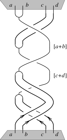
Figure 2.4: The 3-cocycle condition states that the topological action $\exp(\imath S_{\mbox{\scriptsize CSI}})$ for this process is trivial. The vertices in which the fluxes are fused correspond to a minimal Dirac instanton iff the total flux of the composite is larger then $N-1$.

Let us close this section by identifying the process corresponding to the Chern-Simons action (2.6.46). To start with, a comparison of the expressions (2.6.46) and (2.6.48) yields

$$\omega_{\mbox{\scriptsize I}}(a,b,c) = \varepsilon_{b}(a)\;\varepsilon_{c}(a)\;\varepsilon^{-1}_{[b+c]}(a),$$ (2.6.53)

from which we immediately conclude

$$\omega_{\mbox{\scriptsize I}}(a,b,c) = \exp(\imath S_{\mbox{\scriptsize CSI}})\left\{\vbox{\epsfbox{kocykle.eps}}\right\}\,.$$ (2.6.54)

Here, the fluxes $a$,$b$ and $c$ are again assumed to take values in the range $0,1,\ldots,N-1$. The vertex corresponding to fusion of the fluxes $b$ and $c$ then describes the tunneling event (2.6.44) induced by the minimal Dirac monopole iff the total flux $b+c$ of the composite exceeds $N-1$. Of course, the total Aharonov-Bohm phase for the process depicted in (2.6.54), which also involves the matter coupling (2.6.3), is trivial as witnessed by the fact that the quasitriangularity condition (2.5.21) is satisfied. The contribution (2.6.54) of the Chern-Simons term (2.6.4) to this total Aharonov-Bohm phase, however, is nontrivial iff the vertex corresponds to a monopole. It only generates Aharonov-Bohm phases between magnetic fluxes and therefore only notices the flux tunneling at the vertex and not the charge creation. Specifically, in the first braiding of the process (2.6.54), the Chern-Simons coupling generates the Aharonov-Bohm phase $\varepsilon_{b}(a)$, in the second $\varepsilon_{c}(a)$ and in the last $\varepsilon^{-1}_{[b+c]}(a)$. Hence, the total Chern-Simons action for this process indeed becomes (2.6.53). With the prescription (2.6.54), factorization of the topological action, the so-called skein relation

$$\exp(\imath S_{\mbox{\scriptsize CSI}})\left\{\vbox{\epsfbox{actie.eps}}\right\}\;=\;\exp(\imath S_{\mbox{\scriptsize CSI}})\left\{\vbox{\epsfbox{triv.eps}}\right\}\;=\;1,$$ (2.6.55)

and the obvious relation

$$\omega_{\mbox{\scriptsize I}}^{-1}(a,b,c) = \exp(\imath S_{\mbox{\scriptsize CSI}})\left\{\vbox{\epsfbox{kocinv.eps}}\right\}\,,$$ (2.6.56)

it is then readily verified that the 3-cocycle condition

$$\omega_{\mbox{\scriptsize I}}(a,b,c)\;\,\omega_{\mbox{\scriptsize I}}(a,[b+c],d)\;\,\omega_{\mbox{\scriptsize I}}^{-1}(a,b,[c+d])\;\,\omega_{\mbox{\scriptsize I}}^{-1}([a+b],c,d)\;\,\omega_{\mbox{\scriptsize I}}(b,c,d)\;=\;1\,,\qquad\;$$ (2.6.57)

boils down to the statement that the topological action $\exp(\imath S_{\mbox{\scriptsize CSI}})$ for the process depicted in figure 2.4 is trivial. In fact, this condition can now be interpreted as the requirement that the particles connected by Dirac monopoles should give rise to the same spin factor, which, in turn, imposes the quantization (2.6.13) of the topological mass. To that end, we first note that iff the total flux of either one of the particle pairs in figure 2.4 does not exceed $N-1$, i.e. $a+b<N-1$ and/or $c+d<N-1$, the 3-cocycle condition (2.6.57) is trivially satisfied, as follows from the skein relation (2.6.55). When both pairs carry flux larger then $N-1$, all vertices in figure 2.4 correspond to Dirac monopoles (2.6.44), transferring fluxes $N$ into the charges $2p$ and vice versa. The requirement that the action $\exp(\imath S_{\mbox{\scriptsize CSI}})$ for this process is trivial now becomes nonempty. Let us, for example, consider the case $a+b=N$ and $c+d=N$. Each pair may then be viewed as a single particle carrying either unstable flux $N$ or charge $2p$ depending on the vertex it has crossed. The total Chern-Simons action $\exp(\imath S_{\mbox{\scriptsize CSI}})$ for this case then reduces to the quantum statistical parameter (or spin factor) $\varepsilon_{N}(N)=\exp(2\pi\imath p)$ generated in the first braiding. Note that this Aharonov-Bohm phase is not cancelled by the one implied by the matter coupling (2.6.3) for this process. To be specific, this Aharonov-Bohm phase becomes $\exp(\imath S_{\mbox{\scriptsize matter}})=\exp(-4\pi\imath p)$ corresponding to the second braiding in figure 2.4 where the charge $2p$ is exchanged with the flux $N$ in a clockwise fashion. The last two braidings do not contribute. Upon demanding the total topological action $\exp(\imath S_{\mbox{\scriptsize CSI}}+\imath S_{\mbox{\scriptsize matter}})=\exp(-2\pi\imath p)$ to be trivial, we finally rederive the fact that the Chern-Simons parameter $p$ has to be integral. To conclude, the 3-cocycle condition (2.6.57) is necessary and sufficient for a consistent implementation of Dirac monopoles in a ${\mbox{\bf Z}}_{N}$ Chern-Simons gauge theory.

2.7 $U(1)\times U(1)$ Chern-Simons theory

The Chern-Simons terms (2.4.3) of type II establish pairwise couplings between the different $U(1)$ gauge fields $A^{(i)}_{\kappa}$ of a gauge group $U(1)^{k}$. Here, we discuss the simplest example of such a Chern-Simons theory of type II, namely that with gauge group $U(1)\times U(1)$ spontaneously broken down to the product of two cyclic groups ${\mbox{\bf Z}}_{N^{(1)}}\times{\mbox{\bf Z}}_{N^{(2)}}$. The generalization of the following analysis to $k>2$ is straightforward.

The spontaneously broken planar $U(1)\times U(1)$ Chern-Simons theory we consider is of the specific form

$$S = \int d\,^{3}x\;({\cal L}_{\mbox{\scriptsize YMH}}+{\cal L}_{\mbox{\scriptsize matter}}+{\cal L}_{\mbox{\scriptsize CSII}})$$ (2.7.1)

$${\cal L}_{\mbox{\scriptsize YMH}} = \sum_{i=1}^{2}\{-\frac{1}{4}F^{(i)\kappa\nu}F^{(i)}_{\kappa\nu}+({\cal D}^{\kappa}\Phi^{(i)})^{*}{\cal D}_{\kappa}\Phi^{(i)}-V(|\Phi^{(i)}|)\}$$ (2.7.2)

$${\cal L}_{\mbox{\scriptsize matter}} = -\sum_{i=1}^{2}j^{(i)\kappa}A^{(i)}_{\kappa}$$ (2.7.3)

$${\cal L}_{\mbox{\scriptsize CSII}} = \frac{\mu}{2}\epsilon^{\kappa\nu\tau}A^{(1)}_{\kappa}\partial_{\nu}A^{(2)}_{\tau},$$ (2.7.4)

where $A^{(1)}_{\kappa}$ and $A^{(2)}_{\kappa}$ denote the two different $U(1)$ gauge fields. We assume that these gauge symmetries are realized with quantized charges, that is, we are dealing with compact $U(1)$ gauge groups. To keep the discussion general, however, we allow for different fundamental charges for the two different compact gauge groups $U(1)$. The fundamental charge associated to the gauge field $A^{(1)}_{\kappa}$ is denoted by $e^{(1)}$, whereas $e^{(2)}$ is the fundamental charge for $A^{(2)}_{\kappa}$. The two Higgs fields $\Phi^{(1)}$ and $\Phi^{(2)}$ are assumed to carry charge $N^{(1)}e^{(1)}$ and $N^{(2)}e^{(2)}$ respectively, that is, ${\cal D}_{\kappa}\Phi^{(i)}=(\partial_{\kappa}+\imath N^{(i)}e^{(i)}A_{\kappa}^{(i)})\Phi^{(i)}$. The charges introduced by the matter currents $j^{(1)}$ and $j^{(2)}$ in (2.7.3), in turn, are quantized as $q^{(1)}=n^{(1)}e^{(1)}$ and $q^{(2)}=n^{(2)}e^{(2)}$ respectively with $n^{(1)},n^{(2)}\in{\mbox{\bf Z}}$. For convenience, both Higgs fields are endowed with the same (nonvanishing) vacuum expectation value $v$

$$V(|\Phi^{(i)}|) = \frac{\lambda}{4}(|\Phi^{(i)}|^{2}-v^{2})^{2}\qquad\qquad\lambda,v>0\qquad\mbox{and $i=1,2$.}$$ (2.7.5)

In other words, both compact $U(1)$ gauge groups are spontaneously broken down at the same energy scale $M_{H}=v\sqrt{2\lambda}$.

We proceed along the line of argument in the previous section. That is, we start with an analysis of the unbroken phase and present the argument for the quantization (2.4.7) of the topological mass $\mu$ in the presence of Dirac monopoles in section 2.7.1. In section 2.7.2, we then discuss the Chern-Simons Higgs screening mechanism in the broken phase and establish the Aharonov-Bohm interactions between the charges and magnetic fluxes in the spectrum. Finally, section 2.7.3 contains a study of the type II ${\mbox{\bf Z}}_{N^{(1)}}\times{\mbox{\bf Z}}_{N^{(2)}}$ Chern-Simons theory describing the long distance physics in the broken phase of this model.

2.7.1 Unbroken phase with Dirac monopoles

In this section, we turn to a brief discussion of the unbroken phase of the model (2.7.1), that is, we set $v=0$ and $\mu\neq 0$. For more detailed studies of this unbroken Chern-Simons theory, the interested reader is referred to [56, 65, 80, 128, 132] and the references given there.

Variation of the action (2.7.1) w.r.t. the gauge fields $A_{\kappa}^{(1)}$ and $A_{\kappa}^{(2)}$, respectively, gives rise to the following field equations

$$\begin{array}[]{lcl}\partial_{\nu}F^{(1)\;\nu\kappa}+\frac{\mu}{2}\epsilon^{\kappa\nu\tau}\partial_{\nu}A^{(2)}_{\tau}&=&j^{(1)\;\kappa}+j^{(1)\;\kappa}_{H}\\ \partial_{\nu}F^{(2)\;\nu\kappa}+\frac{\mu}{2}\epsilon^{\kappa\nu\tau}\partial_{\nu}A^{(1)}_{\tau}&=&j^{(2)\;\kappa}+j^{(2)\;\kappa}_{H}.\end{array}$$ (2.7.8)

with $j^{(i)}$ the two matter currents in (2.7.3) and $j^{(i)}_{H}$ the two Higgs currents in this model. This coupled set of differential equations leads to Klein-Gordon equations for the dual field strengths $\tilde{F}^{(1)}$ and $\tilde{F}^{(2)}$ with mass $|\mu|/2$. Thus the field strengths fall off exponentially and the Gauss’ laws take the form

$$\begin{array}[]{lcl}Q^{(1)}&=&q^{(1)}+q_{H}^{(1)}+\frac{\mu}{2}\phi^{(2)}\;=\;0\\ Q^{(2)}&=&q^{(2)}+q_{H}^{(2)}+\frac{\mu}{2}\phi^{(1)}\;=\;0,\end{array}$$ (2.7.11)

with

$$\begin{array}[]{ll}Q^{(i)}\;=\;\int\!d\,^{2}x\,\nabla\!\cdot\!\mbox{\bf E}^{(i)}\;=\;0,&\qquad\phi^{(i)}\;=\;\int\!d\,^{2}x\,\epsilon^{jk}\partial_{j}A^{(i)\;k}\\ q^{(i)}\;=\;\int\!d\,^{2}x\,j^{(i)\;0},&\qquad q_{H}^{(i)}\;=\;\int\!d\,^{2}x\,j^{(i)\;0}_{H}.\end{array}$$

Hence, the Chern-Simons screening mechanism operating in this theory attaches fluxes, which belong to one $U(1)$ gauge group, to the charges of the other [65, 132].

The long range interactions that remain between the particles in the spectrum of this model are the topological Aharonov-Bohm interactions implied by the couplings (2.7.3) and (2.7.4). These can be summarized as

$${\cal R}^{2}\;|q^{(1)},q^{(2)}\rangle|q^{(1)^{\prime}},q^{(2)^{\prime}}\rangle = e^{-\imath(\frac{2q^{(1)}q^{(2)^{\prime}}}{\mu}\,+\,\frac{2q^{(1)^{\prime}}q^{(2)}}{\mu})}\,|q^{(1)},q^{(2)}\rangle|q^{(1)^{\prime}},q^{(2)^{\prime}}\rangle$$ (2.7.13)

$${\cal R}\;|q^{(1)},q^{(2)}\rangle|q^{(1)},q^{(2)}\rangle = e^{-\imath\frac{2q^{(1)}q^{(2)}}{\mu}}\,|q^{(1)},q^{(2)}\rangle|q^{(1)},q^{(2)}\rangle.$$ (2.7.14)

From (2.7.14), we then conclude that the only particles endowed with a nontrivial spin are those that carry charges w.r.t. both $U(1)$ gauge groups. In other words, only these particles obey anyon statistics. The other particles are bosons.

Figure 2.5: Spectrum of unbroken $U(1)\times U(1)$ Chern-Simons theory of type II. We just depict the $q^{(1)}$ versus $\phi^{(2)}$ diagram. The topological mass $\mu$ is set to its minimal nontrivial value $\mu=\frac{e^{(1)}e^{(2)}}{\pi}$, i.e. $p=1$. The arrow represents the tunneling induced by a charged Dirac monopole/instanton $(2)$, which indicates that there are no stable particles in this theory for $p=1$. The charge/flux diagram for $q^{(2)}$ versus $\phi^{(1)}$ is obtained from this one by the replacement $(1)\leftrightarrow(2)$.

We proceed with the incorporation of Dirac monopoles/instantons in this compact Chern-Simons gauge theory. There are two different species associated to the two compact $U(1)$ gauge groups. The magnetic charges carried by these Dirac monopoles are quantized as $g^{(i)}=\frac{2\pi m^{(i)}}{e^{(i)}}$ with $m^{(i)}\in{\mbox{\bf Z}}$ and $i=1,2$. Given the coupling between the two $U(1)$ gauge fields established by the Chern-Simons term (2.7.4), the magnetic flux tunnelings induced by these monopoles in one $U(1)$ gauge group are accompanied by charge tunnelings in the other. Specifically, as indicated by the Gauss’ laws (2.7.11), the tunnelings associated with the two minimal Dirac monopoles become

instanton $$(1) \left\{\begin{array}[]{lcllcl}\Delta\phi^{(1)}&=&-\frac{2\pi}{e^{(1)}}\,,&\qquad\Delta\phi^{(2)}&=&0\\ \Delta q^{(1)}&=&0\,,&\qquad\Delta q^{(2)}&=&\mu\frac{\pi}{e^{(1)}}\end{array}\right.$$ : (2.7.17)

instanton $$(2) \left\{\begin{array}[]{lcllcl}\Delta\phi^{(1)}&=&0\,,&\qquad\;\Delta\phi^{(2)}&=&-\frac{2\pi}{e^{(2)}}\\ \Delta q^{(1)}&=&\mu\frac{\pi}{e^{(2)}}\,,&\qquad\;\Delta q^{(2)}&=&0.\end{array}\right.$$ : (2.7.20)

The presence of the Dirac monopole (2.7.17) implies quantization of the charges $q^{(1)}$ in multiples of $e^{(1)}$. This can be seen by the following simple argument. The tunneling event induced by the monopole (2.7.17) should be invisible to the long range monodromies involving the various charges in the spectrum of this theory. Hence, from (2.7.13) we infer that the Aharonov-Bohm phase $\exp(-\imath\frac{2q^{(1)}\Delta q^{(2)}}{\mu})=\exp(-\imath\frac{2\pi q^{(1)}}{e^{(1)}})$ should be trivial. Therefore, $q^{(1)}=n^{(1)}e^{(1)}$ with $n^{(1)}\in{\mbox{\bf Z}}$. In a similar fashion, we see that the presence of the Dirac monopole (2.7.20) leads to quantization of $q^{(2)}$ in multiples of $e^{(2)}$. Moreover, for consistency, the tunneling events induced by the monopoles should respect these quantization rules for $q^{(1)}$ and $q^{(2)}$. As follows from (2.7.17) and (2.7.20), this means that the topological mass is necessarily quantized as

$$\mu = \frac{pe^{(1)}e^{(2)}}{\pi}\qquad\qquad\mbox{with $p\in{\mbox{\bf Z}}$}.$$ (2.7.21)

It is easily verified that the consistency demand requiring the particles connected by Dirac monopoles to give rise to the same spin factor or quantum statistical parameter (2.7.14), does not lead to a further constraint on $\mu$ in this case.

To conclude, the spectrum of this unbroken $U(1)\times U(1)$ Chern-Simons theory, featuring Dirac monopoles, can be presented as in figure 2.5. The modulo calculus for the charges $q^{(1)}$ and $q^{(2)}$ induced by the Dirac monopoles (2.7.20) and (2.7.17), respectively, implies a compactification of the spectrum to $(p-1)^{2}$ different stable particles, with $p$ the integral Chern-Simons parameter in (2.7.21).

2.7.2 Higgs phase

We now switch on the Higgs mechanism by setting $v\neq 0$. At energies well below the symmetry breaking scale $M_{H}=v\sqrt{2\lambda}$ both Higgs fields $\Phi^{(i)}$ are then completely condensed

$$\Phi^{(i)}(x) \longmapsto v\exp(\imath\sigma^{(i)}(x))\qquad\mbox{for $i=1,2.$}$$ (2.7.22)

Hence, the dynamics of the Chern-Simons Higgs medium in this model is described by the effective action obtained from the following simplification in (2.7.1)

$$({\cal D}^{\kappa}\Phi^{(i)})^{*}{\cal D}_{\kappa}\Phi^{(i)}-V(|\Phi^{(i)}|) \longmapsto \frac{M_{A}^{(i)\,2}}{2}\tilde{A}^{(i)\;\kappa}\tilde{A}^{(i)}_{\kappa}\qquad\qquad$$ (2.7.23)

$$\tilde{A}^{(i)}_{\kappa} := A^{(i)}_{\kappa}+\frac{1}{N^{(i)}e^{(i)}}\partial_{\kappa}\sigma^{(i)}\qquad\qquad$$

$$M_{A}^{(i)} = N^{(i)}e^{(i)}v\sqrt{2},\qquad\qquad$$

with $i=1,2$. A derivation similar to the one for (2.6.20) reveals that the two polarizations $+$ and $-$ of the photon fields $\tilde{A}^{(i)}_{\kappa}$ acquire masses $M^{(i)}_{\pm}$, which differ by the topological mass $|\mu|/2$. We refrain from giving the explicit expressions of the masses $M^{(i)}_{\pm}$ in terms of $\mu$, $M_{A}^{(1)}$ and $M_{A}^{(2)}$.

In this broken phase, the Higgs currents $j_{H}^{(i)}$ appearing in the field equations (2.7.8) become screening currents $j_{\mbox{\scriptsize scr}}^{(i)}$

$$j_{H}^{(i)} \longmapsto j_{\mbox{\scriptsize scr}}^{(i)}\;:=\;-M_{A}^{(i)\,2}\tilde{A}^{(i)}.$$ (2.7.24)

In particular, the Gauss’ laws (2.7.11) now take the form

$$\begin{array}[]{lcl}Q^{(1)}&=&q^{(1)}+q_{\mbox{\scriptsize scr}}^{(1)}+\frac{\mu}{2}\phi^{(2)}\;=\;0\\ Q^{(2)}&=&q^{(2)}+q_{\mbox{\scriptsize scr}}^{(2)}+\frac{\mu}{2}\phi^{(1)}\;=\;0,\end{array}$$ (2.7.27)

with

$$q_{\mbox{\scriptsize scr}}^{(i)} := \int\!d\,^{2}x\,j^{(i)\,0}_{\mbox{\scriptsize scr}}.$$ (2.7.28)

As we have seen in section 2.6.2, the emergence of the screening charges (2.7.28) is at the heart of the de-identification of charge and flux occurring in the phase transition from the unbroken phase to the broken phase in a Chern-Simons gauge theory. They accompany the matter charges $q^{(i)}$ provided by the currents $j^{(i)}$ as well as the magnetic vortices.

Let us first focus on the magnetic vortices in this model. There are two different species associated with the winding of the two different Higgs fields $\Phi^{(1)}$ and $\Phi^{(2)}$. These vortices, which are of characteristic size $1/M_{H}$, carry the quantized magnetic fluxes

$$\phi^{(i)} = \frac{2\pi a^{(i)}}{N^{(i)}e^{(i)}}\qquad\mbox{with $a^{(i)}\in{\mbox{\bf Z}}$.}$$ (2.7.29)

As indicated by the Gauss’ laws (2.7.27), these vortices induce screening charges in the Higgs medium

$$\begin{array}[]{lcl}q_{\mbox{\scriptsize scr}}^{(1)}&=&-\frac{\mu}{2}\phi^{(2)}\\ q_{\mbox{\scriptsize scr}}^{(2)}&=&-\frac{\mu}{2}\phi^{(1)},\end{array}$$

which completely screen the Coulomb fields generated by their magnetic fluxes. The screening charges do not couple to the Aharonov-Bohm interactions. Therefore, the long range Aharonov-Bohm interactions among the vortices implied by the Chern-Simons coupling (2.7.4) are not screened

$${\cal R}^{2}\;|\phi^{(1)},\phi^{(2)}\rangle|\phi^{(1)^{\prime}},\phi^{(2)^{\prime}}\rangle = e^{\imath\frac{\mu}{2}(\phi^{(1)}\phi^{(2)^{\prime}}+\,\phi^{(1)^{\prime}}\phi^{(2)})}\,|\phi^{(1)},\phi^{(2)}\rangle|\phi^{(1)^{\prime}},\phi^{(2)^{\prime}}\rangle$$ (2.7.31)

$${\cal R}\;|\phi^{(1)},\phi^{(2)}\rangle|\phi^{(1)},\phi^{(2)}\rangle = e^{\imath\frac{\mu}{2}\phi^{(1)}\phi^{(2)}}\,|\phi^{(1)},\phi^{(2)}\rangle|\phi^{(1)},\phi^{(2)}\rangle.$$ (2.7.32)

Note that there are no Aharonov-Bohm phases generated among vortices of the same species. Thus there is only a nontrivial spin assigned to composites carrying flux w.r.t. both broken $U(1)$ gauge groups.

Finally, the matter charges $q^{(i)}$ provided by the currents $j^{(i)}$ induce the screening charges $q_{\mbox{\scriptsize scr}}^{(i)}=-q^{(i)}$ in the Higgs medium, screening their Coulomb interactions, but not their Aharonov-Bohm interactions with the vortices. The remaining long range interactions for these charges can then be summarized by

$${\cal R}^{2}\;|q^{(1)},q^{(2)}\rangle|\phi^{(1)},\phi^{(2)}\rangle = e^{\imath(q^{(1)}\phi^{(1)}+\,q^{(2)}\phi^{(2)})}\,|q^{(1)},q^{(2)}\rangle|\phi^{(1)},\phi^{(2)}\rangle,$$ (2.7.33)

as implied by the matter coupling (2.7.3).

2.7.3 ${\mbox{\bf Z}}_{N^{(1)}}\times{\mbox{\bf Z}}_{N^{(2)}}$ Chern-Simons theory of type II

The discussion in the previous section, in fact, pertains to all values of the topological mass $\mu$. Here, we again assume that the model features the Dirac monopoles (2.7.17) and (2.7.20), which implies the quantization (2.7.21) of $\mu$. We will show that under these circumstances the long distance physics of the Higgs phase is described by a ${\mbox{\bf Z}}_{N^{(1)}}\times{\mbox{\bf Z}}_{N^{(2)}}$ gauge theory with a 3-cocycle $\omega_{\mbox{\scriptsize II}}$ of type II determined by the homomorphism (2.4.11).

Let us first recall from the previous section that the spectrum of the ${\mbox{\bf Z}}_{N^{(1)}}\times{\mbox{\bf Z}}_{N^{(2)}}$ Chern-Simons Higgs phase consists of the matter charges $q^{(i)}=n^{(i)}e^{(i)}$, the quantized magnetic fluxes (2.7.29) and the dyonic combinations. We will label these particles as $\left(A,n^{(1)}n^{(2)}\right)$ with $A:=(a^{(1)},a^{(2)})$ and $a^{(i)},n^{(i)}\in{\mbox{\bf Z}}$. Upon implementing (2.7.21), the Aharonov-Bohm interactions (2.7.31), (2.7.32) and (2.7.33) between these particles can then be recapitulated as

$${\cal R}^{2}\;|A,n^{(1)}n^{(2)}\rangle|A^{\prime},n^{(1)^{\prime}}n^{(2)^{\prime}}\rangle = \alpha^{\prime}(A)\;\alpha(A^{\prime})\;|A,n^{(1)}n^{(2)}\rangle|A^{\prime},n^{(1)^{\prime}}n^{(2)^{\prime}}\rangle\qquad$$ (2.7.34)

$${\cal R}\;|A,n^{(1)}n^{(2)}\rangle|A,n^{(1)}n^{(2)}\rangle = \alpha(A)\;|A,n^{(1)}n^{(2)}\rangle|A,n^{(1)}n^{(2)}\rangle$$ (2.7.35)

$$T\;|A,n^{(1)}n^{(2)}\rangle = \alpha(A)\;|A,n^{(1)}n^{(2)}\rangle,$$ (2.7.36)

with

$$\alpha(A^{\prime}) := \varepsilon_{A}(A^{\prime})\;\Gamma^{n^{(1)}n^{(2)}}(A^{\prime})$$ (2.7.37)

$$\alpha^{\prime}(A) := \varepsilon_{A^{\prime}}(A)\;\Gamma^{n^{(1)^{\prime}}n^{(2)^{\prime}}}(A).$$ (2.7.38)

Here

$$\Gamma^{n^{(1)}n^{(2)}}(A) = \exp\left(\frac{2\pi\imath}{N^{(1)}}\,n^{(1)}a^{(1)}+\frac{2\pi\imath}{N^{(2)}}\,n^{(2)}a^{(2)}\right),$$ (2.7.39)

denotes an UIR of the group ${\mbox{\bf Z}}_{N^{(1)}}\times{\mbox{\bf Z}}_{N^{(2)}}$, whereas the epsilon factors are identical to (2.3.25), that is

$$\varepsilon_{A}(A^{\prime}) = \exp\left(\frac{2\pi\imath p}{N^{(1)}N^{(2)}}\,a^{(1)}a^{(2)^{\prime}}\right),$$ (2.7.40)

with $p$ the integral Chern-Simons parameter in (2.7.21). Under these remaining long range Aharonov-Bohm interactions, the charge labels $n^{(i)}$ clearly become ${\mbox{\bf Z}}_{N^{(i)}}$ quantum numbers. Moreover, in the presence of the Dirac monopoles (2.7.17) and (2.7.20) the fluxes $a^{(i)}$ are conserved modulo $N^{(i)}$. Specifically, in terms of the integral charge and flux quantum numbers $n^{(i)}$ and $a^{(i)}$ the tunneling events corresponding to these minimal monopoles read

instanton $$(1) \left\{\begin{array}[]{lcl}a^{(1)}&\mapsto&a^{(1)}-N^{(1)}\\ n^{(2)}&\mapsto&n^{(2)}+p\end{array}\right.$$ : (2.7.43)

instanton $$(2) \left\{\begin{array}[]{lcl}a^{(2)}&\mapsto&a^{(2)}-N^{(2)}\\ n^{(1)}&\mapsto&n^{(1)}+p\,.\end{array}\right.$$ : (2.7.46)

Here, we substituted (2.7.21) in (2.7.17) and (2.7.20) respectively. Hence, the decay of an unstable flux corresponding to one residual cyclic gauge group is accompanied by the creation of the charge $p$ w.r.t. the other cyclic gauge group. See also figure 2.6. It is again easily verified that these local tunneling events are invisible to the long range Aharonov-Bohm interactions (2.7.34) and that the particles connected by the monopoles exhibit the same spin factor (2.7.36). The conclusion then becomes that the spectrum of a ${\mbox{\bf Z}}_{N^{(1)}}\times{\mbox{\bf Z}}_{N^{(2)}}$ Higgs phase corresponding to an integral Chern-Simons parameter $p$ compactifies to

$$\left(A,n^{(1)}n^{(2)}\right)\qquad\qquad\mbox{with $A=(a^{(1)},a^{(2)})$ and $a^{(i)},n^{(i)}\in 0,1,\ldots,N^{(i)}-1$},\qquad$$ (2.7.47)

where the modulo calculus for the flux quantum numbers $a^{(i)}$ involves the charge jumps displayed in (2.7.43) and (2.7.46).

Figure 2.6: The spectrum of a Higgs phase with residual gauge group ${\mbox{\bf Z}}_{2}\times{\mbox{\bf Z}}_{4}$ and Chern-Simons action of type II compactifies to the particles in the dashed boxes. We have displayed the flux $\phi^{(2)}$ versus the charge $q^{(1)}$ and the flux $\phi^{(1)}$ versus the charge $q^{(2)}$. Here, the topological mass is assumed to take its minimal nontrivial value $\mu=\frac{e^{(1)}e^{(2)}}{\pi}$, that is,  $p=1$. The arrows in figure (a) and (b) visualize the tunnelings corresponding to the Dirac monopole (2) and the monopole (1) respectively.

It is now readily checked that in accordance with the homomorphism (2.4.11) for this case, the ${\mbox{\bf Z}}_{N^{(1)}}\times{\mbox{\bf Z}}_{N^{(2)}}$ gauge theory labeled by the integral Chern-Simons parameter $p$ corresponds to the 3-cocycle of type II given in (2.3.20), which we repeat for convenience

$$\omega_{\mbox{\scriptsize II}}(A,B,C) = \exp\left(\frac{2\pi\imath p}{N^{(1)}N^{(2)}}\;a^{(1)}(b^{(2)}+c^{(2)}-[b^{(2)}+c^{(2)}])\right).$$ (2.7.48)

In other words, the spectrum (2.7.47) with the topological interactions summarized in the expressions (2.7.34), (2.7.35) and (2.7.36) is governed by the quasi-quantum double $D^{\omega_{\mbox{\tiny II}}}({\mbox{\bf Z}}_{N^{(1)}}\times{\mbox{\bf Z}}_{N^{(2)}})$ with $\omega_{\mbox{\scriptsize II}}$ the 3-cocycle (2.7.48). In particular, the fusion rules following from (2.5)

$$\left(A,n^{(1)}n^{(2)}\right)\times\left(A^{\prime},n^{(1)^{\prime}}n^{(2)^{\prime}}\right) = \left([A+A^{\prime}],n_{sum}^{(1)}n_{sum}^{(2)}\right),$$ (2.7.49)

with

$$[A+A^{\prime}] = ([a^{(1)}+a^{(1)^{\prime}}],[a^{(2)}+a^{(2)^{\prime}}])$$

$$n_{sum}^{(1)} = [n^{(1)}+n^{(1)^{\prime}}+\frac{p}{N^{(2)}}(a^{(2)}+a^{(2)^{\prime}}-[a^{(2)}+a^{(2)^{\prime}}])]$$

$$n_{sum}^{(2)} = [n^{(2)}+n^{(2)^{\prime}}+\frac{p}{N^{(1)}}(a^{(1)}+a^{(1)^{\prime}}-[a^{(1)}+a^{(1)^{\prime}}])],$$

are again a direct reflection of the tunneling properties induced by the monopoles (2.7.17) and (2.7.20). Note that these ‘twisted’ tunneling properties actually imply that the complete spectrum (2.7.47) of this theory is just generated by the two fluxes $a^{(1)}=1$ and $a^{(2)}=1$, if the Chern-Simons parameter $p$ is set to $1$.

To conclude, at first sight the periodicity $\gcd(N^{(1)},N^{(2)})$ in the Chern-Simons parameter $p$ as indicated by the mapping (2.4.11) is not completely obvious from the fusion rules (2.6.50) and the topological interactions (2.7.34), (2.7.35) and (2.7.36). Here, we recall theorem (2.3.22), which was the crucial ingredient in the proof that the 3-cocycle (2.7.48) boils down to a 3-coboundary for $p=\gcd(N^{(1)},N^{(2)})$. We then simply infer that setting the Chern-Simons parameter $p$ to $\gcd(N^{(1)},N^{(2)})$ amounts to the automorphism

$$\left(A,n^{(1)}n^{(2)}\right) \longmapsto \left(A,[n^{(1)}+xa^{(2)}][n^{(2)}+ya^{(1)}]\right),$$

of the spectrum (2.7.47) for $p=0$, where $x$ and $y$ are the integers appearing in (2.3.22). Hence, the theories for $p=0$ and $p=\gcd(N^{(1)},N^{(2)})$ are the same up to a relabeling of the dyons.

2.8 ${\mbox{\bf Z}}_{2}\times{\mbox{\bf Z}}_{2}\times{\mbox{\bf Z}}_{2}$ Chern-Simons theory

Chern-Simons actions (2.3.21) of type III occur for finite abelian gauge groups ${H}$ corresponding to direct products of three or more cyclic groups. As indicated by the homomorphism (2.2.5), such type III Chern-Simons theories do not emerge in spontaneously broken $U(1)^{k}$ Chern-Simons theories. At present, it is not clear to us whether there actually exist symmetry breaking schemes which give rise to 3-cocycles of type III for a residual finite abelian gauge group in the Higgs phase. This point deserves further scrutiny especially since adding a type III Chern-Simons action to an abelian discrete $H$ gauge theory has some drastic consequences. It renders such a theory nonabelian. In general these type III Chern-Simons theories are, in fact, dual versions of gauge theories featuring a finite nonabelian gauge group.

Here, we just focus on the simplest example of a type III Chern-Simons theory, namely that with gauge group ${H}\simeq{\mbox{\bf Z}}_{2}\times{\mbox{\bf Z}}_{2}\times{\mbox{\bf Z}}_{2}$. The generalization to other abelian groups allowing for 3-cocycles of type III is straightforward. The outline is as follows. In section 2.8.1, we will show that the incorporation of the type III Chern-Simons action in a ${\mbox{\bf Z}}_{2}\times{\mbox{\bf Z}}_{2}\times{\mbox{\bf Z}}_{2}$ gauge theory involves a ‘collapse’ of the spectrum. Whereas the ordinary ${\mbox{\bf Z}}_{2}\times{\mbox{\bf Z}}_{2}\times{\mbox{\bf Z}}_{2}$ theory features 64 different singlet particles, the spectrum just consists of 22 different particles in the presence of the 3-cocycle of type III. Specifically, the dyon charges, which formed one dimensional UIR’s of ${\mbox{\bf Z}}_{2}\times{\mbox{\bf Z}}_{2}\times{\mbox{\bf Z}}_{2}$, are reorganized into two dimensional or doublet projective representations of ${\mbox{\bf Z}}_{2}\times{\mbox{\bf Z}}_{2}\times{\mbox{\bf Z}}_{2}$. This abelian gauge theory then describes nonabelian topological interactions between these doublet dyons, which will be discussed in section 2.8.2. In section 2.8.3, we finally establish that this theory is a dual version of the ordinary discrete gauge theory with nonabelian gauge group the dihedral group $D_{4}$. Furthermore, we show that upon adding a type I Chern-Simons action, the theory actually becomes dual to the $\bar{D}_{2}$ gauge theory discussed in section 1.6.

2.8.1 Spectrum

The type III Chern-Simons action (2.3.2) for the gauge group ${\mbox{\bf Z}}_{2}\times{\mbox{\bf Z}}_{2}\times{\mbox{\bf Z}}_{2}$ takes the form

$$\omega_{\mbox{\scriptsize III}}(A,B,C) = \exp\left(\pi\imath\,a^{(1)}b^{(2)}c^{(3)}\right),$$ (2.8.1)

where we have set the integral cocycle parameter to its nontrivial value, that is, $p_{\mbox{\scriptsize III}}=1$. From the slant product (2.3.10) as applied to the 3-cocycle (2.8.1), we infer that the 2-cocycle $c_{A}$, which enters the definition of the projective ${\mbox{\bf Z}}_{2}\times{\mbox{\bf Z}}_{2}\times{\mbox{\bf Z}}_{2}$ dyon charge representations (2.3.11) for the magnetic flux $A$ in this Chern-Simons theory, reads

$$c_{A}(B,C) = \exp\left(\pi\imath\{a^{(1)}b^{(2)}c^{(3)}+b^{(1)}c^{(2)}a^{(3)}-b^{(1)}a^{(2)}c^{(3)}\}\right).$$ (2.8.2)

For the trivial magnetic flux sector $A=0$, this 2-cocycle naturally vanishes, so the pure charges are given by the ordinary UIR’s of ${\mbox{\bf Z}}_{2}\times{\mbox{\bf Z}}_{2}\times{\mbox{\bf Z}}_{2}$. For the nontrivial magnetic flux sectors $A\neq 0$, the 2-cocycle $c_{A}$ is nontrivial, that is, it can not be decomposed as (2.3.23). Hence, we are dealing with projective representations that can not be obtained from ordinary representations by the inclusion of extra Aharonov-Bohm phases $\varepsilon$ as in (2.5.11). An important result in projective representation theory now states that for a given finite group ${H}$ the number of inequivalent irreducible projective representations (2.3.11) associated with a 2-cocycle $c$ equals the number of $c$-regular classes in ${H}$ [78]. Here, an element $h\in{H}$ is called c-regular iff $c(h,g)=c(g,h)$ for all $g\in{H}$. If $h$ is c-regular, so are all its conjugates. In our abelian example with the 2-cocycle $c_{A}$ for $A\neq 0$, it is easily verified that there are only two $c_{A}$ regular classes in ${\mbox{\bf Z}}_{2}\times{\mbox{\bf Z}}_{2}\times{\mbox{\bf Z}}_{2}$, namely the trivial flux $0$ and $A$ itself. Hence, there are only two inequivalent irreducible projective representations associated with $c_{A}$. Just as for ordinary UIR’s, the sum of the squares of the dimensions of these projective UIR’s should equal the order 8 of the group ${\mbox{\bf Z}}_{2}\times{\mbox{\bf Z}}_{2}\times{\mbox{\bf Z}}_{2}$ and we find that both representations are two dimensional. An explicit construction of these representations can be found in [78].

Let us illustrate these general remarks by considering the effect of the presence of the 2-cocycle $c_{A}$ for the particular magnetic flux $A=100$. Substituting (2.8.2) in (2.3.11) yields the following set of defining relations for the generators of ${\mbox{\bf Z}}_{2}\times{\mbox{\bf Z}}_{2}\times{\mbox{\bf Z}}_{2}$ in the projective representation $\alpha$

$$\begin{array}[]{rcl}\alpha(100)^{2}&=&\alpha(010)^{2}\;=\;\alpha(001)^{2}\;=\;{\mbox{\bf 1}}\\ \alpha(100)\,\cdot\,\alpha(010)&=&\alpha(010)\,\cdot\,\alpha(100)\\ \alpha(100)\,\cdot\,\alpha(001)&=&\alpha(001)\,\cdot\,\alpha(100)\\ \alpha(010)\,\cdot\,\alpha(001)&=&-\alpha(001)\,\cdot\,\alpha(010).\end{array}$$ (2.8.7)

In other words, the generators $\alpha(010)$ and $\alpha(001)$ become anti-commuting, which indicates that the projective representation $\alpha$ is necessarily higher dimensional. Specifically, the two inequivalent two dimensional projective UIR’s associated to the 2-cocycle $c_{100}$ are given by [78]

$$\alpha^{1}_{\pm}(100)=\pm\left(\begin{array}[]{rr}1&0\\ 0&1\end{array}\right),\qquad\alpha^{1}_{\pm}(010)=\left(\begin{array}[]{rr}0&1\\ 1&0\end{array}\right),\qquad\alpha^{1}_{\pm}(001)=\left(\begin{array}[]{rr}1&0\\ 0&-1\end{array}\right).$$ (2.8.8)

Here, the subscript $+$ and $-$ labels the two inequivalent representations, whereas the superscript $1$ refers to the fact that $A=100$ denotes the nontrivial magnetic flux associated to the first gauge group ${\mbox{\bf Z}}_{2}$ in the product ${\mbox{\bf Z}}_{2}\times{\mbox{\bf Z}}_{2}\times{\mbox{\bf Z}}_{2}$. In passing, we note that the set of matrices (2.8.8) generates the two dimensional UIR of the dihedral point group $D_{4}$.

It is instructive to examine the projective representations in (2.8.8) a little closer. In an ordinary ${\mbox{\bf Z}}_{2}\times{\mbox{\bf Z}}_{2}\times{\mbox{\bf Z}}_{2}$ gauge theory, the three global ${\mbox{\bf Z}}_{2}$ symmetry generators commute with each other and with the flux projection operators. Thus the total internal Hilbert space of this gauge theory allows for a basis of mutual eigenvectors $|A,n^{(1)}n^{(2)}n^{(3)}\rangle$, where the labels $n^{(i)}\in 0,1$ denote the ${\mbox{\bf Z}}_{2}$ representations and $A\in{\mbox{\bf Z}}_{2}\times{\mbox{\bf Z}}_{2}\times{\mbox{\bf Z}}_{2}$ the different magnetic fluxes. In other words, the spectrum consists of 64 different particles each carrying a one dimensional internal Hilbert space labeled by a flux and a charge. Upon introducing the type III Chern-Simons action (2.8.1) in this abelian discrete gauge theory, the global ${\mbox{\bf Z}}_{2}$ symmetry generators cease to commute with each other as we have seen explicitly for the flux sector $A=100$ in (2.8.7). In this sector, the eigenvectors of the two non-commuting ${\mbox{\bf Z}}_{2}$ generators are rearranged into an irreducible doublet representation. We can, however, still diagonalize the generators in this doublet representation separately to uncover the ${\mbox{\bf Z}}_{2}$ eigenvalues $1$ and $-1$. Hence, the ${\mbox{\bf Z}}_{2}$ charge quantum numbers $n^{(i)}\in 0,1$ remain unaltered in the presence of a Chern-Simons action of type III.

The analysis is completely similar for the other flux sectors. First of all, the two 2-dimensional projective dyon charge representations $\alpha^{2}_{\pm}$ associated with the magnetic flux $A=010$ follow from a cyclic permutation of the set of matrices in (2.8.8), such that the diagonal matrix $\pm{\mbox{\bf 1}}$ ends up at the second position, that is, $\alpha^{2}_{\pm}(010)=\pm{\mbox{\bf 1}}$. The two projective representations $\alpha^{3}_{\pm}$ for $A=001$ are then defined by the cyclic permutation of the matrices in (2.8.8) fixed by $\alpha^{3}_{\pm}(001)=\pm{\mbox{\bf 1}}$. To proceed, the two 2-dimensional projective representations $\beta_{\pm}^{1}$ for the flux $A=011$ are determined by

$$\beta^{1}_{\pm}(100)=\left(\begin{array}[]{rr}1&0\\ 0&-1\end{array}\right),\qquad\beta^{1}_{\pm}(010)=\left(\begin{array}[]{rr}0&1\\ 1&0\end{array}\right),\qquad\beta^{1}_{\pm}(001)=\pm\left(\begin{array}[]{rr}0&1\\ 1&0\end{array}\right).$$ (2.8.9)

Here, the subscript $+$ and $-$ again labels the two inequivalent representations, while the superscript now reflects the fact that $A=011$ corresponds to a trivial flux w.r.t. to the first gauge group ${\mbox{\bf Z}}_{2}$ in the product ${\mbox{\bf Z}}_{2}\times{\mbox{\bf Z}}_{2}\times{\mbox{\bf Z}}_{2}$. The two representations $\beta_{\pm}^{2}$ associated to the flux $A=101$ are defined by the same set of matrices (2.8.9) moved one step to the right with cyclic boundary conditions, whereas the representations $\beta_{\pm}^{3}$ for $A=110$ are given by the same set moved two steps to the right with cyclic boundary conditions. Finally, the two inequivalent dyon charge representations $\gamma_{\pm}$ for the magnetic flux $A=111$ are generated by the Pauli matrices

$$\gamma_{\pm}(100)=\pm\left(\begin{array}[]{rr}0&1\\ 1&0\end{array}\right),\;\gamma_{\pm}(010)=\pm\left(\begin{array}[]{rr}0&-\imath\\ \imath&0\end{array}\right),\;\gamma_{\pm}(001)=\pm\left(\begin{array}[]{rr}1&0\\ 0&-1\end{array}\right).$$ (2.8.10)

In contrast with the sets of matrices contained in (2.8.8) and (2.8.9) which generate the 2-dimensional representation of the dihedral group $D_{4}$, the two sets in (2.8.10) generate the two dimensional UIR’s of the truncated pure braid group $P(3,4)$ displayed in the character table 1.5 of appendix 1.B.

The complete spectrum of this ${\mbox{\bf Z}}_{2}\times{\mbox{\bf Z}}_{2}\times{\mbox{\bf Z}}_{2}$ Chern-Simons theory of type III can now be summarized as

$$\begin{array}[]{cc}\mbox{particle}&\qquad\exp(2\pi\imath s)\\ &\\ (0,n^{(1)}n^{(2)}n^{(3)})&\qquad 1\\ (100,\alpha^{1}_{\pm}),\,(010,\alpha^{2}_{\pm}),\,(001,\alpha^{3}_{\pm})&\qquad\pm 1\\ (011,\beta^{1}_{\pm}),\,(101,\beta^{2}_{\pm}),\,(110,\beta^{3}_{\pm})&\qquad\pm 1\\ (111,\gamma_{\pm})&\qquad\mp\imath,\end{array}$$ (2.8.11)

where the spin factors for the particles are obtained from the action of the flux of the particle on its own dyon charge as indicated by expression (2.5.15). Hence, there are 7 nontrivial pure charges $(0,n^{(1)}n^{(2)}n^{(3)})$ labeled by the ordinary nontrivial one dimensional ${\mbox{\bf Z}}_{2}\times{\mbox{\bf Z}}_{2}\times{\mbox{\bf Z}}_{2}$ representations (2.5.12). The trivial representation naturally corresponds to the vacuum. In addition, there are 14 dyons carrying a nontrivial abelian magnetic flux and a doublet charge. The conclusion then becomes that the introduction of a Chern-Simons action of type III leads to a compactification or ‘collapse’ of the spectrum. Whereas an ordinary ${\mbox{\bf Z}}_{2}\times{\mbox{\bf Z}}_{2}\times{\mbox{\bf Z}}_{2}$ gauge theory features 64 different singlet particles, we only have 22 distinct particles in the presence of a type III Chern-Simons action (2.8.1). To be specific, the singlet dyon charges are rearranged into doublets so that the squares of the dimensions of the internal Hilbert spaces for the particles in the spectrum still add up to the order of the quasi-quantum double $D^{\omega_{\mbox{\tiny III}}}({\mbox{\bf Z}}_{2}\times{\mbox{\bf Z}}_{2}\times{\mbox{\bf Z}}_{2})$, that is, $8^{2}=8\cdot 1^{2}+14\cdot 2^{2}$. Let us close with the remark that this collapse of the spectrum can also be seen directly by evaluating the Dijkgraaf-Witten invariant for the 3-torus $S^{1}\times S^{1}\times S^{1}$ with the 3-cocycle (2.8.1). See section 2.9 in this connection.

2.8.2 Nonabelian topological interactions

Here, we highlight the nonabelian nature of the topological interactions in this type III Chern-Simons theory with abelian gauge group ${\mbox{\bf Z}}_{2}\times{\mbox{\bf Z}}_{2}\times{\mbox{\bf Z}}_{2}$.

Let us start by considering the Aharonov-Bohm scattering experiment, depicted in figure 1.13 of appendix 1.A, in which the incoming projectile now is the dyon $(100,\alpha_{+}^{1})$, while the dyon $(011,\beta^{1}_{+})$ plays the role of the scatterer. We choose the following flux/charge eigenbasis for the four dimensional internal Hilbert space describing this 2-dyon system

$$e_{\uparrow\uparrow} = |100,\left(\begin{array}[]{c}1\\ 0\end{array}\right)\rangle\otimes|011,\left(\begin{array}[]{c}1\\ 0\end{array}\right)\rangle$$ (2.8.16)

$$e_{\downarrow\uparrow} = |100,\left(\begin{array}[]{c}0\\ 1\end{array}\right)\rangle\otimes|011,\left(\begin{array}[]{c}1\\ 0\end{array}\right)\rangle$$ (2.8.21)

$$e_{\uparrow\downarrow} = |100,\left(\begin{array}[]{c}1\\ 0\end{array}\right)\rangle\otimes|011,\left(\begin{array}[]{c}0\\ 1\end{array}\right)\rangle$$ (2.8.26)

$$e_{\downarrow\downarrow} = |100,\left(\begin{array}[]{c}0\\ 1\end{array}\right)\rangle\otimes|011,\left(\begin{array}[]{c}0\\ 1\end{array}\right)\rangle.$$ (2.8.31)

From (2.5.19), (2.8.8) and (2.8.9), we then infer that the monodromy matrix takes the following block diagonal form in this basis

$${\cal R}^{2} = \left(\begin{array}[]{rrrr}0&1&&\\ -1&0&&\\ &&0&-1\\ &&1&0\end{array}\right),$$ (2.8.36)

where we used

$$\alpha_{+}^{1}(011)\;=\;c_{100}^{-1}(010,001)\;\alpha_{+}^{1}(010)\,\cdot\,\alpha_{+}^{1}(001)\;=\;\left(\begin{array}[]{rr}0&1\\ -1&0\end{array}\right),$$

which follows from (2.3.11) and (2.8.8). The monodromy matrix (2.8.36) reveals that the magnetic flux $A=011$ acts as an Alice flux on the doublet dyon charge $\alpha_{+}^{1}$. Specifically, upon a parallel transport of the dyon $(100,\alpha_{+}^{1})$ around the dyon $(011,\beta^{1}_{+})$, it returns with the orientation ($\uparrow$ or $\downarrow$) of its charge $\alpha_{+}^{1}$ flipped ($\downarrow$ or $\uparrow$). Furthermore, the orientation of the doublet dyon charge $\beta^{1}_{+}$ is unaffected by this process as witnessed by the block diagonal form of the monodromy matrix. Note that (2.8.36) is, in fact, identical to the monodromy matrix (1.6.70) in section 1.6.2 for a system of a pure doublet charge $\chi$ and a pure doublet flux $\sigma_{2}^{+}$ in a $\bar{D}_{2}$ gauge theory. In other words, this Aharonov-Bohm scattering problem is equivalent to the one discussed in section 1.6.2 and leads to the same cross sections, which we repeat for convenience

$$\frac{{\rm d}\sigma_{+}}{{\rm d}\theta} = \frac{1+\sin{(\theta/2)}}{8\pi p\sin^{2}{(\theta/2)}}$$ (2.8.38)

$$\frac{{\rm d}\sigma_{-}}{{\rm d}\theta} = \frac{1-\sin{(\theta/2)}}{8\pi p\sin^{2}{(\theta/2)}}$$ (2.8.39)

$$\frac{{\rm d}\sigma}{{\rm d}\theta} = \frac{{\rm d}\sigma_{-}}{{\rm d}\theta}+\frac{{\rm d}\sigma_{+}}{{\rm d}\theta}\;=\;\frac{1}{4\pi p\sin^{2}{(\theta/2)}}\;,$$ (2.8.40)

with $\theta$ the scattering angle and $p$ the momentum of the incoming projectiles $(100,\alpha_{+}^{1})$. In this case, the multi-valued exclusive cross section (2.8.38) is measured by a detector which only signals scattered dyons $(100,\alpha_{+}^{1})$ with the same charge orientation as the incoming beam of projectiles. A device just detecting dyons $(100,\alpha_{+}^{1})$ with charge orientation opposite to the charge orientation of the projectiles, in turn, measures the multi-valued charge flip cross section (2.8.39). Finally, Verlinde’s single-valued inclusive cross section (2.8.40) for this case is measured by a detector, which signals scattered dyons $(100,\alpha_{+}^{1})$ irrespective of the orientation of their charge.

The fusion rules for the particles in the spectrum (2.8.11) are easily obtained from expression (2.5). We refrain from presenting the complete set and confine ourselves to the fusion rules that will enter the discussion later on. First of all, the pure charges naturally add modulo $2$

$$(0,n^{(1)}n^{(2)}n^{(3)})\times(0,n^{(1)^{\prime}}n^{(2)^{\prime}}n^{(3)^{\prime}})\>=\>(0,[n^{(1)}+n^{(1)^{\prime}}][n^{(2)}+n^{(2)^{\prime}}][n^{(3)}+n^{(3)^{\prime}}]).\qquad$$ (2.8.41)

The same holds for the magnetic fluxes of the dyons, whereas the composition rules for the dyon charges are less trivial

$$(100,\alpha^{1}_{\pm})\times(100,\alpha^{1}_{\pm}) = (0)+(0,010)+(0,001)+(0,011)$$ (2.8.42)

$$(011,\beta^{1}_{\pm})\times(011,\beta^{1}_{\pm}) = (0)+(0,100)+(0,111)+(0,011)$$ (2.8.43)

$$(010,\alpha^{2}_{\pm})\times(001,\alpha^{3}_{\pm}) = (011,\beta^{1}_{+})+(011,\beta^{1}_{-})$$ (2.8.44)

$$(100,\alpha^{1}_{\pm})\times(011,\beta^{1}_{\pm}) = (111,\gamma_{+})+(111,\gamma_{-}),$$ (2.8.45)

where $(0)$ denotes the vacuum. The occurrence of the vacuum in the fusion rules (2.8.42) and (2.8.43), respectively, then indicates that the dyons $(100,\alpha^{1}_{\pm})$ and $(011,\beta^{1}_{\pm})$ are their own anti-particles. In fact, this observation is valid for all particles in the spectrum.

The fusion rule (2.8.42) shows that a pair of dyons $(100,\alpha^{1}_{+})$ can carry three different types of nontrivial Cheshire charge, which is also the case for a pair of dyons $(011,\beta^{1}_{+})$, as expressed by (2.8.43). The nondiagonal form of the matrix (2.8.36) implies that these two different pairs exchange Cheshire charges in the monodromy process depicted in figure 1.12 of section 1.6.1 for a pair of doublet charges $\chi$ and a pair of fluxes $\sigma_{a}^{+}$ in a $\bar{D}_{2}$ gauge theory. Suppose that a certain timeslice sees the creation of a $(100,\alpha^{1}_{+})$ dyon/anti-dyon pair and a $(011,\beta^{2}_{+})$ dyon/anti-dyon pair from the vacuum. Hence, both pairs carry a trivial Cheshire charge at this stage, that is, both pairs are in the vacuum channel $(0)$ of their fusion rule. After a monodromy involving a dyon in the pair $(100,\alpha^{1}_{+})$ and a dyon in the pair $(011,\beta^{1}_{+})$, both pairs carry Cheshire charge $(0,011)$, which become localized charges upon fusing the members of the pairs. As follows from the rule (2.8.41), these localized charges annihilate each other when they are brought together. Hence, global charge is naturally conserved in this process. To be explicit, in terms of the associated internal quantum states, this process reads

$$|0\rangle \longmapsto \frac{1}{2}\{|100,\left(\begin{array}[]{c}1\\ 0\end{array}\right)\rangle|100,\left(\begin{array}[]{c}1\\ 0\end{array}\right)\rangle\;+\;|100,\left(\begin{array}[]{c}0\\ 1\end{array}\right)\rangle|100,\left(\begin{array}[]{c}0\\ 1\end{array}\right)\rangle\}\otimes\qquad$$ (2.8.63)

$$\otimes\{|011,\left(\begin{array}[]{c}1\\ 0\end{array}\right)\rangle|011,\left(\begin{array}[]{c}0\\ 1\end{array}\right)\rangle\;+\;|011,\left(\begin{array}[]{c}0\\ 1\end{array}\right)\rangle|011,\left(\begin{array}[]{c}1\\ 1\end{array}\right)\rangle\}\qquad$$

$$\stackrel{{\scriptstyle{\mbox{\scriptsize\bf 1}}\otimes{\cal R}^{2}\otimes{\mbox{\scriptsize\bf 1}}}}{{\longmapsto}} \frac{1}{2}\{|100,\left(\begin{array}[]{c}1\\ 0\end{array}\right)\rangle|100,\left(\begin{array}[]{c}0\\ 1\end{array}\right)\rangle\;-\;|100,\left(\begin{array}[]{c}0\\ 1\end{array}\right)\rangle|100,\left(\begin{array}[]{c}1\\ 0\end{array}\right)\rangle\}\otimes\qquad$$

$$\otimes\{|011,\left(\begin{array}[]{c}0\\ 1\end{array}\right)\rangle|011,\left(\begin{array}[]{c}1\\ 0\end{array}\right)\rangle\;-\;|011,\left(\begin{array}[]{c}1\\ 0\end{array}\right)\rangle|011,\left(\begin{array}[]{c}0\\ 1\end{array}\right)\rangle\}\qquad$$

$$\longmapsto |0,011\rangle\otimes|0,011\rangle$$

$$\longmapsto |0\rangle.$$

The quasi-quantum double $D^{\omega_{\mbox{\tiny III}}}({\mbox{\bf Z}}_{2}\times{\mbox{\bf Z}}_{2}\times{\mbox{\bf Z}}_{2})$ acts on the two particle state (2.8.63) for the dyons $(100,\alpha^{1}_{+})$ through the comultiplication (2.5.5) with the 2-cocycle (2.8.2). From the action of the flux projection operators, we formally obtain that this state carries trivial total flux. The global symmetry transformations, which act by means of the matrices (2.8.8), then leave this two particle state invariant. In other words, this state indeed carries trivial total charge. In a similar fashion, we infer that the two particle state (2.8.63) for the dyons $(011,\beta^{1}_{+})$ corresponds to trivial total flux and charge. After the monodromy, which involves the matrix (2.8.36), both two particle states then carry the global charge $(0,011)$. Note that this exchange of Cheshire charge is again accompanied by an exchange of quantum statistics (see the discussion at the end of section 1.6.3). The two particle states (2.8.63) and (2.8.63) are bosonic in accordance with the trivial spin (2.8.11) assigned to the dyons $(100,\alpha^{1}_{+})$ and $(011,\beta^{1}_{+})$ respectively. Both two particle states emerging after the monodromy, in turn, are fermionic.

We conclude this section with a concise analysis of the truncated braid group representations that may occur in this theory. To start with, the only identical particle configurations that obey braid statistics are those that consist either of the dyons $(111,\gamma_{+})$ or of the dyons $(111,\gamma_{-})$. It is easily verified that the braid operators for such systems are of order $4$. Thus the internal Hilbert spaces for systems of $n$ of these dyons decomposes into UIR’s of the truncated braid group $B(n,4)$. The one dimensional UIR’s that may occur in this decomposition correspond to semion statistics and the higher dimensional UIR’s to nonabelian braid statistics. All other identical particle systems realize permutation statistics. Specifically, the pure charges are bosons, whereas the remaining dyons in general may obey bose, fermi or parastatistics. Furthermore, the maximal order of the monodromy operator for distinguishable particles in this theory is 4. Thus the distinguishable particles configurations are ruled by the pure braid group $P(n,8)$ and its subgroups. Let us just focus on a system containing the three dyons $(100,\alpha^{1}_{+})$, $(010,\alpha^{2}_{+})$ and $(001,\alpha^{3}_{+})$. From the fusion rules (2.8.44) and (2.8.45), we obtain that under the action of the quasi-quantum double $D^{\omega_{\mbox{\tiny III}}}({\mbox{\bf Z}}_{2}\times{\mbox{\bf Z}}_{2}\times{\mbox{\bf Z}}_{2})$, the internal Hilbert space for this three particle system decomposes into the following direct sum of irreducible representations

$$(100,\alpha^{1}_{+})\times(010,\alpha^{2}_{+})\times(001,\alpha^{3}_{+}) = 2\;(111,\gamma_{+})+2\;(111,\gamma_{-}).$$ (2.8.82)

The occurrence of two pairs of equivalent fusion channels now implies that 2-dimensional irreducible representations of the pure braid group are conceivable for this system. This indeed turns out to be the case. The monodromy operators for this system are of order 2. Hence, the associated truncated pure braid group is $P(3,4)\subset P(3,8)$, which has been discussed in appendix 1.B. A straightforward calculation then reveals that the $P(3,4)$ representation carried by the internal Hilbert space of this system breaks up into the following irreducible pieces

$$\Lambda_{P(3,4)} = 2\;\Omega_{8}+2\;\Omega_{9},$$ (2.8.83)

where $\Omega_{8}$ and $\Omega_{9}$ denote the two dimensional UIR’s contained in the character table 1.5 of appendix 1.B. Finally, from (2.8.82) and (2.8.83), we infer that under the action of the direct product $D^{\omega_{\mbox{\tiny III}}}({\mbox{\bf Z}}_{2}\times{\mbox{\bf Z}}_{2}\times{\mbox{\bf Z}}_{2})\times P(3,4)$ the internal Hilbert space decomposes into the following irreducible subspaces

$$\left((111,\gamma_{+}),\Omega_{8}\right)\>+\>\left((111,\gamma_{-}),\Omega_{9}\right),$$ (2.8.84)

where $\left((111,\gamma_{+}),\Omega_{8}\right)$ and $\left((111,\gamma_{-}),\Omega_{9}\right)$ both label a four dimensional representation.

2.8.3 Electric/magnetic duality

The analysis of the previous sections actually revealed some striking similarities between the type III Chern-Simons theory with gauge group ${\mbox{\bf Z}}_{2}\times{\mbox{\bf Z}}_{2}\times{\mbox{\bf Z}}_{2}$ and the $\bar{D}_{2}$ gauge theory discussed in section 1.6. To start with, the orders of these gauge groups are the same $|{\mbox{\bf Z}}_{2}\times{\mbox{\bf Z}}_{2}\times{\mbox{\bf Z}}_{2}|=|\bar{D}_{2}|=8$. Moreover, the spectrum of both theories consists of $8$ singlet particles and $14$ doublet particles, which adds up to a total number of 22 distinct particles. Also, the charge conjugation operation acts trivially (${\cal C}={\mbox{\bf 1}}$) on these spectra, that is, the particles in both theories appear as their own anti-particle. Finally, the truncated braid groups that govern the topological interactions in these discrete gauge theories are similar. Hence, it seems that these theories are dual w.r.t. each other. As it stands, however, that is not the case. This becomes clear upon comparing the spins assigned to the particles in the different theories, as displayed in (1.6.13) and (2.8.11). The $\bar{D}_{2}$ theory features three particles corresponding to a spin factor $\imath$ and three particles to a spin factor $-\imath$, whereas the spectrum of the ${\mbox{\bf Z}}_{2}\times{\mbox{\bf Z}}_{2}\times{\mbox{\bf Z}}_{2}$ contains just one particle with spin factor $\imath$ and one with $-\imath$. In other words, the modular $T$ matrices associated to these models are different. It can be verified that the modular $S$ matrices, which classify the monodromy properties of the particles in these theories, are also distinct.

Let us now recall from (2.3.15), that the full set of Chern-Simons actions for the gauge group ${\mbox{\bf Z}}_{2}\times{\mbox{\bf Z}}_{2}\times{\mbox{\bf Z}}_{2}$ consists of three nontrivial 3-cocycles of type I, three of type II, one of type III and products thereof. It then turns out that the ${\mbox{\bf Z}}_{2}\times{\mbox{\bf Z}}_{2}\times{\mbox{\bf Z}}_{2}$ Chern-Simons theories corresponding to the product of the 3-cocycle of type III and either one of the three 3-cocycles of type I are actually dual to a $\bar{D}_{2}$ gauge theory. Here, we just explicitly show this duality for the ${\mbox{\bf Z}}_{2}\times{\mbox{\bf Z}}_{2}\times{\mbox{\bf Z}}_{2}$ Chern-Simons theory defined by

$$\omega_{\mbox{\scriptsize{I+III}}}(A,B,C) = \exp\left(\frac{\pi\imath}{2}a^{(1)}(b^{(1)}+c^{(1)}-[b^{(1)}+c^{(1)}])+\pi\imath\,a^{(1)}b^{(2)}c^{(3)}\right).\qquad$$ (2.8.85)

In other words, the total Chern-Simons action is the product of the 3-cocycle (2.8.1) of type III and the nontrivial 3-cocycle (2.3.2) of type I for the first ${\mbox{\bf Z}}_{2}$ gauge group in ${\mbox{\bf Z}}_{2}\times{\mbox{\bf Z}}_{2}\times{\mbox{\bf Z}}_{2}$. As indicated by (2.5.15), the introduction of this type I 3-cocycle, in particular, involves the assignment of an additional imaginary spin factor $\imath$ to those dyons in the spectrum (2.8.11) that carry nontrivial flux w.r.t.  the first ${\mbox{\bf Z}}_{2}$ gauge group of the product ${\mbox{\bf Z}}_{2}\times{\mbox{\bf Z}}_{2}\times{\mbox{\bf Z}}_{2}$. The spin factors of the other particles are unaffected. Consequently, the spin factors associated to the different particles in this theory become

$$\begin{array}[]{cc}\mbox{particle}&\qquad\exp(2\pi\imath s)\\ &\\ (0,n^{(1)}n^{(2)}n^{(3)})&\qquad 1\\ (011,\beta^{1}_{\pm}),\,(010,\alpha^{2}_{\pm}),\,(001,\alpha^{3}_{\pm})&\qquad\pm 1\\ (100,\alpha^{1}_{\pm}),\,(101,\beta^{2}_{\pm}),\,(110,\beta^{3}_{\pm})&\qquad\pm\imath\\ (111,\gamma_{\pm})&\qquad\pm 1.\end{array}$$ (2.8.86)

Note that the spin structure of this spectrum indeed corresponds to that of the $\bar{D}_{2}$ gauge theory exhibited in (1.6.13). Moreover, it is readily checked that the modular $S$ matrix (2.5.30) for this ${\mbox{\bf Z}}_{2}\times{\mbox{\bf Z}}_{2}\times{\mbox{\bf Z}}_{2}$ Chern-Simons theory is equivalent to that for the $\bar{D}_{2}$ theory given in table 1.3. In other words, these two theories are dual. To be explicit, the duality transformation

$$\bar{D}_{2} \longleftrightarrow \{{\mbox{\bf Z}}_{2}\times{\mbox{\bf Z}}_{2}\times{\mbox{\bf Z}}_{2},\omega_{\mbox{\scriptsize{I+III}}}\},$$ (2.8.87)

$$\begin{array}[]{rclrcl}1&\longleftrightarrow&(0),&\qquad\chi&\longleftrightarrow&(111,\gamma_{+})\\ J_{1}&\longleftrightarrow&(0,011),&\qquad\bar{\chi}&\longleftrightarrow&(111,\gamma_{-})\\ J_{2}&\longleftrightarrow&(0,101),&\qquad\sigma^{\pm}_{1}&\longleftrightarrow&(011,\beta^{1}_{\pm})\\ J_{3}&\longleftrightarrow&(0,110),&\qquad\sigma^{\pm}_{2}&\longleftrightarrow&(010,\alpha^{2}_{\pm})\\ \bar{1}&\longleftrightarrow&(0,100),&\qquad\sigma^{\pm}_{3}&\longleftrightarrow&(001,\alpha^{3}_{\pm})\\ \bar{J}_{1}&\longleftrightarrow&(0,111),&\qquad\tau^{\pm}_{1}&\longleftrightarrow&(100,\alpha^{1}_{\pm})\\ \bar{J}_{2}&\longleftrightarrow&(0,001),&\qquad\tau^{\pm}_{2}&\longleftrightarrow&(101,\beta^{2}_{\pm})\\ \bar{J}_{3}&\longleftrightarrow&(0,010),&\qquad\tau^{\pm}_{3}&\longleftrightarrow&(110,\beta^{3}_{\pm}),\end{array}$$ (2.8.96)

corresponds to an invariance of the modular matrices

$$S_{\bar{D}_{2}} = S_{\mbox{\scriptsize\bf Z}_{2}\times\mbox{\scriptsize\bf Z}_{2}\times\mbox{\scriptsize\bf Z}_{2}}$$ (2.8.97)

$$T_{\bar{D}_{2}} = T_{\mbox{\scriptsize\bf Z}_{2}\times\mbox{\scriptsize\bf Z}_{2}\times\mbox{\scriptsize\bf Z}_{2}}$$ (2.8.98)

which implies that both models describe the same topological interactions. Note that the duality transformation (2.8.96) establishes an interchange of electric and magnetic quantum numbers. Specifically, the nonabelian $\bar{D}_{2}$ magnetic flux doublets are mapped into the ${\mbox{\bf Z}}_{2}\times{\mbox{\bf Z}}_{2}\times{\mbox{\bf Z}}_{2}$ doublet dyon charges, while the ${\mbox{\bf Z}}_{4}$ singlet dyon charges associated to these $\bar{D}_{2}$ doublet fluxes are sent into the abelian ${\mbox{\bf Z}}_{2}\times{\mbox{\bf Z}}_{2}\times{\mbox{\bf Z}}_{2}$ magnetic fluxes. Hence, we are in fact dealing with an example of nonabelian electric/magnetic duality. Here, it should be remarked though that the interchange of electric and magnetic quantum numbers does not extend to the pure singlet charges. That is, as expressed by (2.8.96), the pure $\bar{D}_{2}$ singlet charges $J_{1}$, $J_{2}$ and $J_{3}$ are related to pure ${\mbox{\bf Z}}_{2}\times{\mbox{\bf Z}}_{2}\times{\mbox{\bf Z}}_{2}$ charges.

In a similar fashion, we obtain duality between the $\bar{D}_{2}$ theory and the ${\mbox{\bf Z}}_{2}\times{\mbox{\bf Z}}_{2}\times{\mbox{\bf Z}}_{2}$ gauge theory with Chern-Simons action being the product of the 3-cocycle of type III and either one of the other two 3-cocycles of type I. The duality transformation for these cases simply amounts to a natural permutation of the particles in (2.8.96). Finally, we note that duality with the $\bar{D}_{2}$ theory also emerges for the ${\mbox{\bf Z}}_{2}\times{\mbox{\bf Z}}_{2}\times{\mbox{\bf Z}}_{2}$ gauge theory featuring the Chern-Simons action $\omega_{\mbox{\scriptsize I+I+I+III}}$ but is lost for the case $\omega_{\mbox{\scriptsize I+I+III}}$. Here, $\omega_{\mbox{\scriptsize I+I+I+III}}$ denotes the product of the three distinct 3-cocycles of type I and the 3-cocycle of type III, while $\omega_{\mbox{\scriptsize I+I+III}}$ stands for a product of two distinct 3-cocycles of type I and the 3-cocycle of type III. It is easily verified that the spin structure of the spectrum for the latter theory does not match with that (1.6.13) of $\bar{D}_{2}$. To be specific, the spectrum for $\omega_{\mbox{\scriptsize I+I+III}}$ contains five dyons with spin factor $\imath$ and five with $-\imath$.

A complete discussion, which is beyond the scope of this thesis, not only involves $\bar{D}_{2}$, but also the other nonabelian gauge group of order 8, namely the dihedral group $D_{4}$, and the finite set of Chern-Simons actions for these two nonabelian gauge groups. Let us just remark that the ${\mbox{\bf Z}}_{2}\times{\mbox{\bf Z}}_{2}\times{\mbox{\bf Z}}_{2}$ gauge theory corresponding to the type III Chern-Simons action (2.8.1) itself is dual to the ordinary $D_{4}$ gauge theory

$$D_{4} \longleftrightarrow \{{\mbox{\bf Z}}_{2}\times{\mbox{\bf Z}}_{2}\times{\mbox{\bf Z}}_{2},\omega_{\mbox{\scriptsize III}}\},$$ (2.8.99)

which is in accordance with our earlier observation that the sets of matrices (2.8.8) and (2.8.9) associated to the dyon charges $\alpha^{i}_{\pm}$ and $\beta^{i}_{\pm}$, respectively, generate the two dimensional UIR of $D_{4}$. Furthermore, the incorporation of either one of the three 3-cocycles of type III does not destruct this duality

$$D_{4} \longleftrightarrow \{{\mbox{\bf Z}}_{2}\times{\mbox{\bf Z}}_{2}\times{\mbox{\bf Z}}_{2},\omega_{\mbox{\scriptsize II+III}}\},$$ (2.8.100)

where the duality transformation between the two spectra again boils down to a permutation of that associated with (2.8.99).

The extension of this nonabelian duality to higher order abelian groups which allow for Chern-Simons actions of type III is left for future work. An interesting question in this respect is whether the nonabelian dual gauge groups are restricted to the dihedral and double dihedral series or also involve other nonabelian finite groups.

2.9 Dijkgraaf-Witten invariants

In [47], Dijkgraaf and Witten defined a topological invariant for a compact, closed oriented three manifold ${\cal M}$ in terms of a 3-cocycle $\omega\in H^{3}({H},U(1))$ for a finite group $H$. They represented this invariant as the partition function $Z({\cal M})$ of a lattice gauge theory with gauge group $H$ and Chern-Simons action $\omega$. It was shown explicitly that $Z(M)$ is indeed a combinatorial invariant of the manifold ${\cal M}$. With the same data (a finite group ${H}$ and a 3-cocycle $\omega$), Altschuler and Coste [12, 13] subsequently constructed a surgery invariant ${\cal F}({\cal M})$ from a surgery presentation of the manifold ${\cal M}$. They conjectured that up to normalization these two invariants are the same

$${\cal F}({\cal M)} = \frac{Z({\cal M})}{Z(S^{3})},$$ (2.9.1)

with $Z(S^{3})=1/|{H}|$. Altschuler and Coste verified their conjecture for lens spaces, using the 3-cocycles of type I for cyclic groups ${H}\simeq{\mbox{\bf Z}}_{N}$. In this section, this analysis will be extended with some numerical results using the 3-cocycles of type II and of type III, which were not treated in [12, 13]. In addition, we will evaluate the Dijkgraaf-Witten invariant for the 3-torus ${\cal M}=S^{1}\times S^{1}\times S^{1}$ associated with the three types of 3-cocycles for ${H}\simeq{\mbox{\bf Z}}_{2}\times{\mbox{\bf Z}}_{2}\times{\mbox{\bf Z}}_{2}$.

The Dijkgraaf-Witten invariant for the lens space $L(p,q)$ associated with an abelian finite group $H$ and 3-cocycle $\omega$ takes the following form [12, 47]

$$Z(L(p,q)) = \frac{1}{|{H}|}\sum_{\{A\in{H}|[A^{p}]=0\}}\;\;\prod_{j=1}^{p-1}\omega(A,A^{j},A^{n}),$$ (2.9.2)

with $n$ the inverse of $q$ mod $p$. The surgery invariant constructed by Altschuler and Coste, on the other hand, reads [13]

$${\cal F}(L(rs-1,s)) = \frac{1}{|{H}|^{2}}\sum_{\{A,B,C\in{H}|[A^{rs-1}]=0\}}c_{A}^{*}(A^{-r},B)\;c_{A^{-r}}^{*}(A,C)$$

$$\times\prod_{m=1}^{r}\omega^{*}(A,A^{-m}\cdot B,A)\prod_{n=0}^{s-1}\omega^{*}(A^{-r},A^{1-nr}\cdot C,A^{-r}),$$

where $*$ stands for complex conjugation, $r,s$ denote positive integers and $c_{A}$ is the 2-cocycle defined in (2.3.10). Note that formula (2.9) differs by an overall complex conjugation from the one given in [13], where the orientation of the manifold was treated incorrectly. The conjecture (2.9.1) of Altschuler and Coste now states that these two invariants are equivalent

$${\cal F}(L(p,q)) = \frac{Z(L(p,q))}{Z(S^{3})}\,.$$ (2.9.4)

With the help of Mathematica, we numerically verified this conjecture for several lens spaces with the three different types of 3-cocycles given in section 2.3.2, and did not find any counter-examples. For the 3-cocycles (2.3.2) of type I for ${H}\simeq{\mbox{\bf Z}}_{5}$, for instance, these numerical evaluations confirmed the fact that the Dijkgraaf-Witten invariant can distinguish the lens spaces $L(5,1)$ and $L(5,2)$, which are homeomorphic but of different homotopy type [13, 12]

$$Z(L(5,1)) = \left\{\begin{array}[]{ll}1&\mbox{for $p_{\mbox{\scriptsize I}}=0$}\\ \frac{1}{\sqrt{5}}&\mbox{for $p_{\mbox{\scriptsize I}}=1,4$}\\ -\frac{1}{\sqrt{5}}&\mbox{for $p_{\mbox{\scriptsize I}}=2,3$}\end{array}\right.$$ (2.9.8)

$$Z(L(5,2)) = \left\{\begin{array}[]{cl}1&\mbox{for $p_{\mbox{\scriptsize I}}=0$}\\ -\frac{1}{\sqrt{5}}&\mbox{for $p_{\mbox{\scriptsize I}}=1,4$}\\ \frac{1}{\sqrt{5}}&\mbox{for $p_{\mbox{\scriptsize I}}=2,3$}.\end{array}\right.$$ (2.9.12)

This nice property of the Dijkgraaf-Witten invariant is lost for 3-cocycles of type II and III. Specifically, for ${H}\simeq{\mbox{\bf Z}}_{5}\times{\mbox{\bf Z}}_{5}$ and a 3-cocycle (2.3.2) of type II, one arrives at

$$Z(L(5,1))\;=\;Z(L(5,2))\;=\;\left\{\begin{array}[]{ll}1&\mbox{for $p_{\mbox{\scriptsize II}}=0$}\\ \frac{1}{5}&\mbox{for $p_{\mbox{\scriptsize II}}=1,\dots,4$,}\end{array}\right.$$ (2.9.15)

while for ${H}\simeq{\mbox{\bf Z}}_{5}\times{\mbox{\bf Z}}_{5}\times{\mbox{\bf Z}}_{5}$ and a 3-cocycle (2.3.2) of type III the situation becomes completely trivial

$$Z(L(5,1))\;=\;Z(L(5,2))\;=\;1\qquad\mbox{for $p_{\mbox{\scriptsize III}}=0,1,\ldots,4$.}$$ (2.9.16)

To proceed, the result for the nontrivial 3-cocycle of type I for ${H}\simeq{\mbox{\bf Z}}_{2}$

$$Z(L(p,1)) = \left\{\begin{array}[]{ll}\frac{1}{2}&\mbox{for odd $p$}\\ \frac{1}{2}(1+(-1)^{p/2})&\mbox{for even $p$,}\end{array}\right.$$ (2.9.19)

established in [47], generalizes in the following manner to the nontrivial 3-cocycles of type II and III for ${H}\simeq{\mbox{\bf Z}}_{2}\times{\mbox{\bf Z}}_{2}$ and ${H}\simeq{\mbox{\bf Z}}_{2}\times{\mbox{\bf Z}}_{2}\times{\mbox{\bf Z}}_{2}$ respectively

$$Z(L(p,1)) = \left\{\begin{array}[]{ll}\frac{1}{4}&\mbox{for odd $p$}\\ \frac{1}{4}(3+(-1)^{p/2})&\mbox{for even $p$}\end{array}\right.$$ (2.9.22)

$$Z(L(p,1)) = \left\{\begin{array}[]{ll}\frac{1}{8}&\mbox{for odd $p$}\\ \frac{1}{8}(7+(-1)^{p/2})&\mbox{for even $p$.}\end{array}\right.$$ (2.9.25)

Finally, the Dijkgraaf-Witten invariant for the 3-torus $S^{1}\times S^{1}\times S^{1}$ is of particular interest, since it counts the number of particles in the spectrum of a discrete ${H}$ Chern-Simons gauge theory [47]. For abelian groups ${H}$ it takes the form

$$Z(S^{1}\times S^{1}\times S^{1}) = \frac{1}{|{H}|}\sum_{A,B,C\in{H}}W(A,B,C),$$ (2.9.26)

with

$$W(A,B,C) = \frac{\omega(A,B,C)\;\omega(B,C,A)\;\omega(C,A,B)}{\omega(A,C,B)\;\omega(B,A,C)\;\omega(C,B,A)}\,.$$ (2.9.27)

It is not difficult to check that for the three different types of 3-cocycles for the direct product group ${H}\simeq{\mbox{\bf Z}}_{2}\times{\mbox{\bf Z}}_{2}\times{\mbox{\bf Z}}_{2}$, the invariant yields

$$Z(S^{1}\times S^{1}\times S^{1}) = \left\{\begin{array}[]{cl}64&\mbox{for type~{}I and~{}II}\\ 22&\mbox{for type~{}III},\end{array}\right.$$ (2.9.30)

expressing the collapse of the spectrum we found for 3-cocycles of type III in section 2.8.

2.A Cohomological derivations

This appendix provides some background to the group cohomological results entering the discussion in this chapter. The outline is as follows. We start by establishing the isomorphism (2.2.2). Next we turn to the content of the cohomology groups that play a role in abelian discrete $H$ Chern-Simons gauge theories. Specifically, we will derive the following identities for ${H}\simeq{\mbox{\bf Z}}_{N}^{k}$

$$\left\{\begin{array}[]{lcl}H^{1}({\mbox{\bf Z}}_{N}^{k},U(1))&\simeq&{\mbox{\bf Z}}_{N}^{k}\\ H^{2}({\mbox{\bf Z}}_{N}^{k},U(1))&\simeq&{\mbox{\bf Z}}_{N}^{\frac{1}{2}k(k-1)}\\ H^{3}({\mbox{\bf Z}}_{N}^{k},U(1))&\simeq&{\mbox{\bf Z}}_{N}^{k+\frac{1}{2}k(k-1)+\frac{1}{3!}k(k-1)(k-2)},\end{array}\right.$$ (2.A.4)

and subsequently generalize these results to abelian groups ${H}$ being direct products of cyclic groups possibly of different order. Finally, we will show that the content of the cohomology group, which classifies the Chern-Simons actions for the compact $U(1)^{k}$ gauge group, reads

$$H^{4}(B(U(1)^{k}),{\mbox{\bf Z}}) \simeq {\mbox{\bf Z}}^{k+\frac{1}{2}k(k-1)}.$$ (2.A.5)

In passing, we stress that we will consider the cohomology and abelian groups in additive rather than multiplicative form. This turns out to be more convenient for the manipulations planned in this appendix. In this additive presentation, a direct product of $k$ cyclic factors ${\mbox{\bf Z}}_{N}$, for example, then becomes the direct sum denoted by ${\mbox{\bf Z}}_{N}^{k}:=\oplus_{i=1}^{k}{\mbox{\bf Z}}_{N}$.

Our first objective is to prove the isomorphism (2.2.2). This will be done using the universal coefficients theorem (see for example [111]), which relates cohomology groups with different coefficients. We will need the universal coefficients theorem in the specific form

$$H^{n}(X,{\mbox{\bf B}}) \simeq H^{n}(X,{\mbox{\bf Z}})\otimes{\mbox{\bf B}}\oplus\mbox{Tor}(H^{n+1}(X,{\mbox{\bf Z}}),{\mbox{\bf B}}),$$ (2.A.6)

relating the cohomology of some topological space $X$ with coefficients in some abelian group B and the cohomology of $X$ with integer coefficients Z. Here, $\otimes$ stands for the symmetric tensor product and $\mbox{Tor}(\,.\,\,,\,.\,)$ for the torsion product. The symmetric tensor product ${\mbox{\bf A}}\otimes{\mbox{\bf B}}$ (over Z) for abelian groups A and B, is the abelian group of all ordered pairs $a\otimes b$ ($a\in{\mbox{\bf A}}$ and $b\in{\mbox{\bf B}}$) with relations [111]

$$(a+a^{\prime})\otimes b = a\otimes b+a^{\prime}\otimes b$$

$$a\otimes(b+b^{\prime}) = a\otimes b+a\otimes b^{\prime}$$

$$m(a\otimes b) = ma\otimes b\;=\;a\otimes mb\qquad\forall\,m\in{\mbox{\bf Z}}.$$

It is not difficult to check that these relations imply the following identifications

$${\mbox{\bf Z}}_{N}\otimes{\mbox{\bf Z}}_{M} \simeq {\mbox{\bf Z}}_{{\gcd}(N,M)}$$ (2.A.7)

$${\mbox{\bf Z}}_{N}\otimes{\mbox{\bf Z}} \simeq {\mbox{\bf Z}}_{N}$$ (2.A.8)

$${\mbox{\bf Z}}_{N}\otimes U(1) \simeq 0$$ (2.A.9)

$${\mbox{\bf Z}}\otimes U(1) \simeq U(1)$$ (2.A.10)

$${\mbox{\bf Z}}\otimes{\mbox{\bf Z}} \simeq {\mbox{\bf Z}},$$ (2.A.11)

with ${\gcd}(N,M)$ being the greatest common divisor of $N$ and $M$. An important property of the symmetric tensor product $\otimes$ is that it is distributive

$$(\oplus_{i}{\mbox{\bf A}}_{i})\otimes{\mbox{\bf B}} \simeq \oplus_{i}({\mbox{\bf A}}_{i}\otimes{\mbox{\bf B}}).$$ (2.A.12)

The definition of the torsion product $\mbox{Tor}(\,.\,\,,\,.\,)$ can be found in any textbook on algebraic topology, for our purposes the following properties suffice [111]. Let A and B again be abelian groups, then

$$\mbox{Tor}({\mbox{\bf A}},{\mbox{\bf B}}) \simeq \mbox{Tor}({\mbox{\bf B}},{\mbox{\bf A}})$$

$$\mbox{Tor}({\mbox{\bf Z}}_{N},{\mbox{\bf B}}) \simeq {\mbox{\bf B}}[N]\;\simeq\;\{b\in{\,\mbox{\bf B}}\,|\,Nb=0\,\},$$

so in particular

$$\mbox{Tor}({\mbox{\bf Z}}_{N},{\mbox{\bf Z}}_{M}) \simeq {\mbox{\bf Z}}_{{\gcd}(N,M)}$$ (2.A.13)

$$\mbox{Tor}({\mbox{\bf Z}}_{N},U(1)) \simeq {\mbox{\bf Z}}_{N}$$ (2.A.14)

$$\mbox{Tor}({\mbox{\bf A}},{\mbox{\bf Z}}) \simeq 0\qquad\qquad\forall{\mbox{\bf A}}.$$ (2.A.15)

The last identity follows from the fact that the group of integers Z is torsion free, that is, it does not contain elements of finite order. Just as the symmetric tensor product, the torsion product is distributive

$$\mbox{Tor}(\oplus_{i}{\mbox{\bf A}}_{i},{\mbox{\bf B}}) \simeq \oplus_{i}\mbox{Tor}({\mbox{\bf A}}_{i},{\mbox{\bf B}}).$$ (2.A.16)

The proof of the isomorphism (2.2.2) now goes as follows. First we note that for finite groups ${H}$ all cohomology in fixed degree $n>0$ is finite. With this knowledge, the universal coefficients theorem (2.A.6) directly gives the desired result

$$H^{n}({H},U(1)) \simeq H^{n}({H},{\mbox{\bf Z}})\otimes U(1)\oplus\mbox{Tor}(H^{n+1}({H},{\mbox{\bf Z}}),U(1))$$ (2.A.17)

$$\simeq H^{n+1}({H},{\mbox{\bf Z}})\qquad\mbox{for $n>0$}.$$

In the last step we used the distributive property of the tensor product and the torsion product together with the identities (2.A.9) and (2.A.14).

We now turn to the derivation of the identities in (2.A.4). Our starting point will be the standard result (e.g. [120])

$$H^{n}({\mbox{\bf Z}}_{N},{\mbox{\bf Z}}) \simeq \left\{\begin{array}[]{ll}{\mbox{\bf Z}}_{N}&\mbox{if $n$ is even}\\ 0&\mbox{if $n$ is odd}\\ {\mbox{\bf Z}}&\mbox{if $n=0$,}\end{array}\right.$$ (2.A.21)

which together with (2.A.17) immediately imply that the identities in (2.A.4) are valid for $k=1$. The extension to $k>1$ involves the so-called Künneth formula (see for example [111])

$$H^{n}(X\times Y,{\mbox{\bf Z}})\;\simeq\sum_{i+j=n}H^{i}(X,{\mbox{\bf Z}})\otimes H^{j}(Y,{\mbox{\bf Z}})\oplus\!\!\!\sum_{p+q=n+1}\!\!\!\mbox{Tor}(H^{p}(X,{\mbox{\bf Z}}),H^{q}(Y,{\mbox{\bf Z}})),\qquad\;\;$$ (2.A.22)

which states that the cohomology of a direct product space is completely determined in terms of the cohomology of its factors. With the ingredients (2.A.21) and (2.A.22), the identities (2.A.4) can now be proven by induction. To lighten the notation a bit, we will omit explicit mention of the coefficients of the cohomology groups, if the integers Z are meant, that is, $H^{n}({\mbox{\bf Z}}_{N}^{k}):=H^{n}({\mbox{\bf Z}}_{N}^{k},{\mbox{\bf Z}})$. Let us start with the trivial cohomology group $H^{0}({\mbox{\bf Z}}_{N}^{k})$. Upon using the Künneth formula (2.A.22), the property (2.A.15) of the torsion product and the result (2.A.21), we easily infer

$$H^{0}({\mbox{\bf Z}}_{N}^{k})\;\simeq\;H^{0}({\mbox{\bf Z}}_{N}^{k-1})\otimes H^{0}({\mbox{\bf Z}}_{N}^{k})\;\simeq\;H^{0}({\mbox{\bf Z}}_{N}^{k-1})\otimes{\mbox{\bf Z}}\;\simeq\;{\mbox{\bf Z}},$$ (2.A.23)

where the last isomorphism follows by induction. To be explicit, as indicated by (2.A.21) this isomorphism obviously holds for $k=1$. If we subsequently assume that this isomorphism is valid for some fixed $k$, we obtain with (2.A.11) that it also holds for $k+1$. To proceed, in a similar fashion, we arrive at

$$H^{1}({\mbox{\bf Z}}_{N}^{k})\;\simeq\;H^{1}({\mbox{\bf Z}}_{N}^{k-1})\otimes H^{0}({\mbox{\bf Z}}_{N})\;\simeq\;H^{1}({\mbox{\bf Z}}_{N}^{k-1})\;\simeq\;0.$$ (2.A.24)

These results enter the following derivation starting from the Künneth formula (2.A.22)

$$H^{2}({\mbox{\bf Z}}_{N}^{k}) \simeq H^{0}({\mbox{\bf Z}}_{N}^{k-1})\otimes H^{2}({\mbox{\bf Z}}_{N})\oplus H^{2}({\mbox{\bf Z}}_{N}^{k-1})\otimes H^{0}({\mbox{\bf Z}}_{N})$$

$$\simeq {\mbox{\bf Z}}_{N}\oplus H^{2}({\mbox{\bf Z}}_{N}^{k-1})\;\simeq\;{\mbox{\bf Z}}_{N}^{k}.$$

Here we used the distributive property (2.A.12) of the tensor product and again induction to establish the last isomorphism. We continue with

$$H^{3}({\mbox{\bf Z}}_{N}^{k}) \simeq H^{3}({\mbox{\bf Z}}_{N}^{k-1})\otimes H^{0}({\mbox{\bf Z}}_{N})\oplus\mbox{Tor}(H^{2}({\mbox{\bf Z}}_{N}^{k-1}),H^{2}({\mbox{\bf Z}}_{N}))$$

$$\simeq H^{3}({\mbox{\bf Z}}_{N}^{k-1})\oplus{\mbox{\bf Z}}_{N}^{k-1}\;\simeq\;{\mbox{\bf Z}}_{N}^{\frac{1}{2}k(k-1)}.$$

Finally, using the previous results and induction, we obtain

$$H^{4}({\mbox{\bf Z}}_{N}^{k}) \simeq H^{0}({\mbox{\bf Z}}_{N}^{k-1})\otimes H^{4}({\mbox{\bf Z}}_{N})\oplus H^{2}({\mbox{\bf Z}}_{N}^{k-1})\otimes H^{2}({\mbox{\bf Z}}_{N})\oplus$$

$$H^{4}({\mbox{\bf Z}}_{N}^{k-1})\otimes H^{0}({\mbox{\bf Z}}_{N})\oplus\mbox{Tor}(H^{3}({\mbox{\bf Z}}_{N}^{k-1}),H^{2}({\mbox{\bf Z}}_{N}))$$

$$\simeq H^{4}({\mbox{\bf Z}}_{N})\oplus H^{2}({\mbox{\bf Z}}_{N}^{k-1})\oplus H^{4}({\mbox{\bf Z}}_{N}^{k-1})\oplus\mbox{Tor}(H^{3}({\mbox{\bf Z}}_{N}^{k-1}),H^{2}({\mbox{\bf Z}}_{N}))$$

$$\simeq {\mbox{\bf Z}}_{N}\oplus{\mbox{\bf Z}}_{N}^{k-1}\oplus H^{4}({\mbox{\bf Z}}_{N}^{k-1})\oplus{\mbox{\bf Z}}_{N}^{\frac{1}{2}(k-1)(k-2)}$$

$$\simeq {\mbox{\bf Z}}_{N}^{k+\frac{1}{2}(k-1)(k-2)}\oplus H^{4}({\mbox{\bf Z}}_{N}^{k-1})$$

$$\simeq {\mbox{\bf Z}}_{N}^{k+\frac{1}{2}k(k-1)+\frac{1}{3!}k(k-1)(k-2)}.$$

To conclude, the results (2.A), (2.A) and (2.A) together with (2.A.17) lead to the identities (2.A.4).

This derivation, at the same time, gives a nice insight into the structure of the terms that build up the cohomology group $H^{4}({\mbox{\bf Z}}_{N}^{k})\simeq H^{3}({\mbox{\bf Z}}_{N}^{k},U(1))$. We can, in fact, distinguish three types of terms that contribute here. By induction, we find that there are $k$ terms of the form $H^{4}({\mbox{\bf Z}}_{N})$. These are the terms that label the 3-cocycles of type I exhibited in (2.3.2). By a similar argument, we infer that there are $\frac{1}{2}k(k-1)$ terms of the form $H^{2}({\mbox{\bf Z}}_{N}^{k-1})$. These terms label the 3-cocycles of type II displayed in (2.3.2). Finally, the $\frac{1}{3!}k(k-1)(k-2)$ terms we are left with are entirely due to torsion products and label the 3-cocycles of type III in (2.3.2).

The generalization of the above results to abelian groups ${H}$, which are direct products of cyclic groups possibly of different order, is now straightforward. The picture that the 3-cocycles divide into three different types remains unaltered. If the direct product ${H}$ consists of $k$ cyclic factors, then there are again $k$ different 3-cocycles of type I, $\frac{1}{2}k(k-1)$ different 3-cocycles of type II and $\frac{1}{3!}k(k-1)(k-2)$ different 3-cocycles of type III. The only distinction is that through (2.A.7) and (2.A.13) the greatest common divisors of the orders of the different cyclic factors constituting the direct product group $H$ enter the scene for 3-cocycles of type II and III. This is best illustrated by considering the direct product group $H\simeq{\mbox{\bf Z}}_{N}\times{\mbox{\bf Z}}_{M}\times{\mbox{\bf Z}}_{K}$, which is the simplest example where all three types of 3-cocycles appear. The derivation (2.A.23)-(2.A) for this particular case leads to the following content of the relevant cohomology groups

$$\left\{\begin{array}[]{lcl}H^{1}({\mbox{\bf Z}}_{N}\times{\mbox{\bf Z}}_{M}\times{\mbox{\bf Z}}_{K},U(1))&\simeq&{\mbox{\bf Z}}_{N}\oplus{\mbox{\bf Z}}_{M}\oplus{\mbox{\bf Z}}_{K}\\ H^{2}({\mbox{\bf Z}}_{N}\times{\mbox{\bf Z}}_{M}\times{\mbox{\bf Z}}_{K},U(1))&\simeq&{\mbox{\bf Z}}_{{\gcd}(N,M)}\oplus{\mbox{\bf Z}}_{{\gcd}(N,K)}\oplus{\mbox{\bf Z}}_{{\gcd}(M,K)}\\ H^{3}({\mbox{\bf Z}}_{N}\times{\mbox{\bf Z}}_{M}\times{\mbox{\bf Z}}_{K},U(1))&\simeq&{\mbox{\bf Z}}_{N}\oplus{\mbox{\bf Z}}_{M}\oplus{\mbox{\bf Z}}_{K}\oplus\\ &&{\mbox{\bf Z}}_{{\gcd}(N,M)}\oplus{\mbox{\bf Z}}_{{\gcd}(N,K)}\oplus{\mbox{\bf Z}}_{{\gcd}(M,K)}\oplus\\ &&{\mbox{\bf Z}}_{{\gcd}(N,M,K)}.\end{array}\right.$$ (2.A.33)

The 3-cocycles of type I labeled by the terms ${\mbox{\bf Z}}_{N}$, ${\mbox{\bf Z}}_{M}$ and ${\mbox{\bf Z}}_{K}$ are of the form (2.3.19), whereas the explicit the 3-cocycles of type II labeled by the terms ${\mbox{\bf Z}}_{{\gcd}(N,M)}$, ${\mbox{\bf Z}}_{{\gcd}(N,K)}$ and ${\mbox{\bf Z}}_{{\gcd}(M,K)}$ take the form (2.3.20). The explicit realization of the 3-cocycles of type III corresponding to the term ${\mbox{\bf Z}}_{{\gcd}(N,M,K)}$ can be found in (2.3.21).

We would like to conclude this appendix by establishing the content (2.A.5) of the cohomology group $H^{4}(B(U(1)^{k}))$. The standard result (see for instance [47])

$$H^{n}(BU(1)) \simeq \left\{\begin{array}[]{ll}{\mbox{\bf Z}}&\mbox{if $n=0$ or $n$ even}\\ 0&\mbox{otherwise,}\end{array}\right.$$ (2.A.36)

generated by the first Chern class of degree 2, indicates that (2.A.5) holds for $k=1$. For $k>1$, we may again appeal to the Künneth formula, because the classifying space of the product group $U(1)^{k}$ is the same as the product of the classifying spaces of the factors, that is, $B(U(1)^{k})=B(U(1)^{k-1})\times BU(1)$ (see for instance [53], page 132). The derivation of the result (2.A.5) then becomes similar to the one given for the finite abelian group ${\mbox{\bf Z}}_{N}^{k}$. Since the group Z is torsion free, however, the terms due to torsion products vanish in this case. The terms that persist are the following. First of all, there are $k$ terms of the form $H^{4}(BU(1))\simeq{\mbox{\bf Z}}$. These label the different Chern-Simons actions of type I displayed in (2.4.2). In addition, there are $\frac{1}{2}k(k-1)$ terms of the form $H^{2}(BU(1))\simeq{\mbox{\bf Z}}$, which label the Chern-Simons actions of type II given in (2.4.3).

Chapter 3 Nonabelian discrete Chern-Simons theories

This final chapter contains a concise discussion of Chern-Simons theories with a finite nonabelian gauge group $H$. In fact, we confine ourselves to stating some salient results. A more detailed discussion will be presented elsewhere. The outline is as follows. In section 3.1, we start with a brief discussion of the quasi-quantum double $D^{\omega}(H)$ associated with a nonabelian discrete $H$ Chern-Simons theory defined by a 3-cocycle $\omega\in H^{3}(H,U(1))$. We then turn to an explicit example in section 3.2, namely the Chern-Simons theories with dihedral gauge group $H\simeq D_{N}$. Such theories, which can be seen as discrete versions of Chern-Simons Alice electrodynamics, may for example occur in spontaneously broken $SO(3)$ or $SU(3)$ Chern-Simons gauge theories. We present the explicit realization of the Chern-Simons actions $\omega\in H^{3}(D_{2N+1},U(1))$ for the odd dihedral groups $D_{2N+1}$ and subsequently elaborate on the related fusion rules. Section 3.3 contains a similar treatment of the Chern-Simons theories corresponding to a double dihedral group $\bar{D}_{N}$, which may appear as the long distance remnant of a spontaneously broken $SU(2)$ Chern-Simons gauge theory. Finally, in appendix 3.A we have gathered some cohomological results which enter the discussion in the main text.

3.1 $D^{\omega}(H)$ for nonabelian $H$

In this section, we briefly recall the structure of the quasi-quantum double $D^{\omega}(H)$ related to a nonabelian discrete $H$ gauge theory endowed with a nontrivial Chern-Simons action $\omega\in H^{3}({H},U(1))$. For a more detailed discussion, the reader is referred to the original paper by Dijkgraaf, Pasquier and Roche [46]. See also [12, 19].

We will cling to the notation established in section 1.5.1 in the discussion of the quantum double $D(H)$ for a nonabelian finite group $H$. The deformation of $D(H)$ into the quasi-quantum double $D^{\omega}(H)$ by means of a 3-cocycle $\omega\in H^{3}({H},U(1))$ can then be summarized as [46]

$$\varphi = \sum_{g,h,k}\,\omega^{-1}(g,h,k)\;{\mbox{P}}_{g}\otimes{\mbox{P}}_{h}\otimes{\mbox{P}}_{k},$$ (3.1.1)

$${\mbox{P}}_{g}\,x\cdot{\mbox{P}}_{h}\,y = \delta_{g,xhx^{-1}}\;{\mbox{P}}_{g}\,xy\;\;\theta_{g}(x,y)$$ (3.1.2)

$$\Delta(\,{\mbox{P}}_{g}\,x\,) = \sum_{h\cdot k=g}{\mbox{P}}_{h}\,x\otimes{\mbox{P}}_{k}\,{y}\;\;\gamma_{x}(h,k)\,,\;$$ (3.1.3)

and

$$({\mbox{id}}\otimes\Delta)\,\Delta(\,{\mbox{P}}_{g}\,x\,) = \varphi\cdot(\Delta\otimes{\mbox{id}})\,\Delta(\,{\mbox{P}}_{g}\,x\,)\cdot\varphi^{-1},$$ (3.1.4)

with $g,h,k,x,y\in H$. The cochains $\theta$ and $\gamma$ appearing in the multiplication (3.1.2) and comultiplication (3.1.3) are defined as

$$\theta_{g}(x,y) = i_{g}\omega(x,y)\;=\;\frac{\omega(g,x,y)\;\omega(x,y,(xy)^{-1}gxy)}{\omega(x,x^{-1}gx,y)}$$ (3.1.5)

$$\gamma_{x}(h,k) = \tilde{\imath}_{x}\omega(h,k)\;=\;\frac{\omega(h,k,x)\;\omega(x,x^{-1}hx,x^{-1}kx)}{\omega(h,x,x^{-1}kx)}\,.$$ (3.1.6)

Here, $i_{g}$ is the nonabelian version of the slant product (2.3.1) (see also appendix 3.A), while $\tilde{\imath}_{x}$ stands for a different inner product which lowers the degree of cochains by 1. Note that the inner product $\tilde{\imath}$ coincides with the slant product $i$ for abelian $H$, so that $\theta=\gamma$ in accordance with expression (2.5.4) and (2.5.5) of section 2.5. To proceed, by repeated use of the 3-cocycle condition

$$\delta\omega(g,h,k,l) = \frac{\omega(g,h,k)\;\omega(g,hk,l)\;\omega(h,k,l)}{\omega(gh,k,l)\;\omega(g,h,kl)}\;=\;1,$$ (3.1.7)

the following relations are readily checked

$$\tilde{\delta}\theta_{g}(x,y,z) := \frac{\theta_{x^{-1}gx}(y,z)\;\theta_{g}(x,yz)}{\theta_{g}(x,y)\;\theta_{g}(xy,z)}\>=\;1$$ (3.1.8)

$$(\delta\gamma_{x})\left(\frac{\omega}{{\rm ad}_{x}\omega}\right)(g,h,k) := \frac{\gamma_{x}(h,k)\;\gamma_{x}(g,hk)}{\gamma_{x}(g,h)\;\gamma_{x}(gh,k)}\frac{\omega(g,h,k)}{\omega(x^{-1}gx,x^{-1}hx,x^{-1}kx)}\;=\;1\qquad\;\;\;\;\;$$ (3.1.9)

$$\theta_{gh}(x,y)\;\gamma_{xy}(g,h) = \theta_{g}(x,y)\;\theta_{h}(x,y)\;\gamma_{x}(g,h)\;\gamma_{y}(x^{-1}gx,x^{-1}hx).\qquad$$ (3.1.10)

Relation (3.1.8) implies that the multiplication (3.1.2) is associative, relation (3.1.9) that the comultiplication (3.1.3) is quasi-coassociative (3.1.4), whereas (3.1.10) indicates that the comultiplication is an algebra morphism.

The operator $\tilde{\delta}$ is the so-called conjugated coboundary operator corresponding to the cohomology groups $H^{n}(H,U(1)[H])$ defined in appendix 3.A. Here, we write $U(1)$ rather then ${\mbox{\bf R}}/{{\mbox{\bf Z}}}$ to emphasize that we are dealing with the multiplicative presentation. The conjugated 2-cocycle condition in (3.1.8) then indicates that $\theta\in H^{2}(H,U(1)[H])$. Although nontrivial 2-cocycles $\theta$ are in principle also concievable, we restrict ourselves for convenience to nonabelian discrete $H$ Chern-Simons theories corresponding to 3-cocycles $\omega\in H^{3}(H,U(1))$ for which $\theta$ is trivial. That is, $\theta$ boils down to a 2-coboundary

$$\theta_{g}(x,y)\;=\;\tilde{\delta}\varepsilon_{g}(x,y)\;=\;\frac{\varepsilon_{x^{-1}gx}(y)\;\varepsilon_{g}(x)}{\varepsilon_{g}(xy)}\;\;,$$ (3.1.11)

where $\varepsilon$ denotes a 1-cochain. The dyon charges in such a Chern-Simons theory form trivial projective centralizer representations. Specifically, the action of the quasi-quantum double $D^{\omega}(H)$ on the internal Hilbert space $V^{A}_{\alpha}$ corresponding to a particle $(\,^{A}C,\alpha\,)$ is given as in (2.5.9) albeit deformed by the cochain $\varepsilon$ following from (3.1.11)

$$\Pi^{A}_{\alpha}(\,{\mbox{P}}_{h}\,{g}\,)\;|\,^{A}\!h_{i},\,^{\alpha}\!v_{j}\rangle = \delta_{h,g\,^{A}\!h_{i}\,g^{-1}}\;\;\varepsilon_{h}(g)\;|\,g\,^{A}\!h_{i}\,g^{-1},\,{\alpha}(\tilde{g})_{mj}\,^{\alpha}v_{m}\rangle,$$ (3.1.12)

with $\tilde{g}:=\,^{A}\!x_{k}^{-1}\,g\,\,^{A}\!x_{i}$ and $\,{}^{A}\!x_{k}$ defined through $\,{}^{A}\!h_{k}:=g\,^{A}\!h_{i}\,g^{-1}$. To avoid confusion, we stress that unlike the conventions set in section 2.5 for the abelian case, the epsilon factors are not absorbed in the definition of $\alpha$. In other words, here $\alpha$ denotes an ordinary unitary irreducible representation of the centralizer associated to the conjugacy class ${}^{A}C$. It is then easily verified with (3.1.2) and (3.1.11) that (3.1.12) indeed defines an ordinary representation of the quasi-quantum double.

The definition (1.5.14) of the universal $R$-matrix remains unaltered in the presence of a 3-cocycle. From (3.1.12), we then infer that action of the braid operator (1.5.16) on the two particle internal Hilbert space $V^{A}_{\alpha}\otimes V^{B}_{\beta}$ is given by

$${\cal R}\;|\,^{A}\!h_{i},\,^{\alpha}\!v_{j}\rangle|\,^{B}\!h_{m},\,^{\beta}\!v_{n}\rangle\;=$$

$$\qquad\qquad\varepsilon_{{}^{A}\!h_{i}\,^{B}\!h_{m}\,^{A}\!h_{i}^{-1}}(\,^{A}\!h_{i})\;|\,^{A}\!h_{i}\,^{B}\!h_{m}\,^{A}\!h_{i}^{-1},\,\beta(\,^{A}\!\tilde{h}_{i}\,)_{ln}\,^{\beta}\!v_{l}\rangle|\,^{A}\!h_{i},\,^{\alpha}\!v_{j}\rangle\,.$$

Hence, the 1-cochains $\varepsilon$ describe additional Aharonov-Bohm interactions among the nonabelian magnetic fluxes. Further, the relations (3.1.5) and (3.1.6) imply that the quasitriangularity conditions (2.5.20), (2.5.21) and (2.5.21) are met. The braid operators (3.1) then satisfy the quasi-Yang-Baxter equation (2.5.24). It should be emphasized that due to the occurrence of flux metamorphosis for nonabelian fluxes, the isomorphisms (2.5.27) do not drop out of the truncated braid group representations (2.5.25) realized by the multi-particle systems in this nonabelian discrete Chern-Simons theory. This in contrast with the abelian case discussed in section 2.5.

To conclude, the fusion rules are determined by

$$N^{AB\gamma}_{\alpha\beta C} = \frac{1}{|{H}|}\sum_{h,g}\,\mbox{tr}\left(\Pi^{A}_{\alpha}\otimes\Pi^{B}_{\beta}(\Delta(\,{\mbox{P}}_{h}\,g\,))\right)\;\mbox{tr}\left(\Pi^{C}_{\gamma}(\,{\mbox{P}}_{h}\,g\,)\right)^{*},$$ (3.1.14)

whereas the modular matrices take the form

$$S^{AB}_{\alpha\beta} := \frac{1}{|{H}|}\,\mbox{tr}\;{\cal R}^{-2\;AB}_{\;\;\;\;\;\alpha\beta}$$

$$= \frac{1}{|{H}|}\,\sum_{\stackrel{{\,{}^{A}\!h_{i}\in\,^{A}\!C\,,^{B}\!h_{j}\in\,^{B}\!C}}{{[\,^{A}\!h_{i},\,^{B}\!h_{j}]=e}}}\!\!\!\!\mbox{tr}\left(\alpha(\,^{A}\!x_{i}^{-1}\,{}^{B}\!h_{j}\,^{A}\!x_{i})\right)^{*}\;\mbox{tr}\left(\beta(\,^{B}\!x_{j}^{-1}\,{}^{A}\!h_{i}\,^{B}\!x_{j})\right)^{*}\;\sigma(^{A}\!h_{i}|^{B}\!h_{j})\;\;\;$$

$$T^{AB}_{\alpha\beta} := \delta_{\alpha,\beta}\,\delta^{A,B}\;\exp(2\pi\imath s_{(A,\alpha)})\;=\;\delta_{\alpha,\beta}\,\delta^{A,B}\,\frac{1}{d_{\alpha}}\mbox{tr}\left(\alpha(^{A}\!h_{1})\right)\;\varepsilon_{{}^{A}\!h_{1}}(^{A}\!h_{1})\,.$$ (3.1.16)

Here, the symmetric cochain $\sigma$ in (3.1) is defined as $\sigma(g|h):=\varepsilon_{g}^{*}(h)\varepsilon_{h}^{*}(g)$.

3.2 Discrete Chern-Simons Alice electrodynamics

The dihedral groups $D_{N}$, which are of the semi-direct product form

$$D_{N} \simeq {\mbox{\bf Z}}_{2}\ltimes{\mbox{\bf Z}}_{N}\,,$$ (3.2.1)

constitute an infinite series of nonabelian subgroups of $SO(3)$. In fact, the dihedral groups can be seen as discrete versions of the group ${\mbox{\bf Z}}_{2}\ltimes U(1)$, which is the gauge group of Alice electrodynamics [116, 5, 107, 37]. This section contains an analysis of the Chern-Simons theories with a dihedral gauge group, which may serve as a stepping stone for an eventual study of Alice electrodynamics endowed with a Chern-Simons action.

$H$	$\qquad H^{3}(H,U(1))$	$\qquad H^{2}(H,U(1))$	$\qquad H^{1}(H,U(1))$
$D_{2N+1}$	$\qquad{\mbox{\bf Z}}_{2N+1}\times{\mbox{\bf Z}}_{2}$	$\qquad 0$	$\qquad{\mbox{\bf Z}}_{2}$
$D_{2N}$	$\qquad{\mbox{\bf Z}}_{2N}\times{\mbox{\bf Z}}_{2}\times{\mbox{\bf Z}}_{2}$	$\qquad{\mbox{\bf Z}}_{2}$	$\qquad{\mbox{\bf Z}}_{2}\times{\mbox{\bf Z}}_{2}$

Table 3.1: Cohomology groups for the odd and even dihedral groups $D_{2N+1}$ and $D_{2N}$.

The dihedral series naturally falls into the even and odd dihedral groups $D_{2N}$ and $D_{2N+1}$ (with $N\geq 1$) respectively. At the group level, the main distinction between the odd and even groups is that the latter have a nontrivial centre ${\mbox{\bf Z}}_{2}\subset{\mbox{\bf Z}}_{2N}\subset D_{2N}$. We have gathered the related cohomology groups in table 3.1. The first cohomology group $H^{1}(H,U(1))$ corresponds to the algebra of 1-dimensional UIR’s of the finite group $H$. For the odd dihedral groups there are two 1-dimensional UIR’s, while there are four 1-dimensional UIR’s for even dihedral groups. Also, as indicated by the second cohomology groups displayed in table 3.1, the 2-cocycles for odd dihedral groups are trivial. In contrast, the even dihedral groups allow for a nontrivial 2-cocycle and consequently nontrivial projective representations. It now follows from Shapiro’s lemma (3.A.10) that the associated conjugated second cohomology groups become

$$H^{2}(D_{2N},U(1)[D_{2N}]) \simeq \oplus_{A}\>H^{2}(^{A}N,U(1))\;\simeq\;{\mbox{\bf Z}}_{2}^{4}$$ (3.2.2)

$$H^{2}(D_{2N+1},U(1)[D_{2N+1}]) \simeq 0\,.$$ (3.2.3)

In establishing the result (3.2.2), we used the obvious fact that the centralizer of the two centre elements is the full group $D_{2N}$, which contributes two ${\mbox{\bf Z}}_{2}$ terms. Further, there are also two conjugacy classes with centralizer ${\mbox{\bf Z}}_{2}\times{\mbox{\bf Z}}_{2}$ which lead to the other two ${\mbox{\bf Z}}_{2}$ terms as follows from (2.3.14). The remaining conjugacy classes of $D_{2N}$ have centralizer ${\mbox{\bf Z}}_{2N}$ with trivial second cohomology group as indicated by (2.3.14). In a similar fashion, we infer that (3.2.3) vanishes, which implies that the conjugated 2-cocycle $\theta$ obtained from the 3-cocycles $\omega\in H^{3}(D_{2N+1},U(1))$ through the slant product (3.1.5) are always trivial. That is, they boil down to a coboundary (3.1.11). Hence, the dyon charges in $D_{2N+1}$ Chern-Simons theories form trivial projective centralizer representations. Since (3.2.2) is nontrivial this is not necessarily true for $D_{2N}$ Chern-Simons theories. To proceed, the third cohomology group of an odd dihedral group is generated by just one element of order $4N+2$

$$H^{3}(D_{2N+1},U(1)) \simeq {\mbox{\bf Z}}_{2N+1}\times{\mbox{\bf Z}}_{2}\;\simeq\;{\mbox{\bf Z}}_{4N+2}\,.$$ (3.2.4)

The minimal set of generators for the third cohomology group of the even dihedral groups, on the other hand, consists of three (commuting) elements: two of order 2 and one of order $2N$. Let us now recall from section 1.4.1, that a discrete $H$ gauge theory ($H\subset SO(3)$) may occur as the long distance remnant of a spontaneously broken $SO(3)$ gauge theory featuring the ${\mbox{\bf Z}}_{2}$ Dirac monopoles with magnetic charge $g=\frac{2\pi}{e}$. (Otherwise, the residual gauge group becomes the lift $\bar{H}\subset SU(2)$). Alternatively, such a discrete $H$ gauge theory may arise from a $SU(3)$ gauge theory, either directly $SU(3)\rightarrow H$ or as the final phase of the hierarchy $SU(3)\rightarrow SO(3)\rightarrow H$, where the ${\mbox{\bf Z}}_{2}$ monopoles in the intermediate $SO(3)$ phase are of the regular ’t Hooft-Polyakov type. The Chern-Simons actions for $SU(3)$ and $SO(3)$ are classified [47] by the integers: $H^{4}(BSU(3),{\mbox{\bf Z}})\simeq{\mbox{\bf Z}}$ and $H^{4}(BSO(3),{\mbox{\bf Z}})\simeq{\mbox{\bf Z}}$. As these cohomology groups are generated by one element and $H^{3}(D_{2N},U(1))$ by three, we immediately conclude that the natural homomorphisms $H^{4}(BSU(3),{\mbox{\bf Z}})\to H^{3}(D_{2N},U(1))$ and $H^{4}(BSO(3),{\mbox{\bf Z}})\to H^{3}(D_{2N},U(1))$, induced by the inclusions $D_{2N}\subset SU(3)$ and $D_{2N}\subset SO(3)$ respectively (see (2.2.5)), are not onto. Thus only a subset of the conceivable $D_{2N}$ Chern-Simons theories occur in spontaneously broken $SU(3)$ and $SO(3)$ Chern-Simons gauge theories. Since (3.2.4) is generated by just one element, this reasoning does not apply to the odd dihedral groups. It is then expected that the full set of $D_{2N+1}$ Chern-Simons theories may appear in spontaneously broken $SO(3)$ or $SU(3)$ Chern-Simons theories. Future work should point out whether this is indeed the case. We will not dwell any further on these embeddings. In the following, we simply give the explicit realization of the complete set of independent 3-cocycles for the odd dihedral groups and discuss the associated Chern-Simons theories. In passing, we mention that the realization of the 3-cocycles for the even dihedral groups is currently under investigation. An interesting question in this respect is whether there are 3-cocycles that under the slant product (3.1.5) map into a nontrivial element of the conjugated cohomology group (3.2.2). That is, whether there exist $D_{2N}$ Chern-Simons theories featuring dyon charges which correspond to nontrivial projective ${\mbox{\bf Z}}_{2}\times{\mbox{\bf Z}}_{2}$ representations.

Let us start by setting some notational conventions. The two generators $X$ and $R$ of the odd dihedral group $D_{2N+1}$ are subject to the conditions

$$R^{2N+1}\;=\;e,\qquad X^{2}\;=\;e,\qquad XR\;=\;R^{-1}X,$$ (3.2.5)

with $e$ the unit element of $D_{2N+1}$. We will label the elements of $D_{2N+1}$ by the 2-tuples

$$(A,a) := X^{A}R^{a}\qquad\qquad\mbox{with $A\in 0,1$ and $a\in-N,-N+1,\ldots,N$.}\qquad$$ (3.2.6)

Hence, the capital $A$ represents an element of the ${\mbox{\bf Z}}_{2}$ subgroup of $D_{2N+1}$ and the lower-case letter $a$ an element of the ${\mbox{\bf Z}}_{2N+1}$ subgroup. From (3.2.5) and (3.2.6), we then infer that the multiplication law becomes

$$(A,a)\cdot(B,b) = ([A+B],[(-)^{B}a+b])\,,$$ (3.2.7)

with the abbrevation $(-):=(-1)$. Here, the rectangular brackets appearing in the first entry naturally indicate modulo $2$ calculus such that the sum lies in the range $0,1$ and those for the second entry modulo $2N+1$ calculus in the range $-N,\ldots,N$.

With the conventions established above, an explicit realization of the set of $4N+2$ independent 3-cocycles corresponding to the elements of (3.2.4) can be presented as

$$\omega\left((A,a),(B,b),(C,c)\right)\;=$$

$$\exp\left(\frac{2\pi\imath p}{(2N+1)^{2}}\{(-)^{B+C}a\left((-)^{C}b+c-[(-)^{C}b+c]\right)+\frac{(2N+1)^{2}}{2}ABC\}\right).\;\;\;$$

Here, the integral Chern-Simons parameter $p$ characterizing the different 3-cocycles naturally exhibits the periodicity $4N+2$. We choose the range $p\in 0,1,\ldots,4N+1$ for convenience. Furthermore, the rectangular brackets denote modulo $2N+1$ calculus in the range $-N,\ldots,N$. With the multiplication law (3.2.7), it is then easily verified that (3.2) indeed satisfies the 3-cocycle condition (3.1.7). Let us also note that the last term in (3.2), in fact, constitutes the usual 3-cocycle (2.3.2) for the subgroup ${\mbox{\bf Z}}_{2}\subset D_{2N+1}$ albeit written in a compact form. To continue, the conjugated 2-cocycle $\theta$ appearing in the multiplication (3.1.2) for the quasi-quantum double $D^{\omega}(D_{2N+1})$ simply follows from a substitution of (3.2) in the slant product (3.1.5). The cochain $\gamma$ entering the definition of the comultiplication (3.1.3) is obtained by plugging (3.2) into (3.1.6). It may now be checked explicitly that the cochain

$$\varepsilon_{(A,a)}((B,b)) = \exp\left(\frac{2\pi\imath p}{(2N+1)^{2}}\{b\,[(-)^{B}a+2Ab]-Ab^{2}+\frac{(2N+1)^{2}}{4}AB\}\right),\;\;\;\qquad$$ (3.2.9)

solves relation (3.1.11) for this case. Here, the rectangular brackets again indicate modulo $2N+1$ calculus. In a similar fashion as for the abelian case discussed in the previous chapter, the exponents of these additional Aharonov-Bohm phases implied by the Chern-Simons action (3.2) can be interpreted as the inner product of the nonabelian fluxes $(A,a)$ and $(B,b)$. In particular, upon restricting (3.2.9) to the fluxes associated to the subgroups ${\mbox{\bf Z}}_{2N+1}$ and ${\mbox{\bf Z}}_{2}$ respectively, we arrive at

$$\halign to=0.0pt{\hskip\@centering$\displaystyle{#}$\@eqnsel&\global\@eqcnt\@ne\hskip\tw@\arraycolsep\hfil${#}$\hfil&\global\@eqcnt\tw@\hskip\tw@\arraycolsep$\displaystyle{#}$\hfil&\global\@eqcnt\thr@@\hskip\tw@\arraycolsep\hfil\hbox{#}&\global\@eqcnt 4 \hbox\bgroup\hss#\egroup\cr 0.0pt plus 1000.0pt$\displaystyle{ \varepsilon_{(0,a)}((0,b)) &10.0pt\hfil${=&10.0pt$\displaystyle{\exp\left( \frac{2\pi\imath p}{(2N+1)^{2}} \, ab \right) &10.0pt\hfil\hbox{$\qquad\qquad-N\leq a,b\leq N$ \\ \varepsilon_{(A,0)}((B,0)) &{\hss=}&\exp\left(\frac{2\pi\imath p}{4}\,AB\right)&$\qquad\qquad A,B \in 0,1$,(3.2.10)\cr}}}}}$$

which is exactly the result (2.6.48) for the abelian fluxes in a ${\mbox{\bf Z}}_{2N+1}$ and a ${\mbox{\bf Z}}_{2}$ Chern-Simons theory.

Conjugacy class		Centralizer
${}^{0}C=\{(0,0)\}\qquad$		$\rule{0.0pt}{9.95845pt}D_{2N+1}$
${}^{a}C=\{(0,a),(0,-a)\}\qquad$		$\rule{0.0pt}{9.95845pt}{\mbox{\bf Z}}_{2N+1}\simeq\{(0,b)\}_{b=-N}^{N}$
${}^{X}C=\{(1,b)\}_{b=-N}^{N}\qquad$		$\rule{0.0pt}{9.95845pt}{\mbox{\bf Z}}_{2}\simeq\{(0,0),(1,-N)\}$

Table 3.2: Conjugacy classes of the odd dihedral group $D_{2N+1}$ and their centralizers. Here, the label $a$ takes values in the range $1,2,\ldots,N$.

$\rule{0.0pt}{9.95845pt}D_{2N+1}\qquad$	${}^{0}C$	${}^{a}C$	${}^{X}C$
$\Lambda^{+}\rule{0.0pt}{9.95845pt}$	$1$	$1$	$1$
$\Lambda^{-}\rule{0.0pt}{9.95845pt}$	$1$	$1$	$-1$
$\Lambda^{n}\rule{0.0pt}{9.95845pt}$	$2$	$2\cos\left(\frac{2\pi na}{2N+1}\right)$	$0$

Table 3.3: Character table of $D_{2N+1}$. The representation label $n$ and the conjugacy class label $a$ both take values in the range $1,2,\ldots,N$.

The spectrum of a $D_{2N+1}$ gauge theory consists of $(2N^{2}+2N+4)$ distinct particles. As indicated by the table 3.2, there are $N+1$ different particles carrying nontrivial pure magnetic flux. To start with, the conjugacy class ${}^{X}C$ labels the Alice flux which in this discrete version of Alice electrodynamics may take $2N+1$ different disguises being the different elements of ${}^{X}C$. The $N$ different conjugacy classes ${}^{a}C$ then describe magnetic flux doublets. That is, these consist of a nontrivial ${\mbox{\bf Z}}_{2N+1}$ flux $(0,a)$ and the associated anti-flux $(0,-a)$, which transform into each other under conjugation by the elements of the conjugacy class ${}^{X}C$. In other words, when a ${\mbox{\bf Z}}_{2N+1}$ flux $(0,a)$ encircles an Alice flux $\in$$\,{}^{X}C$ it returns as its anti-flux $(0,-a)$. Furthermore, as follows from the character table 3.3, this theory features $N+1$ different nontrivial charges: one singlet charge $\Lambda^{-}$ and $N$ doublet charges $\Lambda^{n}$. In fact, the doublet charges $\Lambda^{n}$ consist of a nontrivial ${\mbox{\bf Z}}_{2N+1}$ charge paired with its anti-charge, which transform into each other under the action of the Alice fluxes $\in$$\,{}^{X}C$. The trivial $D_{2N+1}$ representation $\Lambda^{+}$ denotes the vacuum. The remaining $2N^{2}+1$ particles in the spectrum are dyons. As displayed in table 3.2, the centralizer related to the conjugacy classes ${}^{a}C$ is the cyclic group ${\mbox{\bf Z}}_{2N+1}$. Hence, there are $2N^{2}$ distinct dyons carrying a magnetic doublet flux and nontrivial ${\mbox{\bf Z}}_{2N+1}$ charge. Finally, there is just one dyon associated to the Alice flux ${}^{X}C$, namely that with nontrivial ${\mbox{\bf Z}}_{2}$ charge. Henceforth, these particles will be denoted as

$$\begin{array}[]{rclrcl}(0,+)&:=&(\,^{0}C,\,\Lambda^{+}\,)&\qquad\qquad(a,l)&:=&(\,^{a}C,\,\Gamma^{l}\,)\\ (0,-)&:=&(\,^{0}C,\,\Lambda^{-}\,)&\qquad\qquad(X,+)&:=&(\,^{X}C,\,\Gamma^{+}\,)\\ (0,n)&:=&(\,^{0}C,\,\Lambda^{n}\,)&\qquad\qquad(X,-)&:=&(\,^{X}C,\,\Gamma^{-}\,)\,.\end{array}$$ (3.2.14)

Here the flux label $a$ and the pure charge label $n$ run from $1$ to $N$, the dyon charge label $l$ takes values in the range $0,1,\ldots,2N$ and $\Gamma^{+}$ denotes the trivial and $\Gamma^{-}$ the nontrivial ${\mbox{\bf Z}}_{2}$ representation.

The spin factors assigned to the particles (3.2.14) depend on the Chern-Simons action (3.2) added to this $D_{2N+1}$ gauge theory. From (3.1.16) and (3.2.9), we obtain

$$\begin{array}[]{cc}\mbox{particle}&\qquad\exp(2\pi\imath s)\\ &\\ (0,+),\,(0,-),\,(0,n)&\qquad 1\\ (a,l)&\qquad\exp\left(\frac{2\pi\imath}{2N+1}(al+\frac{p}{2N+1}\,aa)\right)\\ (X,\pm)&\qquad\pm\imath^{p}\,,\end{array}$$ (3.2.20)

with $p$ the integral Chern-Simons parameter labeling the independent 3-cocycles (3.2).

Let us turn to the fusion algebra (3.1.14) for this $D_{2N+1}$ Chern-Simons theory. First of all, the fusion rules for the pure charges are of course unaffected by the presence of a nontrivial Chern-Simons action and simply follow from the character table 3.3

$$(0,\pm)\times(0,\pm) = (0,+)$$ (3.2.21)

$$(0,\pm)\times(0,\mp) = (0,-)$$ (3.2.22)

$$(0,\pm)\times(0,n) = (0,n)$$ (3.2.23)

$$(0,n)\times(0,n^{\prime}) = \left\{\begin{array}[]{ll}(0,+)+(0,-)&\;\;\mbox{if $n=n^{\prime}$}\\ (0,|n-n^{\prime}|)&\;\;\mbox{otherwise}\end{array}\right.\qquad$$ (3.2.29)

$$\mbox{}+\left\{\begin{array}[]{ll}(0,n+n^{\prime})&\;\;\mbox{if $n+n^{\prime}\leq N$}\\ (0,2N+1-n-n^{\prime})&\;\;\mbox{otherwise.}\end{array}\right.\qquad$$

The fusion rules for these pure charges with the other particles in the spectrum (3.2.20) then read

$$(0,\pm)\times(a,l) = (a,l)$$ (3.2.30)

$$(0,n)\times(a,l) = (a,[l+n])+(a,[l-n])$$ (3.2.31)

$$(0,\pm)\times(X,\pm) = (X,\pm)$$ (3.2.32)

$$(0,\mp)\times(X,\pm) = (X,\mp)$$ (3.2.33)

$$(0,n)\times(X,\pm) = (X,+)+(X,-)\,,$$ (3.2.34)

where the rectangular brackets in (3.2.31) indicate modulo $2N+1$ calculus such that the sum always lies in the range $0,1,\ldots,2N$. The fusion rule (3.2.31), in fact, expresses that the ${\mbox{\bf Z}}_{2N+1}$ charge/anti-charge paired in the doublet $(0,n)$ simply add/subtract with the ${\mbox{\bf Z}}_{2N+1}$ charge $l$ of the dyon $(a,l)$. To proceed, the presence of a nontrivial Chern-Simons action (3.2) affects fusion processes among particles carrying a doublet flux. Specifically, the fusion rules for particles carrying the same doublet flux become

$$(a,l)\times(a,l^{\prime}) = \left\{\begin{array}[]{ll}(0,+)+(0,-)&\qquad\mbox{if $l=l^{\prime}$}\\ (0,|l-l^{\prime}|)&\qquad\mbox{if $0<|l-l^{\prime}|\leq N$}\\ (0,2N+1-|l-l^{\prime}|)&\qquad\mbox{if $N<|l-l^{\prime}|\leq 2N$}\end{array}\right.$$ (3.2.41)

$$\mbox{}+\left\{\begin{array}[]{ll}(2a,[l+l^{\prime}])&\mbox{if $2a\leq N$}\\ (2N+1-2a,[-l-l^{\prime}-2p])&\mbox{otherwise,}\end{array}\right.$$

while particles carrying different doublet flux $a\neq a^{\prime}$ amalgamate as

$$(a,l)\times(a^{\prime},l^{\prime}) = \left\{\begin{array}[]{ll}(a-a^{\prime},[l-l^{\prime}])&\qquad\qquad\mbox{if $a-a^{\prime}>0$}\\ (a^{\prime}-a,[l^{\prime}-l])&\qquad\qquad\mbox{otherwise}\end{array}\right.$$ (3.2.47)

$$\mbox{}+\left\{\begin{array}[]{ll}(a+a^{\prime},[l+l^{\prime}])&\mbox{if $a+a^{\prime}\leq N$}\\ (2N+1-(a+a^{\prime}),[-l-l^{\prime}-2p])&\mbox{otherwise,}\end{array}\right.\qquad$$

with $p$ the integral Chern-Simons parameter. As in the ${\mbox{\bf Z}}_{N}$ Chern-Simons theory discussed in section 2.6.3, the twist in these fusion rules simply reflect the fact that the flux tunneling $\Delta a=-(2N+1)$ induced by a minimal monopole/instanton is accompanied by a charge jump $\Delta l=2p$ in the presence of a Chern-Simons action. Furthermore, fusing a particle which carries a doublet flux with a particle carrying Alice flux yields

$$(a,l)\times(X,\pm) = (X,+)+(X,-)\,.$$ (3.2.48)

To conclude, the fusion rules for particles both carrying Alice flux read

$$(X,\pm)\times(X,\pm) = (0,+)+\sum_{n=1}^{N}\;(0,n)+\sum_{a=1}^{N}\sum_{l=0}^{2N}\;(a,l)$$ (3.2.49)

$$(X,\pm)\times(X,\mp) = (0,-)+\sum_{n=1}^{N}\;(0,n)+\sum_{a=1}^{N}\sum_{l=0}^{2N}\;(a,l)\,,$$ (3.2.50)

which in particular express conservation of ${\mbox{\bf Z}}_{2}$ charge.

Some remarks concerning this fusion algebra are pertinent. First of all, the 3-cocycle related to the ${\mbox{\bf Z}}_{2}$ subgroup of $D_{2N+1}$, i.e. the last term in (3.2), has no effect on the fusion rules. The charge jump $2p$ accompanying the flux tunneling $\Delta A=-2$ induced by a minimal monopole is absorbed by the modulo 2 calculus for the ${\mbox{\bf Z}}_{2}$ charges. In other words, the periodicity of the fusion algebra in the integral Chern-Simons parameter $p$ is half of that of the 3-cocycle (3.2), that is, there are only $2N+1$ different sets of fusion rules. Finally, a characteristic feature of these $D_{2N+1}$ Chern-Simons theories is that all particles are their own anti-particle as indicated by the occurrence of the vacuum in the fusion rules for identical particles.

3.3 $\bar{D}_{N}$ Chern-Simons theory

As a general result for finite subgroups $H$ of $SU(2)$, we have (see appendix 3.A)

$$H^{3}(H,U(1)) \simeq {\mbox{\bf Z}}_{|H|}\,.$$ (3.3.1)

In other words, the number of independent 3-cocycles for a finite group $H\subset SU(2)$ coincides with the order $|H|$ of $H$. Moreover, the complete set of discrete $H$ Chern-Simons theories corresponding to these 3-cocycles may appear in a spontaneously broken $SU(2)$ Chern-Simons gauge theory $SU(2)\rightarrow H$. That is, the natural homomorphism or restriction (2.2.5) induced by the inclusion $H\subset SU(2)$ is surjective

$$H^{4}(BSU(2),{\mbox{\bf Z}})\;\simeq\;{\mbox{\bf Z}} \longrightarrow H^{3}(H,U(1))\;\simeq\;{\mbox{\bf Z}}_{|H|}$$ (3.3.2)

$$p \longmapsto p\qquad\mbox{mod $|H|$.}$$

Thus the integral $SU(2)$ Chern-Simons parameter $p$ becomes periodic (period $|H|$) in a broken phase with residual finite gauge group $H$. Further, the 2-cocycles for finite subgroups $H$ of $SU(2)$ are trivial

$$H^{2}(H,U(1)) \simeq 0.$$ (3.3.3)

This result, a proof of which is contained in appendix 3.A, implies that the conjugated second cohomology group also vanishes

$$H^{2}(H,U(1)[H]) \simeq \oplus_{A}\>H^{2}(^{A}N,U(1))\;\simeq\;0\,.$$ (3.3.4)

Here, the first isomorphism is due to Shapiro’s lemma (3.A.10) whereas (3.3.3), which naturally indicates that $H^{2}(^{A}N,U(1))\simeq 0$ for the centralizers ${}^{A}N\subset H\subset SU(2)$ related to the conjugacy classes ${}^{A}C$ of $H$, subsequently accounts for the last isomorphism. From (3.3.4), we then conclude that the conjugated 2-cocycle $\theta\in H^{2}(H,U(1)[H])$, following from the 3-cocycle $\omega\in H^{3}(H,U(1))$ through the slant product (3.1.5), boils down to a coboundary (3.1.11). In short, the dyon charges in Chern-Simons theories with gauge group a finite subgroup $H$ of $SU(2)$ form trivial projective centralizer representations.

In this section, we focus on the Chern-Simons theories with gauge group the double dihedral group $\bar{D}_{N}\subset SU(2)$. As the order of $\bar{D}_{N}$ equals $4N$, we infer from (3.3.1)

$$H^{3}(\bar{D}_{N},U(1)) \simeq {\mbox{\bf Z}}_{4N}\,,$$ (3.3.5)

This result can actually also be found in [41], where it was derived by means of a complete resolution for $\bar{D}_{N}$. The explicit realization of the 3-cocycles related to the different elements of this cohomology group involves some notational conventions which we establish first.

The double dihedral group $\bar{D}_{N}$ can be presented by two generators $R$ and $X$ subject to the relations

$$R^{2N}\;=\;e,\qquad X^{2}\;=\;R^{N},\qquad XR\;=\;R^{-1}X.$$ (3.3.6)

Here, $e$ is the unit element of $\bar{D}_{N}$. We will denote the elements of $\bar{D}_{N}$ by the 2-tuples

$$(A,a) := X^{A}R^{a}\qquad\qquad\mbox{with $A\in 0,1$ and $a\in-N+1,-N+2,\ldots,N$. }\qquad$$ (3.3.7)

So for instance $e=(0,0)$. As follows from (3.3.6) and (3.3.7), the multiplication law then reads

$$(A,a)\cdot(B,b) = ([A+B],[(-)^{B}a+b+NAB]),$$ (3.3.8)

where the rectangular brackets for the first entry of the 2-tuple indicate modulo 2 calculus such that the sum lies in the range $0,1$, while those for the second entry imply modulo $2N$ calculus such that the sum lies in the range $-N+1,\ldots,N$.

In this additive presentation of $\bar{D}_{N}$, the 3-cocycles corresponding to the even elements of (3.3.5) are of the form

$$\omega((A,a),(B,b),(C,c))\;=$$

$$\exp\left(\frac{2\pi\imath p}{2N^{2}}\{(-)^{B+C}a\left((-)^{C}b+c-[(-)^{C}b+c+NBC]\right)-\frac{N^{2}}{2}ABC\}\right),\qquad$$

where the integral and periodic parameter $p$ labeling the independent 3-cocycles takes values in the range $0,1,\ldots,2N-1$. The rectangular brackets indicate modulo $2N$ calculus in the range $-N+1,\ldots,N$. With the multiplication rule (3.3.8), it is readily checked that (3.3) indeed satisfies the relation (3.1.7). In passing, we remark that the 3-cocycles related to the odd elements of (3.3.5), i.e. $p\rightarrow p/2$, are currently under investigation. The conjugated 2-cocycle $\theta$ deforming the multiplication, and the cochain $\gamma$ entering the comultiplication of the quasi-quantum double $D^{\omega}(\bar{D}_{N})$, follow from substituting (3.3) in the expressions (3.1.5) and (3.1.6) respectively. From relation (3.1.11), we then obtain that the cochain $\varepsilon$ associated to the 3-cocycle (3.3) becomes

$$\varepsilon_{(A,a)}((B,b))\,=\,\exp\left(\frac{2\pi\imath p}{2N^{2}}\{-(-)^{A}b[-(-)^{A}\{(-)^{B}a+2Ab\}]-Ab^{2}+\frac{N^{2}}{4}AB\}\right).\;\qquad$$ (3.3.10)

The rectangular brackets again imply modulo $2N$ calculus in the range $-N+1,\ldots,N$.

Conjugacy class		Centralizer
${}^{0}C=\{(0,0)\}\rule{0.0pt}{9.95845pt}$		$\bar{D}_{N}$
${}^{N}C=\{(0,N)\}\rule{0.0pt}{9.95845pt}$		$\bar{D}_{N}$
${}^{a}C=\{(0,a),(0,-a)\}\rule{0.0pt}{9.95845pt}$		${\mbox{\bf Z}}_{2N}\simeq\{(0,0),(0,1),\ldots,(0,[2N-1])\}$
${}^{X}C=\{(1,0),(1,[2]),\ldots,(1,[2N-2])\}$		$\rule{0.0pt}{9.95845pt}{\mbox{\bf Z}}_{4}\simeq\{(0,0),(1,0),(0,N),(1,N)\}$
${}^{\bar{X}}C=\{(1,1),(1,[3]),\dots,(1,[2N-1])\}$		$\rule{0.0pt}{9.95845pt}{\mbox{\bf Z}}_{4}\simeq\{(0,0),(1,1),(0,N),(1,-N+1)\}$

Table 3.4: Conjugacy classes of the double dihedral group $\bar{D}_{N}$ and the associated centralizers. Here, the label $a$ takes values in the range $1,\ldots,N-1$, whereas the rectangular brackets indicate modulo $2N$ calculus in the range $-N+1,-N+2,\ldots,N$.

$\rule{0.0pt}{9.95845pt}\bar{D}_{N}\qquad$	${}^{0}C$	${}^{a}C$	${}^{N}C$	${}^{X}C$	${}^{\bar{X}}C$
$\Gamma^{++}\rule{0.0pt}{9.95845pt}$	$1$	$1$	$1$	$1$	$1$
$\Gamma^{+-}\rule{0.0pt}{9.95845pt}$	$1$	$1$	$1$	$-1$	$-1$
$\Gamma^{-+}\rule{0.0pt}{9.95845pt}$	$1$	$(-1)^{a}$	$(-1)^{N}$	$\imath^{N}$	$-\imath^{N}$
$\Gamma^{--}\rule{0.0pt}{9.95845pt}$	$1$	$(-1)^{a}$	$(-1)^{N}$	$-\imath^{N}$	$\imath^{N}$
$\Gamma^{n}\rule{0.0pt}{9.95845pt}$	$2$	$2\cos{\left(\frac{\pi na}{N}\right)}$	$2\cos{(\pi n)}$	$0$	$0$

Table 3.5: Character table of $\bar{D}_{N}$. The representation label $n$ and the conjugacy class label $a$ both take values in the range $1,2,\ldots,N-1$.

Let us now establish the spectrum of a $\bar{D}_{N}$ gauge theory. As follows from the character table 3.5, such a theory features $N+2$ nontrivial charges. That is, three singlet charges labeled by $\Gamma^{+-},\Gamma^{-+},\Gamma^{--}$ and $N-1$ doublet charges $\Gamma^{n}$. The trivial $\bar{D}_{N}$ representation $\Gamma^{++}$ denotes the vacuum. Furthermore, the elements of $\bar{D}_{N}$ are divided into $N+3$ conjugacy classes. These are displayed in table 3.4 together with their centralizers. The conjugacy class ${}^{N}C$ contains the nontrivial centre element $(0,N)$. In other words, the associated centralizer is the full group $\bar{D}_{N}$. Hence, there are $N+3$ different particles with the singlet flux $(0,N)$, namely the pure flux $(0,N)$ itself and a total number of $N+2$ dyons carrying this flux and a nontrivial $\bar{D}_{N}$ charge. The spectrum also contains $N-1$ different doublet fluxes labeled by the conjugacy classes ${}^{a}C$. The related dyons carry a nontrivial ${\mbox{\bf Z}}_{2N}$ centralizer charge $\Gamma^{l}$ (with $l\in 0,1,\ldots,2N-1$) as defined in (2.6.49). Finally, the conjugacy classes ${}^{X}C$ and ${}^{\bar{X}}C$ both consist of $N-1$ elements and have centralizer ${\mbox{\bf Z}}_{4}$. We will denote the corresponding ${\mbox{\bf Z}}_{4}$ charges as $\Gamma^{\sigma}$ with $\sigma\in 0,1,2,3$. To conclude, the complete spectrum consists of a total number of $2N^{2}+14$ distinct particles, which will be labeled as

$$\begin{array}[]{rclrcl}(0,rs)&:=&(\,^{0}C,\,\Gamma^{rs}\,)\par&\qquad\qquad(N,rs)&:=&(\,^{N}C,\,\Gamma^{rs}\,)\\ (0,n)&:=&(\,^{0}C,\,\Gamma^{n}\,)\par&\qquad\qquad(N,n)&:=&(\,^{N}C,\,\Gamma^{n}\,)\\ (X,\sigma)&:=&(\,^{X}C,\,{\Gamma^{\sigma}}\,)\par&\qquad\qquad(\,{\bar{X}},\,\sigma\,)&:=&(\,^{\bar{X}}C,\,{\Gamma^{\sigma}}\,)\\ (a,l)&:=&(\,^{a}C,\,\Gamma^{l}\,)\,.&&&\end{array}$$ (3.3.15)

Here, $r$ and $s$ label the singlet $\bar{D}_{N}$ charges, that is $r,s\in+,-$, whereas the doublet charge label $n$ and the doublet flux label $a$ both take values in the range $1,\ldots,N-1$.

The introduction of the Chern-Simons action (3.3) in this $\bar{D}_{N}$ gauge theory affects the spin factors assigned to the particles in the spectrum (3.3). Specifically, from (3.1.16) and (3.3.10) we obtain

$$\begin{array}[]{cc}\mbox{particle}&\qquad\exp(2\pi\imath s)\\ &\\ (0,rs),\,(0,n)&\qquad 1\\ (N,+\pm)&\qquad(-1)^{p}\\ (N,-\pm)&\qquad(-1)^{N+p}\\ (N,n)&\qquad(-1)^{n+p}\\ (a,l)&\qquad\exp\left(\frac{2\pi\imath}{2N}(al+\frac{p}{N}\,aa)\right)\\ (X,\sigma)&\qquad\imath^{\sigma+p}\\ (\bar{X},\sigma)&\qquad\imath^{\sigma+p}\,,\end{array}$$ (3.3.25)

with $p$ the integral Chern-Simons parameter in (3.3).

We close this section by enumerating the fusion rules (3.1.14) for this $\bar{D}_{N}$ Chern-Simons theory. To start with, the pure charges amalgamate as

$$(0,rs)\times(0,r^{\prime}s^{\prime}) = \left\{\begin{array}[]{ll}\left(0,(r\cdot r^{\prime})((-)^{N}s\cdot s^{\prime})\right)&\mbox{if $r=r^{\prime}=-$}\\ (0,(r\cdot r^{\prime})(s\cdot s^{\prime}))&\mbox{otherwise}\end{array}\right.$$ (3.3.28)

$$(0,rs)\times(0,n) = \left(0,|n-\frac{1}{2}(1-r)N|\right)$$ (3.3.29)

$$(0,n)\times(0,n^{\prime}) = \left\{\begin{array}[]{ll}(0,++)+(0,+-)&\mbox{if $n=n^{\prime}$}\\ (0,|n-n^{\prime}|)&\mbox{otherwise}\end{array}\right.$$ (3.3.36)

$$+\left\{\begin{array}[]{ll}(0,n+n^{\prime})&\mbox{if $n+n^{\prime}<N$}\\ (0,-+)+(0,--)&\mbox{if $n+n^{\prime}=N$}\\ (0,2N-n-n^{\prime})&\mbox{if $n+n^{\prime}>N$,}\end{array}\right.$$

where the factor $(1-r)$ appearing in (3.3.29) by definition equals $2$ if $r=-$ and $0$ if $r=+$. The fusion rules $(0,\alpha)\times(N,\beta)$, and $(N,\alpha)\times(N,\beta)$, where $\alpha$ and $\beta$ label the set of $\bar{D}_{N}$ representations, follow from the above results and the class algebra. To proceed, the composition rules for the pure charges with the other particles read

$$(0,rs)\times(a,l) = \left(a,[l+\frac{1}{2}(1-r)N]\right)$$ (3.3.37)

$$(0,n)\times(a,l) = \left(a,[l+n]\right)+\left(a,[l-n]\right)$$ (3.3.38)

$$(0,rs)\times(X,\sigma) = \left(X,[\sigma+(1-s)+\frac{1}{2}(1-r)N]\right)$$ (3.3.39)

$$(0,rs)\times(\bar{X},\sigma) = \left(\bar{X},[\sigma+(1-s)+\frac{1}{2}(1-r)(N+2)]\right)$$ (3.3.40)

$$(0,n)\times(X/\bar{X},\sigma) = \left(X/\bar{X},[\sigma+n]\right)+\left(X/\bar{X},[\sigma+n+2]\right).$$ (3.3.41)

Here, the rectangular brackets for the ${\mbox{\bf Z}}_{2N}$ charges in (3.3.37) and (3.3.38) naturally denote modulo $2N$ calculus, while those for the ${\mbox{\bf Z}}_{4}$ charges in the other rules denote modulo 4 calculus. The presence of the Chern-Simons action (3.3) affects fusion of a particle $(N,rs)$ or $(N,n)$ with a particle carrying a doublet flux

$$(N,rs)\times(a,l) = (N-a,[-l-2p+\frac{1}{2}(1-r)N])\qquad$$ (3.3.42)

$$(N,n)\times(a,l) = (N-a,[-l+n-2p])+(N-a,[-l-n-2p])\qquad$$ (3.3.43)

$$(N,rs)\times(X,\sigma) = \left\{\begin{array}[]{ll}(X,[-\sigma+(1-s)+\frac{1}{2}(1-r)N])&\mbox{for even $N$}\\ (\bar{X},[-\sigma+(1-s)+\frac{1}{2}(1-r)(N+2)])&\mbox{for odd $N$}\end{array}\right.\qquad$$ (3.3.46)

$$(N,rs)\times(\bar{X},\sigma) = \left\{\begin{array}[]{ll}(\bar{X},[-\sigma+(1-s)+\frac{1}{2}(1-r)(N+2)])&\mbox{for even $N$}\\ (X,[-\sigma+(1-s)+\frac{1}{2}(1-r)N])&\mbox{for odd $N$}\end{array}\right.\qquad$$ (3.3.49)

$$(N,n)\times(X/\bar{X},\sigma) = \left\{\begin{array}[]{ll}(X/\bar{X},[\sigma+n])+(X/\bar{X},[\sigma+n+2])&\mbox{for even $N$}\\ (\bar{X}/X,[\sigma+n])+(\bar{X}/X,[\sigma+n+2])&\mbox{for odd $N$,}\end{array}\right.$$ (3.3.52)

with $p$ in (3.3.42) and (3.3.43) the integral Chern-Simons parameter. The fusion rules for two particles both carrying a doublet flux also depend on the Chern-Simons parameter

$$(a,l)\times(a^{\prime},l^{\prime}) = \left\{\begin{array}[]{ll}(a+a^{\prime},[l+l^{\prime}])&\mbox{if $a+a^{\prime}<N$}\\ (2N-a-a^{\prime},[-l-l^{\prime}-4p])&\mbox{if $a+a^{\prime}>N$}\end{array}\right.$$ (3.3.67)

$$\mbox{}+\left\{\begin{array}[]{ll}\left(N,++\right)+\left(N,+-\right)&\mbox{if $a+a^{\prime}=N$ and $[l+l^{\prime}+2p]=0$}\\ \left(N,[l+l^{\prime}+2p]\right)&\mbox{if $a+a^{\prime}=N$}\\ &\mbox{and $0<[l+l^{\prime}+2p]<N$}\\ \left(N,-+\right)+\left(N,--\right)&\mbox{if $a+a^{\prime}=N$ and $[l+l^{\prime}+2p]=N$}\\ \left(N,2N-[l+l^{\prime}+2p]\right)&\mbox{if $a+a^{\prime}=N$}\\ &\mbox{and $N<[l+l^{\prime}+2p]<2N$}\\ \end{array}\right.$$

$$\mbox{}+\left\{\begin{array}[]{ll}\left(a-a^{\prime},[l-l^{\prime}]\right)&\qquad\mbox{if $a-a^{\prime}>0$}\\ \left(a^{\prime}-a,[l^{\prime}-l]\right)&\qquad\mbox{if $a-a^{\prime}<0$}\end{array}\right.$$

$$\mbox{}+\left\{\begin{array}[]{ll}\left(0,++\right)+\left(0,+-\right)&\qquad\mbox{if $a=a^{\prime}$ and $l-l^{\prime}=0$}\\ \left(0,|l-l^{\prime}|\right)&\qquad\mbox{if $a=a^{\prime}$ and $0<|l-l^{\prime}|<N$}\\ \left(0,-+\right)+\left(0,--\right)&\qquad\mbox{if $a=a^{\prime}$ and $|l-l^{\prime}|=N$}\\ \left(0,2N-|l-l^{\prime}|\right)&\qquad\mbox{if $a=a^{\prime}$ and $N<|l-l^{\prime}|<2N$.}\\ \end{array}\right.$$

Further

$$(a,l)\times(X/\bar{X},\sigma) = \left\{\begin{array}[]{ll}(X/\bar{X},[\sigma+l])+(X/\bar{X},[\sigma+l+2])&\mbox{if $a$ is even}\\ (\bar{X}/X,[\sigma+l])+(\bar{X}/X,[\sigma+l+2])&\mbox{if $a$ is odd.}\end{array}\right.\qquad$$ (3.3.70)

For the remaining fusion rules, it is again important to make the distinction between even and odd $N$. For even $N$, we have

$$(X,\sigma)\times(X,\sigma^{\prime}) = \delta_{[\sigma-\sigma^{\prime}],0}\;(0,++)+\delta_{[\sigma-\sigma^{\prime}],2}\;(0,+-)$$

$$\mbox{}+\delta_{[\sigma-\sigma^{\prime}+N],0}\;(0,-+)+\delta_{[\sigma-\sigma^{\prime}+N],2}\;(0,--)$$

$$\mbox{}+\delta_{[\sigma-\sigma^{\prime}],{\rm even}}\sum_{n=1}^{\frac{1}{2}(N-2)}(0,2n)+\delta_{[\sigma-\sigma^{\prime}],{\rm odd}}\sum_{n=0}^{\frac{1}{2}(N-2)}(0,2n+1)$$

$$\mbox{}+\sum_{a=1}^{\frac{1}{2}(N-2)}\sum_{l=0}^{N-1}\{\delta_{\sigma+\sigma^{\prime},{\rm even}}\;(2a,2l)+\delta_{\sigma+\sigma^{\prime},{\rm odd}}\;(2a,2l+1)\}$$

$$\mbox{}+\delta_{[\sigma+\sigma^{\prime}],0}\;(N,++)+\delta_{[\sigma+\sigma^{\prime}],2}\;(N,+-)$$

$$\mbox{}+\delta_{[\sigma+\sigma^{\prime}+N],0}\;(N,-+)+\delta_{[\sigma+\sigma^{\prime}+N],2}\;(N,--)$$

$$\mbox{}+\delta_{[\sigma+\sigma^{\prime}],{\rm even}}\sum_{n=1}^{\frac{1}{2}(N-2)}(N,2n)+\delta_{[\sigma+\sigma^{\prime}],{\rm odd}}\sum_{n=0}^{\frac{1}{2}(N-2)}(N,2n+1)$$

$$(X,\sigma)\times(\bar{X},\sigma^{\prime}) = \!\!\!\sum_{a=0}^{\frac{1}{2}(N-2)}\sum_{l=0}^{N-1}\{\delta_{\sigma+\sigma^{\prime},{\rm even}}\;(2a+1,2l)+\delta_{\sigma+\sigma^{\prime},{\rm odd}}\;(2a+1,2l+1)\}\;\;\;\;\;\;\qquad$$ (3.3.72)

$$(\bar{X},\sigma)\times(\bar{X},\sigma^{\prime}) = \delta_{[\sigma-\sigma^{\prime}],0}\;(0,++)+\delta_{[\sigma-\sigma^{\prime}],2}\;(0,+-)$$

$$\mbox{}+\delta_{[\sigma-\sigma^{\prime}+N],2}\;(0,-+)+\delta_{[\sigma-\sigma^{\prime}+N],0}\;(0,--)$$

$$\mbox{}+\delta_{[\sigma-\sigma^{\prime}],{\rm even}}\sum_{n=1}^{\frac{1}{2}(N-2)}(0,2n)+\delta_{[\sigma-\sigma^{\prime}],{\rm odd}}\sum_{n=0}^{\frac{1}{2}(N-2)}(0,2n+1)$$

$$\mbox{}+\sum_{a=1}^{\frac{1}{2}(N-2)}\sum_{l=0}^{N-1}\{\delta_{\sigma+\sigma^{\prime},{\rm even}}\;(2a,2l)+\delta_{\sigma+\sigma^{\prime},{\rm odd}}\;(2a,2l+1)\}$$

$$\mbox{}+\delta_{[\sigma+\sigma^{\prime}],0}\;(N,++)+\delta_{[\sigma+\sigma^{\prime}],2}\;(N,+-)$$

$$\mbox{}+\delta_{[\sigma+\sigma^{\prime}+N],2}\;(N,-+)+\delta_{[\sigma+\sigma^{\prime}+N],0}\;(N,--)$$

$$\mbox{}+\delta_{[\sigma+\sigma^{\prime}],{\rm even}}\sum_{n=1}^{\frac{1}{2}(N-2)}(N,2n)+\delta_{[\sigma+\sigma^{\prime}],{\rm odd}}\sum_{n=0}^{\frac{1}{2}(N-2)}(N,2n+1),$$

with $\delta$ the kronecker delta function. For odd $N$, we then arrive at

$$(X,\sigma)\times(X,\sigma^{\prime}) = \delta_{[\sigma+\sigma^{\prime}],0}\;(N,++)+\delta_{[\sigma+\sigma^{\prime}],2}\;(N,+-)$$

$$\mbox{}+\delta_{[\sigma+\sigma^{\prime}+N],2}\;(N,-+)+\delta_{[\sigma+\sigma^{\prime}+N],0}\;(N,--)$$

$$\mbox{}+\delta_{[\sigma+\sigma^{\prime}],{\rm even}}\sum_{n=1}^{\frac{1}{2}(N-1)}(N,2n)+\delta_{[\sigma+\sigma^{\prime}],{\rm odd}}\sum_{n=0}^{\frac{1}{2}(N-3)}(N,2n+1)$$

$$\mbox{}+\sum_{a=0}^{\frac{1}{2}(N-3)}\sum_{l=0}^{N-1}\{\delta_{\sigma+\sigma^{\prime},{\rm even}}\;(2a+1,2l)+\delta_{\sigma+\sigma^{\prime},{\rm odd}}\;(2a+1,2l+1)\}$$

$$(X,\sigma)\times(\bar{X},\sigma^{\prime}) = \delta_{[\sigma-\sigma^{\prime}],0}\;(0,++)+\delta_{[\sigma-\sigma^{\prime}],2}\;(0,+-)$$

$$\mbox{}+\delta_{[\sigma-\sigma^{\prime}+N],2}\;(0,-+)+\delta_{[\sigma-\sigma^{\prime}+N],0}\;(0,--)$$

$$\mbox{}+\delta_{[\sigma-\sigma^{\prime}],{\rm even}}\sum_{n=1}^{\frac{1}{2}(N-1)}(0,2n)+\delta_{[\sigma-\sigma^{\prime}],{\rm odd}}\sum_{n=0}^{\frac{1}{2}(N-3)}(0,2n+1)$$

$$\mbox{}+\sum_{a=1}^{\frac{1}{2}(N-1)}\sum_{l=0}^{N-1}\{\delta_{\sigma+\sigma^{\prime},{\rm even}}\;(2a,2l)+\delta_{\sigma+\sigma^{\prime},{\rm odd}}\;(2a,2l+1)\}$$

$$(\bar{X},\sigma)\times(\bar{X},\sigma^{\prime}) = \delta_{[\sigma+\sigma^{\prime}],0}\;(N,++)+\delta_{[\sigma+\sigma^{\prime}],2}\;(N,+-)$$

$$\mbox{}+\delta_{[\sigma+\sigma^{\prime}+N],0}\;(N,-+)+\delta_{[\sigma+\sigma^{\prime}+N],2}\;(N,--)$$

$$\mbox{}+\delta_{[\sigma+\sigma^{\prime}],{\rm even}}\sum_{n=1}^{\frac{1}{2}(N-1)}(N,2n)+\delta_{[\sigma+\sigma^{\prime}],{\rm odd}}\sum_{n=0}^{\frac{1}{2}(N-3)}(N,2n+1)$$

$$\mbox{}+\sum_{a=0}^{\frac{1}{2}(N-3)}\sum_{l=0}^{N-1}\{\delta_{\sigma+\sigma^{\prime},{\rm even}}\;(2a+1,2l)+\delta_{\sigma+\sigma^{\prime},{\rm odd}}\;(2a+1,2l+1)\}.$$

For $N=2$ and $p=0$, this fusion algebra naturally coincides with that given in section 1.6.1 for an ordinary $\bar{D}_{2}$ gauge theory. Finally, the fusion rules given above show that for even $N$ the charge conjugation operation is trivial (${\cal C}=\mbox{\bf 1}$), whereas for odd $N$ this is not the case. Specifically, for odd $N$ all particles are their own anti-particle except the singlet charges $(0,-+),(0,--)$ and the singlet dyons $(N,-+),(N,--)$ which form pairs under under charge conjugation as implied by (3.3.28).

3.A Conjugated cohomology

In this appendix, we briefly review the notion of conjugated cohomology as it appears in the structure of the quasi-quantum double $D^{\omega}(H)$ for a nonabelian finite group $H$. We then recall the relation with ordinary cohomology. Finally, we give a proof of the results (3.3.1) and (3.3.3) for finite subgroups $H$ of $SU(2)$. It should be stressed that in contrast with the main text, the cohomology will be presented in additive rather then multiplicative form. For convenience, we will also omit explicit mentioning of the coefficients for the cohomology groups if the integers are meant. So $H^{n}(BG):=H^{n}(BG,{\mbox{\bf Z}})$.

Let ${\mbox{\bf Z}}[H]=\{\sum_{h\in H}a_{h}h|a_{h}\in{\mbox{\bf Z}}\}$ be the group algebra for a finite group $H$. Hence, addition of the elements of ${\mbox{\bf Z}}[H]$ corresponds to that in Z and multiplication is defined by that in $H$. A so-called $H$-module (or ${\mbox{\bf Z}}[H]$-module) is an abelian group $A$ on which $H$ acts. That is, there exists a homomorphism from $H$ into the group of automorphisms of $A$. For every $H$-module $A$, we then have homology and cohomology groups $H_{n}(H,A)$ and $H^{n}(H,A)$ respectively. The latter are defined as follows [41, 117]. Let $C^{n}(H,A)$ with $n\geq 0$ be the collection of $n$-cochains $c:H^{n}\to A$ and $d_{A}$ the homomorphism $d_{A}:C^{n}(H,A)\to C^{n+1}(H,A)$ given by

$$d_{A}c\,(h_{1},\ldots,h_{n+1})\;:=$$

$$h_{1}c\,(h_{2},\dots,h_{n+1})+(-)^{n+1}c\,(h_{1},\ldots,h_{n})+\sum_{i=1}^{n}(-)^{i}c\,(h_{1},\ldots,h_{i}\cdot h_{i+1},\ldots,h_{n+1})\,.\;\;$$

Here, the cochain $h_{1}c$ is determined by the definition of the action of $H$ on the module $A$. The homomorphism (3.A) is a coboundary operator, i.e. $d_{A}d_{A}=0$, and $H^{n}(H,A)=(\mbox{ker}\;d_{A})/(\mbox{im}\;d_{A})$ is the cohomology of $(C^{\bullet}(H,A),d_{A})$ in degree $n$. The ordinary cohomology is obtained by the trivial action of $H$ on $A$. In particular, note that $d_{A}$, for $A={\mbox{\bf R}}/{\mbox{\bf Z}}$ with trivial action of $H$, is the additive version of the coboundary operator $\delta$ defined in expression (2.3.1) of section 2.3. The conjugated cohomology of $H$ now corresponds to the module $A:={\mbox{\bf R}}/{\mbox{\bf Z}}[H]=\{\sum_{h\in H}a_{h}h|a_{h}\in{\mbox{\bf R}}/{\mbox{\bf Z}}\}$, where the elements $g\in H$ act through conjugation, i.e. $g(\sum_{h\in H}a_{h}h):=\sum_{h\in H}a_{h}\,ghg^{-1}$. The related coboundary operator $d_{{\mbox{\bf R}}/{\mbox{\bf Z}}[H]}$ then becomes the additive version of the operator $\tilde{\delta}$ given in relations (3.1.8) and (3.1.11). Here, the conjugated $n$-cochains $\alpha_{h}$ correspond to mappings $H^{n}\to{\mbox{\bf R}}/{\mbox{\bf Z}}[H]$: $(h_{1},\dots,h_{n})\mapsto\sum_{h\in H}\alpha_{h}(h_{1},\dots,h_{n})h$.

Let $u\in H_{1}(H,{\mbox{\bf R}}/{\mbox{\bf Z}}[H])$ now be the $1$-cycle

$$u := \sum_{h\in H}h\otimes h\,.$$ (3.A.2)

The slant product of $u$ with the $n$-cochains $c\in C^{n}(H,{\mbox{\bf R}}/{\mbox{\bf Z}})$ then defines the mapping [120]

$$i:\;C^{n}(H,{\mbox{\bf R}}/{\mbox{\bf Z}}) \longrightarrow C^{n-1}(H,{\mbox{\bf R}}/{\mbox{\bf Z}}[H])$$ (3.A.3)

$$c \longmapsto ic:=\sum_{h\in H}i_{h}c\,h\,,$$

given by

$$i_{h}\,c\,(h_{1},\ldots,h_{n-1})\;:=$$

$$\!\!\!\!\!\!\!\!(-)^{n-1}c\,(h_{2},\dots,h_{n+1})+\sum_{i=1}^{n-1}(-)^{n-1+i}c\,(h_{1},\ldots,h_{i},(h_{1}\cdots h_{i})^{-1}hh_{1}\cdots h_{i},h_{i+1}\,,\ldots,h_{n-1}).$$

It is easily verified that

$$d_{{\mbox{\scriptsize\bf R}}/\mbox{\scriptsize\bf Z}[H]}(ic) = i(d_{{\mbox{\scriptsize\bf R}}/\mbox{\scriptsize\bf Z}}c)\,.$$ (3.A.5)

Therefore, if $c$ is a $n$-cocycle, then $ic$ is a conjugated $n-1$ cocycle. In other words, the slant product (3.A.3) defines an homomorphism from the ordinary cohomology groups of $H$ into the conjugated cohomology groups

$$i:\;H^{n}(H,{\mbox{\bf R}}/{\mbox{\bf Z}}) \longrightarrow H^{n-1}(H,{\mbox{\bf R}}/{\mbox{\bf Z}}[H])\,,$$ (3.A.6)

which lowers the degree by one.

Under the action of $H$ (given as conjugation), the module ${\mbox{\bf R}}/{\mbox{\bf Z}}[H]$ naturally decomposes into a direct sum of submodules

$${\mbox{\bf R}}/{\mbox{\bf Z}}[H] \simeq \oplus_{A}\>{\mbox{\bf R}}/{\mbox{\bf Z}}[^{A}C]\,,$$ (3.A.7)

where $A$ labels the set of conjugacy classes ${}^{A}C$ of $H$. The corresponding conjugated cohomology groups decompose accordingly

$$H^{n}(H,{\mbox{\bf R}}/{\mbox{\bf Z}}[H]) \simeq \oplus_{A}\>H^{n}(H,{\mbox{\bf R}}/{\mbox{\bf Z}}[^{A}C])\,.$$ (3.A.8)

We may now use Shapiro’s lemma (see for instance [55] and [117] page 117) which for this case states

$$H^{n}(H,{\mbox{\bf R}}/{\mbox{\bf Z}}[^{A}C]) \simeq H^{n}(^{A}N,{\mbox{\bf R}}/{\mbox{\bf Z}})\,,$$ (3.A.9)

with ${}^{A}N$ the centralizer associated to the conjugacy class ${}^{A}C$. With (3.A.8) and (3.A.9) we then arrive at

$$H^{n}(H,{\mbox{\bf R}}/{\mbox{\bf Z}}[H]) \simeq \oplus_{A}\>H^{n}(^{A}N,{\mbox{\bf R}}/{\mbox{\bf Z}})\,,$$ (3.A.10)

which expresses the fact that the conjugated cohomology of a finite group $H$ is completely determined by the ordinary cohomology of its centralizers.

We finally turn to a proof of the results (3.3.1) and (3.3.3) which upon passing to integer coefficients (see relation (2.A.17) in appendix 2.A) take the form

$$H^{4}(H) \simeq {\mbox{\bf Z}}_{|H|}$$ (3.A.11)

$$H^{3}(H) \simeq 0,$$ (3.A.12)

with $H$ a finite subgroup of $SU(2)$ and $|H|$ its order. We will appeal to Leray’s spectral sequences which are treated in almost every textbook on algebraic topology. In particular, an exposition aimed at physicists can be found in reference [27]. Let $ESU(2)$ now be a contractible space characterized by a free action of $SU(2)$. Of course, every subgroup $H$ of $SU(2)$ then also acts freely on $ESU(2)$. The classifying spaces $BSU(2)$ and $BH$ are constructed from $ESU(2)$ by dividing out the action of $SU(2)$ and $H$ respectively, that is, $BSU(2)=ESU(2)/SU(2)$ and $BH=ESU(2)/H$. We now have a fiber bundle

$$\Pi:\;BH \rightarrow BSU(2)\,,$$ (3.A.13)

with fiber $SU(2)/H$ and simply connected base space $BSU(2)$. Leray’s theorem (e.g. [27]) then states that there exists a spectral sequence $\{E_{r},d_{r}\}$ with nilpotent operator

$$d_{r}:\;E_{r}^{p,q} \rightarrow E_{r}^{p+r,q-r+1}\,,$$ (3.A.14)

and $E_{2}$ term

$$E_{2}^{p,q} \simeq H^{p}(BSU(2),H^{q}(SU(2)/H))\,,$$ (3.A.15)

which converges to the cohomology of the total space $BH$

$$H^{n}(BH) \simeq \oplus_{p+q=n}E_{\infty}^{p,q}\,.$$ (3.A.16)

The cohomology of $BSU(2)$ is known to be a polynomial ring ${\mbox{\bf Z}}[e]$ in the universal Euler class $e$ of degree 4

$$H^{n}(BSU(2)) \simeq \left\{\begin{array}[]{ll}{\mbox{\bf Z}}&\mbox{if $n=0$ or a multiple of 4}\\ 0&\mbox{otherwise.}\end{array}\right.$$ (3.A.19)

Since $H^{*}(BSU(2))$ contains no torsion, the universal coefficients theorem (2.A.6) applied to (3.A.15) yields

$$E^{p,q}_{2} \simeq H^{p}(BSU(2))\otimes H^{q}(SU(2)/H)\,.\qquad$$ (3.A.20)

From (3.A.19), (3.A.20) and the fact that the cohomology of degree larger then the dimension of the space under consideration vanishes, we conclude that $E^{p,q}_{2}=0$ unless $p=0,4,8,\ldots$ and $q=0,1,2,3$. The next step is to construct the terms $E_{r}$ for $r>2$ and to check for which $r$ this sequence becomes stationary. We have

$$E_{r+1}^{p,q} \simeq (\mbox{ker}\;d_{r}\{E_{r}^{p,q}\rightarrow E_{r}^{p+r,q-r+1}\})/(\mbox{im}\;d_{r}\{E_{r}^{p-r,q+r-1}\rightarrow E_{r}^{p,q}\})\,.$$ (3.A.21)

If we apply this to (3.A.20) and iterate this process, we simply arrive at $E_{2}\simeq E_{3}\simeq E_{4}$ due to all the zeros. The term $E_{5}$ is slightly different, but from here the sequence becomes stationary: $E_{5}\simeq E_{6}\simeq\ldots\simeq E_{\infty}$. Hence, with (3.A.16) we infer $H^{n}(BH)\simeq\oplus_{p+q=n}E_{5}^{p,q}$. It is easily seen that $E_{5}^{p,q}$ only differs from $E_{2}^{p,q}$ for $p$ a multiple of 4 and $q=0,3$. This implies

$$H^{3}(H) \simeq E_{5}^{0,3}\;\simeq\;\mbox{ker}\;d_{4}\{E_{2}^{0,3}\rightarrow E_{2}^{4,0}\}$$ (3.A.22)

$$H^{4}(H) \simeq E_{5}^{4,0}\;\simeq\;E_{2}^{4,0}/\mbox{im}\;d_{4}\{E_{2}^{0,3}\rightarrow E_{2}^{4,0}\}\,,$$ (3.A.23)

where we used the fact [95] that the cohomology for a finite group $H$ is the same as that for its classifying space $BH$, i.e. $H^{n}(BH)\simeq H^{n}(H)$. To proceed, $E_{2}^{0,3}\simeq H^{3}(SU(2)/H)$ and $E_{2}^{4,0}\simeq H^{4}(BSU(2))$ as indicated by (3.A.20). In other words, the expressions (3.A.22) and (3.A.23) state that $H^{3}(H)$ is the kernel and $H^{4}(H)$ the cokernel of the homomorphism

$$d_{4}:\;H^{3}(SU(2)/H) \rightarrow H^{4}(BSU(2))\,.$$ (3.A.24)

This mapping is the composition of the isomorphism [26] $H^{3}(SU(2))\simeq H^{4}(BSU(2))$ and the homomorphism

$$H^{3}(SU(2)/H) \to H^{3}(SU(2))\,,$$ (3.A.25)

induced by the projection $\pi:SU(2)\to SU(2)/H$. Both $H^{3}(SU(2)/H)$ and $H^{3}(SU(2))$ are isomorphic to Z (generated by the fundamental class) and the natural homomorphism (3.A.25) is simply multiplication by the degree $|H|$ of the projection $\pi$. The kernel of this homomorphism is trivial, so $H^{3}(H)\simeq 0$, while $H^{4}(H)\simeq{\mbox{\bf Z}}/|H|{\mbox{\bf Z}}\simeq{\mbox{\bf Z}}_{|H|}$. This proves our claim.

Samenvatting

De vertaling van de titel van dit proefschrift luidt: ‘Topologische wisselwerkingen in gebroken ijktheorieën’.

Fase-overgangen waarin de symmetrie van een systeem vermindert, komen in de natuur veelvuldig voor. Een voorbeeld waar we in het dagelijks leven geregeld mee worden geconfronteerd is de overgang van water naar ijs. In dit geval breekt de translatie- en rotatie-symmetrie van water naar de discrete symmetrie van het ijskristal. De structuur van het ijskristal is echter niet noodzakelijkerwijs volkomen regelmatig. Tijdens de vorming van het ijs verschilt de orientatie van het kristal in veschillende gebieden in de ruimte, wat soms aanlieding geeft tot ‘weeffouten’, ook wel defecten genoemd.

Dergelijke symmetrie-brekende fase-overgangen en de daarbij optredende defecten worden in verschillende disciplines van de natuurkunde bestudeerd. Volgens de standaard oerknal-theorie in de cosmologie bijvoorbeeld is het heelal in een vroeg stadium afgekoeld door middel van een reeks van symmetrie-brekende fase-overgangen. In een aantrekkelijk maar nog steeds speculatief scenario hebben de hierbij optredende punt-, lijn- en andersoortige defecten een belangrijke rol gespeeld in de vorming van de melkwegstelsels en andere grote schaalstructuren in het huidige heelal. Een fraai voorbeeld van een defect bestudeerd in de deeltjesfysica is de ’t Hooft-Polyakov monopool waar we mee te maken krijgen in elk groot unificatie-model waarin een compacte ijkgroep is gebroken naar een ondergroep die de electromagnetische groep $U(1)$ bevat. Een ander voorbeeld van een defect is de magnetische fluxbuis in type II supergeleiders waarin de electromagnetische ijkgroep $U(1)$ is gebroken naar de eindige ondergroep ${\mbox{\bf Z}}_{2}$. Verschillende soorten defecten komen voor in de vele fasen van supervloeibaar helium-3. Als laatste voorbeeld in de natuurkunde van de gecondenseerde materie noemen we hier de overgang van de wanordelijke fase naar de geordende fase in vloeibare kristallen resulterend in punt-, lijndefecten en textuur.

In dit proefschrift beschouwen we 2+1 dimensionale modellen waarin een continue ijkgroep is gebroken naar een eindige ondergroep $H$. De defecten die in deze modellen verschijnen zijn deeltjesachtige objecten met een magnetische flux gekarakteriseerd door een element van de residuele ijkgroep $H$. Verder bestaat het spectrum van een dergelijk model uit ‘electrische’ puntladingen, die overeenkomen met de verschillende irreducibele representaties van $H$, en zogenaamde dyonen, i.e. samenstellingen van de voorgenoemde magnetische- en electrische deeltjes. De ijkvelden in deze modellen zijn massief, dus de krachten tussen deze deeltjes zijn van eindige dracht. Toch kunnen deeltjes elkaar over willekeurig grote afstanden beïnvloeden. Een electrische puntlading dat rond een magnetische deeltje beweegt, ondervindt in het algemeen een Aharonov-Bohm effect: het keert terug in een andere hoedanigheid. In het geval van een niet-abelse ongebroken eindige ijkgroep $H$ doet zich het opzienbarende verschijnsel van flux metamorfose voor: de fluxen van om elkaar heen bewegende magnetisch deeltjes kunnen veranderen. Deze Aharonov-Bohm effecten vormen de topologische wisselwerkingen waar de titel van dit proefschrift naar verwijst. De toevoeging topologisch slaat op het feit dat deze wisselwerkingen onafhankelijk zijn van de afstand tussen de deeltjes en alleen afhangen van het aantal keren dat de deeltjes elkaar omcirkelen.

Hoofstuk 1 bevat een uitvoerige behandeling van deze spontaan gebroken ijktheorieën in drie-dimensionale ruimtetijd. We laten zien dat de optredende deeltjes systemen in een quantummechanische beschrijving vlecht-statistiek realizeren. De dyonen die voorkomen in het geval van een abelse residuele eindige ijkgroep $H$ hebben fractionele spin en gedragen zich niet als bosonen of fermionen maar als anyonen: een georienteerde verwisseling van twee identieke dyonen in het vlak geeft aanleiding tot een fase-factor $\exp(\imath\Theta)\neq\pm 1$ in de golffunctie. De deeltjes die voorkomen in het geval van een niet-abelse eindige groep $H$ vormen in het algemeen niet-abelse generalizaties van anyonen. Verder bespreken we ondermeer de spin-statistiek connectie en de fusieregels voor deze deeltjes, de cross-secties voor de Aharonov-Bohm verstrooiings-experimenten met deze deeltjes, en het intrigerende fenomeen van Cheshire lading. Een belangrijk resultaat in dit hoofsdtuk is de identificatie van de quantumgroep $D(H)$ gerelateerd aan een theorie met een residuele eindige ijkgroup $H$.

In de hoofdstukken 2 en 3 bestuderen we de gevolgen van de aanwezigheid van een zogenaamde Chern-Simons term in deze modellen.

Dankwoord

Tot slot wil ik van de gelegenheid gebruik maken om een aantal mensen te bedanken die direct of indirect hebben bijgedragen aan het tot stand komen van dit proefschrift.

Allereerst gaat mijn dank uit naar mijn promotor Sander Bais voor de inspanningen die het hebben mogelijk gemaakt dat ik in Amsterdam heb kunnen promoveren en bovenal voor zijn stimulerende begeleiding. Sander, de vele inspirende discussies, die soms tot diep in de avond voortduurden, hebben de afgelopen vier jaar voor mij tot een boeiende en leerzame tijd gemaakt.

Zonder de samenwerking met mijn co-auteurs zou dit proefschrift nooit in deze vorm zijn verschenen. Ik wil Peter van Driel bedanken voor een intensieve en vruchtbare samenwerking. I also had the privilige to work with Alosha Morozov. Alosha, I would like to thank you for an inspiring collaboration and your warm hospitality during my stay in Moscow and Alushta.

I am deeply indebted to Danny Birmingham for many fruitful and illuminating discussions and in particular for a careful reading of this manuscript.

Verder ben ik dank verschuldigd aan Robbert Dijkgraaf en Eduard Looijenga voor verschillende verhelderende gesprekken en belangwekkende suggesties.

Alle collega’s die deel uitmaken of de laatste jaren deel hebben uitgemaakt van het instituut voor theoretische fysica, met name Alec Maassen van den Brink, Per John, Nathalie Muller, Tjark Tjin en Alain Verberkmoes, wil ik bedanken voor hun hulp, stimulerende discussies en voor de aangename sfeer.

Mijn moeder en Hans bedank ik voor hun morele steun en zorg. Mijn dierbare Kalli dank ik voor haar liefde, en in het bijzonder voor haar aanmoedigingen gedurende de laatste maanden.

Bibliography

- [1] A. Abrikosov, JETP 5 (1959) 1174.
- [2] C.C. Adams, The knot book, an elementary introduction to the mathematical theory of knots, (W.H. Freeman and Company, New York, 1994).
- [3] I. Affleck, J. Harvey, L. Palla and G. Semenoff, Nucl. Phys. B328 (1989) 575.
- [4] Y. Aharonov and D. Bohm, Phys. Rev. 115 (1959) 485.
- [5] M.G. Alford, K. Benson, S. Coleman, J. March-Russel and F. Wilczek, Phys. Rev. Lett. 64 (1990) 1623; Nucl. Phys. B349 (1991) 414.
- [6] M.G. Alford, J. March-Russell and F. Wilczek, Nucl. Phys. B328 (1989) 140.
- [7] M.G. Alford, J. March-Russell and F. Wilczek, Nucl. Phys. B337 (1990) 695.
- [8] M.G. Alford, S. Coleman and J. March-Russell, Nucl. Phys. B351 (1991) 735.
- [9] M.G. Alford and J. March-Russell, Int. J. Mod. Phys. B5 (1991) 2641.
- [10] M.G. Alford and J. March-Russell, Nucl. Phys. B369 (1992) 276.
- [11] M.G. Alford, K.-M. Lee, J. March-Russell and J. Preskill, Nucl. Phys. B384 (1992) 251.
- [12] D. Altschuler and A. Coste, Commun. Math. Phys. 150 (1992) 83.
- [13] D. Altschuler and A. Coste, Journal of Geometry and Physics 11 (1993) 191.
- [14] L. Alvarez-Gaumé, C. Gomez and G. Sierra, Nucl. Phys. B319 (1989) 155.
- [15] L. Alvarez-Gaumé, C. Gomez and G. Sierra, Nucl. Phys. B330 (1990) 347.
- [16] F.A. Bais, Nucl. Phys. B170 (FSI) (1980) 32.
- [17] F.A. Bais and R. Laterveer, Nucl. Phys. B307 (1988) 487.
- [18] F.A. Bais, P. van Driel and M. de Wild Propitius, Phys. Lett. B280 (1992) 63.
- [19] F.A. Bais, P. van Driel and M. de Wild Propitius, Nucl. Phys. B393 (1993) 547.
- [20] F.A. Bais and M. de Wild Propitius, in The III International Conference on Mathematical Physics, String Theory and Quantum Gravity, Proceedings of the Conference, Alushta, 1993, Theor. Math. Phys. 98 (1994) 509.
- [21] F.A. Bais, A. Morozov and M. de Wild Propitius, Phys. Rev. Lett. 71 (1993) 2383.
- [22] A.P. Balachandran, A. Daughton, Z.-C. Gu, G. Marmo, R.D. Sorkin and A.M. Srivastava, Mod. Phys. Lett. A5 (1990) 1575.
- [23] A.P. Balachandran, G. Marmo, N. Mukunda, J.S. Nilsson, E.C.G. Sudarshan and F. Zaccaria, Phys. Rev. Lett. 50 (1983) 1553.
- [24] A.P. Balachandran, F. Lizzi and V.G. Rodgers, Phys. Rev. Lett. 52 (1984) 1818.
- [25] A.P. Balachandran, R.D. Sorkin, W.D. McGlinn, L. O’Raifeartaigh and S. Sen, Int. J. Mod. Phys. A7 (1992) 6887.
- [26] A. Borel, Topology of Lie groups and characteristic classes, Bull. A.M.S. 61 (1955) 397.
- [27] R. Bott and L. Tu, Differential Forms in Algebraic Topology, (Springer, New York, 1982).
- [28] M. Bowick, L. Chandar, E. Schiff and A. Srivastava, Science 263 (1994) 943.
- [29] D. Boyanovsky, Nucl. Phys. B350 (1991) 906.
- [30] D. Boyanovsky, Int. J. Mod. Phys. A7 (1992) 5917.
- [31] R.H. Brandenberger, Int. J. Mod. Phys. 9 (1994) 2117.
- [32] L. Brekke, A.F. Falk, S.J. Hughes and T.D. Imbo, Phys. Lett. B271 (1991) 73.
- [33] L. Brekke, H. Dijkstra, A.F. Falk and T.D. Imbo, Phys. Lett. B304 (1993) 127.
- [34] K.S. Brown, Cohomology of groups, Graduate Texts in Mathematics 87, (Springer, 1982).
- [35] M. Bucher, Nucl. Phys. B350 (1991) 163.
- [36] M. Bucher, K.-M. Lee and J. Preskill, Nucl. Phys. B386 (1992) 27.
- [37] M. Bucher, H.-K. Lo and J. Preskill, Nucl. Phys. B386 (1992) 3.
- [38] M. Bucher and A.S. Goldhaber, Phys. Rev. D49 (1994) 4167.
- [39] C. Callan, Phys. Rev. D26 (1982) 2058; Nucl. Phys. B212 (1983) 391.
- [40] L. Carroll, Alice’s adventures in wonderland, (Macmillan, 1865).
- [41] H. Cartan and S. Eilenberg, Homological Algebra, Princeton University Press, (Princeton University Press, Princeton, 1956).
- [42] Y.-H. Chen, F. Wilczek, E. Witten and B.I. Halperin, Int. J. Mod. Phys. B3 (1989) 1001.
- [43] I. Chuang, R. Durrer, N. Turok and B. Yurke, Science 251 (1991) 1336.
- [44] S. Coleman, Classical lumps and their quantum descendents, in Aspects of symmetry, (Cambridge University Press, Cambridge, 1985).
- [45] S. Deser, R. Jackiw and S. Templeton, Phys. Rev. Lett. 48 (1983) 975; Ann. Phys. (NY) 140 (1982) 372.
- [46] R. Dijkgraaf, V. Pasquier and P. Roche, Nucl. Phys. B (Proc. Suppl.) 18B (1990) 60.
- [47] R. Dijkgraaf and E. Witten, Comm. Math. Phys. 129 (1990) 393.
- [48] R. Dijkgraaf, C. Vafa, E. Verlinde and H. Verlinde, Commun. Math. Phys. 123 (1989) 485.
- [49] P.A.M. Dirac, Proc. R. Soc. London A133 (1931) 60.
- [50] P. van Driel and M. de Wild Propitius, unpublished.
- [51] V.G. Drinfeld, in Proceedings of the international congress of mathematicians, Berkeley, 1986, (Amer. Math. Soc., Providence, 1987).
- [52] V.G. Drinfeld, in Problems of modern quantum field theory, Proceedings of the Conference, Alushta, 1989, (Springer, Berlin, 1989).
- [53] B. Dubrovin, A. Fomenko and S. Novikov, Modern Geometry and Applications Part III. Introduction to Homology Theory, (Springer Verlag, New York, 1990).
- [54] A. Einstein, B. Podolsky and N. Rosen, Phys. Rev. 47 (1935) 777.
- [55] L. Evens, The Cohomology of Groups, (Oxford Science Publications, Oxford, 1991).
- [56] Z.F. Ezawa and A. Iwazaki, Int. J. Mod. Phys. B6 (1992) 3205.
- [57] A. Fetter, C. Hanna and R.B. Laughlin, Phys. Rev. B39 (1989) 9679.
- [58] D. Finkelstein and J. Rubinstein, J. Math. Phys. 9 (1968) 1762, reprinted in reference [129].
- [59] S. Forte, Rev. Mod. Phys. 64 (1992) 193.
- [60] J. Fröhlich and P.-A. Marchetti, Nucl. Phys. B356 (1991) 533.
- [61] J. Fröhlich, F. Gabbiani and P.-A. Marchetti, in Physics, geometry and topology, Proceedings of the Banff summerschool 1989, NATO ASI, edited by H.-C. Lee, (Plenum Press, New York, 1990).
- [62] P.G. de Gennes, Superconductivity of metals and alloys, (Benjamin, New York, 1966).
- [63] A.S. Goldhaber, R. MacKenzie and F. Wilczek, Mod. Phys. Lett. A4 (1989) 21.
- [64] M. Henneaux and C. Teitelboim, Phys. Rev. Lett. 56 (1986) 689.
- [65] C.R. Hagen, Phys. Rev. Lett. 68 (1992) 3821.
- [66] B.I. Halperin, Phys. Rev. Lett. 52 (1984) 1583.
- [67] G. ’t Hooft, Nucl. Phys. B79 (1974) 276.
- [68] G. ’t Hooft, Phys. Rev. Lett. 37 (1976) 8; Phys. Rev. D14 (1976) 3432.
- [69] G. ’t Hooft, Nucl. Phys. B138 (1978) 1; Nucl. Phys. B153 (1979) 141.
- [70] G. ’t Hooft and P. Hasenfratz, Phys. Rev. Lett. 36 (1976) 1116.
- [71] J. Hong, Y. Kim and P.Y. Pac, Phys. Rev. Lett. 64 (1990) 2230.
- [72] T.D. Imbo and J. March-Russell, Phys. Lett. B252 (1990) 84.
- [73] V.I. Inozemtsev, Europhys. Lett. 5 (1988) 113.
- [74] L. Jacobs, A. Khare, C.N. Kumar and S.K. Paul, Int. J. Mod. Phys. A6 (1991) 3441.
- [75] R. Jackiw and C. Rebbi, Phys. Rev. Lett. 36 (1976) 1116.
- [76] R. Jackiw and E. Weinberg, Phys. Rev. Lett. 64 (1990) 2234.
- [77] D.P. Jatkar and A. Khare, Phys. Lett. B236 (1990) 283.
- [78] G. Karpilovsky, Projective Representations of Finite Groups, (Marcel Dekker, New York, 1985).
- [79] L.H. Kauffman, Knots and physics, (World Scientific, Singapore, 1991)
- [80] C.K. Kim, C. Lee, P. Ko, B.-H. Lee and H. Min, Phys. Rev. D48 (1993) 1821.
- [81] Y. Kim and K. Lee, Phys. Rev. D49 (1994) 2041.
- [82] L. Krauss and F. Wilczek, Phys. Rev. Lett. 62 (1989) 1221.
- [83] M.G.G. Laidlaw and C.M. DeWitt, Phys. Rev. D3 (1971) 1275.
- [84] R.B. Laughlin, Phys. Rev. Lett. 50 (1983) 1395.
- [85] R.B. Laughlin, Phys. Rev. Lett. 60 (1988) 2677.
- [86] K. Lee, Nucl. Phys. B373 (1992) 735.
- [87] K.-M. Lee, Phys. Rev. D49 (1994) 2030.
- [88] J.M. Leinaas and J. Myrheim, Nuovo Cimento 37B (1977) 1.
- [89] K. Li, Nucl. Phys. B361 (1991) 437.
- [90] H.-K. Lo, preprint IASSNS-HEP-95/4 (hep-th-9502079).
- [91] H.-K. Lo, preprint IASSNS-HEP-95/8 (hep-th-9502080).
- [92] H.-K. Lo and J. Preskill, Phys. Rev. D48 (1993) 4821.
- [93] N.D. Mermin, Rev. Mod. Phys. 51 (1979) 591.
- [94] G. Moore and N. Seiberg, Phys. Lett. B220 (1989) 422.
- [95] J. Milnor, Ann. of Math. 63 (1956) 430.
- [96] J. Milnor and J. Stasheff, Characteristic classes, Annals of Mathematics Studies 76, (Princeton University Press, Princeton, 1974)
- [97] P. Nelson and A. Manohar, Phys. Rev. Lett. 50 (1983) 943.
- [98] P. Nelson and S. Coleman, Nucl. Phys. B237 (1984) 1.
- [99] H.B. Nielsen and P. Olesen, Nucl. Phys. B61 (1973) 45.
- [100] B.A. Ovrut, J. Math. Phys. 19 (1978) 418.
- [101] S.K. Paul and A. Khare, Phys. Lett. B174 (1986) 420.
- [102] M. Peshkin and A. Tonomura, The Aharonov-Bohm effect, Lecture Notes in Physics 340, (Springer-Verlag, Berlin Heidelberg, 1989).
- [103] R.D. Pisarski, Phys. Rev. D34 (1986) 3851.
- [104] R.D. Pisarski and S. Rao, Phys. Rev. D32 (1985) 2081.
- [105] A.M. Polyakov, JETP Letters 20 (1974) 194.
- [106] A.M. Polyakov, Nucl. Phys. B120 (1977) 429.
- [107] J. Preskill and L. Krauss, Nucl. Phys. B341 (1990) 50.
- [108] J. Preskill, in Architecture of the fundamental interactions at short distances, edited by P. Ramond and R. Stora, (North-Holland, Amsterdam, 1987).
- [109] V. Poenaru and G. Toulouse, J. Phys. 38 (1977) 887.
- [110] R. Rajaraman, Solitons and Instantons, (North-Holland, Amsterdam, 1982)
- [111] J. Rotman, An Introduction to Algebraic Topology, (Springer Verlag, New York, 1988).
- [112] V. Rubakov, Pis’ma Zh. Eksp. Teor. Fiz. 33 (1981) 658; JETP Lett. 33 (1981) 644; Nucl. Phys. B203 (1982) 311.
- [113] J. Schonfeld, Nucl. Phys. B185 (1981) 157.
- [114] L.S. Schulman, Techniques and Applications of Path Integration, (John Wiley & Sons, New York, 1981).
- [115] L.S. Schulman, J. Math. Phys. 12 (1971) 304.
- [116] A.S. Schwarz, Nucl. Phys. B208 (1982) 141.
- [117] J. Serre, Local Fields, (Springer, New York, 1979).
- [118] S. Shnider and S. Sternberg, Quantum groups, from coalgebras to Drinfeld algebras, a guided tour, (International Press Incorporated, Boston, 1993).
- [119] T.H.R. Skyrme, Proc. Roy. Soc. A260 (1962) 127.
- [120] E. Spanier, Algebraic Topology, (Springer Verlag, New York, 1966).
- [121] A.D. Thomas and G.V. Wood, Group Tables, (Shiva Publishing Limited, Orpington, 1980).
- [122] R.F. Streater and A.S. Wightman, PCT, spin and statistics and all that, (W.A. Benjamin, New York, 1964).
- [123] H.R. Trebin, Adv. Phys. 31 (1982) 195.
- [124] H.J. de Vega and F. Schaposnik, Phys. Rev. Lett. 56 (1986) 2564.
- [125] E. Verlinde, Nucl. Phys. B300 (1988) 360.
- [126] E. Verlinde, in International Colloquium on Modern Quantum Field Theory, Proceedings of the Conference, Bombay, 1990, edited by S. Das et al. (World Scientific, Singapore, 1991).
- [127] G.E. Volovik, Exotic Properties of Superfluid , Series in Modern Condensed Matter Physics Volume 1, (World Scientific, Singapore, 1992)
- [128] D. Wesolowsky and Y. Hosotani, Int. J. Mod. Phys. A9 (1994) 969.
- [129] F. Wilczek editor, Fractional statistics and anyon superconductivity, (World Scientific, Singapore, 1990).
- [130] F. Wilczek, Phys. Rev. Lett. 48 (1982) 1144.
- [131] F. Wilczek, Phys. Rev. Lett. 49 (1982) 957.
- [132] F. Wilczek, Phys. Rev. Lett. 69 (1992) 132.
- [133] K. Wilson, Phys. Rev. D10 (1974) 2445.
- [134] E. Witten, Phys. Lett. B86 (1979) 293.
- [135] E. Witten, Nucl. Phys. B223 (1983) 433.
- [136] E. Witten, Commun. Math. Phys. 121 (1989) 351.
- [137] Y.-S. Wu, Phys. Rev. Lett. 52 (1984) 2103.