USITP-95-12, UUITP-20/95

November 1995

Exceptional Equivalences
in N=2 Supersymmetric Yang-Mills Theory
Ulf H. Danielsson
Institutionen för teoretisk fysik

Box 803
S-751 08 Uppsala
Sweden
Bo Sundborg
Institute of Theoretical Physics
Fysikum
Box 6730
S-113 85 Stockholm
Sweden

We find low energy equivalences between $N=2$ supersymmetric gauge theories with different simple gauge groups with and without matter. We give a construction of equivalences based on subgroups and find all examples with maximal simple subgroups. This is used to solve some theories with exceptional gauge groups $G_{2}$ and $F_{4}$. We are also able to solve an $E_{6}$ theory on a codimension one submanifold of its moduli space.

1 Introduction

In this paper we will discuss some techniques to solve $N=2$ supersymmetric Yang-Mills theories. After the solution of $SU(2)$ by Seiberg and Witten [1] all theories with non-exceptional gauge groups have been solved with various matter content [2-12]. We will discuss equivalences between a large number of theories and use these to solve some cases with exceptional gauge groups. This will be accomplished using only hyperelliptic surfaces. Let us begin with an overview of some important concepts.

In $N=1$ super-space the Lagrangian is given by

$${1\over 4\pi}Im\left(\int d^{4}\theta{\partial{\cal F}(\Phi)\over\partial\Phi}\bar{\Phi}+\int d^{2}\theta{1\over 2}{\partial^{2}{\cal F}(\Phi)\over\partial\Phi^{2}}W^{2}\right),$$ (1)

where $W=(A,\lambda)$ is a gauge field multiplet and $\Phi=(\phi,\psi)$ is a chiral multiplet, both taking values in the adjoint representation. The field $\phi$ is given a vacuum expectation-value according to

$$\phi=\sum_{i=1}^{r}b_{i}H_{i},$$ (2)

where $r$ is the rank of the group. $H_{i}$ are elements of the Cartan sub-algebra. At a generic $b$ the gauge group is broken down to $U(1)^{r}$ and each $W$-boson, one for each root $\alpha$, acquires a $(mass)^{2}$ proportional to $(\mbox{\boldmath$b$}\cdot\mbox{\boldmath$\alpha$})^{2}$. Restoration of symmetry (classically) is obtained when $b$ is orthogonal to a root. At such a point the $W$-boson corresponding to that root becomes massless.

The action above is an action for the massless $U(1)$ gauge fields after that the massive fields have been integrated out. As discussed in [5], the perturbative prepotential in terms of the $N=2$ superfield $\Psi$ is given by

$${\cal F}\sim{i\over 4\pi}\sum_{\mbox{\boldmath$\alpha$}}(\Psi\cdot\mbox{\boldmath$\alpha$})^{2}\log{(\Psi\cdot\mbox{\boldmath$\alpha$})^{2}\over\Lambda^{2}},$$ (3)

i.e. by one loop contributions only. Let us now introduce matter in the form of $N=2$ hypermultiplets. We will only consider hypermultiplets with the bare mass put to zero. These hypermultiplets, like the vector multiplets, will receive masses through the Higgs mechanism. The $(mass)^{2}$ of the hypermultiplets will be proportional to $({\bf w}\cdot\mbox{\boldmath$b$})^{2}$ where $\bf{w}$ is a weight in the representation corresponding to the hypermultiplet. The full perturbative prepotential is now given by

$${\cal F}\sim{i\over 4\pi}\sum_{\mbox{\boldmath$\alpha$}}(\Psi\cdot\mbox{\boldmath$\alpha$})^{2}\log{(\Psi\cdot\mbox{\boldmath$\alpha$})^{2}\over\Lambda^{2}}-{i\over 4\pi}\sum_{{\bf w}}(\Psi\cdot{\bf w})^{2}\log{(\Psi\cdot{\bf w})^{2}\over\Lambda^{2}}.$$ (4)

The sum over weights $\bf w$ is over all weights of all matter hypermultiplets with multiplicity. The full nonperturbative expression is obtained by making sure that the effective coupling $\tau_{ij}=Im(\frac{\partial^{2}{\cal F}(a)}{\partial a_{i}\partial a_{j}})$ is positive definite. The trick is to construct a suitable Riemann surface whose period matrix is identified with the effective coupling. The monodromies obtained from ${\cal F}$ by acting with the Weyl group should then also be reproduced by the cycles on the Riemann surface. Let us list some of the results obtained so far using this method. The $SU(N_{c})$ curve with $N_{f}$ massless, fundamental hypermultiplets is given by, [3, 6, 7],

$$y^{2}=((x-b_{1})...(x-b_{N}))^{2}-x^{N_{f}}\Lambda^{2N_{c}-N_{f}}$$ (5)

where $\sum_{i=1}^{N_{f}}b_{i}=0$. For $SO(2r+1)$ with $N_{f}$ massless, fundamental hypermultiplets we have, [5, 11],

$$y^{2}=((x^{2}-b_{1}^{2})...(x^{2}-b_{r}^{2}))^{2}-x^{2+2N_{f}}\Lambda^{4r-2-2N_{f}}$$ (6)

and for $SO(2r)$ with $N_{f}$ massless, fundamental hypermultiplets we have, [8, 11],

$$y^{2}=((x^{2}-b_{1}^{2})...(x^{2}-b_{r}^{2}))^{2}-x^{4+2N_{f}}\Lambda^{4r-4-2N_{f}}.$$ (7)

The exponent of $\Lambda$ is given by $I_{2}(R_{A})-\sum I_{2}(R_{M})$, where $I_{2}(R_{A})$ is the Dynkin index of the adjoint representation of the vector multiplet (i.e. twice the dual Coxeter number), while $I_{2}(R_{M})$ is the Dynkin index of the representation of the matter hypermultiplets. In all these cases it has been possible to use a hyperelliptic surface.

More general methods of generating solutions were suggested in [12, 13]. So far, however, no explicit results have been obtained for the exceptional groups, although the construction of [13] hints that in general non hyperelliptic surfaces might be needed.

In the next section we will discuss the general principles behind equivalences of $N=2$ supersymmetric Yang-Mills theories. We will also list a natural class of relations between theories with simple gauge groups. Subsequent sections will deal with explicit and illustrative examples.

2 Equivalences through subgroups

2.1 Construction requirements

We can now exploit the general equation (4) for the prepotential to explain some relations between $N=2$ gauge theories with different gauge groups and different matter content. Isolated examples of the type we are considering have been observed before in the literature [10], but we now use group theory to survey systematically where one can take advantage of such relations.

As will be seen explicitly in examples in the following sections, cancellations between vector multiplet terms and hypermultiplet terms in the prepotential can often be arranged so as to give identical prepotentials for different theories. Then we expect, as all experience to date indicates, that the semi-classical prepotential determines the full low-energy solution of the theory by providing the (singular) boundary conditions at infinity. The analyticity property of the prepotential seem to make the solutions unique. In any case, if two additional constraints on the solutions, Weyl symmetry and anomalous $U(1)_{R}$ symmetry, are satisfied we cannot ask for more. The semi-classical prepotential is constructed to pass these tests, Weyl symmetry since the weight systems of unitary representations are Weyl symmetric, and $U(1)_{R}$ symmetry because of an argument given in [4].

The essential feature of the prepotential (4) is that the terms containing the weights of the adjoint representation (the roots) appear with positive sign, and terms containing weights of the matter representations appear with a negative sign. The reason is that vector multiplets and matter hypermultiplets contribute with opposite signs to the beta function. Precisely this difference in signs is at the core of the equivalences we shall study. Namely, the weight systems of some matter representations may overlap with and partly over-shadow the root system. While there is a one to one correspondance between semi-simple groups and root systems, the effect of a change of group and root system on the prepotential may sometimes be compensated by an appropriate matter content.

The simplest instances when weight lattices of different groups overlap occur when one group $\tilde{G}$ is a subgroup of the other, $G$. This is what we shall investigate. We shall find two qualitatively different cases. If $\tilde{G}$ and $G$ are of equal rank the moduli spaces for the two theories have the same dimensions. Then, if there is also a one to one mapping between the moduli spaces in the semi-classical region relating the prepotentials $\tilde{{\cal F}}$ and ${\cal F}$ it will imply a one to one mapping between the two moduli spaces. At the effective level the theories are then equivalent. If on the other hand the rank of $\tilde{G}$ is less than the rank of $G$, there can at most be an embedding of the semi-classical moduli space of $\tilde{G}$ into the one of $G$, relating the prepotentials. In this case the $\tilde{G}$ theory will be contained in the $G$ theory as a subset of its moduli space.

Group theory tells us how to describe a gauge theory with a given gauge group in terms of one of its subgroups. For each representation there is a branching rule which describes it in terms of a sum of representations of the subgroup. Normally we like to have vectors in the adjoint representation of the gauge group, but the adjoint always branches to the adjoint of the subgroup plus other representations, so we need to take care of such extra vectors. In the low-energy theory with symmetry broken to a product of $U(1)$ factors, it is enough to consider the contribution of these states to the effective prepotential. But terms from the vector multiplets not in the adjoint can sometimes be cancelled by hypermultiplet contributions. We ask in general

$$R_{A} \to \tilde{R}_{A}+\tilde{R}_{0}$$ (8)

$$R_{M} \to \tilde{R}_{0}+\tilde{R}_{M}\quad,$$ (9)

for the branching adjoint vectors and matter representations, respectively. This branching scheme ensures a low-energy embedding of the $\tilde{G}$ theory with an $\tilde{R}_{M}$ hypermultiplet into the $G$ theory with an $R_{M}$ hypermultiplet. Note that we have not required the matter representations to be irreducible. In general, we can allow for an arbitrary number of singlet hypermultiplets in both theories without changing the behaviour of the prepotentials. The reason is that neutral couplings between vectors and hypermultiplets are not allowed by $N=2$ supersymmetry [14]. Therefore, we disregard any singlet hypermultiplets in the following discussion.

An important invariant of a representation $R$ is its second order Dynkin index $I_{2}(R)$. Since it enters the one-instanton term $\Lambda^{I_{2}(R_{A})-I_{2}(R_{M})}$ in the prepotential, we need to understand the Dynkin indices of representations of subgroups in order to see if we get the correct one-instanton contributions (and anomalous $U(1)_{R}$ symmetry). The rule is that

$$I_{2}(R)=I_{\tilde{G}\subset G}I_{2}(\tilde{R})\quad,$$ (10)

where $I_{\tilde{G}\subset G}$ is an integer depending only on the embedding of the subgroup $\tilde{G}$ in $G$. It follows that we can get unchanged instanton expansions if

$$I_{\tilde{G}\subset G}=1\quad.$$ (11)

If this condition is violated it appears that the one-instanton term is missing from the $\tilde{G}$ reduction of the $G$ theory.

2.2 Search for subgroups

We have found that we can expect a simple relation between $N=2$ gauge theories with groups $G$ and $\tilde{G}\subset G$ if the index of the subgroup is unity (11) and the branching rules of the matter representations can compensate for those of the vectors in the adjoint (8,9). We now proceed to the survey of what Lie subgroups can satisfy these two conditions.

We restrict our attention to subgroups that are simple, and to the simple subgroups $\tilde{G}$ that are also maximal, i.e. such that there are no other simple subgroups $G^{\prime}$ with $\tilde{G}\subset G^{\prime}\subset G$. Given all maximal simple groups one can build a hierarchy of simple subgroups, and this can of course also be done for the equivalences we shall list for $N=2$ theories. However, we only claim that the list itself is exhaustive. There may exist non-maximal equivalences which cannot be obtained by a chain of the maximal equvalences in our list.

The root system of the subgroup can be a subset of the root system of the full group. Then the subgroup is called a regular subgroup. Otherwise, we have a special subgroup. Special subgroups are always of lower rank, but regular subgroups may have the same rank as the full group. Discussions of subgroups and useful tables can be found in refs. [15, 16, 17].

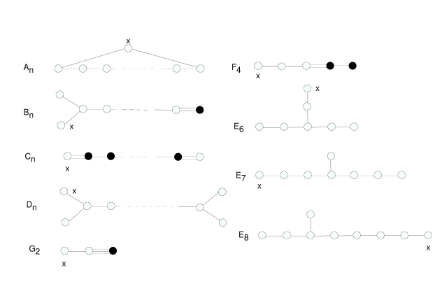
Figure 1: Extended Dynkin diagrams for simple groups. The ordinary Dynkin diagrams are obtained by removing the roots labelled $x$.

Semi-simple maximal regular subgroups can be read off from the Dynkin diagrams obtained by deleting a vertex from the so-called extended Dynkin diagram of a group (fig 1). The final number of vertices is the same as in the original Dynkin diagram, which means that the rank is preserved. The only cases which lead to simple subgroups are

$$\begin{array}[]{ccccc}&SO(2n)&\subset&SO(2n+1)&R_{M}={\bf(2n+1)}\\ &SU(3)&\subset&G_{2}&R_{M}={\bf 7}\\ \tilde{R}_{M}={\bf 9}&SO(9)&\subset&F_{4}&R_{M}={\bf 26}\\ \ast&SU(8)&\subset&E_{7}&\ast\\ \ast&SO(16)&\subset&E_{8}&\ast\\ \ast&SU(9)&\subset&E_{8}&\ast\end{array}\quad.$$ (12)

All these examples have Dynkin index $I_{\tilde{G}\subset G}=1$. We have written down the matter representations in terms of their dimensions, but the examples marked by asterisks unfortunately do not possess suitable matter representations.

One can also delete one of the vertices from the original Dynkin diagram. If it is only connected to one other vertex, the result will be a connected Dynkin diagram, corresponding to a simple subgroup, which is a maximal simple subgroup if the diagram is not a sub-diagram of a simple subgroup obtained from the extended Dynkin diagram. In this way one gets regular subgroups with rank reduced by one. The corresponding sub-theories are obtained by considering only points in the moduli space satisfying ${\bf b\cdot\Lambda}_{k}=0$, where ${\bf\Lambda}_{k}$ is the highest weight of the basic representation corresponding to the deleted vertex. (${\bf\Lambda}_{k}$ is orthogonal to all remaining roots, so in effect we get an orthogonal projection on the space spanned by these roots.) Note the difference of this exact way of finding subgroups, which only works in special cases, and the general but approximate subgroups one finds in the semi-classical regime by strong Higgs breaking [2, 5]. The exact embeddings of theories we find are listed below, together with candidate subgroups which lack appropriate matter representations (marked with asterisks).

$$\begin{array}[]{ccccc}&SU(n-1)&\subset&SU(n)&R_{M}={\bf n}+{\bf\bar{n}}\\ &SO(2n-1)&\subset&SO(2n+1)&R_{M}=2\cdot{\bf(2n+1)}\\ &Sp(2n-2)&\subset&Sp(2n)&R_{M}=2\cdot{\bf(2n)}\\ &SO(2n-2)&\subset&SO(2n)&R_{M}=2\cdot{\bf(2n)}\\ \tilde{R}_{M}=2\cdot{\bf 10}&SO(10)&\subset&E_{6}&R_{M}={\bf 27}+{\bf\bar{27}}\\ &E_{6}&\subset&E_{7}&R_{M}={\bf 56}\\ &SU(2)&\subset&G_{2}&R_{M}=2\cdot{\bf 7}\\ \ast&SU(n)&\subset&SO(2n)&\ast\\ &SU(4)&\subset&SO(8)&R_{M}=2\cdot{\bf 8}_{s}\\ \tilde{R}_{M}={\bf 5}+{\bf\bar{5}}&SU(5)&\subset&SO(10)&R_{M}={\bf 16}+{\bf\bar{16}}\\ &SU(6)&\subset&SO(12)&R_{M}={\bf 32}^{\prime}\\ \ast&SU(n)&\subset&Sp(2n)&\ast\\ &SU(2)&\subset&Sp(4)&R_{M}=2\cdot{\bf 5}\\ &SU(3)&\subset&Sp(6)&R_{M}={\bf 14}^{\prime}\\ \ast&SU(6)&\subset&E_{6}&\ast\\ \ast&SO(12)&\subset&E_{7}&\ast\\ \ast&E_{7}&\subset&E_{8}&\ast\\ \ast&Sp(6)&\subset&F_{4}&\ast\end{array}$$ (13)

These examples also have $I_{\tilde{G}\subset G}=1$. The series of unitary subgroups of orthogonal and symplectic groups, do not in general have matter representations giving asymptotically free theories. Only the special cases that are listed without asterisks satisfy this requirement. If there are several representations of the same dimension, we have distinguished them by the notation of [16].

The special subgroups have been classified by Dynkin [15]. Of the simple subgroups we again list those which are maximal and have unit Dynkin index (an effective criterion to rule out possibilities in this case). Again, embeddings which work are marked by their matter content, and those which do not have appropriate representations are marked by asterisks.

$$\begin{array}[]{ccccc}&SO(2n-1)&\subset&SO(2n)&R_{M}={\bf 2n}\\ &Sp(2n)&\subset&SU(2n)&R_{M}={\bf(n+1)(2n+1)}\\ &G_{2}&\subset&SO(7)&R_{M}={\bf 7}{\rm\ or\ }{\bf 8}\\ &F_{4}&\subset&E_{6}&{\bf 27}\\ \ast&G_{2}&\subset&F_{4}&\ast\\ \ast&G_{2}&\subset&E_{6}&\ast\\ \ast&G_{2}&\subset&E_{7}&\ast\\ \ast&G_{2}&\subset&E_{8}&\ast\\ \ast&Sp(8)&\subset&E_{6}&\ast\\ \ast&Sp(6)&\subset&E_{7}&\ast\\ \ast&F_{4}&\subset&E_{7}&\ast\\ \ast&F_{4}&\subset&E_{8}&\ast\end{array}$$ (14)

To these special group embeddings correspond embeddings of moduli spaces, just as in the case of the regular embeddings. However, we cannot give a simple and general description of the special embeddings.

3 Some regular examples

3.1 $F_{4}$ with fundamental matter

The first of the examples that we will study involves the exceptional group $F_{4}$. The adjoint representation of $F_{4}$ has dimension 52. It has 4 Cartan elements and 48 roots. Let us add one hypermultiplet in the fundamental $\bf{26}$. This will effectively cancel all the long roots leaving only the short ones. The remaining weights are the roots of $SO(8)$. What we actually have used is the regular embedding of $SO(9)$ in $F_{4}$ and the regular embedding of $SO(8)$ in $SO(9)$. Hence we can argue that the low energy theory of $F_{4}$ with one fundamental matter hypermultiplet is the same as the pure $SO(8)$ theory. The check of the Dynkin indices works out as $18-6=12$.

Let us repeat the logic of the argument. Let us assume the existence of the $F_{4}$ solution. The discussion above then shows that this solution obeys all the requirements also of the $SO(8)$ theory (these are less restrictive since the Weyl group is smaller). Hence it follows, if the $SO(8)$ solution is unique, that the $F_{4}$ solution must be identical to the $SO(8)$ solution that we already know. In fact, the existence of the $F_{4}$ theory implies certain symmetries of the $SO(8)$ theory that from the $SO(8)$ point of view look accidental.

There is something surprising about this equivalence. So far all constructions of curves for gauge groups with various types of matter have been invariant under the Weyl group. Indeed, this can be used as an important guide when finding the curves. More precisely, the weight diagram for the fundamental representation of the group has been used to construct the curve. This is the simplest way of finding a representation of the Weyl group. The Weyl group of $F_{4}$ does not leave the suggested curve invariant. However, there is still a way out. The only thing we really need is that the Weyl group is represented on the integrals over the cycles. This is trivially true at the perturbative level, but a very strong requirement non-perturbatively. The reason that this works is the triality symmetry of $SO(8)$. The $SO(8)$ curve is based on the fundamental $\bf{8}$ of $SO(8)$. There are in fact three equivalent representations and therefore three equivalent curves. The $F_{4}$ Weyl elements not contained in the $SO(8)$ Weyl group permute these three different curves. If we set the projections of the weights $(1000)$, $(-1100)$, $(0-111)$ and $(00-11)$ equal to $b_{1}$, $b_{2}$, $b_{3}$ and $b_{4}$ respectively, there is a sequence of $F_{4}$ Weyl transformations that takes

$$b_{1}\rightarrow b_{1}-\Delta_{1}\rightarrow b_{1}-\Delta_{1}-\Delta_{2}\rightarrow b_{1}$$

$$b_{2}\rightarrow b_{2}+\Delta_{1}\rightarrow b_{2}+\Delta_{1}+\Delta_{2}\rightarrow b_{2}$$

$$b_{3}\rightarrow b_{3}+\Delta_{1}\rightarrow b_{3}+\Delta_{1}+\Delta_{2}\rightarrow b_{3}$$

$$b_{4}\rightarrow b_{4}+\Delta_{1}\rightarrow b_{4}+\Delta_{1}-\Delta_{2}\rightarrow-b_{4}$$ (15)

where

$$\Delta_{1}={1\over 2}(b_{1}-b_{2}-b_{3}-b_{4})\;\;\mbox{and}\;\;\Delta_{2}=b_{4}.$$ (16)

This is illustrated in fig. 2. For consistency we must have $a_{1}^{\prime}={1\over 2}(a_{1}+a_{2}+a_{3}+a_{4})$ including the non-perturbative corrections, e.g.,

$$\oint_{\gamma_{1}^{\prime}}\lambda={1\over 2}(\oint_{\gamma_{1}}\lambda+\oint_{\gamma_{2}}\lambda+\oint_{\gamma_{3}}\lambda+\oint_{\gamma_{4}}\lambda),$$ (17)

where the respective cycles are indicated in fig. 2. We have that $\lambda=(2p-xp^{\prime}){dx\over y}$ with $y^{2}=p^{2}-x^{4}\Lambda^{12}$ and $p=(x^{2}-b_{1}^{2})...(x^{2}-b_{4}^{2})$. These integrals are easily calculated in an expansion in $\Lambda^{12}$. It can be checked that (17) is really satisfied.

Figure 2: The three curves for $F_{4}$ with fundamental matter interchanged by $SO(8)$ triality.

From this we can conclude that $F_{4}$ with one massless fundamental hypermultiplet is given by

$$y^{2}=((x^{2}-b_{1}^{2})(x^{2}-b_{2}^{2})(x^{2}-b_{3}^{2})(x^{2}-b_{4}^{2}))^{2}-x^{4}\Lambda^{12}$$ (18)

We emphasize again that the curve can not be written in terms of the $F_{4}$ Casimirs.

3.2 $G_{2}$ with fundamental matter

There is an even simpler example of the phenomena discussed above. Let us consider $G_{2}$ with matter in the fundamental $\bf{7}$. The effective low energy theory can be shown to be the same as that of pure $SU(3)$. The breaking to $SU(3)$ gives ${\bf 14}\rightarrow{\bf 8}+{\bf 3}+\bar{\bf 3}$ for the adjoint and ${\bf 7}\rightarrow{\bf 1}+{\bf 3}+\bar{\bf 3}$ for the fundamental. The fundamental ${\bf 3}$ and $\bar{\bf 3}$ hypermultiplets cancel the corresponding vector multiplets and leave a pure $SU(3)$ theory. Again we have the problem that the curve is not Weyl invariant. The $SU(3)$ curve is based on the fundamental ${\bf 3}$ of $SU(3)$. Under the $G_{2}$ Weyl group the ${\bf 3}$ is transformed into the $\bar{\bf 3}$. In fact, the $SU(3)$ curve is simply reflected through the origin.

3.3 $E_{6}$ with two fundamentals

Finally we give some results for the group $E_{6}$. There is a regular embedding of $SO(10)$ in $E_{6}$. In fact, the adjoint of $E_{6}$ breaks like ${\bf 78}\rightarrow{\bf 45}+{\bf 16}+\bar{\bf 16}+\bf{1}$. If we add a fundamental and an anti-fundamental hypermultiplet to the $E_{6}$ theory which break like ${\bf 27}\rightarrow{\bf 16}+{\bf 10}+\bf{1}$ (and the corresponding pattern for the anti-fundamental), we obtain $SO(10)$ with two fundamental hypermultiplets. The check of Dynkin indices also works out: $24-2\times 6=16-2\times 2$. Unfortunately the proposed curve can only describe a codimension 1 subspace of the $E_{6}$ moduli space.

We might note that the $F_{4}$ curve above also describes parts of the $E_{6}$ moduli space, since there is a special embedding of $F_{4}$ in $E_{6}$. In that case only a codimension 2 subspace is accessible.

4 Some special examples

4.1 $SO(6)\rightarrow SO(5)$

The adjoint representation of $SO(6)$ has dimension 15. The weights of the adjoint correspond to the 3 Cartan elements and the 12 roots. The weight diagram, with weights labelled by their Dynkin labels, see e.g. [17], is given in fig 3.

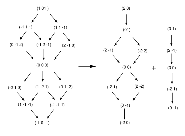
Figure 3: The breaking $\bf{15}\rightarrow\bf{10}+\bf{5}$ of $SU(4)$ to $SO(5)$.

The $(mass)^{2}$ of the gauge bosons are then proportional to $(\mbox{\boldmath$\alpha$}\cdot{\bf b})^{2}$. Let us now finetune the Higgs expectation value by setting $b_{1}=b_{3}$. We furthermore introduce $\tilde{b}_{1}={b_{1}+b_{3}\over 2}$ and $\tilde{b}_{2}=b_{2}$. A new, reduced weight diagram can now be constructed through $\mbox{\boldmath$\alpha$}\cdot{\bf b}\rightarrow{\bf w}\cdot\tilde{\bf b}$. It is drawn on the right of fig. 3 where one can identify the $\bf 10$ (adjoint) and $\bf 5$ (fundamental) of $SO(5)$. From the $SO(5)$ point of view we have vector-multiplets both in the adjoint and the fundamental of $SO(5)$. Clearly this theory only makes sense thanks to the embedding in $SO(6)$.

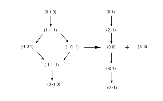
Figure 4: The breaking $\bf{6}\rightarrow\bf{5}+\bf{1}$ of $SU(4)$ to $SO(5)$.

Let us now add matter in the $\bf 6$ to the $SO(6)$ theory. We can also think of this as an $SU(4)$ theory where we add matter in a tensor representation. The $\bf 6$ breaks to a $\bf{5}+\bf{1}$ according to fig. 4. The hypermultiplet will have charges and hence masses identical to the vector multiplet in the fundamental representation. It follows then from (4) that the fundamental hypermultiplet will cancel the contribution of the fundamental vector multiplet and leave a pure $SO(5)$ theory. We should also check that the Dynkin indices come out correctly. For $SO(6)$ we have $8-2=6$ which agrees with pure $SO(5)$.

4.2 Pure $G_{2}$

Let us now use the above ideas to work out the details for an exceptional example, $G_{2}$. The adjoint, i.e. the $\bf 21$, of $SO(7)$ breaks to $\bf{14}+\bf{7}$ of $G_{2}$. In the same way, the fundamental $\bf 7$ of $SO(7)$ goes to the fundamental $\bf 7$ of $G_{2}$. This means that the contribution of the extra vector multiplets in the $G_{2}$ picture can be cancelled by adding a hypermultiplet in the fundamental representation of $G_{2}$. We therefore conclude that the pure $G_{2}$ theory can be obtained by restricting the Higgs expectation values of an $SO(7)$ theory with a fundamental hypermultiplet. This is also the same as a pure $SO(6)$ theory. The Dynkin indices work out as $10-2=8$.

Let us check this in more detail! In fig. 5 we have drawn a choice of cycles for $SO(7)$.

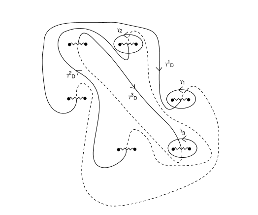
Figure 5: Cycles for $SO(7)$ to be used for $G_{2}$.

The action of the three simple monodromies are shown in fig. 6. The corresponding monodromy matrices are (in orthogonal basis)

$$M_{1}=\pmatrix{0&1&0&1&-1&0\cr 1&0&0&-1&1&0\cr 0&0&1&0&0&0\cr 0&0&0&0&1&0\cr 0&0&0&1&0&0\cr 0&0&0&0&0&1\cr}\;\;,\;\;M_{2}=\pmatrix{1&0&0&0&0&0\cr 0&0&1&0&1&-1\cr 0&1&0&0&-1&1\cr 0&0&0&1&0&0\cr 0&0&0&0&0&1\cr 0&0&0&0&1&0\cr},$$

$$M_{3}=\pmatrix{1&0&0&0&0&0\cr 0&1&0&0&0&0\cr 0&0&-1&0&0&0\cr 0&0&0&1&0&0\cr 0&0&0&0&1&0\cr 0&0&0&0&0&-1\cr}\hskip 85.35826pt$$ (19)

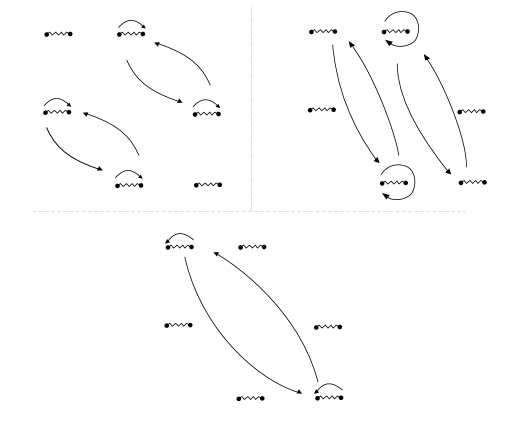
Figure 6: Simple monodromies for $SO(7)$ with matter to be combined as $G_{2}$ monodromies.

To break to $G_{2}$ we must make a finetuning of the Higgs expectation values so that we can write

$$b_{1}=\tilde{b}_{2}\;\;,b_{2}=\tilde{b}_{1}-\tilde{b}_{2},\;\;\mbox{and}\;\;b_{3}=2\tilde{b}_{2}-\tilde{b}_{1},$$ (20)

where $\tilde{b}_{i}$ are the Higgs expectation values in the $G_{2}$ theory. The magnetic masses of the $G_{2}$ theory will be given by

$$a_{1}^{D}={1\over 2}({i\over 2\pi}\oint_{\gamma_{2}^{D}}\lambda-{i\over 2\pi}\oint_{\gamma_{3}^{D}}\lambda)$$

$$a_{2}^{D}={1\over 2}({i\over 2\pi}\oint_{\gamma_{1}^{D}}\lambda-{i\over 2\pi}\oint_{\gamma_{2}^{D}}\lambda)+{i\over 2\pi}\oint_{\gamma_{3}^{D}}\lambda.$$ (21)

The expressions for the magnetic cycles follow from $a_{i}^{D}=\frac{\partial{\cal F}}{\partial a_{i}}$. We have chosen Dynkin basis for the $G_{2}$ group. With these definitions we can write down the two simple monodromies of $G_{2}$ as

$$M_{1}M_{3}=\pmatrix{1&1&-1&2\cr 0&-1&2&-4\cr 0&0&1&0\cr 0&0&1&-1\cr}, M_{2}=\pmatrix{-1&0&-4&6\cr 3&1&6&-9\cr 0&0&-1&3\cr 0&0&0&1\cr},$$ (22)

which is precisely what to be expected. We recall the general formula obtained in [5];

$$M_{k}\equiv\pmatrix{W^{t}&-\mbox{\boldmath$\alpha$}_{k}\otimes\mbox{\boldmath$\alpha$}_{k}\cr 0&W\cr}.$$ (23)

We conclude that the pure $G_{2}$ theory is described by

$$y^{2}=((x^{2}-b_{1}^{2})(x^{2}-b_{2}^{2})(x^{2}-b_{3}^{2}))^{2}-x^{4}\Lambda^{8}.$$ (24)

where $b_{1}$, $b_{2}$ and $b_{3}$ are given by (20). One can note that the curve is based on the fundamental weight diagram of $G_{2}$.

5 An odd example

Let us end with an equivalence that does not comfortably fit in the two classes discussed above. This illustrates that maps between weght diagrams are the primary objects in the equivalences, and subgroups just give a natural way to generate these maps. We will consider $SU(4)\rightarrow SO(5)$, where we add two hypermultiplets in the $\bf{4}$ to the $SU(4)$ theory. Under the above breaking the $\bf{4}$ breaks like in fig. 7.

Figure 7: The breaking $\bf{4}\rightarrow\bf{4}$ of $SU(4)$ to $SO(5)$ (or $Sp(4)$).

Let us add these contributions to the broken adjoint of fig. 3 and write down the prepotential. It is given by

$${\cal F}\sim{i\over 4\pi}\bigg{(}2({\bf b}\cdot\mbox{\boldmath$\alpha$}_{1})^{2}\log{({\bf b}\cdot\mbox{\boldmath$\alpha$}_{1})^{2}\over\Lambda^{2}}+({\bf b}\cdot\mbox{\boldmath$\alpha$}_{2})^{2}\log{({\bf b}\cdot\mbox{\boldmath$\alpha$}_{2})^{2}\over\Lambda^{2}}$$

$$+2({\bf b}\cdot(\mbox{\boldmath$\alpha$}_{1}+\mbox{\boldmath$\alpha$}_{2}))^{2}\log{({\bf b}\cdot(\mbox{\boldmath$\alpha$}_{1}+\mbox{\boldmath$\alpha$}_{2}))^{2}\over\Lambda^{2}}+({\bf b}\cdot(2\mbox{\boldmath$\alpha$}_{1}+\mbox{\boldmath$\alpha$}_{2}))^{2}\log{({\bf b}\cdot(2\mbox{\boldmath$\alpha$}_{1}+\mbox{\boldmath$\alpha$}_{2}))^{2}\over\Lambda^{2}}$$

$$-2({\bf b}\cdot\mbox{\boldmath$\alpha$}_{2}/2)^{2}\log{({\bf b}\cdot\mbox{\boldmath$\alpha$}_{2}/2)^{2}\over\Lambda^{2}}-2({\bf b}\cdot(2\mbox{\boldmath$\alpha$}_{1}+\mbox{\boldmath$\alpha$}_{2})/2)^{2}\log{({\bf b}\cdot(2\mbox{\boldmath$\alpha$}_{1}+\mbox{\boldmath$\alpha$}_{2})/2)^{2}\over\Lambda^{2}}\bigg{)}.$$ (25)

The factor $2$ in the first and third term is due to the extra vector multiplets we discussed in the previous subsection, the factor $2$ in the last two terms is present since there are two hypermultiplets. Note also the factor $1/2$ in the charge of the hypermultiplets. One can easily check that the prepotential of $SO(5)$ is obtained after a renaming of the long and short roots, i.e. $\mbox{\boldmath$\alpha$}_{2}\rightarrow\sqrt{2}\mbox{\boldmath$\alpha$}_{1}$ and $\mbox{\boldmath$\alpha$}_{1}\rightarrow{1\over\sqrt{2}}\mbox{\boldmath$\alpha$}_{2}$. This indeed results in the prepotential of pure $SO(5)$. The check of Dynkin indices again works out: $8-2\times 1=6$. The curves, according to equations (5) and (7) are identical.

6 Conclusions

In this paper we have described some equivalences between different $N=2$ supersymmetric Yang-Mills theories. We have found all equivalences based on maximal simple subgroups of simple Lie groups, and we have also observed in an example that more general constructions are possible. We have used these equivalences to construct solutions of some theories with exceptional gauge groups. It is interesting to note that in some cases we need to relax the requirement of Weyl invariance of the complex curves. In effect, part of the large Weyl symmetry in these theories is hidden. This allows hyperelliptic curves to describe a larger set of theories. It is our hope that these ideas can be of help also in a more general context.

References

- [1] N. Seiberg and E. Witten, Nucl. Phys. B426 (1994) 19, B431 (1994) 484.
- [2] P.C. Argyres and A.E. Faraggi, Phys. Rev. Lett. 74 (1995) 3931, hep-th/9411057.
- [3] A. Klemm, W. Lerche, S. Yankielowicz and S. Theisen, Phys. Lett. 344B (1995) 169, hep-th/9411048; CERN-TH.7538/94, LMU-TPW 94-22, hep-th/9412158; CERN-TH. 95-104, LMU-TPW 95-7, hep-th/9505150.
- [4] M.R. Douglas and S.H. Shenker, Nucl. Phys. B447 (1995) 271, hep-th/9503163.
- [5] U. H. Danielsson and B. Sundborg, Phys. Lett. B358 (1995) 273, hep-th/9504102.
- [6] P.C. Argyres, M.R. Plesser and A.D. Shapere, Phys. Rev. Lett. 75 (1995) 1699, hep-th/9505075.
- [7] A. Hanany and Y. Oz, Nucl. Phys. B452 (1995) 283, hep-th/9505075.
- [8] A. Brandhuber and K. Landsteiner, Phys. Lett. 358 (1995) 73, hep-th/9507008.
- [9] J.A. Minahan and D. Nemeschansky, ‘Hyperelliptic Curves for Supersymmteric Yang-Mills’, CERN-TH. 95-167, hep-th/9507032.
- [10] P.C. Argyres and A.D. Shapere, ‘The Vacuum Structure of Super-QCD with Classical Gauge Groups’, RU-95-61, UK/95-14, hep-th/9509175.
- [11] A. Hanany, ‘On the Quantum Moduli Space of Vacua of Supersymmetric Gauge Theories’, IASSNS-HEP-95/76, hep-th/9509176.
- [12] R. Donagi and E. Witten, “Supersymmetric Yang-Mills Theory and Integrable Systems”, IASSNS-HEP-95-78, hep-th/9510101.
- [13] E. Martinec and N. Warner, “Integrable Systems and Supersymmetric Yang-Mills Theory”, EFI-95-61, USC-95/025, hep-th/9509162.
- [14] B. de Wit, P. Lauwers and A. Van Proyen, Nucl. Phys. B255 (1985) 269.
- [15] E.B. Dynkin, Amer. Math. Soc. Transl. Ser. 2,6 (1957) 111 and 245.
- [16] R. Slansky, Phys. Rep. vol 79, no 1, 1981.
- [17] J. Fuchs, “Affine Lie Algebras and Quantum Groups”, Cambridge University Press 1992.