Operator Product Expansion

in Two-Dimensional Quantum Gravity

Hajime Aoki¹⁾, Hikaru Kawai¹⁾, Jun Nishimura²⁾and Asato Tsuchiya^1)
1) National Laboratory for High Energy Physics (KEK),
Tsukuba, Ibaraki 305, Japan

²⁾ Department of Physics, Nagoya University ,

Chikusa-ku, Nagoya 464-01, Japan

We consider correlation functions of operators and the operator product expansion in two-dimensional quantum gravity. First we introduce correlation functions with geodesic distances between operators kept fixed. Next by making two of the operators closer, we examine if there exists an analog of the operator product expansion in ordinary field theories. Our results suggest that the operator product expansion holds in quantum gravity as well, though special care should be taken regarding the physical meaning of fixing geodesic distances on a fluctuating geometry.

1 Introduction

There has been considerable success in the study of quantum gravity within the framework of field theory in recent years. Particularly, in two dimensions, a continuum formalism (Liouville theory) as well as a discretized formalism (dynamical triangulation) has been consistently developed, and they are shown to give equivalent results [1]. Correlation functions have been obtained analytically and they are found to satisfy closed recursive relations, which make the theory solvable [2]. In spite of these developments, we are still lacking in the viewpoints of the renormalization group and the operator product expansion (OPE), which would provide a way to see how the theory behaves when we change the scale. The main difficulty in their realization lies in the fact that in quantum gravity the metric field, which could be used to fix the scale, is integrated over.

There have been several attempts to study the renormalization group in quantum gravity. In $2+\epsilon$-dimensional quantum gravity, the renormalization point can be introduced as in the ordinary perturbation theory, and the dependence of the coupling constants on the renormalization point has been studied [3]. Block-spin transformation has been considered in the context of dynamical triangulation by various people, and numerical studies seem to support the validity of the formalism at least in two dimensions [4]. Also there is a study on the effects of the gravitational dressing to the renormalization group in two-dimensional quantum gravity [5].

However, the OPE in quantum gravity has not been studied yet. In this paper, we study it in two-dimensional quantum gravity. For this purpose, we must introduce the notion of the distance between local operators. In quantum gravity we can use the geodesic distance, which is general coordinate invariant. Recently a formalism has been developed, which enables us to introduce the geodesic distance [6, 7]. Using this formalism we calculate correlation functions with fixed geodesic distances between the operators. By making two of the operators closer to each other, we examine if there exist OPE like relations among the operators. We insert other operators as observers and compare the correlation functions. However, since the metric is fluctuating in quantum gravity, it is not trivial if fixing the geodesic distance corresponds exactly to fixing the scale as in the ordinary quantum field theory in the flat space. The OPE is expected to hold as a result of integrating out the local degrees of freedom. In quantum gravity, however, the meaning of the local degrees of freedom is somewhat obscure, since the metric itself is the dynamical variable. The observers, each of which we require to be at a definite distance from the two close operators, might be sensitive to some large fluctuations of “the local degrees of freedom” which should have been integrated out. We would like to shed light on such a subtlety in fixing geodesic distance in quantum gravity.

Another interesting aspect we can elucidate by using this kind of correlation functions is the fractal structure of the space-time, which has been revealed in two dimensions in Ref. [6]. There, sections of the two-dimensional surface were considered, each of which was at a fixed geodesic distance from a given point. A typical section is composed of loops of various lengths, whose distribution could be calculated analytically. The loop-length distribution shows a scaling behavior, which can be interpreted as the fractal structure of space-time. However, it was found that the total length of the section at a fixed geodesic distance is divergent, and in this sense the fractal structure can only be seen in a somewhat indirect way through the loop-length distribution. Here we show that the two-point functions of the cosmological constant terms with fixed geodesic distances provides a more direct way to see the fractal structure.

This paper is organized as follows. In Section 2, we introduce two-point functions with fixed geodesic distances. In Section 3, we show how we can see the fractal structure of the space-time in a direct way using these two-point functions. In Section 4, we calculate three-point functions with fixed geodesic distances. By using them, together with the results for one-point and two-point functions, we examine whether there are OPE like operator relations or not. Section 5 is devoted to the summary and outlook.

2 Two-point Functions with Fixed Geodesic Distances

Throughout this paper, we consider pure gravity in two dimensions. For simplicity, the topology of the two-dimensional manifold is restricted to be a sphere. We introduce a correlation function of two loops with fixed geodesic distance, which is formally defined as follows (See Fig. 1).

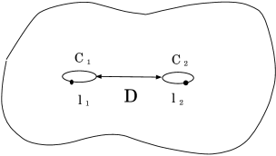
Figure 1: The correlation function of two loops with fixed geodesic distance $D$. The geodesic distance between the loop $C_{1}$ of length $l_{1}$ and the loop $C_{2}$ of length $l_{2}$ is fixed to be $D$. Each of the loops is considered to have a marking point.

$$G(l_{1},l_{2};D;t) = \int\frac{{\cal D}g}{\mbox{Vol(Diff)}}~{}\delta(\int_{C_{1}}\sqrt{g_{\mu\nu}\mbox{d}x^{\mu}\mbox{d}x^{\nu}}-l_{1})~{}\delta(\int_{C_{2}}\sqrt{g_{\mu\nu}\mbox{d}x^{\mu}\mbox{d}x^{\nu}}-l_{2})$$ (2.1)

$$\delta(d(C_{1},C_{2})-D)~{}\mbox{e}^{-t\int\mbox{\scriptsize d}^{2}x\sqrt{g}}.$$

The geodesic distance $d(C_{1},C_{2})$ between the loops $C_{1}$ and $C_{2}$ is defined by

$$d(C_{1},C_{2})=\min_{P_{1}\in C_{1},P_{2}\in C_{2}}d(P_{1},P_{2}),$$ (2.2)

where $d(P_{1},P_{2})$ is the geodesic distance between the points $P_{1}$ and $P_{2}$ in the ordinary sense. Here we consider such an amplitude that each of the loops $C_{1}$ and $C_{2}$ has a marking point.

This quantity can be calculated using the proper-time evolution kernel, which is defined as the amplitude with the entrance loop $C$ of length $l$ and the exit loop of length $l^{\prime}$, where each point $P^{\prime}$ on the exit loop $C^{\prime}$ is at the geodesic distance $D$ from the entrance loop $C$ in the sense that

$$\min_{P\in C}d(P^{\prime},P)=D.$$ (2.3)

We adopt the convention that the exit loop has a marking point and the entrance loop not. The Laplace transform of the proper-time evolution kernel is obtained as [6]

$$N(\zeta,\zeta^{\prime};D;t)=\frac{1}{\zeta^{\prime}+A(\zeta;D;t)}.$$ (2.4)

$A(\zeta;D;t)$ is a function defined as

$$A(\zeta;D;t)=f(xf^{-1}(\zeta)),$$ (2.5)

where

$$x = \mbox{e}^{\sqrt{6}~{}t^{1/4}D},$$ (2.6)

$$f(y) = \sqrt{t}~{}\left\{\frac{3}{2}\left(\frac{2}{y-1}+1\right)^{2}-1\right\},$$ (2.7)

$$f^{-1}(\zeta) = \frac{\sqrt{6}~{}t^{1/4}}{\sqrt{\zeta+\sqrt{t}}-\sqrt{\frac{3}{2}}~{}t^{1/4}}+1.$$ (2.8)

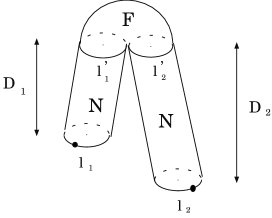
Figure 2: Calculation of the correlation function of two loops $G(l_{1},l_{2};D;t)$. The diagram corresponds to Eq. (2.9). The correlation function of two loops can thus be calculated using the disk amplitude $F$ and the proper-time evolution kernel $N$.

Using the proper-time evolution kernel, we can express the correlation function of two loops $G(l_{1},l_{2};D;t)$ as

$$G(l_{1},l_{2};D;t)=l_{1}~{}l_{2}~{}\int_{0}^{\infty}\mbox{d}l_{1}^{\prime}\int_{0}^{\infty}\mbox{d}l_{2}^{\prime}~{}F(l_{1}^{\prime}+l_{2}^{\prime};t)~{}N(l_{1},l_{1}^{\prime};D_{1};t)~{}N(l_{2},l_{2}^{\prime};D_{2};t),$$ (2.9)

where $F(l;t)$ is the disc amplitude, whose Laplace transform is given by

$$F(\zeta;t)=(2\zeta-\sqrt{t})\sqrt{\zeta+\sqrt{t}},$$ (2.10)

and $D=D_{1}+D_{2}$. Fig. 2 indicates the diagram corresponding to Eq. (2.9). Eq. (2.9) can be evaluated as

$$G(\zeta_{1},\zeta_{2};D;t) = \frac{\partial}{\partial\zeta_{1}}~{}\frac{\partial}{\partial\zeta_{2}}~{}\int\frac{\mbox{d}\zeta}{2\pi i}~{}F(\zeta;t)~{}N(\zeta_{1},-\zeta;D_{1};t)~{}N(\zeta_{2},-\zeta;D_{2};t)$$ (2.11)

$$= -\frac{\partial}{\partial\zeta_{1}}~{}\frac{\partial}{\partial\zeta_{2}}~{}\frac{F(A_{1})-F(A_{2})}{A_{1}-A_{2}}$$ (2.12)

$$= -2\sqrt{6}~{}t^{1/4}\frac{1+y_{1}y_{2}}{(1-y_{1}y_{2})^{3}}\frac{\partial y_{1}}{\partial\zeta_{1}}\frac{\partial y_{2}}{\partial\zeta_{2}},$$ (2.13)

where

$$A_{i} = A(\zeta_{i};D_{i};t),$$ (2.14)

$$y_{i} = x_{i}f^{-1}(\zeta_{i}),$$ (2.15)

$$x_{i} = \mbox{e}^{\sqrt{6}~{}t^{1/4}D_{i}}.$$ (2.16)

The r.h.s of (2.13) should depend only on $D=D_{1}+D_{2}$, and this is indeed the case since it is written in terms of $y_{1}y_{2}$, which is

$$y_{1}y_{2} = x_{1}x_{2}f^{-1}(\zeta_{1})f^{-1}(\zeta_{2})$$ (2.17)

$$= \mbox{e}^{\sqrt{6}~{}t^{1/4}(D_{1}+D_{2})}f^{-1}(\zeta_{1})f^{-1}(\zeta_{2}).$$ (2.18)

This is an example of the consistency condition mentioned in Ref. [8].

Let us next pinch the loops in order to obtain the local operators. This can be done by expanding the above result in terms of $1/\sqrt{\zeta_{1}}$ and $1/\sqrt{\zeta_{2}}$ as

$$G(\zeta_{1},\zeta_{2};D;t)=\sum_{n,m=1}^{\infty}G_{nm}(D,t)~{}\zeta_{1}^{-(\frac{n}{2}+1)}\zeta_{2}^{-(\frac{m}{2}+1)},$$ (2.19)

where $G_{nm}(D,t)$ can be regarded as the two-point correlation function of the operators ${\cal O}_{n}$ and ${\cal O}_{m}$ with the fixed geodesic distance $D$.

$$G_{nm}(D;t)=\langle{\cal O}_{n}{\cal O}_{m}(D)\rangle.$$ (2.20)

The explicit forms of $G_{nm}$’s are obtained as

$$G_{11}(D,t) = 3\sqrt{6}~{}t^{3/4}~{}\frac{(x+1)~{}x}{(x-1)^{3}},$$

$$G_{12}(D,t) = -18~{}t~{}\frac{(x^{2}+4x+1)~{}x}{(x-1)^{4}},$$

$$G_{22}(D,t) = 18\sqrt{6}~{}t^{5/4}~{}\frac{(x+1)(x^{2}+10x+1)~{}x}{(x-1)^{5}},$$

$$\vdots$$

where $x=\mbox{e}^{\sqrt{6}~{}t^{1/4}D}$. Note that when one considers correlation functions of loops without fixing the geodesic distances and expands them in terms of $1/\sqrt{\zeta_{i}}$, one encounters only odd powers in contrast to the above results where we encounter even powers as well. If we integrate $G_{nm}(D,t)$ over $D$ from 0 to the infinity, we reproduce the conventional results of the two-point functions. Indeed the cases including at least one even number index vanish after the integration. This means that we have found a new set of operators ${\cal O}_{n}$ with even $n$, which cannot be seen without fixing the geodesic distance. We also comment that $G_{11}(D,t)$ agrees with the result obtained in Ref. [9] in a different way.

3 Fractal Structure of the Space-time

Using the two-point correlation functions with fixed geodesic distances obtained in the previous section, we can study the fractal structure of the space-time. For this purpose, let us consider the two-point correlation function of the cosmological constant terms, which can be formally written in the following way.

$$V^{\prime}(D)=\lim_{A\rightarrow\infty}\frac{1}{A}\frac{\int\frac{{\cal D}g}{\mbox{\scriptsize Vol(Diff)}}~{}\int\mbox{d}^{2}x_{1}\sqrt{g(x_{1})}~{}\int\mbox{d}^{2}x_{2}\sqrt{g(x_{2})}~{}\delta(d(x_{1},x_{2})-D)~{}\delta(\int\sqrt{g}\mbox{d}^{2}x-A)}{\int\frac{{\cal D}g}{\mbox{\scriptsize Vol(Diff)}}~{}\delta(\int\sqrt{g}\mbox{d}^{2}x-A)}.$$ (3.1)

This quantity can be identified with the $D$-derivative of the volume of the region within the geodesic distance $D$ from a given point. Therefore, if $V^{\prime}(D)$ behaves as $D^{d_{h}-1}$, we can identify $d_{h}$ as the Hausdorff dimension of the space-time.

The thermodynamic limit $A\rightarrow\infty$ can be obtained by expanding Laplace-transformed expressions around $t=0$. If we expand $F(\zeta;t)$ in terms of $t$, we have

$$F(\zeta;t) = \sum_{k\geq-5;\mbox{\scriptsize odd}}F_{k}(t)~{}\zeta^{-(\frac{k}{2}+1)}$$ (3.2)

$$= 2~{}\zeta^{3/2}-\frac{3}{4}~{}\zeta^{1/2}~{}t+\frac{1}{4}~{}\zeta^{-3/2}~{}t^{3/2}+O(t^{2}).$$

Since the first two terms come from small universes, they should be subtracted when we take the thermodynamic limit $t\rightarrow 0$. Therefore the only one-point function that remains nonzero after the thermodynamic limit is $F_{1}$. As in the case of two-point functions, we identify $F_{1}$ as an expectation value of the scaling operator ${\cal O}_{1}$, which is known to correspond to the cosmological constant term. In what follows, we use the notation

$$F_{1}^{\mbox{\scriptsize(T.D.)}} = \frac{1}{4}~{}t^{3/2},$$ (3.3)

$$F_{k}^{\mbox{\scriptsize(T.D.)}} = 0~{}~{}~{}~{}~{}~{}~{}~{}~{}(k\neq 1).$$ (3.4)

Similarly if we expand $G_{11}$ in terms of $t$, we have

$$G_{11}(D;t)=\frac{1}{D^{3}}-\frac{3}{20}~{}D~{}t+\frac{1}{14}~{}D^{3}~{}t^{3/2}+O(t^{2}).$$ (3.5)

Hence in the thermodynamic limit, we have

$$G_{11}^{\mbox{\scriptsize(T.D.)}}(D)=\frac{1}{14}~{}D^{3}~{}t^{3/2}.$$ (3.6)

Here, we have two terms $O(t^{0})$ and $O(t^{1})$ that have to be subtracted when we take the $t\rightarrow 0$ limit, which is in contrast to the case of the usual cylinder amplitude, where we need only one subtraction. This can be naturally understood, since the two operators, which are constrained to be apart from each other by the distance $D$, behave as one operator in a large space-time.

Using the above expressions in the thermodynamic limit, (3.1) can be evaluated as

$$V^{\prime}(D)=\frac{G_{11}^{\mbox{\scriptsize(T.D.)}}}{F_{1}^{\mbox{\scriptsize(T.D.)}}}=\frac{2}{7}~{}D^{3}.$$ (3.7)

Therefore, the Hausdorff dimension of the space-time is $d_{h}=4$, which agrees with the one given through the loop-length distribution [6]. In Ref. [6], it has been pointed out that the total length of the boundary at the geodesic distance $D$ from a given point is not well-defined in the continuum limit. However, the area of the region within the geodesic distance $D\sim D+\Delta D$ is a well-defined quantity as we have seen. Thus, we are able to observe the fractal structure of the space-time more directly by considering the two-point correlation functions of the cosmological constant terms than by considering the loop-length distribution.

We note that in Ref. [9] it is also argued that $d_{h}=4$ by examining the scaling behavior for the finite volume universe.

4 Operator Product Expansion in Quantum Gravity

In this section, we examine if the operator product expansion holds in quantum gravity in the sense that two operators close to each other can be regarded as one when viewed from a distance. Although we are able to obtain some of the OPE coefficients by comparing two-point functions and one-point functions, the first nontrivial check of the OPE as operator relations can be given by inserting one extra operator as an observer. For this purpose, we need the three-point functions, which we calculate in the next subsection.

4.1 Three-Point Functions with Fixed Geodesic Distances

We consider a correlation function of three loops with fixed geodesic distances, which is formally defined as follows (See Fig. 3).

$$H(l_{1},l_{2},l_{3};D;D^{\prime};t) = \int\frac{{\cal D}g}{\mbox{Vol(Diff)}}\prod_{i=1}^{3}~{}\delta(\int_{C_{i}}\sqrt{g_{\mu\nu}\mbox{d}x^{\mu}\mbox{d}x^{\nu}}-l_{i})$$ (4.1)

$$\delta(d(C_{1},C_{2})-D)~{}\delta(d(C_{1}\cup C_{2},C_{3})-D^{\prime})~{}\mbox{e}^{-t\int\mbox{\scriptsize d}^{2}x\sqrt{g}},$$

where we have specified the geodesic distance between $C_{3}$ and the union of $C_{1}$ and $C_{2}$. Each of the three loops is considered to have a marking point.

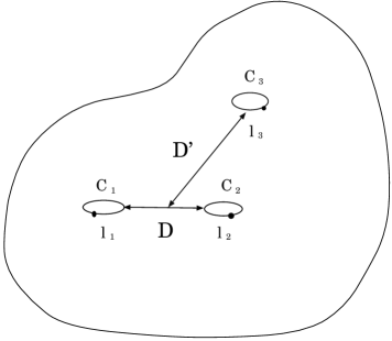
Figure 3: The correlation function of three loops with fixed geodesic distances. The geodesic distance between the loop $C_{1}$ of length $l_{1}$ and the loop $C_{2}$ of length $l_{2}$ is fixed to be $D$. The geodesic distance between the loop $C_{3}$ of length $l_{3}$ and the union of the loops $C_{1}$ and $C_{2}$ is fixed to be $D^{\prime}$. Each of the loops is considered to have a marking point.

When $D<D^{\prime}$, we can calculate the above quantity by the same technique with which we calculate the correlation functions of two loops. $H(l_{1},l_{2},l_{3};D;D^{\prime};t)$ can be calculated as the sum of three contributions.

$$H(l_{1},l_{2},l_{3};D;D^{\prime};t)=H_{\mbox{\scriptsize I}}(l_{1},l_{2},l_{3};D;D^{\prime};t)+H_{\mbox{\scriptsize II}}(l_{1},l_{2},l_{3};D;D^{\prime};t)+H_{\mbox{\scriptsize II}}^{\prime}(l_{1},l_{2},l_{3};D;D^{\prime};t).$$ (4.2)

$H_{\mbox{\scriptsize I}}$ and $H_{\mbox{\scriptsize II}}$ correspond to the two diagrams in the l.h.s. of Fig. 4 respectively. $H_{\mbox{\scriptsize II}}^{\prime}$ can be obtained by exchanging $l_{1}$ and $l_{2}$ in $H_{\mbox{\scriptsize II}}$.

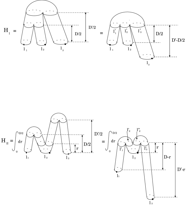
Figure 4: Calculation of the correlation function of three loops $H(l_{1},l_{2},l_{3};D;D^{\prime};t)$. The diagrams in the r.h.s. correspond to Eq. (4.3) and Eq. (4.4) respectively. The equalities of the diagrams come from the consistency condition.

Making use of the consistency condition, we can evaluate $H_{\mbox{\scriptsize I}}$ and $H_{\mbox{\scriptsize II}}$ by the diagrams in the r.h.s. of Fig. 4, which can be expressed as

$$H_{\mbox{\scriptsize I}}(l_{1},l_{2},l_{3};D;D^{\prime};t) = l_{1}~{}l_{2}~{}l_{3}~{}\int_{0}^{\infty}\mbox{d}l_{1}^{\prime}~{}\mbox{d}l_{2}^{\prime}~{}\mbox{d}l_{3}^{\prime}~{}(l_{1}^{\prime}+l_{2}^{\prime})~{}F(l_{1}^{\prime}+l_{2}^{\prime}+l_{3}^{\prime})$$ (4.3)

$$N(l_{1},l_{1}^{\prime};\frac{D}{2};t)~{}N(l_{2},l_{2}^{\prime};\frac{D^{\prime}}{2};t)~{}N(l_{3},l_{3}^{\prime};D^{\prime}-\frac{D}{2};t),$$

$$H_{\mbox{\scriptsize II}}(l_{1},l_{2},l_{3};D;D^{\prime};t) = l_{1}~{}l_{2}~{}l_{3}~{}\int_{0}^{D/2}\mbox{d}r\int_{0}^{\infty}\mbox{d}l_{1}^{\prime}~{}\mbox{d}l_{2}^{\prime}~{}\mbox{d}l_{2}^{\prime\prime}~{}\mbox{d}l_{3}^{\prime}~{}l_{2}^{\prime}~{}l_{2}^{\prime\prime}~{}F(l_{1}^{\prime}+l_{2}^{\prime})~{}F(l_{2}^{\prime\prime}+l_{3}^{\prime})$$ (4.4)

$$N(l_{1},l_{1}^{\prime};D-r;t)~{}N(l_{2},l_{2}^{\prime}+l_{2}^{\prime\prime};r;t)~{}N(l_{3},l_{3}^{\prime};D^{\prime}-r;t).$$

We obtain the following results for $H_{\mbox{\scriptsize I}}$ and $H_{\mbox{\scriptsize II}}$.

$$H_{\mbox{\scriptsize I}}(\zeta_{1},\zeta_{2},\zeta_{3};D;D^{\prime};t)$$ (4.5)

$$= \frac{\partial}{\partial\zeta_{1}}~{}\frac{\partial}{\partial\zeta_{2}}~{}\frac{\partial}{\partial\zeta_{3}}~{}\left[F^{\prime}(A_{1})\frac{1}{A_{1}-A_{2}}\frac{1}{A_{1}-A_{3}}+F^{\prime}(A_{2})\frac{1}{A_{2}-A_{1}}\frac{1}{A_{2}-A_{3}}\right.$$

$$-F(A_{1})\frac{1}{A_{1}-A_{2}}\frac{1}{(A_{1}-A_{3})^{2}}-F(A_{2})\frac{1}{A_{2}-A_{1}}\frac{1}{(A_{2}-A_{3})^{2}}$$

$$\left.+F(A_{3})\frac{1}{(A_{3}-A_{1})^{2}}\frac{1}{A_{3}-A_{2}}+F(A_{3})\frac{1}{(A_{3}-A_{2})^{2}}\frac{1}{A_{3}-A_{1}}\right],$$

where $A_{i}=A(\zeta_{i};D_{i};t)$ with

$$D_{1} = \frac{D}{2},$$ (4.6)

$$D_{2} = \frac{D}{2},$$ (4.7)

$$D_{3} = D^{\prime}-\frac{D}{2}.$$ (4.8)

$$H_{\mbox{\scriptsize II}}(\zeta_{1},\zeta_{2},\zeta_{3};D;D^{\prime};t)$$ (4.9)

$$= -\frac{\partial}{\partial\zeta_{1}}~{}\frac{\partial}{\partial\zeta_{2}}~{}\frac{\partial}{\partial\zeta_{3}}~{}\int_{0}^{D/2}\mbox{d}r\left[\frac{1}{2}F^{\prime}(A_{2})^{2}\frac{1}{A_{1}-A_{2}}\frac{1}{A_{3}-A_{2}}\right.$$

$$+F(A_{2})F^{\prime}(A_{2})\frac{1}{(A_{1}-A_{2})^{2}}\frac{1}{A_{3}-A_{2}}-F(A_{1})F^{\prime}(A_{2})\frac{1}{(A_{1}-A_{2})^{2}}\frac{1}{A_{3}-A_{2}}$$

$$+\frac{1}{2}F(A_{2})^{2}\frac{1}{(A_{1}-A_{2})^{2}}\frac{1}{(A_{3}-A_{2})^{2}}-F(A_{1})F(A_{2})\frac{1}{(A_{1}-A_{2})^{2}}\frac{1}{(A_{3}-A_{2})^{2}}$$

$$\left.+\frac{1}{2}F(A_{1})F(A_{3})\frac{1}{(A_{1}-A_{2})^{2}}\frac{1}{(A_{3}-A_{2})^{2}}+(1\leftrightarrow 3)\right],$$

where $A_{i}=A(\zeta_{i};D_{i};t)$ with

$$D_{1} = D-r,$$ (4.10)

$$D_{2} = r,$$ (4.11)

$$D_{3} = D^{\prime}-r.$$ (4.12)

In order to calculate the three-point functions, we expand $H(\zeta_{1},\zeta_{2},\zeta_{3};D;D^{\prime};t)$ in terms of $1/\sqrt{\zeta_{1}}$, $1/\sqrt{\zeta_{2}}$ and $1/\sqrt{\zeta_{3}}$ as

$$H(\zeta_{1},\zeta_{2},\zeta_{3};D;D^{\prime};t)=\sum_{n,m,l=1}^{\infty}H_{nml}(D;D^{\prime};t)~{}\zeta_{1}^{-(\frac{n}{2}+1)}\zeta_{2}^{-(\frac{m}{2}+1)}\zeta_{3}^{-(\frac{l}{2}+1)}.$$ (4.13)

We can identify $H_{nml}(D;D^{\prime};t)$ as the three-point function of the operators ${\cal O}_{n}$, ${\cal O}_{m}$ and ${\cal O}_{l}$ with the fixed geodesic distance $D$ between the first two and with the fixed geodesic distance $D^{\prime}$ between the union of the first two and the third one.

4.2 Calculation of the Coefficients of the OPE

Let us study if there exists a set of operator relations, which corresponds to the OPE, such as

$${\cal O}_{n}{\cal O}_{m}(D)\sim\sum_{k=1}^{\infty}C_{nm}^{~{}~{}~{}k}D^{4-n-m+k}{\cal O}_{k}$$ (4.14)

when $D\rightarrow 0$. The power of $D$ in the r.h.s. can be determined through dimensional analysis by considering that $[{\cal O}_{n}]=M^{\frac{n-5}{2}}$ [2] and $[D]=M^{-\frac{1}{2}}$ [6, 7] and that fixing the geodesic distance $D$ by delta function in the l.h.s. gives $[D^{-1}]\sim M^{\frac{1}{2}}$.

If there is such an identity between operators, we should have the following relations.

$$G_{nm}^{\mbox{\scriptsize(T.D.)}}(D)=\sum_{k=1}^{\infty}C_{nm}^{~{}~{}~{}k}D^{4-n-m+k}F_{k}^{\mbox{\scriptsize(T.D.)}},$$ (4.15)

$$H_{nml}^{\mbox{\scriptsize(T.D.)}}(D,D^{\prime})=\sum_{k=1}^{\infty}C_{nm}^{~{}~{}~{}k}D^{4-n-m+k}G_{kl}^{\mbox{\scriptsize(T.D.)}}(D^{\prime}).$$ (4.16)

Note that from dimensional analysis it follows that

$$G_{nm}^{\mbox{\scriptsize(T.D.)}}(D)\propto D^{5-n-m}.$$ (4.17)

Because of (4.17) and (3.4), we can determine $C_{nm}^{~{}~{}~{}k}$ only for $k=1$ through (4.15) by comparing the two-point functions and the one-point function. The results are shown in the second column of Tables 1-3.

Table 1: The results for $C_{11}^{~{}~{}k}$. We show the result from the comparison between the two-point function $G_{11}$ and the one-point function $F_{1}$ in the second column, and those from the comparison between the three-point functions $H_{11l}$ and the two-point functions $G_{kl}$ in the third column. Note that in the latter case, we can use various kinds of observer operators $O_{l}$ labeled by $l$.

	2-point and	3-point and 2-point
k	1-point	$l=1\sim 6$	$l=7$	$l=8$	$l=9$	$l=10$
1	$\frac{2}{7}$	$\frac{2}{7}$	$\frac{2}{7}$	$\frac{2}{7}$	$\frac{2}{7}$	$\frac{2}{7}$
2	-	$\frac{205}{1792}$	$\frac{205}{1792}$	$\frac{205}{1792}$	$\frac{205}{1792}$	$\frac{205}{1792}$
3	-	$\frac{3}{128}$	$\frac{3}{128}$	$\frac{3}{128}$	$\frac{3}{128}$	$\frac{3}{128}$
4	-	$\frac{1}{152}$	$\frac{1}{152}$	$\frac{1}{152}$	$\frac{1}{152}$	$\frac{1}{152}$
5	-	-	0	0	0	0
6	-	-	0	0	0	0
7	-	$\frac{20}{637}$	$\frac{10}{637}$	$\frac{20}{5733}$	$\frac{20}{23569}$	$\frac{20}{77077}$
8	-	$\frac{9647}{1490944}$	$\frac{9647}{1677312}$	$\frac{9647}{2981888}$	$\frac{877}{745472}$	$\frac{9647}{23855104}$
9	-	$\frac{1}{1536}$	$\frac{3}{4736}$	$\frac{3}{5632}$	$\frac{1}{3072}$	$\frac{1}{6656}$
10	-	$\frac{1}{40960}$	$\frac{3}{123904}$	$\frac{3}{131072}$	$\frac{1}{53248}$	$\frac{1}{81920}$
11	-	0	0	0	0	0
12	-	0	0	0	0	0
13	-	0	0	0	0	0
14	-	0	0	0	0	0
15	-	0	0	0	0	0

Table 2: The results for $C_{12}^{~{}~{}k}$. We show the result from the comparison between the two-point function $G_{12}$ and the one-point function $F_{1}$ in the second column, and those from the comparison between the three-point functions $H_{12l}$ and the two-point functions $G_{kl}$ in the third column. Note that in the latter case, we can use various kinds of observer operators $O_{l}$ labeled by $l$.

	2-point and	3-point and 2-point
$k$	1-point	$l=1\sim 6$	$l=7$	$l=8$	$l=9$	$l=10$
1	$\frac{6}{7}$	$\frac{6}{7}$	$\frac{6}{7}$	$\frac{6}{7}$	$\frac{6}{7}$	$\frac{6}{7}$
2	-	$\frac{269}{448}$	$\frac{269}{448}$	$\frac{269}{448}$	$\frac{269}{448}$	$\frac{269}{448}$
3	-	$\frac{415}{1792}$	$\frac{415}{1792}$	$\frac{415}{1792}$	$\frac{415}{1792}$	$\frac{415}{1792}$
4	-	$\frac{3}{64}$	$\frac{3}{64}$	$\frac{3}{64}$	$\frac{3}{64}$	$\frac{3}{64}$
5	-	-	$\frac{1}{256}$	$\frac{1}{256}$	$\frac{1}{256}$	$\frac{1}{256}$
6	-	-	0	0	0	0
7	-	$\frac{180}{637}$	$\frac{90}{637}$	$\frac{20}{637}$	$\frac{180}{23569}$	$\frac{180}{77077}$
8	-	$\frac{58475}{745472}$	$\frac{58475}{838656}$	$\frac{58475}{1490944}$	$\frac{58475}{4100096}$	$\frac{58475}{11927552}$
9	-	$\frac{21659}{1677312}$	$\frac{21659}{1723904}$	$\frac{1969}{186368}$	$\frac{21659}{3354624}$	$\frac{21659}{7268352}$
10	-	$\frac{3}{2560}$	$\frac{9}{7744}$	$\frac{9}{8192}$	$\frac{3}{3328}$	$\frac{3}{5120}$
11	-	$\frac{1}{22528}$	$\frac{15}{338944}$	$\frac{15}{346112}$	$\frac{5}{124928}$	$\frac{1}{30720}$
12	-	0	0	0	0	0
13	-	0	0	0	0	0
14	-	0	0	0	0	0
15	-	0	0	0	0	0

Table 3: The results for $C_{22}^{~{}~{}k}$. We show the result from the comparison between the two-point function $G_{22}$ and the one-point function $F_{1}$ in the second column, and those from the comparison between the three-point functions $H_{22l}$ and the two-point functions $G_{kl}$ in the third column. Note that in the latter case, we can use various kinds of observer operators $O_{l}$ labeled by $l$.

	2-point and	3-point and 2-point
$k$	1-point	$l=1\sim 6$	$l=7$	$l=8$	$l=9$	$l=10$
1	$\frac{12}{7}$	$\frac{12}{7}$	$\frac{12}{7}$	$\frac{12}{7}$	$\frac{12}{7}$	$\frac{12}{7}$
2	-	$\frac{873}{448}$	$\frac{873}{448}$	$\frac{873}{448}$	$\frac{873}{448}$	$\frac{873}{448}$
3	-	$\frac{141}{112}$	$\frac{141}{112}$	$\frac{141}{112}$	$\frac{141}{112}$	$\frac{141}{112}$
4	-	$\frac{15}{32}$	$\frac{15}{32}$	$\frac{15}{32}$	$\frac{15}{32}$	$\frac{15}{32}$
5	-	-	$\frac{3}{32}$	$\frac{3}{32}$	$\frac{3}{32}$	$\frac{3}{32}$
6	-	-	$\frac{1}{128}$	$\frac{1}{128}$	$\frac{1}{128}$	$\frac{1}{128}$
7	-	$\frac{1440}{637}$	$\frac{720}{637}$	$\frac{160}{637}$	$\frac{1440}{23569}$	$\frac{1440}{77077}$
8	-	$\frac{298161}{372736}$	$\frac{33129}{46592}$	$\frac{298161}{745472}$	$\frac{298161}{2050048}$	$\frac{298161}{5963776}$
9	-	$\frac{12665}{69888}$	$\frac{37995}{215488}$	$\frac{37995}{256256}$	$\frac{12665}{139776}$	$\frac{12665}{302848}$
10	-	$\frac{33}{1280}$	$\frac{9}{352}$	$\frac{99}{4096}$	$\frac{33}{1664}$	$\frac{33}{2560}$
11	-	$\frac{3}{1408}$	$\frac{45}{21184}$	$\frac{45}{21632}$	$\frac{15}{7808}$	$\frac{1}{640}$
12	-	$\frac{1}{12288}$	$\frac{33}{406016}$	$\frac{33}{409600}$	$\frac{11}{141312}$	$\frac{11}{155648}$
13	-	0	0	0	0	0
14	-	0	0	0	0	0
15	-	0	0	0	0	0

On the other hand, by comparing the three-point functions and the two-point functions, we can determine $C_{nm}^{~{}~{}~{}k}$ for general $k$ through (4.16). Moreover, by changing the third operator ${\cal O}_{l}$, we can obtain $C_{nm}^{~{}~{}~{}k}$ many times, which provides a consistency check on the operator relations (4.14). We have calculated $C_{nm}^{~{}~{}~{}k}$ with $1\leq n,m\leq 2$ from the relation (4.16) for $1\leq l\leq 10$. The results are shown in Tables 1-3. We see that, for $1\leq k\leq 6$, the results obtained from different $l$ coincide. Note also that the results for $k=1$ coincide with the ones obtained by comparing the two-point functions and the one-point function.

For $k\geq 7$, however, the coefficients obtained from different $l$ do not coincide. The interpretation of this fact shall be given in the next subsection.

4.3 Interpretation of the Results

In this subsection, we will explain why we obtained the consistent results for $k\leq 6$ and not for $k\geq 7$ in the previous subsection.

The operator product expansion in ordinary field theories states that the two operators which are close to each other can be viewed as a superposition of various single operators. The existence of such a property itself comes from the fact that the dynamical degrees of freedom surrounding the two operators smear out the detail of the local structure. When we put other operators to see the operator product expansion, we put them outside the region surrounding the two operators which are close to each other in order to ensure that the observer operators see what comes out after the integration over the surrounding degrees of freedom. In ordinary field theories, this can be guaranteed by demanding that the observer operators are at a definite distance from the two operators. In quantum gravity, however, we must be careful, since the metric is fluctuating. There are two cases for the positions of the observer operators at a definite distance from the two operators.(See Fig. 5): In case 1 the observer operator can be regarded to be outside the region surrounding the two close operators, whereas in case 2 it is at a definite distance because of a large fluctuation of the local degrees of freedom in the metric which should be integrated out.

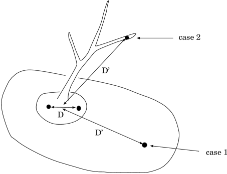
Figure 5: The observer operators at the geodesic distance $D^{\prime}$ from the two close operators. In case 1 the observer operator can be regarded to be outside the region surrounding the two close operators, whereas in case 2 it is at a definite distance $D^{\prime}$ because of a large fluctuation of the local degrees of freedom in the metric.

We expect OPE holds in case 1. As we will show in the remainder of this subsection, the calculations of the coefficients $C_{nm}^{~{}~{}~{}k}$ for $k\leq 6$ are affected only by configurations corresponding to the case 1, whereas those for $k\geq 7$ are affected by configurations of both the case 1 and the case 2. Therefore we can expect that OPE holds true for $k\leq 6$ but not for $k\geq 7$. We consider this as a natural explanation for the results in the previous subsection.

Let us then see how the above claim can be made. First, we will distinguish the two cases mentioned above definitely as follows. Let us consider a section of the surface at a geodesic distance $\tilde{D}$ from the union of the two close operators (See Fig. 6).

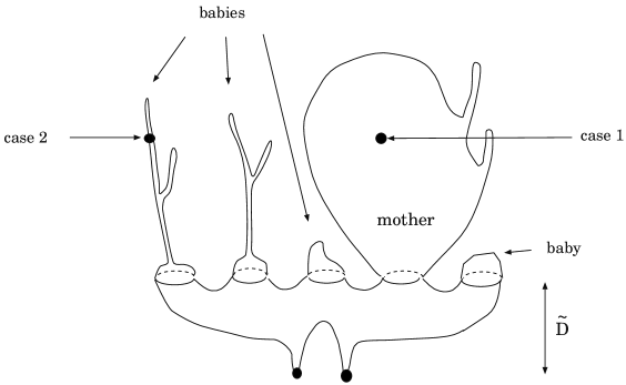
Figure 6: Two cases for the positions of the observer operators. The section of the surface at the geodesic distance $\tilde{D}$ from the union of the two close operators is composed of many loops, one of which is attached to the mother universe. The case 1 corresponds to the situation where the observer operator lies in the mother universe, while in the case 2 it lies in one of the baby universes.

We can take an arbitrary value for $\tilde{D}$ if it is greater than $D/2$ and smaller than $D^{\prime}$. The section is composed of many loops. It is known that only one of the loops is attached to the mother universe (infinite-volume universe) and the others are attached to baby universes (finite-volume universes) [10]. The case 1 corresponds to the situation where the observer operator lies in the mother universe, while in the case 2 it lies in one of the baby universes.

As in the previous subsection, let us consider the comparison between the three-point functions and the two-point functions. The case 2 corresponds to the configuration in Fig. 7, where the observer operator ${\cal O}_{l}$ is in a baby universe.

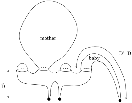
Figure 7: Configurations in the three-point functions corresponding to the case 2. The observer operator $O_{l}$ lies in a baby universe.

As we explained in Section 3, taking the thermodynamic limit corresponds to taking the term proportional to $t^{3/2}$. Since the contribution from the mother universe part is proportional to $t^{3/2}$, those from baby universe parts should be proportional to $t^{0}$. Hence, from dimensional analysis the baby universe part where the observer operator lies in Fig. 7 gives the factor

$$G_{jl}(D^{\prime}-\tilde{D};t=0)\sim(D^{\prime}-\tilde{D})^{-1-j-l}~{}~{}~{}~{}~{}(j=1,2,3,\cdots).$$ (4.18)

Therefore the configurations corresponding to the case 2 give only the power of $D^{\prime}$ lower than $D^{\prime}{}^{-2-l}$. As we can see from (4.16) and (4.17), these configurations only affects the calculations of the coefficients $C_{nm}^{~{}~{}~{}k}$ for $k\geq 7$.

Also in the general case in which we obtain $C_{nm}^{~{}~{}~{}k}$ by comparing the $N$-point functions and the $(N-1)$-point functions, we can show by dimensional analysis that the contribution of the configurations with some of the observers belonging to baby universes only affects the coefficients for $k\geq 7$.

In this way, we have explained why we obtained the consistent OPE coefficients for $k\leq 6$ and not for $k\geq 7$.

5 Summary and Discussion

In this paper, we have calculated the correlation functions with fixed geodesic distances up to three-point functions. We found that there are scaling operators ${\cal O}_{n}$ with even $n$, which can not be seen unless the geodesic distance is fixed. Elucidating why these new operators appear is an open problem. From the two-point functions of the cosmological constant terms with fixed geodesic distances, we were able to see the fractal structure of the space-time in a more direct way than it was seen through the loop-length distribution. We examined the OPE in quantum gravity, namely if two operators close to each other can be viewed as a superposition of operators when seen from a distance. By comparison of three-point and two-point functions, as well as by comparison of two-point and one-point functions, we obtained the OPE coefficients $C_{nm}^{~{}~{}~{}k}$, which are found to be consistent for $k\leq 6$.

This is because the calculations of the coefficients $C_{nm}^{~{}~{}~{}k}$ for $k\leq 6$ are affected only by the configurations where the observer operators lie in the mother universe. On the contrary, we obtained inconsistent results for $k\geq 7$ because they are affected by both configurations where the observer operators lie in the mother and the baby universes.

There are several things that need to be clarified further. First of all, we should calculate $N$-point functions with $N\geq 4$ in order to check further the consistency of the operator product expansion given in this paper. We should see if we can make the $C_{nm}^{~{}~{}~{}k}$ consistent for $k\geq 7$ as well by restricting all the observers to be in the mother universe. Considering higher genus and including matter degrees of freedom are also interesting extensions of our analysis.

We expect that operator product expansion holds in the case of higher-dimensional quantum gravity as well. We hope that this kind of approach will eventually enable us to understand the universality class of quantum gravity.

We would like to thank M. Oshikawa, M. Ikehara and N. Ishibashi for stimulating discussion. We are also grateful to N.D. Hari Dass for carefully reading the manuscript.

References

-
[1]
V.G. Knizhnik, A.M. Polyakov
and A.B. Zamolodchikov, Mod. Phys. Lett. A3 (1988) 819.
F. David, Mod. Phys. Lett. A3 (1988) 1651.
J. Distler and H. Kawai, Nucl. Phys. B321 (1989) 504.
E. Brezin and V. Kazakov, Phys. Lett. B236 (1990) 144.
M. Douglas and S. Shenker, Nucl. Phys. B335 (1990) 635.
D.J. Gross and A.A. Migdal, Phys. Rev. Lett. 64 (1990) 717; Nucl. Phys. B340 (1990) 333. -
[2]
M. Fukuma, H. Kawai and R. Nakayama, Int. J. Mod. Phys. A6
(1991) 1385.
R. Dijkgraaf, E. Verlinde and H. Verlinde, Nucl. Phys. B348 (1991) 435. -
[3]
S. Weinberg, in General Relativity, an Einstein Centenary
Survey, eds. S.W. Hawking and W. Israel
(Cambridge University Press, 1979).
R. Gastmans, R. Kallosh and C. Truffin, Nucl. Phys. B133 (1978) 417.
S.M. Christensen and M.J. Duff, Phys. Lett. B79 (1978) 213.
H. Kawai and M. Ninomiya, Nucl. Phys. B336 (1990) 115.
H. Kawai, Y. Kitazawa and M. Ninomiya, Nucl. Phys. B393 (1993) 280; Nucl. Phys. B404 (1993) 684.
T. Aida, Y. Kitazawa, H. Kawai and M. Ninomiya, Nucl. Phys. B427 (1994) 158.
T. Aida, Y. Kitazawa, J. Nishimura and A. Tsuchiya, Nucl. Phys. B444 (1995) 353. -
[4]
J. Nishimura, N. Tsuda and T. Yukawa,
Prog. Theor. Phys. Suppl. 114 (1993) 19.
R.L. Renken, Phys. Rev. D50 (1994) 5130.
R.L. Renken, S.M. Catterall and J.B. Kogut, Phys. Lett. B345 (1995) 422.
G. Thorleifsson, S. Catterall, A Real-Space Renormalization Group of Random Surfaces, SU-4240-619, hep-lat/9510003.
Z. Burda, J.-P. Kownacki and A. Krzywicki, Phys. Lett. B356 (1995) 466. - [5] I.R. Klebanov, I.I. Kogan and A.M. Polyakov, Phys. Rev. Lett. 71 (1993) 3243.
- [6] H. Kawai, N. Kawamoto, T. Mogami and Y. Watabiki, Phys. Lett. B306 (1993) 19.
- [7] N. Ishibashi and H. Kawai, Phys. Lett. B314 (1993) 190.
- [8] N. Ishibashi and H. Kawai, Phys. Lett. B322 (1994) 67.
-
[9]
J. Ambjorn and Y. Watabiki, Nucl. Phys. B445 (1995) 129.
J. Ambjorn, J. Jurkiewicz and Y. Watabiki, Nucl. Phys. B454 (1995) 313.
J. Ambjorn, Quantization of Geometry, hep-th/9411179. - [10] H. Kawai, Nucl. Phys. B (Proc. Suppl.) 26 (1992) 93.