KUNS-1368

HE(TH) 95/18

hep-th/9511033

July, 1994

The Universal Renormalization Factors  $Z_{1}/Z_{3}$
and Color Confinement Condition
in Non-Abelian Gauge Theory

Taichiro Kugo
Department of Physics, Kyoto University, Kyoto 606-01, Japan

The ratio $Z_{1}/Z_{3}$ of vertex and wave-function renormalization factors, which is universal (i.e., matter-independent), is shown to equal $1+u$ which gives the residue of the scalar pole $\propto p_{\mu}p_{\nu}/p^{2}$ of 2-point function $\left\langle\,{D_{\mu}c\,\,D_{\nu}\bar{c}}\,\right\rangle$. This relation is interesting since $1+u=0$ has been known to give a sufficient condition for color confinement. We also give an argument that, when $1+u=0$ holds, it will be realized by the disappearance of the massless gauge boson pole and is related with the restoration of a certain “local gauge symmetry” as was discussed by Hata.

1 Introduction

It is a well-known consequence of the Slavnov-Taylor identity that the ratio of vertex renormalization factor to wave-function renormalization factor is universal:

$${Z_{1}\over Z_{3}}={\widetilde{Z}_{1}\over\widetilde{Z}_{3}}={Z_{\bar{\psi}\psi A}\over Z_{\psi}}=\ \cdots\ ,$$ (1.1)

where the denominators $Z_{3}$, $\widetilde{Z}_{3}$ and $Z_{\psi}$ are the wave-function renormalization factors of gauge-boson, Faddeev-Popov ghost and matter field $\psi$, respectively, and the numerators $Z_{1}$, $\widetilde{Z}_{1}$ and $Z_{\bar{\psi}\psi A}$ are the gauge-boson vertex renormalization factors of those fields. Namely, the ratio is independent of the measured matter fields (and equals 1 in the QED case as a result of the Ward identity). [We may, however, have to keep in mind that it is gauge-dependent.]

The main purpose of this talk is to show that the following equality holds for this universal renormalization factor $Z_{1}/Z_{3}$ generally in covariant gauges (with arbitrary gauge parameter $\alpha$):

$${Z_{1}\over Z_{3}}=1+u\ ,$$ (1.2)

where $u\equiv u(p^{2}\!=\!0)$ and $u(p^{2})$ is the function defined by

$$\int d^{4}x\,e^{ipx}\left\langle{0}\right|{\rm T}D_{\mu}c^{a}(x)\,D_{\nu}\bar{c}^{b}(0)\left|{0}\right\rangle=\left[\Bigl{(}g_{\mu\nu}-{p_{\mu}p_{\nu}\over p^{2}}\Bigr{)}u(p^{2})-{p_{\mu}p_{\nu}\over p^{2}}\right]\delta_{ab}\ .$$ (1.3)

This relation (1.2) is very interesting since it is known[1] that $1+u=0$ gives a sufficient condition for all the colored states to become unphysical; namely,

$$1+u=0\quad\Longrightarrow\quad\hbox{Color Confinement}\,!$$ (1.4)

As a preparation for it, we briefly explain in Sect. 2 why the condition $1+u=0$ implies the color confinement. And then in Sect. 3 we give a proof of the relation (1.2). Some implications are discussed in Sect. 4, where I give an argument that the confinement condition $1+u=0$ implies the disappearance of the massless (vector) gauge boson pole. It, therefore, turns to imply that a certain “local gauge symmetry” is dynamically restored as was discussed by Hata[7]. This is explained in Sect. 5. The final Sect. 6 is devoted to some further discussions.

2 $1+u=0$: A Color Confinement Condition

Let us first recapitulate how the condition $1+u=0$ is related to the color confinement[1]. As noted by Ojima[2] first, the equation of motion for the gauge field can be written in the following form of Maxwell-type:

$$gJ_{\mu}^{a}=\partial^{\nu}F_{\mu\nu}^{a}+\{Q_{\rm B},\,D_{\mu}\bar{c}^{a}\}\ ,$$ (2.1)

where $J_{\mu}^{a}$ is the Noether current of color symmetry (global gauge symmetry). The point is that the Noether current always has an arbitrariness adding a term of the form $\partial^{\nu}f_{[\mu\nu]}$ with an arbitrary local anti-symmetric tensor $f_{[\mu\nu]}$. That is, the modified current $J_{\mu}^{{}^{\prime}a}\equiv J_{\mu}^{a}+\partial^{\nu}f_{[\mu\nu]}$ is still conserved and, moreover, the corresponding charge generates the infinitesimal color rotation correctly on any field operators (at least with formal application of canonical commutation relations). We have, therefore, a possibility to define the color charge $Q^{a}$ by

$$Q^{a} = \int d^{3}x\,\Bigl{(}J_{\mu}^{a}-{1\over g}\partial^{\nu}F_{\mu\nu}^{a}\Bigr{)}_{\mu=0}$$ (2.2)

$$= \int d^{3}x\,{1\over g}\big{\{}Q_{\rm B},\,D_{\mu}\bar{c}^{a}\big{\}}_{\mu=0}$$

If we could define the color charge by this equation, then it takes a BRS-exact form and so the color confinement is concluded: indeed, for any physical states $\left|{{\rm phy}}\right\rangle$ specified by the condition $Q_{\rm B}\left|{{\rm phys}}\right\rangle=0$, we have

$$\left\langle{{\rm phys}}\right|Q^{a}\left|{{\rm phys}^{\prime}}\right\rangle=0\ .$$ (2.3)

It is an easy exercise to show from this equation that all the physical (that is, BRS-singlet) particles are color-singlet[1].

The expression Eq. (2.2), however, does not give a well-defined color charge operator generally. This is because there is a massless one-particle contribution to $J_{\mu}^{a}$, $\partial^{\nu}F_{\mu\nu}^{a}$ and $\{Q_{\rm B},\,D_{\mu}\bar{c}^{a}\}$ so that the 3-volume integration does not converge. To show this, we have first to explain the elementary quartet (a quartet = a pair of BRS-doublets).

We can easily show that there always exists a massless quartet for each group index $a$. Indeed, using the equation of motion $\partial^{\mu}D_{\mu}c^{a}=0$ and equal time anti-commutation relation, we find an identity

$$\partial^{\mu}_{x}\left\langle{0}\right|{\rm T}D_{\mu}c^{a}(x)\,\bar{c}^{b}(y)\left|{0}\right\rangle=\delta^{ab}\delta^{4}(x-y)\ ,$$ (2.4)

implying that

$$\int d^{4}x\,e^{ipx}\left\langle{0}\right|{\rm T}D_{\mu}c^{a}(x)\,\bar{c}^{b}(0)\left|{0}\right\rangle=i\delta^{ab}{p_{\mu}\over p^{2}}\ .$$ (2.5)

But, an identity $\left\langle{0}\right|\{Q_{\rm B},{\rm T}(A_{\mu}^{a}\,\bar{c}^{b})\}\left|{0}\right\rangle=0$ means the Ward-Takahashi identity

$$i\left\langle{0}\right|{\rm T}D_{\mu}c^{a}(x)\,\bar{c}^{b}(y)\left|{0}\right\rangle=\left\langle{0}\right|{\rm T}A_{\mu}^{a}(x)\,B^{b}(y)\left|{0}\right\rangle\ ,$$ (2.6)

so that Eq. (2.5) implies also an identity:

$$\int d^{4}x\,e^{ipx}\left\langle{0}\right|{\rm T}A_{\mu}^{a}(x)\,B^{b}(0)\left|{0}\right\rangle=-\delta^{ab}{p_{\mu}\over p^{2}}\ .$$ (2.7)

The identities (2.5) and (2.7) give exact Green functions and so the presence of massless pole $\propto 1/p^{2}$ implies that the following four massless asymptotic fields $\gamma^{a}$, $\bar{\gamma}^{a}$, $\chi^{a}$ and $\beta^{a}$ exist for each group index $a$:

$$D_{\mu}c^{a}(x) \mathrel{\mathop{\kern 0.0pt\relbar\kern-3.0pt\longrightarrow}\limits_{x_{0}\rightarrow\pm\infty}} \partial_{\mu}\gamma^{a}(x)+\cdots$$

$$\bar{c}^{a}(x) \longrightarrow \bar{\gamma}^{a}(x)+\cdots$$

$$A_{\mu}^{a}(x) \longrightarrow \partial_{\mu}\chi^{a}(x)+\cdots$$

$$B^{a}(x) \longrightarrow \beta^{a}(x)+\cdots\ .$$ (2.8)

From BRS transformation law $[iQ_{\rm B},\,A_{\mu}^{a}]=D_{\mu}c^{a}$ and $\{Q_{\rm B},\,\bar{c}^{a}\}=B^{a}$, we find that these asymptotic fields transform as follows under the BRS transformation:

$$[iQ_{\rm B},\,\chi^{a}(x)]=\gamma^{a}(x)\ ,\qquad\{Q_{\rm B},\,\bar{\gamma}^{a}(x)\}=\beta^{a}(x)\ .$$ (2.9)

This clearly shows that these asymptotic fields $\gamma^{a}$, $\bar{\gamma}^{a}$, $\chi^{a}$ and $\beta^{a}$ really forms a BRS quartet representation.

Now we come back to the well-definedness problem of the expression Eq. (2.2). The point is that $D_{\mu}\bar{c}^{a}=\partial_{\mu}\bar{c}^{a}+g(A_{\mu}\times\bar{c})^{a}$ generally contains the one-particle contribution of the massless asymptotic field $\bar{\gamma}^{a}$:

$$D_{\mu}\bar{c}^{a}=\partial_{\mu}\bar{c}^{a}+g(A_{\mu}\times\bar{c})^{a}\quad\longrightarrow\quad(1+u)\partial_{\mu}\bar{\gamma}^{a}\ ,$$ (2.10)

where the weight 1 comes from the first term $\partial_{\mu}\bar{c}^{a}$ and the weight $u$ from the second $g(A_{\mu}\times\bar{c})^{a}$. This can be seen by looking at the definition (1.3) of $u$ and Eq. (2.5). We thus see that the operator $\{Q_{\rm B},\,D_{\mu}\bar{c}^{a}\}$ contains the massless one-particle contribution of the elementary quartet member $\beta^{a}$ in the form

$$\big{\{}\,Q_{\rm B},\,D_{\mu}\bar{c}^{a}(x)\,\big{\}}\quad\mathrel{\mathop{\kern 0.0pt\relbar\kern-3.0pt\longrightarrow}\limits_{x_{0}\rightarrow\pm\infty}}\quad(1+u)\partial_{\mu}\beta^{a}(x)\ .$$ (2.11)

Generally, the other operators $J_{\mu}^{a}$ and $\partial^{\nu}F_{\mu\nu}^{a}$ appearing in the Maxwell equation (2.1) also have the one-particle contributions from $\beta^{a}$ since they carry the same quantum numbers as $\{Q_{\rm B},\,D_{\mu}\bar{c}^{a}\}$:

$$J_{\mu}^{a}(x)\quad\longrightarrow\quad v\partial_{\mu}\beta^{a}(x)\ ,\qquad\partial^{\nu}F_{\mu\nu}^{a}(x)\quad\longrightarrow\quad-w\partial_{\mu}\beta^{a}(x)\ ,$$ (2.12)

with suitable weights $v$ and $w$. In QED, one can easily see that $u=0$ and $w=Z_{3}$. The Maxwell equation (2.1) tells us the relation between those weights:

$$gv=-w+(1+u)\ .$$ (2.13)

The well-defined color charge is, therefore, given by

$$Q^{a}=\int d^{3}x\,\Bigl{(}J_{\mu}^{a}+{v\over w}\partial^{\nu}F_{\mu\nu}^{a}\Bigr{)}_{\mu=0}\ ,$$ (2.14)

so that the massless one-particle contribution $\partial_{\mu}\beta^{a}$ contained in $J_{\mu}^{a}$ is cancelled by that in $\partial^{\nu}F_{\mu\nu}^{a}$.

Now, if the condition $1+u=0$ holds, then we have $v/w=-1/g$ and so the well-defined color charge Eq. (2.14) happens to coincide with the previous BRS-exact expression (2.2) implying the color confinement.

3 Proof of the relation $Z_{1}/Z_{3}=1+u$

I have noticed this relation $Z_{1}/Z_{3}=1+u$ for the first time in studying the renormalization problem in the background field method in collaboration with Imamura and Van Proeyen[3]. However, the proof by that method is a bit complicated and so here I will give a simpler proof using a similar method to Aoki’s[4] which he used when proving the electro-magnetic charge universality in the Weinberg-Salam model.

Add $g(v/w)\partial^{\nu}F_{\mu\nu}^{a}$ to both sides of the Maxwell equation (2.1), and then we have

$$gJ_{\mu}^{a,\rm well\hbox{-}def}=\Bigl{(}1+g{v\over w}\Bigr{)}\partial^{\nu}F_{\mu\nu}^{a}+\{Q_{\rm B},\,D_{\mu}\bar{c}^{a}\}\ ,$$ (3.1)

with

$$J_{\mu}^{a,\rm well\hbox{-}def}\equiv J_{\mu}^{a}+{v\over w}\partial^{\nu}F_{\mu\nu}^{a}$$ (3.2)

being the color current giving the well-defined color charge (2.14). Using a relation $1+gv/w=(1+u)/w$ following from Eq. (2.13), we find

$${1+u\over w}\partial^{\nu}F_{\mu\nu}^{a}=gJ_{\mu}^{a,\rm well\hbox{-}def}-\{Q_{\rm B},\,D_{\mu}\bar{c}^{a}\}\ .$$ (3.3)

Sandwitching this with two physical states $\left\langle{f}\right|$ and $\left|{g}\right\rangle$ satisfying $\left\langle{f}\right|Q_{\rm B}=Q_{\rm B}\left|{g}\right\rangle=0$, yields

$${1+u\over w}\partial^{\nu}\left\langle{f}\right|F_{\mu\nu}^{a}(x)\left|{g}\right\rangle=g\left\langle{f}\right|J_{\mu}^{a,\rm well\hbox{-}def}(x)\left|{g}\right\rangle\ .$$ (3.4)

We now make an operation $\lim_{p\rightarrow 0}\int d^{4}x\,e^{ipx}$ act on both sides of this equation and evaluate the both sides separately. Start with the left-hand side. Because of the presence of the divergence $\partial^{\nu}$, only massless one-particle pole contribution to the matrix element $\left\langle{f}\right|F_{\mu\nu}^{a}(x)\left|{g}\right\rangle$ can survive in this limit. But such a massless one-particle pole (if any) comes from the gauge boson contribution as shown in Fig. 1

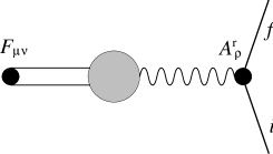
Figure 1: Diagram of massless pole contribution.

and generally takes the form

$$\int d^{4}x\,e^{ipx}\left\langle{f}\right|F_{\mu\nu}^{a}(x)\left|{g}\right\rangle\Big{|}_{\rm pole\ part}=\left\langle\,{F_{\mu\nu}^{a}\,A^{b}_{{\rm r},\rho}}\,\right\rangle V^{\rho,b}_{fi}\ ,$$

$$\quad\left\langle\,{F_{\mu\nu}^{a}\,A^{b}_{{\rm r},\rho}}\,\right\rangle=-Y{p_{\mu}g_{\nu\rho}-p_{\nu}g_{\mu\rho}\over p^{2}}\delta_{ab}\ ,$$

$$\quad V^{\rho,b}_{fi}=ig_{\rm r}T^{b}_{fi}(p_{f}+p_{i})^{\rho}(2\pi)^{4}\delta^{4}(p+p_{f}-p_{i})\ ,$$ (3.5)

where $\left\langle\,{F_{\mu\nu}^{a}\,A^{b}_{{\rm r},\rho}}\,\right\rangle$ stands for the propagator from $F_{\mu\nu}^{a}$ to the renormalized gauge boson $A^{b}_{{\rm r},\rho}$, and $V^{\rho,b}_{fi}$ for the vertex of the renormalized gauge boson between the on-shell initial and final states. $Y$ is a weight factor and $g_{\rm r}$ is the renormalized coupling constant. Substituting this expression, we find that the left-hand side becomes

$$-Y{1+u\over w}\lim_{p\rightarrow 0}\Bigl{(}-i{p_{\mu}p_{\rho}\over p^{2}}+ig_{\mu\rho}\Bigr{)}(ig_{\rm r})T^{a}_{fi}(p_{f}+p_{i})^{\rho}(2\pi)^{4}\delta^{4}(p+p_{f}-p_{i})\ .$$ (3.6)

Noting the pole term $p_{\mu}p_{\rho}/p^{2}$ vanishes owing to the “current conservation” at the vertex, we obtain

$${1+u\over w}\lim_{p\rightarrow 0}\int d^{4}x\,e^{ipx}\partial^{\nu}\left\langle{f}\right|F_{\mu\nu}^{a}(x)\left|{g}\right\rangle$$

$$\qquad\qquad\qquad\ =\ Y{1+u\over w}g_{\rm r}T^{a}_{fi}\lim_{p_{f}\rightarrow p_{i}}(p_{f}+p_{i})_{\mu}(2\pi)^{4}\delta^{4}(p_{f}-p_{i})\ .$$ (3.7)

The weight factor $Y$ introduced in Eq. (3.5) can easily be related to the previous weight $w$: using $\partial^{\nu}F_{\mu\nu}^{a}(x)\longrightarrow-w\partial_{\mu}\beta^{a}(x)$ and the WT identity (2.7) with $A_{{\rm r},\rho}^{b}=Z_{3}^{-1/2}A_{\rho}^{b}$, we obtain

$$\left\langle\,{\partial^{\nu}F_{\mu\nu}^{a}\,A_{{\rm r},\rho}^{b}}\,\right\rangle\Big{|}_{\rm pole\ part}=-w\left\langle\,{\partial_{\mu}B^{a}\,A_{{\rm r},\rho}^{b}}\,\right\rangle=wZ_{3}^{-1/2}(i\delta^{ab}){p_{\mu}p_{\rho}\over p^{2}}\ ,$$ (3.8)

comparison of which with the divergence of the second equation in Eq. (3.5) leads to

$$Y=wZ_{3}^{-1/2}\ ,\qquad\hbox{so that}\qquad Y{1+u\over w}=(1+u)Z_{3}^{-1/2}.$$ (3.9)

The right hand side of Eq. (3.4), on the other hand, can be easily evaluated for $\mu=0$ component as follows:

$$\lim_{p\rightarrow 0}\int d^{4}x\,e^{ipx}g\left\langle{f}\right|J_{0}^{a,\rm well\hbox{-}def}(x)\left|{g}\right\rangle = \int dx_{0}\,g\left\langle{f}\right|Q^{a,\rm well\hbox{-}def}\left|{g}\right\rangle$$ (3.10)

$$= gT^{a}_{fi}\lim_{p_{f}\rightarrow p_{i}}2p_{i}^{0}(2\pi)^{4}\delta^{4}(p_{f}-p_{i})\ .$$

Now comparing this with the above Eq. (3.7) with Eq. (3.9), we finally obtain a relation

$$(1+u)Z_{3}^{-1/2}g_{\rm r}=g\ .$$ (3.11)

But, if we use the relation $g=Z_{1}Z_{3}^{-3/2}g_{\rm r}$ between the bare and renormalized coupling constants $g$ and $g_{\rm r}$, this is nothing but the desired relation $1+u=Z_{1}/Z_{3}$, Eq. (1.2).

We have proved the relation $1+u=Z_{1}/Z_{3}$ in covariant gauges with arbitrary values of gauge parameter $\alpha$. In Landau gauge $\alpha=0$, however, it is easier to show it. First define the following two-point functions

$$\left\langle\,{c\,\,\bar{c}}\,\right\rangle \equiv -{1\over p^{2}G(p^{2})}\ ,$$

$$\left\langle\,{g(A_{\mu}\!\!\times\!c)\,\,\bar{c}}\,\right\rangle_{\rm 1PI} \equiv \left\langle\,{g(A_{\mu}\!\!\times\!c)\,\,\bar{c}}\,\right\rangle/\left\langle\,{c\,\,\bar{c}}\,\right\rangle\equiv-ip_{\mu}F(p^{2})\ .$$ (3.12)

Here and henceforth we use an abbreviated notation:

$$\left\langle\,{\,A\,B\,}\,\right\rangle\equiv\int d^{4}x\,e^{ipx}\left\langle{0}\right|{\rm T}\,A(x)\,B(0)\left|{0}\right\rangle\ .$$ (3.13)

The suffix 1PI generally denotes the one-particle irreducible vertex. Then, we have

$$\left\langle\,{D_{\mu}c\,\,\bar{c}}\,\right\rangle=\left\langle\,{\partial_{\mu}c\,\,\bar{c}}\,\right\rangle+\left\langle\,{g(A_{\mu}\!\!\times\!c)\,\,\bar{c}}\,\right\rangle\equiv ip_{\mu}\big{(}1+F(p^{2})\big{)}{1\over p^{2}G(p^{2})}\ .$$ (3.14)

But this must equal $ip^{\mu}/p^{2}$ because of Eq. (2.7) so that

$$1+F(p^{2})=G(p^{2})\ .$$ (3.15)

On the other hand, a simple diagramatical consideration shows that

$$\left\langle\,{c\,\,g(A_{\nu}\!\!\times\!\bar{c})}\,\right\rangle_{\rm 1PI}=ip^{\rho}\left\langle\,{g(A_{\rho}\!\!\times\!c)\,\,g(A_{\nu}\!\!\times\!\bar{c})}\,\right\rangle_{\rm 1PI}$$ (3.16)

and hence that

$$\left\langle\,{D_{\mu}c\,\,g(A_{\nu}\!\!\times\!\bar{c})}\,\right\rangle = \left\langle\,{D_{\mu}c\,\,\bar{c}}\,\right\rangle\,\left\langle\,{c\,\,g(A_{\nu}\!\!\times\!\bar{c})}\,\right\rangle_{\rm 1PI}+\left\langle\,{g(A_{\mu}\!\!\times\!c)\,\,g(A_{\nu}\!\!\times\!\bar{c})}\,\right\rangle_{\rm 1PI}$$ (3.17)

$$= \Bigl{(}\delta_{\mu}^{\rho}-{p_{\mu}p^{\rho}\over p^{2}}\Bigr{)}\left\langle\,{g(A_{\rho}\!\!\times\!c)\,\,g(A_{\nu}\!\!\times\!\bar{c})}\,\right\rangle_{\rm 1PI}\ .$$

The last Green function $\left\langle\,{D_{\mu}c\,\,g(A_{\nu}\!\!\times\!\bar{c})}\,\right\rangle$ must be equal to $\big{(}g_{\mu\nu}-(p_{\mu}p_{\nu}/p^{2})\big{)}u(p^{2})$ because of the definition (1.3) of the function $u(p^{2})$ so that $\left\langle\,{g(A_{\mu}\!\!\times\!c)\,\,g(A_{\nu}\!\!\times\!\bar{c})}\,\right\rangle_{\rm 1PI}$ have to have the form

$$\left\langle\,{g(A_{\mu}\!\!\times\!c)\,\,g(A_{\nu}\!\!\times\!\bar{c})}\,\right\rangle_{\rm 1PI}=g_{\mu\nu}u(p^{2})+p_{\mu}p_{\nu}v(p^{2})$$ (3.18)

with $v(p^{2})$ being an arbitrary function. Up to here all the equations hold for any covariant $\alpha$ gauges. But, in Landau gauge $\alpha=0$, we have additionally an identity

$$-ip_{\mu}F(p^{2}) \equiv \left\langle\,{g(A_{\mu}\!\!\times\!c)\,\,\bar{c}}\,\right\rangle_{\rm 1PI}$$ (3.19)

$$\equiv \left\langle\,{g(A_{\mu}\!\!\times\!c)\,\,g(A_{\nu}\!\!\times\!\bar{c})}\,\right\rangle_{\rm 1PI}\times(-ip^{\nu})\ .$$

This is because the derivative factor acting on the anti-ghost at the $\bar{c}$-$A_{\nu}$-$c$ vertex at the right end of the diagrams can be transferred to act on the external ghost since $\partial_{\nu}A^{\nu}=0$ in the Landau gauge. Therefore we have

$$-ip_{\mu}F(p^{2})=-ip_{\mu}\Bigl{(}u(p^{2})+p^{2}v(p^{2})\Bigr{)}\ ,\quad\Longrightarrow\quad G(p^{2})-1=u(p^{2})+p^{2}v(p^{2})\ .$$ (3.20)

This relation yields at $p^{2}=0$

$$G(0)=1+u(0)\ ,$$ (3.21)

but, since $G(0)=\widetilde{Z}_{3}^{-1}$ and $\widetilde{Z}_{1}=1$ in the Landau gauge, this shows the relation $\widetilde{Z}_{1}/\widetilde{Z}_{3}=1+u$, thus proving the desired identity Eq. (1.2).

4 What Does $1+u=Z_{1}/Z_{3}$ Imply?

How is $1+u=Z_{1}/Z_{3}=0$ expected to be realized? Naively, we immediately expect the following two possibilities:
          1.  $Z_{1}=0$, and $Z_{3}={}$finite.
          2.  $Z_{1}={}$finite, and $Z_{3}=0$.
However, since the condition is concerned with only the ratio, we have, for instance, even the possibility
          3.  $Z_{3}=0$, but/and $Z_{1}/Z_{3}=0$.
Here I mean that $Z_{1}$ has a higher zero than $Z_{3}$; e.g., $Z_{3}(p^{2})={\cal O}(p^{2})$ and $Z_{1}(p^{2})={\cal O}(p^{4})$. The wave-function renormalization factor $Z_{3}(p^{2})$ as a function of $p^{2}$ can be defined as follows by the general form of gauge boson 2-point function:

$$\int d^{4}x\,e^{ipx}\left\langle{0}\right|{\rm T}\,A_{\mu}^{a}(x)\,A_{\nu}^{b}(x)\left|{0}\right\rangle=\left[\Bigl{(}g_{\mu\nu}-{p_{\mu}p_{\nu}\over p^{2}}\Bigr{)}{Z_{3}(p^{2})\over p^{2}}+\alpha{p_{\mu}p_{\nu}\over p^{4}}\right]\delta^{ab}$$ (4.1)

Although I cannot prove it, it seems plausible that the possibility 3 is realized when $1+u=0$. Let us now explain this.

Assume that $Z_{3}(p^{2}\!=\!0)\not=0$, then, there exists a vector asymptotic field ${\cal A}^{a}_{\mu}(x)$ in the channel $A_{\mu}^{a}(x)$:

$$A_{\mu}^{a}(x)\quad\mathrel{\mathop{\kern 0.0pt\relbar\kern-3.0pt\longrightarrow}\limits_{x_{0}\rightarrow\pm\infty}}\quad{\cal A}^{a}_{\mu}(x)\ .$$ (4.2)

This is a colored particle. But any colored particles are confined when $1+u=0$. Therefore the BRS transform of $A_{\mu}^{a}(x)$

$$[iQ_{\rm B},\,A_{\mu}^{a}(x)]=D_{\mu}c^{a}(x)\ ,$$ (4.3)

with ghost number 1, should also have its own massless vector asymptotic field ${\cal C}^{a}_{\mu}(x)$ such that $\big{(}{\cal A}^{a}_{\mu}(x),\,{\cal C}^{a}_{\mu}(x)\big{)}$ form a BRS-doublet (and hence become unphysical):

$$[iQ_{\rm B},\,{\cal A}_{\mu}^{a}(x)]={\cal C}^{a}_{\mu}(x)\ .$$ (4.4)

This is a color confinement by the quartet mechanism[5]. Since this asymptotic field ${\cal C}^{a}_{\mu}(x)$ is a vector, it must be a bound-state in the $(A_{\mu}\times c)^{a}$ channel. So it is natural to suppose that it should show up as a pole in the 1PI Green function $\left\langle\,{g(A_{\mu}\!\!\times\!c)\,\,g(A_{\nu}\!\!\times\!\bar{c})}\,\right\rangle_{\rm 1PI}$, namely, in Eq. (3.18)

$$\left\langle\,{g(A_{\mu}\!\!\times\!c)\,\,g(A_{\nu}\!\!\times\!\bar{c})}\,\right\rangle_{\rm 1PI}=g_{\mu\nu}u(p^{2})+p_{\mu}p_{\nu}v(p^{2})\ .$$

The vector massless pole $1/p^{2}$ should appear in the $g_{\mu\nu}$-part, i.e., in $u(p^{2})$. But this contradicts with the present assumption $u=u(p^{2}\!=\!0)=1$.

This argument, therefore, suggests that the massless vector pole in $A_{\mu}^{a}$, which existed in the perturbation phase, should disappear (or the appearance of mass gap): namely,

$$Z_{3}(p^{2})\propto p^{2}\ ,$$ (4.5)

corresponding to the above possibility 3.

5 Dynamical Restoration of a “Local” Gauge Symmetry

The conclusion in the previous section reminds me Hata’s work[7, 8] who clarified a symmetry aspect of the ‘strange’ condition $1+u=0$. So let us briefly recapitulate what he has done in this context.

In QED, the covariant $\alpha$ gauge fixing still leaves a symmetry under the gauge transformation with transformation parameter linear in $x$:

$$\Lambda(x)=a_{\nu}x^{\nu}+b\ .$$ (5.1)

Although being a (special) “local” gauge symmetry, this transformation can be regarded as a combination of global transformations with $x$-independent parameters $a_{\nu}$ and $b$. We have accordingly conserved Noether charges, vector one $Q^{\nu}$ and scalar one $Q$, (the latter $Q$ being just a usual electro-magnetic (global $U(1)$) charge), and they give the generators of the original transformation:

$$[\,i(a_{\nu}Q^{\nu}+bQ),\,A_{\mu}(x)\,]=\partial_{\mu}\Lambda(x)=a_{\mu}\ ,$$

$$\qquad\qquad\Longrightarrow\quad\cases{[\,iQ,\,A_{\mu}(x)\,]=0\cr[\,iQ^{\nu},\,A_{\mu}(x)\,]=\delta_{\mu}^{\nu}\cr}$$ (5.2)

The first commutation relation says only that the photon $A_{\mu}$ carries vanishing charge, but the second one shows that the vector symmetry of charge $Q^{\nu}$ is always spontaneously broken since the right-hand side is non-vanishing c-number $\delta_{\mu}^{\nu}$ ! It also says that the massless Nambu-Goldstone (NG) mode corresponding to the spontaneous breaking should appear in the $A_{\mu}$ channel. It can be argued that, as far as the global $U(1)$ symmetry corresponding to the scalar charge $Q$ is not spontaneously broken, the NG mode must be a vector particle so that the photon can be identified with the Nambu-Goldstone vector[9]! [This type of argument is important since it proves the existence and exact masslessness of the photon. Quite a parallel argument can apply to gravity[10, 11] and proves the existence and exact masslessness of the graviton.]

Hata considered the same thing in non-Abelian gauge theory. Corresponding to the “local” gauge transformation,

$$\Lambda^{a}(x)=a_{\nu}^{a}x^{\nu}+b^{a}\ ,$$ (5.3)

there appear the following scalar and vector charges, both of which carry color index $a$ now:

$$Q^{a}\quad \longrightarrow \quad J_{\mu}^{a}(x)\ ,$$

$$Q^{a,\nu}\quad \longrightarrow \quad J_{\mu}^{a,\nu}(x)=gJ_{\mu}^{a}(x)x^{\nu}+F_{\mu}^{a\ \nu}\ .$$ (5.4)

In this case, however, the vector transformation with parameter $a_{\nu}^{a}$ is not an exact symmetry but is slightly violated and so

$$\partial^{\mu}J_{\mu,\nu}^{a}(x)=\big{\{}Q_{\rm B},\,D_{\nu}\bar{c}^{a}\big{\}}\ .$$ (5.5)

In his second paper[8], Hata considered a modified vector transformation which becomes an exact symmetry. But here we continue to consider the present simplified version. Again, this “local symmetry” with parameter $a_{\nu}^{a}x^{\nu}$ is spontaneously broken in the perturbation phase and the usual perturb-ative massless gauge boson can be identified with Nambu-Goldstone vector.

Contrary to the QED case, however, there is a possibility that this “local symmetry” is restored dynamically in the non-Abelian case. Hata’s picture for the color confinement is as follows:

Dynamical restoration of the “local symmetry” with parameter $$a_{\nu}^{a}x^{\nu}$$

$$\quad=\quad\hbox{Disordered phase}\quad=\quad\hbox{Confinement phase}\ .$$ (5.6)

Indeed, if the “local symmetry” is dynamically restored, then the massless vector pole (i.e., perturbative gauge boson pole) in the current $J^{a}_{\mu,\nu}$ should disappear and it will have no massless pole contribution. This requirement actually leads to the above condition $1+u=0$ of ours, since we have

$$\partial^{\mu}\left\langle\,{\,J_{\mu,\nu}^{a}(x)\,\,A_{\rho}^{b}\,}\,\right\rangle=i\Bigl{(}g_{\mu\rho}-{p_{\mu}p_{\rho}\over p^{2}}\Bigr{)}\bigl{(}1+u(p^{2})\bigr{)}\ .$$ (5.7)

Namely our condition $1+u=0$ is a necessary condition for the restoration of the “local symmetry”. I do not know whether it is also sufficient, but our discussion in the previous section strongly suggests that it is. Hata also gave another interesting direct proof that any colored particle has to be a BRS-doublet if the current $J_{\mu,\nu}^{a}(x)$ has no massless pole, by considering a 3-point Green function of $J_{\mu,\nu}^{a}(x)$ and the two fields corresponding to that colored particle[7].

6 Discussions

One may wonder how it is possible at all to satisfy our confinement condition $1+u=0$. This question is quite natural if we note the fact that $u=u(p^{2}\!=\!0)$ is both infrared and ultraviolet divergent in perturbation theory!

However, we should recall that quite a similar thing is actually realized in the non-linear sigma models in two dimension. As an example, consider the following $O(N)/O(N-1)$ sigma model again following Hata[7]:

$${\cal L}={1\over 2}{(\partial\mbox{\boldmath$\phi$})^{2}\over\Bigl{(}1+{\displaystyle{\lambda\over 4}}\mbox{\boldmath$\phi$}^{2}\Bigr{)}^{2}}\ ,\qquad\qquad\mbox{\boldmath$\phi$}\equiv\pmatrix{\phi_{1}\cr\vdots\cr\phi_{N-1}\cr}\ .$$ (6.1)

The non-linearly realized $O(N)/O(N-1)$ symmetry is the transformation:

$$\delta_{i}\phi_{j}=\Bigl{(}1-{\lambda\over 4}\mbox{\boldmath$\phi$}^{2}\Bigr{)}\delta_{ij}+{\lambda\over 2}\phi_{i}\phi_{j}\ ,$$ (6.2)

with $i=1,\ 2,\ \cdots,\ N-1$. In perturbation phase, this non-linear symmetry is (spontaneously) broken and the fields $\phi_{i}$ are the corresponding massless NG bosons. The restoration condition for this symmetry is given by, in the leading order in $1/N$ expansion,

$$\left\langle\,{\delta_{i}\phi_{j}}\,\right\rangle=\delta_{ij}\Bigl{(}1-{\lambda\over 4}\left\langle{\mbox{\boldmath$\phi$}^{2}}\right\rangle\Bigr{)}=0\ {}.$$ (6.3)

This is quite analogous to our condition $1+u=0$. The vacuum expectation value $-(\lambda/4)\left\langle{\mbox{\boldmath$\phi$}^{2}}\right\rangle$ corresponds to our $u$, and is indeed both infrared and ultraviolet divergent in perturbation calculation! Nevertheless we know[12] that $\bigl{(}1-\lambda\left\langle{\mbox{\boldmath$\phi$}^{2}}\right\rangle/4\bigr{)}$ is actually realized in this model. It is known rather generally that a mass gap appears and the nonlinear symmetry is dynamically restored in a wide variety of two dimensional non-linear sigma models.

As a matter of fact, this resemblance of dynamical symmetry restorations between Yang-Mills gauge theory in four dimension and non-linear sigma model in two dimension, is not a mere analogy. Indeed, it becomes an exact correspondence if we consider a pure gauge model of Yang-Mills theory in four dimension[13]. Let us close this talk by briefly explaining this.

Take the $SU(N)$ Yang-Mills theory with $OSp(4|2)$ symmetric gauge fixing:

$${\cal L}=-{1\over 4}F_{\mu\nu}^{2}+\delta_{\rm B}\bar{\delta}_{\rm B}\Bigl{(}{1\over 2}A_{\mu}^{2}+i\bar{c}c\Bigr{)}$$ (6.4)

where $\delta_{\rm B}$ and $\bar{\delta}_{\rm B}$ denote BRS and anti-BRS transformations, respectively. The pure gauge model is given by replacing the gauge field $A_{\mu}^{a}$ in this Lagrangian by the pure gauge mode $g^{\dagger}\partial_{\mu}g$:

$$A_{\mu}(x)\qquad\longrightarrow\qquad g^{\dagger}(x)\partial_{\mu}g(x)\ .$$ (6.5)

Then, the $F_{\mu\nu}^{2}$ term drops out and only the gauge-fixing term remains. Namely the pure gauge model is a kind of topological model. One can show very easily that this model is exactly equivalent by the Parisi-Sourlas mechanism to the two dimensional $SU(N)_{\rm L}\times SU(N)_{\rm R}/SU(N)$ non-linear sigma model with the action

$$\int d^{2}x\,\hbox{tr}\bigl{(}\partial^{\mu}g^{\dagger}\partial_{\mu}g\big{)}\ .$$ (6.6)

This model has an $SU(N)_{\rm L}\times SU(N)_{\rm R}$ symmetry under the transformation $g\rightarrow h_{\rm L}^{\dagger}gh_{\rm R}$. Very interestingly, the current corresponding to the $SU(N)_{\rm R}$ symmetry is found to be given by

$$J_{{\rm R}\,\mu}^{a}=\big{\{}Q_{\rm B},\,D_{\mu}\bar{c}^{a}\big{\}}\ .$$ (6.7)

So, if the symmetry is restored, then it implies that our condition $1+u=0$ is literally realized. This is what actually occurs as we know from the exact result due to Polyakov and Wiegmann[14]. So this pure gauge model has a possibility to be used as a “zeroth order” theory in a new form of “perturbation theory” in the actual non-Abelian gauge theory, in which the confinement condition $1+u=0$ is satisfied order by order. It is encouraging that such trials towards this direction are already performed by several authors[15, 16, 17].

References

[1]
T. Kugo and I. Ojima,
Prog. Theor. Phys. Supplement 66 (1979) 1.
[2]
I. Ojima,
Nucl. Phys.B143 (1978) 340.
[3]
Y. Imamura, T. Kugo and A. Van Proeyen,
“–Matrix from Effective Action in Background Field Method”,
Kyoto preprint in preparation.
[4]
K.I. Aoki,
Soryusiron Kenkyu (in Japanese) 59 (1979) 383.
[5]
T. Kugo,
Phys. Lett.83B (1979) 93.
[6]
K.I. Izawa, private communication after my talk.
[7]
H. Hata,
Prog. Theor. Phys.67 (1982) 1607.
[8]
H. Hata,
Prog. Theor. Phys.69 (1983) 1524.
[9]
R. Ferrari and L.E. Picasso,
Nucl. Phys.B31 (1971) 316.
R.A. Brandt and Ng Wing-Chiu,
Phys. Rev.D10 (1974) 4198.
[10]
N. Nakanishi and I. Ojima,
Phys. Rev. Lett.43 (1979) 91.
[11]
T. Kugo, H. Terao and S. Uehara,
Prog. Theor. Phys. Supplement 85 (1985) 122.
[12]
W.A. Bardeen, B.W. Lee and R.E. Shrock,
Phys. Rev.D14 (1976) 985.
[13]
H. Hata and T. Kugo,
Phys. Rev.D32 (1985) 938.
[14]
A. Polyakov and P.B. Wiegmann,
Phys. Lett.131B (1983) 121.
P.B. Wiegmann,
Phys. Lett.141B (1984) 217; 142B (1984) 173.
[15]
H. Abe and N. Nakanishi,
Prog. Theor. Phys.89 (1993) 501.
[16]
K.I. Izawa,
Prog. Theor. Phys.90 (1993) 911.
[17]
H. Hata and Y. Taniguchi,
Prog. Theor. Phys.94 (1995) 435.