THU95/24

hep-th/9510060

October 1995

Gravity in 2+1 dimensions
as a Riemann-Hilbert problem
M.Welling

Instituut voor Theoretische Fysica
Rijksuniversiteit Utrecht
Princetonplein 5
P.O. Box 80006
3508 TA Utrecht
The Netherlands

In this paper we consider 2+1-dimensional gravity coupled to N point-particles. We introduce a gauge in which the $z$- and $\bar{z}$-components of the dreibein field become holomorphic and anti-holomorphic respectively. As a result we can restrict ourselves to the complex plane. Next we show that solving the dreibein-field: $e^{a}_{z}(z)$ is equivalent to solving the Riemann-Hilbert problem for the group $SO(2,1)$. We give the explicit solution for 2 particles in terms of hypergeometric functions. In the N-particle case we give a representation in terms of conformal field theory. The dreibeins are expressed as correlators of 2 free fermion fields and twistoperators at the position of the particles.

It is well known that in 2+1 dimensions, Einstein gravity is a topological theory. One way of understanding this is by counting the degrees of freedom of the gravitational field. One finds 6 independent metric components, 3 first class constraints which generate 3 gauge transformations (coordinate transformations). These have to be fixed by gauge conditions, introducing 3 more constraints. So the gravitational field has no local degrees of freedom (there are no gravitational waves or gravitons). It is however possible to introduce some degrees of freedom by the introduction of point particles. In the case all these particles are static, the metric tensor $g_{\alpha\beta}$ was solved by Deser, Jackiw and ’t Hooft [2]. Also a geometrical approach was invented by ’t Hooft to treat moving point particles [3]. Here it was proved that a configuration of moving point particles admits a Cauchy formulation within which no closed timelike curves (CTC) are generated. Spinning particles however do generate CTC’s and this is the reason why we will not consider them in this paper. Quantum-mechanically one hopes that this problem will be resolved.

To attack problems in 2+1 dimensional gravity there are 2 mainstreams. There are researchers who use Wittens Chern-Simons formulation [4] and there are researchers who stick to the ADM-formalism. In the CS-formulation, point particles are coupled to non-abelian gauge fields (that take values in the group-algebra $iso(2,1)$) by introducing ”Poincaré-coordinates” $q^{a}(x)$, that transform as poincare vectors under local gauge transformations [5]. We feel that the geometrical meaning of the variables in the Chern-Simons approach is less clear than in the ADM formulation. We will therefore stick to the ADM-formulation of gravity. Furthermore we will only consider the case of an open universe.

Although the classical theory of gravity in 2+1 dimensions is relatively well understood, the first-quantized models are not all equivalent [6] and it is not certain that a consistent quantum theory exists. To our opinion however it is still interesting to find out what produces these problems, and see if it is connected with the fundamentals of Einstein-gravity (covariance) or if it is just an artifact of the 2+1-dimensional model. It might be especially interesting to see if one can find a consistent S-matrix for scattering of quantum-particles. The scattering of 2 quantized point particles was first studied by ’t Hooft and later by Deser and Jackiw [7]. In the CS-formulation scattering of particles was studied by Carlip and later by Koehler et al.[8]. To our knowledge a second-quantized model for i.e. a scalar field coupled to gravity has not yet been investigated. In such a model one could study the ultraviolet behaviour of Einstein-gravity because one expects to have much better understanding of the non-perturbative theory than in 3+1 dimensions.

In what follows we will restrict ourselves to the classical theory of gravity in 2+1 dimensions, coupled to a set of moving point particles. The total mass of the particles must be such that the universe does not close. This is necessary for our gauge choice to be valid for all times t. In this case we also avoid the problem of time, because we have a boudary term that will act as a Hamiltonian. So we use the asymptotic coordinate t as our time-variable.

In this paper we start to review some well known aspects of general relativity in section 1. It is stressed that for an open universe we need a boundary term in the action which serves as a Hamiltonian for the reduced theory. The reduced theory must be obtained by putting the solutions for the metric $g_{\mu\nu}$ back into the action. In 2+1 dimensional gravity the gravitational field can in principle be completely integrated out because it has no dynamical degrees of freedom. In the next section we introduce a slicing condition in such a way that the area of the Cauchy surface is locally maximal. On that slice we then choose conformal coordinates. In this gauge the coordinates are not multivalued as in the ”flat coordinate-system” (in the flat coordinate-system the metric is everywhere $\eta_{\mu\nu}$ except at the particles positions). Another pleasant feature of this gauge is that the tetrad field $e_{\mu}^{~{}a}$ defined by the relation $g_{\mu\nu}=e_{\mu}^{~{}~{}a}e^{b}_{\nu}\eta_{ab}$, in complex coordinates, splits into a holomorphic and a anti-holomorphic sector. Actually all information is contained in the field $e_{z}^{~{}a}$, which is a holormophic function and can be studied on the complex plane. A residual gauge invariance are the conformal transformations and we can use them to bring 2 particles to definit positions (leaving infinity invariant). Another pleasant property of the coordinates is the fact that in the process of reducing the action, only the kinetic term of the matter variables together with the boundary term survives. As mentioned, the boundary term takes the role of the Hamiltonian for the matter fields. Next we solve in our coordinate system the gravitational field for a stationary, spinning particle with mass M, sitting at rest in the origin. Although this metric is pathological near the particle, the asymptotic behaviour of this solution is very usefull as asymptotic condition for the general solution. This makes sense because we expect that any configuration of particles with total mass M and total angular momentum J can be described by an effective center of mass particle with mass M and spin S=J. In section 3 we refrase the problem of finding solutions for the tetrads $e_{z}^{~{}a}$ into an old mathmatical problem: The Riemann-Hilbert problem. The Riemann-Hilbert problem deals with a vectorfield $e_{z}^{~{}a}$, in general living on a Riemann-surface with N singularities, that has prescribed monodromy properties. In our case we will work on the Riemann-sphere and the monodromy must take values in SO(2,1). Actually it proves more convenient use the spinor representation of SU(1,1) and find a spinor $\zeta^{\alpha}(z)$ with the corresponding monodromy properties. The Riemann-Hilbert problem can be attacked in 2 different ways. The first method one can use seeks a d’th order linear differential equation with N regular singularities. (d is the dimension of the representation used; 3 for SO(2,1) and 2 for SU(1,1)). Throughout the paper we stress the importance of the local behaviour of the solution near the singular points (particles) and at infinity. As an example of this method we solve the 2 particle case in terms of hypergeometric functions. The N-particle case is more conveniently studied using a first order linear matrix differential equation where the dimension of the matrices is d. We use a representation due to Miwa, Sato and Jimbo [14] to represent the solutions to this equation in terms of correlators of 2 free fermions with twistoperator insertions on the positions of the particles. We check that the local behaviour of this solution near the singular point indeed agrees with what one expects. As we move the singular point (for instance by evolution) the monodromy does not change. This implies that we can write down a set of Schlesinger deformation equations. They describe basically how the matrix differential equation and its fundamental matrix of (rationally independent) solutions change if we change the deformation parameters $a_{i}$ (i.e. the location of the particles). Next we check that we can reproduce the static solution of N particles at rest. It should be noted that this special example bears much resemblance with the Coulomb gas. Finally we derive some kind of Knizhnik-Zamalodchikov equation for the correlator of the twistfields (without the fermions).

1 The ADM-formalism

We will work on space-times with the topology $\Sigma\times R$ where $\Sigma$ is an open orientable 2 dimensional surface. In the ADM-formalism one makes a 2+1-split of the metric in the following way:

$$ds^{2} = g_{\mu\nu}dx^{\mu}dx^{\nu}$$ (1)

$$= (-N^{2}+g_{ij}N^{i}N^{j})dt^{2}+2N_{i}dx^{i}dt+g_{ij}dx^{i}dx^{j}$$

In this paper roman indices in the middel of the alphabet (i,j,k,…) will range over 1,2, roman indices in the beginning of the alphabet (a,b,c,…) are flat indices and run over 0,1,2 and greek indices are space-time indices and run over 0,1,2. The indices of 2 dimensional tensors are raised and lowered by $g_{ij}$. This object is also the dynamical variable of the theory. The lapse function $N$ and the shift functions $N_{i}$ are Lagrange-multiplier fields and as such not dynamical. They determine the way the 2 dimensional surface is inbedded in the 3 dimensional space-time. The field canonically conjungate to $g_{ij}$ is:

$$\pi^{ij}=\sqrt{\gamma}(K^{ij}-K^{l}_{l}g^{ij})$$ (2)

Here $\sqrt{\gamma}$ is the square root of the determinant of the 2-dimensional metric, $g^{ij}$ is the inverse of $g_{ij}$ ($g_{ij}g^{jl}=\delta^{l}_{i}$), and $K_{ij}$ is the extrinsic curvature that measures how the normal to the surface $\Sigma$ changes as we walk along that surface. It is determined by:

$$K_{ij}=\frac{1}{2N}(\partial_{t}g_{ij}-2D_{(i}N_{j)})$$ (3)

Here $D_{i}$ is the covariant derivative with respect to the 2-dimensional surface defined by $g_{ij}$. The brackets around indices means that we symmetrize the expression in those indices.
The Lagrangian for gravity coupled to matter in terms of these variables is:

$$L = L_{g}+L_{M}$$ (4)

$$L_{g} = \int~{}d^{3}x~{}\pi^{ij}\partial_{t}g_{ij}-NH-N^{i}H_{i}$$ (5)

$$H = \frac{1}{\sqrt{\gamma}}(\pi^{ij}\pi_{ij}-(\pi^{l}_{l})^{2})-\sqrt{\gamma}~{}^{(2)}R$$ (6)

$$H_{i} = -2D_{j}\pi^{j}_{i}$$ (7)

$$L_{M} = -16\pi G\int d\tau\sum_{n}m_{n}~{}\sqrt{-g_{\mu\nu}x^{\prime\mu}_{n}x^{\prime\nu}_{n}}$$ (8)

where ${}^{(2)}R$ means the intrinsic, 2-dimensional curvature scalar and $x^{\prime}=\frac{\partial x}{\partial\tau}$. The equations of motion derived from this action are then the Einstein equations:

$$G_{\mu\nu}=8\pi GT_{\mu\nu}$$ (9)

where

$$T^{\mu\nu}=\int d\tau~{}\sum_{n}~{}m_{n}~{}\frac{x^{\prime\mu}_{n}x^{\prime\nu}_{n}}{\sqrt{-g_{\mu\nu}x^{\prime\mu}_{n}x^{\prime\nu}_{n}}}\frac{\delta^{3}(x^{\mu}-x_{n}^{\mu}(\tau))}{\sqrt{-g}}$$ (10)

The expression for the matter Lagrangian can also be written in a first order form:

$$L_{M}=-16\pi G\int d\tau~{}[p_{a}e^{~{}a}_{\alpha}x^{\prime\alpha}-\frac{\lambda}{2}(\eta^{ab}p_{a}p_{b}+m^{2})]$$ (11)

This form is more convenient for us as we will work with the ”dreibein” $e_{\mu}^{~{}a}$. Of course the metric is easily recovered from the dreibein by the formula:

$$g_{\mu\nu}=e_{\mu}^{~{}a}e_{\nu}^{~{}b}\eta_{ab}$$ (12)

$p_{a}$ Has the interpretation as the momentum of the particle in a flat coordinate system. One immediately recognizes what a formidable task it is to solve these equations in the general case of N moving particles in arbitrary directions with arbitrary velocities. We will therefore attack the problem from a different perspective.
Finally we want to remark that in the case of an open universe Regge and Teitelboim [10] found that one should add to the Lagrangian (4) a surface term that is needed to have a well defined variational derivative. This surface term is then identified with the total energy contained in the universe. In 2+1- dimensions this surface term is [9]:

$$E=\frac{1}{16\pi G}\int dx^{2}~{}\sqrt{\gamma}^{(2)}R$$ (13)

It is now interesting to perform a reduction of the system to the physical degrees of freedom. One has to insert the solution of the gravitational fields into the total Lagrangian (4). In the coordinates chosen by us, this implies that $L_{g}$ will vanish completely and the surface term becomes the Hamiltonian for the reduced system. So it is an ”effective” Hamiltonian that describes how the point particles interact. The fact that there are no terms that survive in $L_{g}$ is clear if one remembers that the gravitational field itself contains no degrees of freedom. We will return to this point in the discussion.

2 Gauge fixing and asymptotic conditions

The problem of deriving the gravitational fields around moving point particles is already solved in the flat coordinate system [3] in a geometrical approach. The flat coordinates $u^{a}$ are however multivalued. One can see this already in the simplest configuration: a particle sitting at rest in the origin. The space-time is constructed by cutting a wedge out of space-time. Consider now a point $B^{a}$ somewhere in the plane (see fig.1).

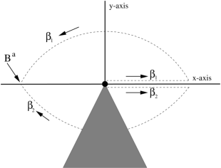
Figure 1: Space-time around a particle sitting at rest in the origin

If an observer approaches the point $B^{a}$ along path $\beta_{1}$ he will find coordinates:

$$B^{a}=\left(\begin{array}[]{ll}R\cos\varphi\\ R\sin\varphi\end{array}\right)$$ (14)

However, an observer moving along path $\beta_{2}$ would give point $B^{a}$ the coordinates:

$$B^{a}=\left(\begin{array}[]{ll}R\cos(\varphi+\alpha)\\ R\sin(\varphi+\alpha)\end{array}\right)$$ (15)

One observes that it is really the unusual ranges (or matching conditions) of the coordinates that make them multivalued. The main aim of this paper is to introduce new, single-valued, coordinates $(z,\bar{z})$, that transform the flat metric $\eta_{ab}$ into a nontrivial metric $g_{\alpha\beta}$ according to the well known transformation law:

$$g_{\mu\nu}=\partial_{\mu}u^{a}\partial_{\nu}u^{b}\eta_{ab}$$ (16)

Part of the gauge fixing-procedure is choosing a Cauchy-surface. The Cauchy surfaces we are looking for, are conveniently characterized by the property that they locally maximize the area of the surface. Since we know that locally there must always be a surface that has maximal area, we know that a solution to this coordinate condition always exists (i.e. the gauge is accessible). This is believed to be the simplest gauge condition that provides for single valued coordinates $(z,\bar{z},t)$, even though the elaboration of this condition is fairly complicated as will become clear. The coordinates $u^{a}(z,\bar{z};t)$ are considered as embedding conditions for each time t. They are flat coordinates but unfortunately multivalued functions on these Cauchy surfaces. So in order to descibe them we need cuts in the surface, called strings in previous literature. The transformation of $u^{a}$ over a string is in general a Poincaré transformation. We can also define the so called dreibein or tetrad fields on the surface $\Sigma$:

$$e_{\mu}^{~{}a}=\partial_{\mu}u^{a}$$ (17)

They are also multivalued but transform by homogeneous Lorenztransformations if we move over a string. In what follows we will often work in complex coordinates:

$$z = (x+iy)$$

$$\bar{z} = (x-iy)$$ (18)

It is easy to write down an action that would produce the slicing condition that the area of the Cauchy surface $\Sigma$ is locally maximal. We can view the coordinates $(z,\bar{z})$ as coordinates of a Euclidean worldsheet living in a flat 3 dimensional target-space described by the coordinates $u^{a}$. The embedding conditions for the worldsheet to have maximal area are then precisely given by the Polyakov action:

$$S_{p}=\int d^{2}z~{}\sqrt{\gamma}g^{ij}\partial_{i}u^{a}\partial_{j}u^{b}\eta_{ab}$$ (19)

where $g_{ij}$ is the 2 dimensional metric on the worldsheet, $\gamma=$det$g_{ij}$ and $\eta_{ab}$ is the 3 dimensional metric in the targetspace. We can also view the $g_{ij}$ as the induced metric on the Cauchy surface derived by projecting $\eta_{ab}$ on $\Sigma$. If we furthermore choose these coordinates on the worldsheet to be conformally flat:

$$g_{ij}=e^{\phi}\delta_{ij}$$ (20)

then this action reduces to:

$$S_{p}=\int d^{2}z~{}\partial u^{a}\bar{\partial}u^{b}\eta_{ab}$$ (21)

where we used the complex coordinates $(z,\bar{z}))$ and real coordinates $u^{a}$. Furthermore we used the notation: $\frac{\partial}{\partial z}=\partial~{}~{}\frac{\partial}{\partial\bar{z}}=\bar{\partial}$. It is well known that the equations that follow from the string action are:

$$\partial u^{a}\partial u^{b}\eta_{ab} = 0$$ (22)

$$\bar{\partial}u^{a}\bar{\partial}u^{b}\eta_{ab} = 0$$ (23)

$$\partial\bar{\partial}u^{a} = 0$$ (24)

This implies that $u^{a}$ is a harmonic function: $u^{a}(z,\bar{z};t)=u^{a}(z;t)+u^{a}(\bar{z};t)$. These conditions imply for the dreibein field (17):

$$e^{~{}a}_{0}\equiv\partial_{t}u^{a} = C^{a}(t)+\partial_{t}\int dz~{}e_{z}^{~{}a}+\partial_{t}\int d\bar{z}~{}e_{\bar{z}}^{~{}a}$$ (25)

$$e_{z}^{~{}a}\equiv\partial u^{a} = e_{z}^{~{}a}(z)~{}~{}~{}\mbox{(holomorphic)}$$ (26)

$$e_{\bar{z}}^{~{}a}\equiv\bar{\partial}u^{a} = e_{\bar{z}}^{~{}a}(\bar{z})~{}~{}~{}\mbox{(anti-holomorphic)}$$ (27)

$$e_{z}^{~{}a}e_{z}^{~{}b}\eta_{ab} = 0~{}~{}~{}~{}~{}~{}~{}~{}~{}~{}~{}\mbox{(null-vector)}$$ (28)

$$e_{\bar{z}}^{~{}a}e_{\bar{z}}^{~{}b}\eta_{ab} = 0~{}~{}~{}~{}~{}~{}~{}~{}~{}~{}~{}\mbox{(null-vector)}$$ (29)

where $C^{a}(t)$ is some vector only depending on t. Note that we still have a remaining conformal freedom: $z\rightarrow w(z)$. This will be used later to transform 2 particles to definit positions (leaving infinity invariant). Using equations (20),(12),(3) and (2) one can calculate what the implications are for the fields $g_{ij},\pi^{ij}$.

$$g_{ij} = e^{\phi}\delta_{ij}$$ (30)

$$\pi\equiv\pi^{l}_{l} = 0$$ (31)

The advantage of this gauge choice is now evident. First of all, as we will see later, we will only have to solve the holomorphic, null-vectorfields $e_{z}^{~{}a}$, living on the complex plane, in order to find the gravitational field $g_{\alpha\beta}$. The fact that the dreibein splits into a holomorphic and a anti-holomorphic part is a peculiar fact of 2+1 dimensional gravity. From a mathematical viewpoint it is a convenient gauge condition because we have now the machinery of complex calculus on Riemann surfaces at our disposal. The conformal freedom also suggests that there might be a connection with conformal field theory. As we will show later, the dreibein is formally solved as a two-point function of free conformal fermion fields with some twistoperator insertions. Another advantage is that in the reduction scheme explained in section 1, the reduced ”effective” Lagrangian looks very simple. Since $\pi$ is the canonicacally conjugate momentum of $2e^{\phi}$ and we have formulas (30) and (31) we find that in the Lagrangian (5) all kinetic terms of the gravitational field vanish: This is easily seen by splitting the kinetic term as follows:

$$\pi^{ij}\partial_{t}g_{ij}=(\pi^{T})^{ij}\partial_{t}g^{T}_{ij}+\pi\partial_{t}e^{\phi}$$ (32)

where $\pi\equiv\pi^{l}_{l}$ and a traceless tensor $P^{T}_{ij}$ is defined by

$$P^{T}_{ij}=P_{ij}-\frac{1}{2}P^{l}_{l}\delta_{ij}$$ (33)

So because $g^{T}_{ij}=0$ and $\pi=0$ we see that this kinetic term vanishes. Furthermore the term: $NH+N_{i}H^{i}$, which also contains matter contributions, must vanish because these are precisely the constraints that we solve. The reduced Lagrangian is thus given by the kinetic term of the matter fields and the surface term (13) which now only depends on the matter phase space variables because we (formally) solved the gravitational fields in terms of the matter variables. The surface term thus serves as a hamiltonian for the matter degrees of freedom. We will see later that it represents actually the total deficit angle of the universe (see [11]). As an example, we will work out the solution found in [2] for a massive, spinning particle at the origin, in our gauge. The solution for the metric will become degenerate near the particle. We are however not interested in that region since it is exactly the place where closed time-like curves may occur. At infinity this solution is however very interesting as we expect that any configuration of particles can be described asymptotically by an effective center of mass particle with mass M equal to the total energy contained in the universe and spin S equal to the total angular momentum of the universe. The solution therefore will provide the asymptotic behaviour of the gravitational fields.

If we use flat coordinates $u^{a}$ the matching conditions for this particle (sitting at rest in the origin) will be [2]:

$$\tilde{u}^{a} = R^{a}_{~{}b}u^{b}+q^{a}$$ (34)

$$R^{a}_{~{}b} = \left(\begin{array}[]{ccc}1&0&0\\ 0&\cos 2\pi\alpha&\sin 2\pi\alpha\\ 0&-\sin 2\pi\alpha&\cos 2\pi\alpha\\ \end{array}\right)$$ (38)

$$q^{a} = \left(\begin{array}[]{c}2\pi A\\ 0\\ 0\end{array}\right)$$ (42)

Here $\tilde{u}^{a}$ is the value of $u^{a}$ after an anti-clockwise rotation about the particle. Where we have defined: $\alpha=4GM$ and $A=4GS$. For a general choice of origin and a moving particle the identification will be an element of the Poincaré group:

$$\tilde{u}^{a}=(BRB^{-1})^{a}_{~{}b}u^{b}+q^{a}$$ (43)

Here $B^{a}_{~{}b}$ is a boost matrix with arbitrary rapidity $(\eta)$ and in an arbitrary direction, and $q^{a}$ is now a general translation (not necessarily of the form (42)). The line-element for the massive spinning particle sitting in the origin (not moving), found in [2], is given by:

$$ds^{2}=-(dt+Ad\theta)^{2}+\frac{1}{r^{2\alpha}}(dr^{2}+r^{2}d\theta^{2})$$ (44)

This is clearly not in the gauge we have chosen and to transform this into our gauge we have to write it as:

$$ds^{2}=-dt^{2}-2Adtd\theta(\rho,\omega)+e^{\phi}(d\rho^{2}+\rho^{2}d\omega^{2})$$ (45)

where the difference is in the $A^{2}d\theta^{2}$ term. We took here also $g_{oo}=-1$ because the system is stationary and $g_{oo}=\partial_{t}u^{a}\partial_{t}u^{b}\eta_{ab}$. The map from the $(t,r,\theta)$-coordinate system to the $(t,\rho,\omega)$-coordinate system is provided by:

$$\omega = \theta$$ (46)

$$\ln\frac{\rho}{\rho_{0}} = \frac{1}{1-\alpha}\mbox{arccosh}(\frac{r^{1-\alpha}}{A})|^{r}_{r_{0}}$$ (47)

If we choose ${r_{0}}^{1-\alpha}=A$ and $\rho_{0}=\rho(r_{0})=1$ and use the complex coordinates: $\rho=z\bar{z},\omega=\frac{1}{2i}\ln(\frac{z}{\bar{z}})$ we find for the line element in our gauge:

$$ds^{2}=-dt^{2}+\frac{iA}{z}dtdz-\frac{iA}{\bar{z}}d\bar{z}dt+\frac{A^{2}}{4z\bar{z}}[\frac{(z\bar{z})^{1-\alpha}}{A^{2}}-2+A^{2}(z\bar{z})^{\alpha-1}]dzd\bar{z}$$ (48)

So this will be the asymptotic behaviour of any metric describing N moving point-particles with total energy $\frac{\alpha}{4G}$ and total angular momentum $\frac{A}{4G}$. From here one finds that the coordinates $u^{a}$ are given by:

$$u^{0} = t+\frac{A}{2i}\ln z-\frac{A}{2i}\ln\bar{z}$$ (49)

$$u = \frac{1}{\sqrt{2}(1-\alpha)}[z^{1-\alpha}+\frac{A^{2}}{\bar{z}^{1-\alpha}}]$$ (50)

$$\bar{u} = \frac{1}{\sqrt{2}(1-\alpha)}[\bar{z}^{1-\alpha}+\frac{A^{2}}{z^{1-\alpha}}]$$ (51)

We see that both the $u^{0}$ and the $u$ and $\bar{u}$ are multivalued. Note that the log terms in $u^{0}$ are needed to generate the time jump of $8\pi GS$. The dreibein fields are given by:

$$\partial_{0}u^{a}=e_{0}^{a} = (1,0,0)$$ (52)

$$\partial_{z}u^{a}=e_{z}^{~{}a} = (\frac{A}{2iz},\frac{1}{\sqrt{2}z^{\alpha}},-\frac{A^{2}z^{\alpha-2}}{\sqrt{2}})$$ (53)

$$\partial_{\bar{z}}u^{a}=e_{\bar{z}}^{~{}a} = (-\frac{A}{2i\bar{z}},-\frac{A^{2}\bar{z}^{\alpha-2}}{\sqrt{2}},\frac{1}{\sqrt{2}\bar{z}^{\alpha}})$$ (54)

one can easily check that these dreibein fields fullfill our gauge conditions (26,27,28,29). These coordinates $u^{a}$ and the 3 dreibeins are only determined up to a global Lorentztransformation, since $\Lambda^{a}_{~{}b}u^{b}$ would produce the exact same line element (48). Actually we can choose our global Lorentzframe by the condition that the dreibeins have this asymptotic form. This immediately implies that the constant function $C^{a}(t)$ in (25) is determined to be $\delta^{a}_{0}$. In general however we will allow for more general global Lorentzframes (i.e. frames in which the center of mass moves). It will be this this global frame that determines the function $C^{a}(t)$.

3 the Riemann-Hilbert problem

The major advantage of our gauge choice is that the dreibein field splits into a holomorphic and a anti-holomorphic piece (and $e_{0}^{~{}a}$). In effect we only have to solve the $e_{z}^{~{}a}$-field because the $e_{\bar{z}}^{~{}a}$ is then given by:

$$e_{\bar{z}}^{~{}a}=F^{a}_{~{}b}(e^{~{}b}_{z})^{*}~{}~{}~{}~{}~{}F=\left(\begin{array}[]{ccc}1&0&0\\ 0&0&1\\ 0&1&0\end{array}\right)$$ (55)

Then, in the Lorentzframe where the effective center of mass is not moving, the $e_{0}^{~{}a}$-field is given by the the expression:

$$e_{0}^{~{}a}=\delta^{a}_{0}+\partial_{t}\int dz~{}e_{z}^{~{}a}+\partial_{t}\int d\bar{z}~{}e_{\bar{z}}^{~{}a}$$ (56)

So we only have to solve for the null-vector $e_{z}^{~{}a}$, living on the complex plane. We will not try to solve the Einstein-equations explicitly but we will use the monodromy properties of the dreibein. Now what happens if we parallel transport the dreibein $e_{z}^{~{}a}$ over a loop $\gamma_{n}$ around a point particle at position $a_{n}$. First we notice that we can deform the loop $\gamma_{n}$ as long as we don’t pass through a particle. This means that the tranformation will only differ on different homotopy classes of loops. To be more precise, we are interested in the transformations from the first homotopy class of loops on a punctured Riemann surface, to the group SO(2,1):

$$\pi_{1}(C-\{a_{1},...a_{N},\infty\};z_{o})\rightarrow\mbox{SO(2,1)}$$ (57)

$$[\gamma]_{n}\rightarrow M_{n}$$

We would like to view the coordinates $u^{a}(z)$ as multivalued functions on the complex plane. We therefore need a cut in the surface where the functions $u^{a}(z)$ transform. We attach to each particle a string over which the $u^{a}(z)$ transform as a Poincaré vector:

$$u^{a}\rightarrow(BRB^{-1}\cdot u)^{a}+l^{a}$$ (58)

At this point we should warn the reader that the translation vector $l^{a}$ is not the same as the translation vector $q^{a}$ in (43). This is due to the fact that we consider here only the holomorphic part of $u^{a}$. For the anti-holomorphic part we have a similar transformation with a translation vector $(l^{*})^{a}$. The correspondence is thus given by $q^{a}=l^{a}+(l^{*})^{a}$, which is a real vector. The transformation law (58) implies that the $e_{z}^{~{}a}=\partial u^{a}$ transform under the homogeneous part of the the Poincaré group; the Lorentzgroup. So if we parallel transport the dreibein along a closed curve (loop) $\gamma_{n}$ we find:

$$e_{z}^{~{}a}\stackrel{{\scriptstyle[\gamma]_{n}}}{{\rightarrow}}(B_{n}R_{n}B^{-1}_{n}\cdot e_{z})^{a}$$ (59)

As the particles evolve we don’t allow them to hit a string, so one cannot avoid that the strings might get ’knotted’ in a very complicated way.

Figure 2: Particles with strings attached moving on the complex plane.

On the other hand, if we have an expression for $e_{z}^{~{}a}$ we can reconstruct $u^{a}(z)$ by integrating once:

$$u^{a}(z)=\int dz~{}e_{z}^{~{}a}$$

It is now easy to see that the multivaluedness of $u^{a}(z)$ is indeed of the form (58). If we integrate around a singularity at $a_{i}$ we find:

$$\tilde{u}^{a}(z_{o}) = \int_{z_{o}}^{a_{k}}dz~{}e_{z}^{~{}a}+\oint_{a_{k}}dz~{}e_{z}^{~{}a}+M_{k}\int_{a_{k}}^{z_{o}}dz~{}e_{z}^{~{}a}$$ (60)

$$= (1-M_{k})A^{a}_{k}+\oint_{a_{k}}dz~{}e_{z}^{~{}a}$$ (61)

where $A^{a}_{i}\equiv\int_{z_{o}}^{a_{i}}dz~{}e_{z}^{~{}a}$ is the position of the particle in flat coordinates, and $M_{k}=B_{k}R_{k}B_{k}^{-1}$ (the monodromy matrix). Because $u(z_{o})=0$ is the origin of the flat coordinate system, the $\tilde{u}^{a}$ represent the shift of the origin and as such is equal to the vector $l^{a}$ of (58). If we integrate around 2 particles we find:

$$\tilde{u}^{a}(z_{o})=(1-M_{1})A^{a}_{1}+M_{1}(1-M_{2})A^{a}_{2}+\oint_{a_{1}}dz~{}e_{z}^{~{}a}+M^{a}_{1~{}b}\oint_{a_{2}}dz~{}e^{b}(z)$$ (62)

From this expression, together with the antiholomorphic part, we can derive the relative angular momentum of the 2 particles. It is defined in the center of mass frame of the 2 particles by:

$$L=[B^{-1}_{\rm c.o.m.}\cdot(l+l^{*})]^{0}$$ (63)

This is precisely the same expression as in [2] only if we demand:

$$\lim_{R\rightarrow 0}\oint_{a_{i}}dz~{}e_{z}^{~{}a}=0$$ (64)

where we take the radius $R$ of intgration to go to zero. To produce the multivaluedness of the $e_{z}^{~{}a}$ we expect, in the frame where the particle is boosted to rest, the following local behaviour near the location of a particle $a_{i}$:

$$(B^{-1}_{i}e_{z})^{a}\stackrel{{\scriptstyle z\rightarrow a_{i}}}{{\sim}}~{}z^{\lambda^{a}_{i}}H_{i}^{a}(z)$$ (65)

The $\lambda^{a}_{i}$ (called local exponents) are real numbers and the $H_{i}^{a}(z)$ are holomorphic functions near $a_{i}$. The condition (64) now implies that:

$$\lambda^{a}_{i}>-1$$ (66)

In fact we would like that for small $\alpha_{i}=4Gm_{i}$, the results do not differ much from the flat metric, i.e. the metric $g_{\mu\nu}$ is just slightly perturbed from the flat metric $\eta_{\mu\nu}$. This fact and the fact that $(B^{-1}e_{z})^{a}$ must produce a cut in the $z$-plane across which a vector must rotate over an angle $2\pi\alpha_{i}$ determines the local exponents to be:

$$\lambda^{a}_{i}=\left(\begin{array}[]{c}0\\ -\alpha_{i}\\ \alpha_{i}\end{array}\right)$$ (67)

See also [17]. Now we must take $\alpha_{i}\in~{}(0,1)$ in order to fullfill relation (66). Also if we would exceed this limit the total mass would become too large and the universe would close.
Note that if we would transform to a different global Lorentzframe, using a Lorentztransformation $\Lambda$, the effect on the monodromy would be

$$M_{n}\rightarrow\Lambda^{-1}M_{n}\Lambda$$ (68)

This is just a conjugation that doesn’t change the structure constants of the group (SO(2,1)). So the abstract group remains the same. Finally it is important to remark that if we follow a trajectory around all particles in the positive direction (anti-clockwise), this is equivalent to follow a trajectory around infinity in the negative direction, i.e.:

$$M_{tot}=B_{\infty}R^{-1}_{\infty}B^{-1}_{\infty}=B_{N}R_{N}B^{-1}_{N}.....B_{1}R_{1}B_{1}^{-1}$$ (69)

We will treat infinity as a singular point on the Riemann sphere, just as the particle positions. However because we demand that our universe is open the nature of this singularity will be slightly different from the particle singularities. We are now ready to reformulate our problem of solving the $e_{z}^{~{}a}$ as an old mathematical problem, the Riemann-Hilbert problem:
Given the following transformations for parallel transporting a vector around a closed loop:

$$e_{z}^{~{}a}\stackrel{{\scriptstyle[\gamma]_{n}}}{{\rightarrow}}M_{n~{}~{}b}^{~{}a}e_{z}^{~{}b}$$ (70)

$$[\gamma]_{n}\in\pi_{1}(C-\{a_{1},...a_{N},\infty\};z_{o})$$

$$M_{n}\in SO(2,1)$$

Find the multivalued, holomorphic (=meromorphic) functions $e_{z}^{~{}a}$ that transform in this way, with initial value $e^{~{}a}_{z}(z_{o})=\stackrel{{\scriptstyle o}}{{e}}_{z}^{~{}a}$.
It is actually more convenient to work in the locally isomorphic group SU(1,1). Denote $\zeta^{\alpha}(z)$ to be a spinor, transforming under SU(1,1) and $\zeta^{*\alpha}$ to be a spinor transforming under the complex conjugate representation of SU(1,1). (Note that $\zeta^{*\alpha}$ is not the complex conjugate of $\zeta^{\alpha}$.) If the components of $\zeta^{\alpha}$ are given by

$$\zeta^{\alpha}=\left(\begin{array}[]{c}a\\ b\end{array}\right)$$ (71)

then the spinor transforming under the complex conjugate representation is:

$$\zeta^{*\alpha}=\beta\left(\begin{array}[]{c}b\\ a\end{array}\right)$$ (72)

where $\beta$ is an arbitrary real constant. The vector $e_{z}^{~{}a}$ transforming under SO(2,1) is now constructed as follows:

$$e^{a}=\beta\left(\begin{array}[]{c}2ab\\ -i\sqrt{2}a^{2}\\ i\sqrt{2}b^{2}\end{array}\right)$$ (73)

Note that we automatically construct a null-vector $e_{z}^{~{}a}$ in this way. In the following we will always use this spinor representation SU(1,1) of the Lorentzgroup in 2+1 dimensions. The (modified) Riemann-Hilbert problem we have to solve is thus:

$$\zeta^{\alpha}\stackrel{{\scriptstyle[\gamma]_{n}}}{{\rightarrow}}M^{\alpha}_{n~{}\beta}\zeta^{\beta}$$ (75)

$$[\gamma]_{n}\in\pi_{1}(C-\{a_{1}...a_{N},\infty\},z_{o})$$

$$M_{n}\in SU(1,1)$$

The Riemann-Hilbert problem has a long and interesting history. Riemann was the first (1857) to work with a system of functions satisfying a linear differential equation with a given monodromy group (however, he couldn’t prove that this system of functions exists). In 1912 Hilbert added this problem to his list and since then many people worked on the problem (and solved it; that is, proved that there is a system of functions with a given monodromy group). People who worked on the problem were: Plemelj [12], Birkhoff, Röhrl (who proved the statement for an arbitrary Riemann surface) and Lappo-Danilevsky. Another important breakthrough was the reduction of the Riemann problem to a system of Schlesinger equations. For a review on this see [13, 14]. We will follow in this paper two important ways to solve the Riemann-Hilbert problem. First we will use a second order Fuchsian differential equation to attack the problem and solve the simple case of 2 particles. Then we will use the approach of a system of first order differential equations and the Schlesinger deformation equations to write down a general (formal) solution first found by Miwa, Sato and Jimbo [14].

3.1 The Fuchsian differential equation

It was already recognized by Riemann that differential equations with regular singularities have a monodromy group. If one would take the d independent solutions to the d’th order linear differential equation with N singular points (infinity is not included in the number N, but it is singular) and move them around a singular point they would transform into a linear combination of them. The general form of the differential equation with only regular singular points (i.e. Fuchsian singularities, see below) was found by Fuchs and reads:

$$\partial^{(d)}\zeta+\frac{P_{(N-1)}(z)}{Q(z)}\partial^{(d-1)}\zeta+\frac{P_{2(N-1)}}{Q^{2}(z)}\partial^{(d-2)}\zeta+....=0$$ (76)

$P_{l(N-1)}$ is a polynomial of order $l(N-1)$ and $Q=\prod^{N}_{k=1}(z-a_{k}).$
As we will use the 2 dimensional representation of the monodromy group SU(1,1) we can take d=2. If we had chosen to work with SO(2,1) we would have to take d=3. We want that the 2 independent solutions $\zeta^{1}$ and $\zeta^{2}$ to this equation are ”regular” singular near the points $a_{k}$. This implies that by definition they must have the following behaviour near $a_{k}$:

$$\zeta^{\alpha}=\stackrel{{\scriptstyle z\rightarrow a_{k}}}{{\sim}}(z-a_{k})^{\lambda^{\alpha}_{k}}[b^{\alpha}_{k}+c_{k}^{\alpha}(z-a_{k})+...]$$ (77)

This local behaviour is defined in a local basis where the monodromy is diagonal. In general the solution near a singular point is a linear combination of the 2 solutions ($\alpha=1,2$) given above (see (91)). The coeficients $\lambda^{\alpha}_{k}$ (called the local exponents) must obey the Fuchs relation:

$$\sum_{\alpha=1}^{d}\sum_{k=1}^{N}\lambda^{\alpha}_{k}+\sum_{\alpha=1}^{d}\lambda^{\alpha}_{\infty}=\frac{d(d-1)}{2}(N-1)$$ (78)

The first non-trivial case appears with 2 singularities (and infinity). This is also a special case because as we will explicitely show, the local exponents completely determine the Fuchsian differential equation and its solutions. With N singular points there will be (N-2) undetermined parameters (free parameters) in the differential equation. They must be determined by matching the monodromy matrices $M_{n}$ with the general monodromy of the solutions to that equation. If we have more than 2 singularities a complication is that apparent singularities may occur. (at most N-2 [13]). These are singular points in the differential equation but not in the solution. They will however generate zero’s in the $\zeta^{\alpha}$. At a zero the local exponents are possitive integers, and they are counted in the sum (78). This is reason why for more than 2 particles the method of finding a d’th order Fuchsian differential equation becomes very difficult and we use another method. Another remark is that the Riemann-Hilbert problem is not uniquely solvable if we only give the monodromy matrices. Let us define $\vec{\phi}(z)$ to be the d independent solutions to a definit Fuchsian differental equation. For a given monodromy there will exist d such sets of independent functions $\vec{\phi}_{i}(z)$, which are solutions to d Fuchsian differential equations with the same monodromy group but with different exponents at the singularities. These d sets are rationally independent with respect to eachother. I.e. a new set can always be written as:

$$\vec{f}(z)=\sum_{i=1}^{d}q_{i}(z)\cdot\vec{\phi}_{i}(z)$$ (79)

and $q_{i}(z)$ are rational functions. (rational functions will not change the monodromy of the solutions). A basic result is [15]:
Only if we specify the local exponents $\lambda^{\alpha}_{k}$ exactly (so not only up to an integer that would not change the monodromy, but also the integer part) then we can find a unique solution to the Riemann-Hilbert problem. As it turns out, the local exponents at $a_{k}$ are proportional to the masses of the particles and the local exponent at infinity to the total mass. As we saw in section 3, physics demands that we choose the masses in the range $(0,1)$. This determines the integer part of the exponents and makes the problem uniquely solvable. This method of finding a Fuchsian differential equation that has the right monodromy is particularly suited for the 2 particle case. We will use a different strategy for the general case. Below we will work out the 2 particle solution.

3.2 The 2 particle solution

To solve the 2 particle case one has to notice that a second order Fuchsian differential equation with 3 regular singularities, one of which is located at infinity, can always be written in the following form:

$$\partial^{2}\zeta+\sum^{2}_{k=1}\frac{1-\lambda^{1}_{k}-\lambda^{2}_{k}}{z-a_{k}}\partial\zeta+\{\sum^{2}_{k=1}\lambda^{1}_{k}\lambda^{2}_{k}\frac{(a_{k}-a_{k+1})}{z-a_{k}}+\lambda^{1}_{\infty}\lambda^{2}_{\infty}\}\cdot\frac{\zeta}{\prod_{i=1}^{2}(z-a_{i})}=0$$ (80)

where we have defined $a_{k}$ cyclic: $a_{3}=a_{1}$ etc. The general solution can be written symbolically using the Riemann-scheme:

$$\zeta=P\left\{\begin{array}[]{cccc}a_{1}&a_{2}&\infty&\\ \lambda^{1}_{1}&\lambda^{1}_{2}&\lambda^{1}_{\infty}&;z\\ \lambda^{2}_{1}&\lambda^{2}_{2}&\lambda^{2}_{\infty}&\end{array}\right\}$$ (81)

From this notation one can find in the upper row the singular points and in the second and third row the local exponents. Remember that these local exponents have to satisfy the Fuchs-relation:

$$\sum_{k,\alpha=1}^{2}\lambda^{\alpha}_{k}+\sum_{\alpha=1}^{2}\lambda^{\alpha}_{\infty}=1$$ (82)

Because we still had conformal freedom left in our gauge we can bring the points $\{a_{k}\}$ to respectively $\{0,1\}$ using the following conformal transformation:

$$w=\frac{(z-a_{1})}{(a_{2}-a_{1})}$$ (83)

We would like to transform this equation to the hypergeometric equation. This is possible by a transformation to a new variable $\xi(w)$, defined by:

$$\zeta(w)=w^{\lambda^{1}_{1}}(1-w)^{\lambda^{1}_{2}}\xi(w)$$ (84)

The Riemann-scheme now looks like:

$$\xi=P\left\{\begin{array}[]{cccc}0&1&\infty&\\ 0&0&\lambda^{1}_{1}+\lambda^{1}_{2}+\lambda^{1}_{\infty}&;w\\ \lambda^{2}_{1}-\lambda^{1}_{1}&\lambda^{2}_{2}-\lambda^{1}_{2}&\lambda^{1}_{1}+\lambda^{1}_{2}+\lambda^{2}_{\infty}&\end{array}\right\}$$ (85)

And this is precisely the Riemann-scheme for the hypergeometric function $F(a,b,c;w)$ with coeficients:

$$a = \lambda^{1}_{1}+\lambda^{1}_{2}+\lambda^{1}_{\infty}$$

$$b = \lambda^{1}_{1}+\lambda^{1}_{2}+\lambda^{2}_{\infty}$$

$$c = 1+\lambda^{1}_{1}-\lambda^{2}_{1}$$ (86)

There exist 2 independent solutions to the hypergeometric equation near $w=0$ (the series converges in the circle $|w|<1$):

$$\xi^{1} = F(a,b,c;w)$$ (87)

$$\xi^{2} = w^{1-c}F(1+a-c,b-c+1,2-c;w)$$ (88)

And also 2 rationally independent ones which one obtains by taking $\tilde{\lambda}^{1}_{\infty}=\lambda^{1}_{\infty}+1$ and $\tilde{\lambda}^{2}_{\infty}=\lambda^{2}_{\infty}-1$. We will however use the first ones, because they provide us with the right asymptotic behaviour. This means that the solution for $\zeta^{\alpha}$ around $w=0$ becomes (using some basic properties of F):

$$\zeta^{1} = w^{\lambda^{1}_{1}}(1-w)^{\lambda^{1}_{2}}F(a,b,c;w)$$ (89)

$$\zeta^{2} = w^{\lambda^{1}_{2}}(1-w)^{\lambda^{2}_{2}}F(1-a,1-b,2-c;w)$$ (90)

We will call this solution $\zeta^{\alpha}=(P(\lambda^{1}_{1}),P(\lambda^{2}_{1}))$. The argument of P determines the local exponent of that solution. If we want to find the solutions outside the circle $|w|=1$ we have to take the analytic continuation of this solution to the rest of the complex plane. Of course this is all well known for the hypergeometric equation. Denoting the 2 independent solutions to the Papperitz equations near $w=1$ and $w=\infty$ in the way as above we find that the analytic continuation looks like:

$$P(\lambda^{1}_{1}) = A^{1}_{2}P(\lambda^{1}_{2})+A^{2}_{2}P(\lambda^{2}_{2})$$

$$P(\lambda^{2}_{1}) = B^{1}_{2}P(\lambda^{1}_{2})+B^{2}_{2}P(\lambda^{2}_{2})$$

$$P(\lambda^{1}_{1}) = A^{1}_{\infty}P(\lambda^{1}_{\infty})+A^{2}_{\infty}P(\lambda^{2}_{\infty})$$

$$P(\lambda^{2}_{1}) = B^{1}_{\infty}P(\lambda^{1}_{\infty})+B^{2}_{\infty}P(\lambda^{2}_{\infty})$$ (91)

The coefficients can for instance be found in [16]. Using the local expansion (77) we can simply see what happens if we move around the location $a_{k}=\{0,1,\infty\}$. The $P(\lambda^{\alpha}_{k})$ will change as follows:

$$P(\lambda^{\alpha}_{k})\rightarrow e^{2\pi i\lambda^{\alpha}_{k}}P(\lambda^{\alpha}_{k})$$ (92)

we can actually derive the monodromy explicitely ([16]). In the following we will give these monodromy matrices and match them with the monodromy we impose for a particle. First we define the following basis:

$$u = R~{}\Lambda~{}P(\lambda^{1}_{1})$$ (93)

$$v = S~{}P(\lambda^{2}_{1})$$ (94)

Here R and S are functions of the parameters of the system only and $\Lambda$ is:

$$\Lambda = \frac{\Gamma(1+\lambda^{2}_{1}-\lambda^{1}_{1})\Gamma(\lambda^{1}_{1}+\lambda^{2}_{2}+\lambda^{1}_{\infty})\Gamma(\lambda^{1}_{1}+\lambda^{2}_{2}+\lambda^{2}_{\infty})}{\Gamma(1+\lambda^{1}_{1}-\lambda^{2}_{1})\Gamma(\lambda^{2}_{1}+\lambda^{2}_{2}+\lambda^{1}_{\infty})\Gamma(\lambda^{2}_{1}+\lambda^{2}_{2}+\lambda^{2}_{\infty})}$$ (95)

$$- \frac{\Gamma(1+\lambda^{2}_{1}-\lambda^{1}_{1})\Gamma(\lambda^{1}_{1}+\lambda^{1}_{2}+\lambda^{1}_{\infty})\Gamma(\lambda^{1}_{1}+\lambda^{1}_{2}+\lambda^{2}_{\infty})}{\Gamma(1+\lambda^{1}_{1}-\lambda^{2}_{1})\Gamma(\lambda^{2}_{1}+\lambda^{1}_{2}+\lambda^{1}_{\infty})\Gamma(\lambda^{2}_{1}+\lambda^{1}_{2}+\lambda^{2}_{\infty})}$$

Now the monodromy for moving around $w=0$ is:

$$M_{1}=\left(\begin{array}[]{cc}e^{2\pi i\lambda^{1}_{1}}&0\\ 0&e^{2\pi i\lambda^{2}_{1}}\end{array}\right)$$ (96)

And the monodromy for moving around $w=1$ is:

$$M_{2}=\left(\begin{array}[]{cc}\frac{\mu e^{2\pi i\lambda^{1}_{2}}-e^{2\pi i\lambda^{2}_{2}}}{\mu-1}&\frac{R}{S}(e^{2\pi i\lambda^{2}_{2}}-e^{2\pi i\lambda^{1}_{2}})\\ \mu\frac{S}{R}\frac{(e^{2\pi i\lambda^{1}_{2}}-e^{2\pi i\lambda^{2}_{2}})}{(\mu-1)^{2}}&\frac{\mu e^{2\pi i\lambda^{2}_{2}}-e^{2\pi i\lambda^{1}_{2}})}{\mu-1}\end{array}\right)$$ (97)

$$\mu=\frac{\sin\pi(\lambda^{1}_{1}+\lambda^{2}_{2}+\lambda^{2}_{\infty})\sin\pi(\lambda^{2}_{1}+\lambda^{1}_{2}+\lambda^{2}_{\infty})}{\sin\pi(\lambda^{2}_{1}+\lambda^{2}_{2}+\lambda^{2}_{\infty})\sin\pi(\lambda^{1}_{1}+\lambda^{1}_{2}+\lambda^{2}_{\infty})}$$ (98)

This monodromy has to be matched with the desired SU(1,1) monodromy. We will fix particle 1 (at $w=0$) and allow particle 2 (at $w=1$) to move in an arbitrary direction with an arbitrary velocity (see Fig. 3).

Figure 3: Two particles moving on the complex plane

The monodromy for particle 1 is then:

$$R_{1}=\left(\begin{array}[]{cc}e^{-i\pi\alpha_{1}}&0\\ 0&e^{i\pi\alpha_{1}}\end{array}\right)~{}~{}~{}~{}~{}~{}~{}~{}~{}\alpha_{i}=4Gm_{i}$$ (99)

The second particle has a more general monodromy of the form:

$$B_{2}R_{2}B_{2}^{-1}=\left(\begin{array}[]{cc}\cos(\pi\alpha_{2})-i\sin(\pi\alpha_{2})\cosh\eta&-\sin(\pi\alpha_{2})\sinh\eta e^{i\delta}\\ -\sin(\pi\alpha_{2})\sinh\eta e^{-i\delta}&\cos(\pi\alpha_{2})+i\sin(\pi\alpha_{2})\cosh\eta\end{array}\right)$$ (100)

The monodromy around $w=\infty$ is now fixed by the relation:

$$M_{1}M_{2}M_{\infty}=I$$ (101)

Matching the monodromies gives:

$$2\lambda^{1}_{1} = -\alpha_{1}~{}~{}~{}~{}\mbox{(mod $n_{1}$)}$$

$$2\lambda^{2}_{1} = \alpha_{1}~{}~{}~{}\mbox{(mod $n_{2}$)}$$

$$2\lambda^{1}_{2} = -\alpha_{2}~{}~{}~{}~{}\mbox{(mod $n_{3}$)}$$

$$2\lambda^{2}_{2} = \alpha_{2}~{}~{}~{}\mbox{(mod $n_{4}$)}$$ (102)

$$\mu = \coth^{2}(\frac{1}{2}\eta)$$ (103)

$$\frac{R}{S} = \frac{i}{2}\sinh\eta e^{i\delta}$$ (104)

We take here (mod $n_{i}$) $n_{i}\in Z$, instead of (mod $2n_{i}$). This has to do with the fact that SU(1,1) is the covering group of SO(2,1). In this case this implies both the transformations $\pm S\in$ SU(1,1) correspond to one element in SO(2,1). For reasons explained before (section 3) we will take $n_{i}=0$ (See also [17]). We can simplify relation (103) to:

$$\cos(2\pi\lambda^{2}_{\infty})=\cos(2\pi\lambda^{1}_{1})\cos(2\pi\lambda^{1}_{2})-\cosh\eta\sin(2\pi\lambda^{1}_{1})\sin(2\pi\lambda^{1}_{2})$$ (105)

This is the precisely the same relation found in [2]. We will therefore interpret $4\pi\lambda^{2}_{\infty}$ as the total deficit angle of the universe which means that $\alpha_{tot}\equiv 2\lambda^{2}_{\infty}$ must be in the range (0,1). Next we can use the Fuchs relation (82) to find $\lambda^{1}_{\infty}$:

$$\lambda^{1}_{\infty}=1-\lambda^{2}_{\infty}$$ (106)

The complex conjugate representation can be retrieved by using (72). Now we can write down the full solution to the monodromy problem:

$$\zeta^{\alpha}(w)=\beta\left(\begin{array}[]{l}\frac{i}{2}\sinh\eta e^{i\delta}\Lambda P(-\alpha_{1},\alpha_{2},\alpha_{tot};w)\\ P(\alpha_{1},\alpha_{2},\alpha_{tot};w)\end{array}\right)$$ (107)

with:

$$P(\alpha_{1},\alpha_{2},\alpha_{tot};w)=w^{\frac{\alpha_{1}}{2}}(1-w)^{\frac{\alpha_{2}}{2}}F(1+\frac{\alpha_{1}}{2}+\frac{\alpha_{2}}{2}-\frac{\alpha_{tot}}{2},\frac{\alpha_{1}}{2}+\frac{\alpha_{2}}{2}+\frac{\alpha_{tot}}{2},1+\alpha_{1};w)$$ (108)

Using the formula (73) we can write down the dreibein:

$$e_{z}^{~{}a}=\beta\left(\begin{array}[]{l}i\sinh\eta e^{i\delta}\Lambda P(\alpha_{1})P(-\alpha_{1})\\ \frac{i}{2\sqrt{2}}\sinh^{2}\eta e^{2i\delta}\Lambda^{2}P^{2}(-\alpha_{1})\\ i\sqrt{2}P^{2}(\alpha_{1})\end{array}\right)$$ (109)

It is now interesting to check the asymptotic behaviour found in formula (107). Since we know the local exponents at infinity we can write down the following expansion for $P(\lambda^{\alpha}_{\infty})$:

$$P(\lambda^{\alpha}_{\infty})=(\frac{1}{w})^{\lambda^{\alpha}_{\infty}}[b^{\alpha}_{\infty}+\frac{c^{\alpha}_{\infty}}{w}+.....]$$ (110)

with

$$\lambda^{1}_{\infty} = \frac{\alpha_{tot}}{2}$$ (111)

$$\lambda^{2}_{\infty} = 1-\frac{\alpha_{tot}}{2}$$ (112)

Using (73) we find the asymptotic behaviour for $e_{z}^{~{}a}$:

$$e_{z}^{~{}a}\stackrel{{\scriptstyle w\rightarrow\infty}}{{\sim}}\left(\begin{array}[]{l}w^{-1}\\ w^{-\alpha_{tot}}\\ w^{\alpha_{tot}-2}\end{array}\right)[B^{a}_{\infty}+\frac{C^{a}_{\infty}}{w}+.....]$$ (113)

It is important to realize that the global Lorentzframe we use to calculate the asymptotic behaviour is different from the one we used to calculate the $P(\lambda^{\alpha}_{1})$. In this frame particle 1 is not moving and as a result $M_{1}$ is diagonal in the basis $P(\lambda^{\alpha}_{1})$. In the frame we used to derive the asymptotic behaviour the monodromy around infinity is diagonal which means that the effective center of mass is not moving. The relation between the 2 frames is given by the coefficients $A^{\alpha}_{\infty}$ and $B^{\alpha}_{\infty}$ of (91). We see that the asymptotic behaviour is the same as in (52,53,54). One could also try to find the total angular momentum by matching the first coefficient in the expansion with (52,53,54):

$$B^{a}_{\infty}=(\frac{A}{2i},\frac{1}{\sqrt{2}},-\frac{A^{2}}{\sqrt{2}})$$ (114)

3.3 the N-body case

To treat the N-body case we will use a completely different approach, first followed by Schlesinger. Every monodromy problem will correspond to a first order matrix differential equation. First we write $\zeta^{\alpha}(z)=Y^{\alpha}_{~{}~{}\beta}\zeta^{\beta}(z_{o})$ where $Y(z)$ will be a fundamental matrix of solutions to the differential equation. The $Y(z)$ has the following properties:

1. $Y(z_{o})=I$

2. $Y(z)$ is holomorphic in $(C-\{a_{1}...a_{N},\infty\})$

3. $Y(z)$ has the following short distance behaviour near a singular point:

$$Y(z)\stackrel{{\scriptstyle z\rightarrow a_{i}}}{{\sim}}(z-a_{i})^{L_{i}}\hat{Y}_{i}(z)$$ (115)

where $M_{i}=e^{2\pi iL_{i}}$ and $M_{i}$ are the monodromy matrices. It is also important that the matrix $\hat{Y}_{i}(z)$ is holomorphic and invertable at $z=a_{i}$. So:

$$\hat{Y}_{i}(z)\stackrel{{\scriptstyle z\rightarrow a_{i}}}{{\sim}}(Y^{0}(a_{i})+Y^{1}(a_{i})(z-a_{i})+....)$$ (116)

with $\det|Y^{0}(a_{i})|\neq 0$.
To derive the form of the differential equation we first consider the object $Y^{-1}(\partial Y)$. This is also a single valued expression (the monodromy cancels out) and holomorphic at $(C-\{a_{1}...a_{N},\infty\})$. By using the local behaviour near the singularity $a_{i}$ we can find an expression near the location $a_{i}$:

$$Y^{-1}(\partial Y)\stackrel{{\scriptstyle z\rightarrow a_{i}}}{{\sim}}\hat{Y}^{-1}_{i}(z)\frac{L_{i}}{z-a_{i}}\hat{Y}_{i}(z)+\mbox{holomorphic at $z=a_{i}$}$$ (117)

Hence it must be of the form:

$$Y^{-1}(\partial Y)=\sum_{i=1}^{N}\frac{A_{i}}{z-a_{i}}$$ (118)

with

$$A_{i}=\mbox{Res}_{z\rightarrow a_{i}}Y^{-1}(\partial Y)=(Y^{0}_{i})^{-1}L_{i}Y^{0}_{i}$$ (119)

The behaviour of this equation at infinity can be studied by transforming to a new coordinate $w=\frac{1}{z}$. We find that that:

$$A_{\infty}=-\sum_{i=1}^{N}A_{i}$$ (120)

To prove that the solution to the differential equation:

$$\partial Y=\sum_{i=1}^{N}Y\frac{A_{i}}{z-a_{i}}$$ (121)

is unique we consider 2 solutions $Y_{1}$ and $Y_{2}$ and study the function $Y_{1}Y_{2}^{-1}$. Using the conditions ii) and iii) we see that this function is single valued and holomorphic everywhere on the Riemann sphere. This implies that it must be constant. Using i) we find that it must be actually $I$ and we have proved the statement: $Y_{1}=Y_{2}$, which in turn proves that the solution is unique. The proof that there actually exists a solution is much more involved and was only esthablished for the first time in its full generality by Röhrl. We will state the result obtained by Lappo-Danilevsky. He obtained a formal solution in terms of expansions in hyperlogarithms. See [13] for a review. He proved that if the $L_{i}$ were sufficiently small to ensure the convergence of this series, then the Riemann problem has d rationally independent solutions. Every other solution is given as a rational combination of these solutions. Remember that if we multiply $Y$ with a rational matrix $R(z)$ the monodromy does not change. Even when no convergence was guaranteed the solution could still be interpreted as analytic continuations. If we furthermore specify the local exponents exactly, that is specify the local behaviour of the spinor $\zeta^{\alpha}$ exactly (in a canonical basis), then we can find a unique solution for $\zeta^{\alpha}$ up to an overall constant. This constant must then be determined in our case by matching the series expansion of $e_{z}^{~{}a}$ at infinity with (53). An important additional condition is that the eigenvalues of $A_{1},...,A_{N},A_{\infty}$ (which are equal to the eigenvalues of $L_{1},...,L_{N},L_{\infty}$) do not differ by integers. In that case logarithmic singularities appear which we will not include in this paper. It was Miwa, Sato and Jimbo [14] who wrote down a solution to this monodromy problem in terms of correlators of free fermions with twistoperators at the positions of the singularities. It was Moore [18] who translated it in the language of a conformal field theory for free fermions. Their solution was:

$$Y^{\alpha}_{\beta}(z,z_{o},\{a_{i}\})=(z_{o}-z)\frac{\langle V_{\infty}(\infty)\psi^{\alpha}(z)\bar{\psi}_{\beta}(z_{o})V_{N}(a_{N})...V_{1}(a_{1})\rangle}{\langle V_{\infty}(\infty)V_{N}(a_{N})...V_{1}(a_{1})\rangle}$$ (122)

Figure 4: N Particles moving on the Riemann-sphere

The operators $V_{i}$ are twistoperators to be defined shortly (132). First of all, it is easily seen that taking the limit $z\rightarrow z_{o}$ we can write

$$Y^{\alpha}_{\beta}(z,z_{o},\{a_{i}\})=(z_{o}-z)\frac{\langle V_{\infty}(\infty)\overbrace{\psi^{\alpha}(z)\bar{\psi}_{\beta}(z_{o})}V_{N}(a_{N})...V_{1}(a_{1})\rangle}{\langle V_{\infty}(\infty)V_{N}(a_{N})...V_{1}(a_{1})\rangle}~{}$$ (123)

+ holomorphic terms at $z=z_{o}$
Where we have denoted the Wick-contraction as:

$$\overbrace{\psi^{\alpha}(z)\bar{\psi}_{\beta}(z_{o})}=-\frac{\delta^{\alpha}_{\beta}}{z-z_{o}}$$ (124)

Using the above formula we find that:

$$Y^{\alpha}_{\beta}(z_{o})=\delta^{\alpha}_{\beta}$$ (125)

as required by condition i). An important difference with [18] is that we have put a twistoperator at $z=\infty$, altering the ”outgoing vacuum” and changing the scaling dimensions of the fields at finite distances $a_{i}$. The twist at infinity must reproduce the monodromy at infinity and contains the information about the total mass of the universe.
We now come to the subject of choosing the twistoperators. They must be constructed in such a way that they reproduce the correct monodromy properties at $z=a_{i}$. In the following we will consider a particle at $z=0$ with boost-matrix $B_{i}=B$ and twistoperator $V_{i}(0)=V(0)$. We will drop the index i in the following. The same story holds for all the particles. For the particle at $z=0$ we want:

$$\psi^{\alpha}(e^{2\pi i}z)=M^{\alpha}_{~{}\beta}\psi^{\beta}(z)=(BRB^{-1})^{\alpha}_{~{}\beta}\psi^{\alpha}(z)$$ (126)

This means that the short distance behaviour of $\psi^{\alpha}(z)$ and $V(0)$ must be of the form:

$$V(0)\psi^{\alpha}(z)=\sum_{\beta}(B_{i})^{\alpha}_{~{}\beta}z^{D_{\beta}}H^{\beta}(z)$$ (127)

where B is a boost-matrix, $D_{\beta}$ are the eigenvalues of the matrix $L$ and $H^{\beta}$ is a holomorphic vector at $z=0$. We can write this as:

$$\sum_{\beta}B^{\alpha}_{\beta}z^{D_{\beta}}H^{\beta}=\sum_{\beta}(B\Omega(z))^{\alpha}_{\beta}H^{\beta}$$ (128)

where we supressed the index i and where:

$$\Omega(z)=\left(\begin{array}[]{cc}z^{-\frac{\alpha}{2}}&0\\ 0&z^{\frac{\alpha}{2}}\end{array}\right)~{}~{}~{}~{}~{}~{}~{}~{}~{}\alpha=4Gm$$ (129)

Due to $\Omega(z)$ this expression is multi-valued and, by analytic continuation, we find if we move around the particle at $z=a_{i}$:

$$(B\Omega(z))^{\alpha}_{~{}\beta}H^{\beta}\rightarrow(BRB^{-1})^{\alpha}_{~{}\beta}(B\Omega(z)H)^{\beta}$$ (130)

where:

$$R=\left(\begin{array}[]{cc}e^{-i\pi\alpha}&0\\ 0&e^{i\pi\alpha}\end{array}\right)$$ (131)

This is of course precisely the right monodromy and our task is to find the twistoprators with this property. In ref.[18] one finds:

$$V=:\exp[-p_{a}\int_{C}dw~{}\bar{\psi}_{\alpha}t_{\alpha\beta}^{a}\psi_{\beta}]:$$ (132)

where $:\bar{\psi}_{\alpha}(w)t^{a}_{\alpha\beta}\psi_{\beta}(w):\equiv J^{a}$ is the su(1,1) Kac-Moody current, and $C$ is a contour along the cut in the plane from the position $z=0$ to $\infty$, and $-p_{a}t^{a}_{\alpha\beta}=L_{\alpha\beta}$. In order to obtain the operator product expansion (OPE) at $z=0$ we note that we can use the freedom to transform the Dirac-spinors $\psi^{\alpha}$ by a global SU(1,1) transformation.

$$\psi^{\alpha}(z)\rightarrow\tilde{\psi}^{\alpha}=\Lambda^{\alpha}_{~{}\beta}\psi^{\beta}(z)$$ (133)

Next we write:

$$V(0)\psi^{\alpha}(z) = :\exp[\int_{C}dw~{}\bar{\psi}^{\mu}L_{\mu\nu}\psi^{\nu}]:\psi^{\alpha}(z)$$ (134)

$$= :\exp[\int_{C}dw~{}(\bar{\psi}B)^{\mu}(B^{-1}LB)_{\mu\nu}(B^{-1}\psi)^{\nu}]:\psi^{\alpha}(z)$$ (135)

Defining:

$$\tilde{\psi}^{\alpha} = (B^{-1}\psi)^{\alpha}$$ (136)

$$\tilde{\bar{\psi}}^{\alpha} = (\bar{\psi}B)^{\alpha}$$ (137)

we find:

$$V(0)\psi^{\alpha}(z)=:\exp[\int_{C}dw~{}\tilde{\bar{\psi}}^{\mu}D_{\mu\nu}\tilde{\psi}^{\nu}]:B^{\alpha}_{~{}\beta}\tilde{\psi}^{\beta}(z)$$ (138)

Here $D_{\mu\nu}=p_{0}t^{0}_{\mu\nu}=\frac{\alpha}{2}t^{0}_{\mu\nu}$, $\alpha=4Gm$ and $t^{0}_{\mu\nu}$=diag(1,-1).The next step is to bosonize the $\tilde{\psi}^{\alpha}$, $\tilde{\bar{\psi}}^{\alpha}$ and $\tilde{V(0)}~{}(=V(0))$. Of course we can not simultaneously diagonalize all the $L_{i}$, but we don’t need that actually because we only need the OPE locally at $z=0$. This result is independent of the representation that we choose (i.e. fermionic or bosonic). So we write:

$$\tilde{\psi}^{\alpha}(z) = :e^{i\varphi_{\alpha}(z)}:$$ (139)

$$\tilde{\bar{\psi}}(z) = :e^{-i\varphi_{\alpha}(z)}:$$ (140)

$$\sum_{\alpha}:\tilde{\bar{\psi}}^{\alpha}D_{\alpha}\tilde{\psi}^{\alpha}: = \sum_{\alpha}D_{\alpha}\partial\varphi_{\alpha}\equiv\vec{D}\cdot\partial\vec{\varphi}$$ (141)

$$\tilde{V}(0) = :e^{i\vec{D}\cdot\vec{\varphi}(0)}:$$ (142)

Where $D_{\alpha}$ are the eigenvalues of $L$. Formally we should add Klein-factors ($c_{\alpha}$ and $\bar{c}_{\alpha}$) to the expression $:e^{i\varphi_{\alpha}}:$ and $:e^{-i\varphi_{\alpha}}:$ to ensure that the fermions anticommute for all $\alpha$. We will leave them out in the following because we won’t need them futher. Note that if we bosonize the twistoperators (132) according to the rule (141), we also pick up a term at infinity: $V(0)=e^{i\vec{D}\cdot\vec{\varphi}(0)}e^{-i\vec{D}\cdot\vec{\varphi}(\infty)}$. This extra term is of course part of the twistoperator at infinity. There is thus a slight inconsistency in the notation. Because the twistoperators are really nonlocal operators they can not be assigned to 1 point.
Using the bosonic representation and the following identity:

$$:e^{i\vec{\kappa}\cdot\vec{\varphi}(z)}::e^{i\vec{\lambda}\cdot\vec{\varphi}(w)}:=(z-w)^{\vec{\kappa}\cdot\vec{\lambda}}:e^{i\vec{\kappa}\cdot\vec{\varphi}(z)+i\vec{\lambda}\cdot\vec{\varphi}(w)}:$$ (143)

we find for the OPE:

$$V(0)\psi^{\alpha}(z)=\sum_{\beta}B^{\alpha}_{~{}\beta}z^{D_{\beta}}H^{\beta}$$ (144)

where $H^{\beta}$ is again a holomorphic vector at $z=0$. This is precisely expression (127). So we esthablished the right behaviour of the solutions near the points $a_{i}$. The next question is obviously to check the behaviour of this solution at infinity. To find that one needs to know how the field $\psi^{\alpha}(z)$ scales, i.e. we need to know the scaling dimensions $\Delta^{\alpha}=2h^{\alpha}$ of the fermion. However the fact that we have put a twist operator at infinity spoils the naive scaling dimensions (see [19]). Before we do that we like to get rid of the $z_{o}$ dependence. More precisely we want to replace condition i) in the beginning of this section by a different condition at $z=\infty$. That new condition is:

• $$\hat{Y}^{0}_{\infty}=I$$ (145)

To implement this new condition we first have to bring the field $\bar{\psi}_{\beta}(z_{o})$ to infinity, using the rule:

$$\bar{\psi}_{\beta}(\infty)=\lim_{z_{o}\rightarrow\infty}\bar{\psi}_{\beta}(z_{o})z_{o}^{\Delta_{\beta}}~{}~{}~{}~{}~{}~{}~{}\Delta_{\beta}=1$$ (146)

In front of expression (122) we have a factor $(z_{o}-z)$ and we use this factor ($(z_{o}-z)\sim z_{o}$ if $z_{o}\rightarrow\infty$) to take the limit (146). However there is already a twistoperator at infinity which implies that we will have to deal with another divergent factor. For convenience we will assume that the center of mass is not moving, which means that at infinity the monodromy is diagonal. The twist at infinity is defined by the total action of the twists at finite points. Because all these twists contain integrals from the particle position $a_{i}$ to infinity, and at infinity all these twists do not add up to zero, there is a nontrivial twist at infinity, see Fig. 4.
To see what happens if we bring the operator $\bar{\psi}_{\beta}(z_{o})$ close to this twistoperator we first bring $V_{\infty}$ to a point $b$ in the finite plane and bosonize:

$$V_{\infty}(b)\bar{\psi}_{\beta}(z_{o})=:e^{-i\vec{D}_{\infty}\cdot\vec{\varphi}(b)}::e^{-i\varphi_{\beta}(z_{o})}:\sim(b-z_{o})^{D_{\beta}^{\infty}}H_{\beta}(z)$$ (147)

where $H_{\beta}(z)$ is holomorphic at $z=b$. This suggests that if we want to take the limit $z_{o}\rightarrow b$ we have to do the following:

$$\lim_{z_{o}\rightarrow b}(b-z_{o})^{-D^{\infty}_{\beta}}V_{\infty}(b)\bar{\psi}_{\beta}(z_{o})=:V_{\infty}(b)\bar{\psi}_{\beta}(b):$$ (148)

One can check that if we take the limit:

$$\lim_{z_{o}\rightarrow b}(b-z_{o})^{-D_{\beta}^{\infty}}Y^{\alpha}_{~{}\beta}$$ (149)

we have precisely the condition i’) at z=b:

$$\hat{Y}^{0}_{b}=I$$ (150)

This means that in taking the fermion $\bar{\psi}_{\beta}(z_{o})$ to infinity we need to multiply by a factor $z_{o}^{D_{\beta}}$ in order to obey the new condition i’) at infinity. All together we write now:

$$Y^{\prime\alpha}_{~{}\beta}=\lim_{z_{o}\rightarrow\infty}z_{o}^{D^{\infty}_{\beta}}Y_{~{}\beta}^{\alpha}=\frac{\langle:V_{\infty}\bar{\psi}_{\beta}:\psi^{\alpha}(z)V_{N}...V_{1}\rangle}{\langle V_{\infty}V_{N}...V_{1}\rangle}$$ (151)

To determine the asymptotic behaviour of $Y^{\prime}$ we have to calculate the scaling behaviour of the $\psi^{\alpha}(z)$. To do that we again bosonize and note once more that we have chosen the center of mass to be at rest, meaning that $V_{\infty}$ has a ”diagonal form”. As mentioned before, the operator $:V_{\infty}\bar{\psi}_{\beta}:$ at infinity spoils the naive scaling behaviour. In the bosonized picture we have the following operator at infinity:

$$O^{\infty}_{\beta}=:e^{-i\vec{D}_{\infty}\cdot\vec{\varphi}-i\varphi_{\beta}}:$$ (152)

Following ([19]) we must change the scaling dimensions by the following rule:

$$\Delta^{\prime\alpha}=1-(D^{\infty}_{\alpha}+\delta^{\alpha}_{\beta})$$ (153)

This means that the asymptotic behaviour of $Y^{\prime}$ looks like:

$$\left(\begin{array}[]{cc}z^{-\frac{\alpha_{tot}}{2}}H_{11}(z)&z^{-\frac{\alpha_{tot}}{2}-1}H_{12}(z)\\ z^{\frac{\alpha_{tot}}{2}-1}H_{21}(z)&z^{\frac{\alpha_{tot}}{2}}H_{22}(z)\end{array}\right)$$ (154)

where $H_{ij}(z)$ are holomorphic functions as $z\rightarrow\infty$. Next we choose $\stackrel{{\scriptstyle o}}{{\zeta}}^{\alpha}=(1,0)$ so that we have:

$$\zeta^{\alpha}\stackrel{{\scriptstyle z\rightarrow\infty}}{{\sim}}\left(\begin{array}[]{c}z^{-\frac{\alpha_{tot}}{2}}\\ z^{\frac{\alpha_{tot}}{2}-1}\end{array}\right)[b_{\infty}^{\alpha}+c_{\infty}^{\alpha}\frac{1}{z}+...]$$ (155)

This is in fact the right asymptotic behaviour at $z\rightarrow\infty$. One can actually find an explicit expression for these correlators in ([14]). This is a rather formal infinite series and hardly of any practical use to us. Therefore we will not repeat it here. The first order matrix differential equation can be viewed as an equation for parallel transport on a Riemann-sphere. We can define a connection:

$${\cal A}=\sum_{i}\frac{A_{i}}{z-a_{i}}$$ (156)

and a covariant derivative

$${\cal D}=\frac{\partial}{\partial z}-{\cal A}$$ (157)

In this picture $e_{z}^{~{}a}$ is determined by parallel transporting the $e^{\alpha}(z_{o})$ from $z_{o}$ to $z$. The result depends on the path we choose. Because the connection ${\cal A}$ is holomorphic everywhere except at the singularities $a_{i}$ and $\infty$ the result will only depend on the first homotopy class of the punctured sphere. In general the dependence of the $A_{i}$ on the points $a_{i}$ can be very difficult. If we use normalisation condition i) then also a dependence on $z_{o}$ is possible. Schlesinger determined a differential equation for this dependence by demanding that if we move the particles to another location (for instance by time-evolution!) the monodromy will not change. This is because we don’t allow the particles to cross a string connected to one of the other particles, by smoothly deforming the string to another position as a particle comes close to a string. This also means that the topology of the strings will become very important in the dynamics of the particles. Another way of putting the fact that the monodromy does not change during time-evolution is that the flat momenta $p_{a}$ are conserved. They act as a kind of charges in this picture. The equations found by Schlesinger are called isomonodromic deformation equations and are given with the normalisation i’) by:

$$\frac{\partial Y^{\prime}}{\partial a_{i}} = -\frac{A_{i}}{z-a_{i}}Y^{\prime}$$ (158)

$$\frac{\partial A_{i}}{\partial a_{j}} = \frac{[A_{j},A_{i}]}{a_{j}-a_{i}}~{}~{}~{}~{}~{}~{}~{}~{}~{}~{}~{}~{}~{}i\neq j$$ (159)

$$\frac{\partial A_{i}}{\partial a_{i}} = -\sum_{k\neq i}\frac{[A_{k},A_{i}]}{a_{k}-a_{i}}$$ (160)

In order to get a feeling for the solution presented in (122) we will calculate a simple example, namely the case where all $A_{i}$ commute. From (158,159,160) we see that the $A_{i}$ do not depend on the particle’s positions $a_{i}$. Next we diagonalise all $A_{i}$ simultaneously. This means that we are describing a static configuration of particles. It is very easy to find the exact solution to the differential equation (121):

$$Y=\prod_{i=1}^{N}(\frac{z-a_{i}}{z_{o}-a_{i}})^{D_{i}}$$ (161)

where :

$$D_{i}=\left(\begin{array}[]{cc}\frac{-\alpha_{i}}{2}&0\\ 0&\frac{\alpha_{i}}{2}\end{array}\right)~{}~{}~{}~{}~{}~{}~{}\alpha_{i}=4Gm_{i}$$ (162)

The answer in the normalisation i’) is according to (151):

$$Y^{\prime}=\lim_{z_{o}\rightarrow\infty}z_{o}^{D_{\infty}}Y=\prod_{i=1}^{N}(z-a_{i})^{D_{i}}$$ (163)

In the static case it is indeed true that $M_{tot}=\sum_{i=1}^{N}m_{i}$. Next we choose the vector $\stackrel{{\scriptstyle o}}{{\zeta}}^{\alpha}=(1,0)$ so that we find:

$$\zeta^{\alpha}=(\prod_{i=1}^{N}(z-a_{i})^{-\frac{\alpha_{i}}{2}},0)$$ (164)

and

$$e_{z}^{~{}a}=(0,\prod_{i=1}^{N}(z-a_{i})^{-\alpha_{i}},0)$$ (165)

Now using the formula (55) we can calculate the conformal factor defined by $e^{\phi}=e^{a}_{z}(z)e_{\bar{z},a}(\bar{z})$ (see (20)):

$$e^{\phi}=\prod_{i=1}^{N}(z-a_{i})(\bar{z}-\bar{a_{i}})^{-\alpha_{i}}$$ (166)

which is the correct answer (see [2]) On the other hand we would like to calculate the correlator (151). Because all $L_{i}$ commute we can bosonize the fermions at all points $a_{i}$ simulteneously. We may view the fermion $\psi^{\alpha}(z)$ as two twistoperators with ”charge” $1$ and $\bar{\psi}_{\beta}(z_{o})$ as 2 twistoperators with ”charge” $-1$. The correlators that we have to calculate ($\alpha,\beta=1,2$) are only nonzero if the total charge adds up to $\alpha_{tot}$. This is due to the infrared cut-off that has to be taken care off [19]. Only when the total charge is $\alpha_{tot}$ we find a nonzero correlator. Now using repeatedly formula (143) and noticing that only for $\alpha=\beta$ the total charge adds up to $\alpha_{tot}$ we find:

$$Y^{\prime}=\frac{\prod_{i=1}^{N}(z-a_{i})^{D_{i}}\prod_{i<j}^{N}(a_{i}-a_{j})^{\vec{D_{i}}\cdot\vec{D_{j}}}}{\prod_{i<j}^{N}(a_{i}-a_{j})^{\vec{D_{i}}\cdot\vec{D_{j}}}}=\prod_{i=1}^{N}(z-a_{i})^{D_{i}}$$ (167)

The use of the operators at infinity is now to ensure that the total charge adds up to $\alpha_{tot}$:

$$\sum_{i=1}^{N}\alpha_{i}=\alpha_{tot}~{}~{}~{}~{}~{}~{}~{}~{}~{}~{}~{}~{}~{}\alpha=\beta$$ (168)

We could call this a Coulomb-gas picture since it bears much resemblance with the background Coulomb-gas of ref.[19]. Finally we want to say something about the correlator: $\langle V_{\infty}V_{N}...V_{1}\rangle$. We can derive a kind of Knizhnik-Zamalodchikov equation for this correlator (see also [18]). For that consider first:

$$\frac{\frac{1}{2}\langle V_{\infty}[\bar{\psi}_{\beta}(z_{o})\frac{\partial}{\partial z}\psi^{\alpha}(z)-\frac{\partial}{\partial z_{o}}\bar{\psi}_{\beta}(z_{o})\psi^{\alpha}(z)]V_{N}...V_{1}\rangle}{\langle V_{\infty}V_{N}...V_{1}\rangle}$$ (169)

$$=-\frac{\delta^{\alpha}_{\beta}}{(z_{o}-z)^{2}}+\frac{\langle V_{\infty}\tilde{T}^{\alpha}_{\beta}V_{N}...V_{1}\rangle}{\langle V_{\infty}V_{N}...V_{1}\rangle}$$ (170)

where we have defined:

$$\tilde{T}_{\beta\alpha}\equiv:\frac{1}{2}\bar{\psi}_{\beta}(z_{o})\frac{\partial}{\partial z_{o}}\psi_{\alpha}(z_{o})-\frac{1}{2}\frac{\partial}{\partial z_{o}}\bar{\psi}_{\beta}(z_{o})\psi_{\alpha}(z_{o}):$$ (171)

Because we have a background charge at infinity, the naive ”energy-momentum tensor” $\tilde{T}\equiv tr\tilde{T}$ has to be corrected by a boundary term:

$$T=\tilde{T}-\sum_{\alpha}\frac{1}{2}D^{\infty}_{\alpha}\partial:\bar{\psi}_{\alpha}\psi_{\alpha}:$$ (172)

The boundary term however does not change the simple pole term in the OPE so that we still have:

$$L_{-1}=\oint_{a_{i}}dz\frac{T(z)}{2\pi i}=\oint_{a_{i}}dz\frac{\tilde{T}(z)}{2\pi i}=\frac{\partial}{\partial a_{i}}$$ (173)

So we find:

$$\oint_{a_{i}}\frac{\langle V_{\infty}\tilde{T}V_{N}...V_{1}\rangle}{2\pi i\langle V_{\infty}V_{N}...V_{1}\rangle}=\frac{1}{\langle V_{\infty}V_{N}...V_{1}\rangle}\frac{\partial}{\partial a_{i}}{\langle V_{\infty}V_{N}...V_{1}\rangle}$$ (174)

On the other hand we may also write the correlator as:

$$\frac{\frac{1}{2}\langle V_{\infty}[\bar{\psi}_{\beta}(z_{o})\frac{\partial}{\partial z}\psi^{\alpha}(z)-\frac{\partial}{\partial\bar{z}}\bar{\psi}_{\beta}(z_{o})\psi^{\alpha}(z)]V_{N}...V_{1}\rangle}{\langle V_{\infty}V_{N}...V_{1}\rangle}=-\frac{1}{2}\frac{\partial}{\partial z}\frac{Y_{\alpha\beta}}{z_{o}-z}+\frac{1}{2}\frac{\partial}{\partial z_{o}}\frac{Y_{\alpha\beta}}{z_{o}-z}$$ (175)

This can be worked out by using an expansion around $z_{o}$:

$$Y=I+{\cal A}(z_{o})(z-z_{o})+\frac{1}{2}[\frac{\partial}{\partial z_{o}}{\cal A}(z_{o})+{\cal A}^{2}(z_{o})](z-z_{o})^{2}$$ (176)

${\cal A}$ is defined in (156). Integrating this expression around $z_{o}=a_{i}$ and comparing with (174) we get:

$$\frac{\partial}{\partial a_{i}}{\langle V_{\infty}V_{N}...V_{1}\rangle}=\frac{1}{2}\oint_{a_{i}}dz_{o}~{}~{}\sum_{i,j}\frac{tr~{}A_{i}A_{j}}{(z_{o}-a_{i})(z_{o}-a_{j})}$$ (177)

As mentioned before there also exists a Schlesinger equation in which $z_{o}$ is included in the set deformation parameters (see [14]). The equation we need is:

$$\frac{\partial A_{i}}{\partial z_{o}}=\sum_{j}\frac{[A_{i},A_{j}]}{z_{o}-a_{j}}$$ (178)

We can use this formula to find that $tr~{}A_{i}A_{j}$ does not depend on $z_{o}$ at all! This allows us to calculate the integral in (177) and we finally find:

$$\frac{\partial}{\partial a_{i}}{\langle V_{\infty}V_{N}...V_{1}\rangle}=\frac{1}{2}\sum_{i\neq j}\frac{tr~{}A_{i}A_{j}}{a_{i}-a_{j}}{\langle V_{\infty}V_{N}...V_{1}\rangle}$$ (179)

Although this looks a bit like a Knizhnik-Zamalodchikov equation, there is are differences. Most importantly, the term $tr~{}A_{i}A_{j}$ may depend in a very complicated way on the positions of the particles $a_{i}$. The fact that we didn’t find a Knizhnik-Zamalodchikov-equation (with constant matrices $A_{i}$) is interpreted in [21] as a result of the fact that on the Cauchy-surface the translational symmetry is broken.
As solving the Riemann-Hilbert problem is equivalent to finding the $A_{i}$, we have in general not an explicit expression for them. Only in some special cases, where we are able to find the $A_{i}$ we can write down a full solution to the Riemann-Hilbert problem. It is also very interesting to look at the OPE of 2 twistoperators and determine the monodromy if one particle moves around the other. Alternatively one can look at the exchange-algebra (or half-monodromy) and determine what happens if 2 particles are exchanged. We expect that these half-monodromies obey some non-abelian representation of the Yang-Baxter equation (see [20]). We hope to say more about this in the future.

4 Discussion

In a series of papers [2, 3] ’t Hooft solved the classical N-particle problem in 2+1 dimensional gravity. In his approach he used flat coordinates $u^{a}$ that obey unusual boundary conditions. As a result these coordinates become multivalued. In this polygon approach he developed a Hamiltonian formulation for the phase space variables and by replacing Poisson-Brackets by commutators he was able to formulate a first quantized theory. It is however rather difficult to write down an explicit wave function in this formalism as all kinds of transitions that could take place have to be taken into account as boundary conditions on the wave functions. Surely if one wants to formulate a second quantized theory these boundary conditions become untractable. This was the main motivation for us to define a single-valued coordinate system, much like in the case of anyons where one has multi-valued and single-valued gauges. In the case of anyons the single-valuedness has a price, namely the introduction of an electromagnetic interaction between the anyons. Also in the case of 2+1 dimensional gravity we can trade the multivaluedness for a nontrivial gravitational interaction. This implies that we have to introduce a nontrivial metric $g_{\mu\nu}\neq\eta_{\mu\nu}$.

The physical quantities of the theory are the particle positions and the conjugate momenta. As the gravitational field doesn’t have any degrees of freedom it is in principle possible to integrate them out. To do that one must first study the gravitational field in our particular gauge. That is precisely what we did in this article and we found that the 2 particle case could be solved explicitly while in the N-particle case, the gravitational field (or rather the dreibeins) could be represented in terms of correlators of a two dimensional conformal field theory.

In order to reduce the system to its physical degrees of freedom we need to find a Hamiltonian. In section 1 it was argued that the Hamiltonian is given by a boundary term:

$$H=\int d^{2}x~{}~{}\sqrt{h}~{}^{(2)}R=\oint dz~{}\partial\phi(z\bar{z})~{}~{}+~{}~{}\oint d\bar{z}~{}\bar{\partial}\phi(z,\bar{z}).$$ (180)

where $\phi$ is defined by: $e^{\phi}=e^{a}_{z}(z)e_{\bar{z},a}(\bar{z})$. This expression can be simply evaluated by using the monodromy-matrix at infinity and the asymptotic behaviour of $\phi(z,\bar{z})$ (48). One finds the expected result; $H=\alpha_{tot}$, the total deficit angle of the universe. By using (69) it then easy to find the well known result:

$$-2\pi iH~{}t^{o}_{\alpha\beta}=\log[\prod_{i=1}^{N}e^{2\pi iL_{i}}]_{\alpha\beta}$$ (181)

where $L_{i}=-p^{i}_{a}t^{a}_{\alpha\beta}$ ; $p_{a}^{(i)}$ are the flat momenta and $t^{a}_{\alpha\beta}$ are the generators of SO(2,1) (or equivalently SU(1,1)). Because we restricted ourselves in this paper to particles with positive mass, and didn’t consider anti-particles with negative mass (which could in principle be defined) we have positive total energy. It is however also particular simple in our gauge to prove that for arbitrary matter couplings (that obey reasonable boundary conditions at infinity) the total energy of an open universe is positive definit (see [9, 11]). This is of course a nessecary property in order to have stable vacuum in a second quantized theory. It is also important to realise that gravity in 2+1 dimensions contains long range interactions. This can be seen most easily in the flat coordinate-system because the wedge cut out of space-time extends out to infinity. This means that we don’t have an asymptotic flat region. If we want to define an S-matrix in the future we know that we will have to define in- and out-states with great care. We hope to say more about the particle dynamics and the quantisation of this system in the future.

Note added

While writing this paper I found out that A. Bellini et al. [17] published a preprint concerning the same issues we adress.

References

- [1] Misner C W, Thorne K S and Wheeler J A 1973 Gravitation (San Francisco: W.H. Freeman and Company)
- [2] Deser S, Jackiw R and ’t Hooft G 1984 Ann. Phys. 152 220
-
[3]
’t Hooft G 1992 Class. Quant. Grav. 9 1335
’t Hooft G 1993 Class. Quant. Grav. 10 S79
’t Hooft G 1993 Class. Quant. Grav. 10 1023
’t Hooft G 1993 Class. Quant. Grav. 10 1653 - [4] Witten E 1988 Nucl. Phys. B331 46
-
[5]
Grinani G and Nardelli G 1992 Phys. Rev. D45 2719
Vaz C and Witten L 1992 Nucl. Phys. B368 509
Vaz C and Witten L 1992 Mod. Phys. Lett. A7 2763 - [6] Carlip S 1993 Canadian Gen. Rel. 1993 215
-
[7]
’t Hooft G 1988 Comm. Math. Phys. 117 685
Deser S and Jackiw R. 1988 Comm. Math. Phys. 118 495 -
[8]
Carlip S 1989 Nucl. Phys. B324 106
Koehler K, Mansouri, Vaz C and Witten L 1991 Nucl. Phys B348 373 - [9] Ashtekar A and Varadarajan M 1994 Phys. Rev. D50 4944
- [10] Regge T and Teitelboim C 1974 Ann. Phys. 88 286
- [11] Henneaux M 1984 Phys. Rev. D29 2766
- [12] Plemelj J 1964 Problems in the sense of Riemann and Klein (London: John Wiley)
-
[13]
Chudnovsky D V 1979 in Bifurcation phenomena in
mathematical physics and related topics Bardos C and Bessis P (eds.) pp. 385
(Dordrecht: D. Reidel Publishing Company)
Chudnovsky G V 1979 in Complex Analysis, Microcalculus, and Relastivistic Quantum Theory Lagolnitzer D (ed.) Lecture notes in physics 120 (New York: Berlin Springer Verlag) - [14] Sato M, Miwa T and Jimbo M 1979 in Complex Analysis, Microcalculus, and Relastivistic Quantum Theory Lagolnitzer D (ed.) Lecture notes in physics 120 (New York: Berlin Springer Verlag)
- [15] Blok B and Yankielowicz S 1989 Nucl. Phys. B321 717
- [16] Sansone G. and Gerretsen 1969 Lectures on the theory of functions of a complex variable II (Groningen: Wolters- Noordhoff)
-
[17]
Bellini A, Ciafaloni M and Valtancoli 1995 (2+1)-Gravity
with
moving particles in an instantaneous gauge Preprint: CERN-TH/95-192
Bellini A, Ciafaloni M and Valtancoli 1995 Non-perturbative particle dynamics in (2+1)-gravity Preprint CERN-TH/95-193 - [18] Moore G 1990 Comm. Math. Phys. 133 261
- [19] Dotsenko V S and Fattev V A 1984 Nucl. Phys. B240 312
- [20] Verlinde E 1990 Bombay Quant. Field Theory 1990 450
- [21] Ferrari F 1993 Comm. Math. Phys. 156 179