Thermodynamics of $N=1$ supersymmetric QCD

USITP-95-09

October-1995

hep-th/9510045

J. Grundberg^†, T.H. Hansson^⋆ and U. Lindström^⋆

ABSTRACT

We use the dual description proposed by Seiberg to calculate the pressure in the low temperature confined phase of $N=1$ supersymmetric QCD using perturbation theory to $O(g^{3}_{m})$, where $g_{m}$ is the gauge coupling in the dual theory. Combining this result with the usual high temperature expansion based on asymptotic freedom, we study how the physics in the intermediate temperature regime depends on the relative size of the scale parameters in the two descriptions. In particular we explore the possibility of having a temperature range where both perturbation expansions are valid.

^†Department of Mathematics and Physics, Mälardalens högskola,
Box 833, S-721 23 Västerås, Sweden
^⋆Fysikum, University of Stockholm, Box 6730, S-11385 Stockholm, Sweden
^⋆ Supported by the Swedish Natural Science Research Council (NFR).

1. Introduction

A standard method to investigate the phase diagram for a theory at finite temperature is to use high-temperature and low-temperature expansions of the free energy: At each temperature one calculates the free energy by using the variables appropriate at that temperature. In QCD, asymptotic freedom tells us that the high $T$ expansion can be done in perturbation theory and that the relevant degrees of freedom are quarks and gluons. At low temperature, however, the theory becomes strongly coupled, confinement sets in and other variables have to be used. The low $T$ degrees of freedom are the hadrons, and one calculates the low $T$ expansion using a phenomenological description of a gas of the lightest hadrons, i.e. the pions.

Recently, there has been a break-through in the understanding of the infrared structure of certain 4D supersymmetric Yang-Mills theories. The strongest results are for $N=2$ SUSY [3], where the low-energy effective action can be calculated exactly, but there are also very interesting results for $N=1$ [4, 5]. (For an introduction and a list of references see [6]). In particular, Seiberg has argued that there often exists two dual descriptions of the same theory, one ”electric” and one ”magnetic”. As in usual electric-magnetic duality in the presence of monopoles, strong coupling in one description implies weak coupling in the other, and a ”fundamental” field in one description can appear as a soliton in the other.

In the models considered by Seiberg, the duality between weak and strong coupling is manifested in a rather surprising way: Both descriptions are SUSY gauge theories, with the same global $SU(N_{f})$ flavour symmetry, but with different gauge symmetry. In the case of an $SU(N_{c})$ color symmetry in the electric theory, the magnetic gauge group is $SU(N_{f}-N_{c})$. Since the beta function is $\sim(3N_{c}-N_{f})$, the theories are asymptotically free (UVF) or infrared free (IRF) depending on the value of $N_{f}$. For $N_{f}<\frac{3}{2}N_{c}$, the electric theory is UVF and the magnetic IRF. For $N_{f}>3N_{c}$, the reverse holds, and for $\frac{3}{2}N_{c}<N_{f}<3N_{c}$, they are both UVF. Seiberg’s duality conjecture, which is supported by several very strong consistency checks, asserts that the two theories are identical in the infrared. Furthermore, stability of the ground state imposes the condition $N_{f}\geq N_{c}$, and it turns out the the cases $N_{f}=N_{c}$ and $N_{f}=N_{c}+1$ are special [4]. In the following we shall restrict $N_{f}$ to be larger than $N_{c}+1$. If the gauge group of the electric theory is $SO(N)$, the magnetic theory has gauge group $SO(N_{f}-N_{c}+4)$ and we shall consider the intervals $N_{c}<N_{f}<3(N_{c}-2)/2$ and $N_{c}>4$, or $N_{f}=N_{c}>5$, where again the magnetic theory is IRF. It is of interest to study both the $SU(N)$ and the $SO(N)$ case since we expect a phase transition from a low temperature confined phase to a high temperature deconfined phase for $SO(N)$. In the $SU(N)$ case, no deconfining phase transition is expected since there is matter in the fundamental representation that will give a perimeter behaviour to the Wilson loop even at zero temperature (or, equivalently, a non zero value to the Polyakov loop).

The main idea of this paper is to exploit the duality in the range $N_{c}+1<N_{f}<\frac{3}{2}N_{c}$ (for $SU(N)$) to calculate the leading contributions to the pressure in the electric theory both at high and low $T$. Since this theory is UVF we have the standard perturbative high $T$ expansion, but at low energy we can now invoke duality and use perturbation theory in the IRF magnetic theory.

In the next section we outline the calculation of the pressure both at low and high temperature while referring some details to an Appendix. In section 3 we discuss the range of validity of the expansions and to what extent perturbation theory can be used to obtain information about the finite $T$ phase structure. In particular we discuss the importance of the scale parameters that control the electric and magnetic coupling constants in the asymptotic regions of large and high temperature respectively.

2. Calculations

In superfield notation [7, 8] the action for SUSY QCD is given by,

$$S=\frac{1}{4}\int d^{4}x\,d^{2}\,\theta Tr(W^{\alpha}W_{\alpha})+h.c.+\int d^{4}xd^{4}\theta[(\bar{\phi}_{i}\phi_{i})+(\tilde{\bar{\phi}}_{i}\tilde{\phi}_{i})]$$ (1)

where $W^{\alpha}=W^{\alpha A}T^{A}$ is the $SU(N_{c})$ gauge field strength and the covariantly chiral matter superfields $\phi^{a}_{i}$ transform according to the $\bf N_{c}$ representation of the gauge group ($a=1,...,N_{c}$ is the $SU(N_{c})$ index, $i=1,..,N_{f}$ is the flavour index). The covariantly chiral superfields $\tilde{\phi}_{ai}$ transform according to the $\bf\overline{N_{c}}$ representation. Both $\phi$ and $\tilde{\phi}$ are needed to get a non-chiral theory. In terms of ordinary fields the theory contains $N_{g}=N_{c}^{2}-1$ gluons ($A_{\mu}^{A}$), and gluinos, ($\lambda^{\alpha A}$, $\bar{\lambda}^{\dot{\alpha}A}$), $A=1,..,N_{g}$, and also $N_{c}N_{f}$ quarks ($\psi_{\alpha a}$, $\bar{\psi}_{\dot{\alpha}}^{a}$, $\tilde{\psi}^{\alpha b}$, $\bar{\tilde{\psi}}^{\dot{\alpha}}_{b}$) and squarks ($\varphi_{a}$, $\varphi^{\star}_{a}$, $\tilde{\varphi}^{a}$, $\tilde{\varphi}^{\star a}$), $a=1,...,N_{c}$. The flavour indices on quarks and squarks are suppressed. For $SO(N)$, the number of gluons is $N_{g}=N_{c}(N_{c}-1)/2$, and the matter fields are in a real representation.

Greens functions in SUSY theories are usually calculated using supergraph techniques [7, 8]. At finite temperature, bosons and fermions do not enter the calculation on equal footing, and it is better to use a component formalism. In the Appendix we define our conventions, and give the component form of the Lagrangian that give the Feynman rules shown in figs. 6 - 9.

We can now use the standard machinery of finite temperature field theory to calculate the free energy density ${\cal F}=-P$ at temperature $T$. The calculations in a theory with zero masses and chemical potentials are very straightforward, as demonstrated by an example in the Appendix.

To $O(g^{0})$ the pressure is due to the ”blackbody” radiation from the massless degrees of freedom. For SUSY QCD with gauge group $SU(N_{c})$, the bosonic degrees of freedom are the $2N_{g}$ gluons and the $4N_{c}N_{f}$ squarks. There is an equal number of fermionic partners to these (gluinos and quarks), and thus the ”blackbody” part of the pressure is given by

$${\it P}_{0}^{el} = (2N_{g}+4N_{c}N_{f})\left(1+\frac{7}{8}\right)\frac{\pi^{2}T^{4}}{90}$$ (2)

$$= (N_{c}^{2}+2N_{c}N_{f}-1)\frac{\pi^{2}T^{4}}{24}\ \ \ \ \ .$$

To get the corresponding result for $SO(N)$, one substitutes the value for $N_{g}$ given above and also replaces $N_{f}$ by $N_{f}/2$ since quarks and squarks are in real representations and thus contribute only half as many degrees of fredom as in the $SU(N)$ case. In the dual magnetic description the gauge group is replaced by $SU(N_{f}-N_{c})$ but the number of flavours remains $N_{f}$. Following Seibergs duality hypothesis, we also need $N_{f}\times N_{f}$ free chiral multiplets, which for $SU(N)$adds $2N_{f}^{2}$ bosonic degrees of freedom (and an equal number fermionic ones), and thus for the dual ”magnetic” description we get

$${\it P}_{0}^{mag} = \left[2[(N_{f}-N_{c})^{2}-1)]+4(N_{f}-N_{c})N_{f}+2N_{f}^{2}\right]\left(1+\frac{7}{8}\right)\frac{\pi^{2}T^{4}}{90}$$ (3)

$$= P_{0}^{el}+4N_{f}\left(N_{f}-\frac{3N_{c}}{2}\right)\frac{\pi^{2}T^{4}}{24}\ \ \ \ \ .$$

For SO(N) we have a similar expression remembering that the gauge group is now $SO(N_{f}-N_{c}+4)$ and that the meson multiplet is formed from a symmetric combination of two complex fields, and thus has $2\,N_{f}(N_{f}+1)/2$ components.

Comparing (2) and (3), we see that if $N_{f}<3N_{c}/2$ the number of ”blackbody” degrees of freedom in the electric description is greater than the corresponding number in the magnetic description. This is a reasonable result: The same condition $N_{f}<3N_{c}/2$ describes the the range of $N_{f}$ for which the magnetic description is infrared free and the electric theory is confining. (We remind the reader that in the region $3N_{c}/2<N_{f}<3N_{c}$ Seiberg has argued that we should have a non-abelian Coulomb phase and that the electric theory loses asymptotic freedom at the upper of these limits.) We would certainly expect the number of massless ”hadrons” to be smaller than the number of constituents in a confining theory, and this is exactly what we find. A similar calculation for the case of $SO(N_{c})$, where the limiting case is when $N_{f}=3(N_{c}-2)/2$, gives the same result: The number of massles degrees of freedom in the electric theory is larger than the ones in the dual magnetic theory as long as the electric theory is confining and the magnetic is infrared free.

Figure 1: Some of the $g^{2}$-contributions

The $O(g^{2})$ contribution to the pressure is obtained by calculating diagrams of the type shown in fig. 1, using the rules given in the Appendix. The result is

$$P_{2}^{el}=-N_{g}\left(C_{A}+3T_{f}\right)\frac{g^{2}T^{4}}{64}\ \ \ \ \ ,$$ (4)

where $C_{A}$ is the Casimir operator for the adjoint representation, and $T_{f}$ depends on the matter content. For $SU(N)$, $C_{A}=N_{c}$ and $T_{f}=N_{f}$, while for $SO(N)$, $C_{A}=(N_{c}-2)/2$ and $T_{f}=N_{f}/2$. The pressure in the magnetic theory is obtained by replacing $N_{c}$ by $N_{f}-N_{c}$ or $N_{f}-N_{c}+4$ for $SU(N)$ and $SO(N)$ respectively. (Note that the region we consider, the extra chiral fields are non-interacting, so they contribute only to the blackbody pressure.)

In theories with massless bosons, the next contribution is $O(g^{3})$, rather than $O(g^{4})$, due to the infrared singularities related to the ring diagrams exemplified in fig. 2. The techniques for calculating these diagrams are well known, and essentially amonts to calculating the (thermal) electric mass, $m_{el}$, for the gluons and the thermal mass, $m_{sq}$, for the squarks. These masses are readily obtained from the standard self-energy diagrams, and we find,

$$m_{el}^{2} = \frac{1}{2}(C_{A}+T_{f})\,g^{2}T^{2}$$ (5)

$$m_{sq}^{2} = \frac{N_{g}}{12N_{c}}\,g^{2}T^{2}\ \ \ \ \ .$$

This implies the following result for the $O(g^{3})$ contribution to the pressure,

$${\it P}_{3}^{el}=\left[\left(\frac{C_{A}+T_{f}}{2}\right)^{3/2}N_{g}+2\left(\frac{N_{g}}{12N_{c}}\right)^{3/2}N_{c}T_{f}\right]\frac{g^{3}T^{4}}{12\pi}\ \ \ \ \ ,$$ (6)

$(\frac{N_{c}}{3}+\frac{N_{f}}{6})^{3/2}N_{g}$, and again the result in the corresponding magnetic theory is obtained by replacing $N_{c}$ by $N_{f}-N_{c}$, or by $N_{f}-N_{c}+4$.

Figure 2: Ring-diagrams

To get the total pressure to $O(g^{3})$ in the electric theory we add ${\it P}^{el}_{0}$, ${\it P}^{el}_{2}$ and ${\it P}^{el}_{3}$ and replace $g^{2}$ by a runing coupling constant at temperature T,

$$g^{2}_{el}=\frac{8\pi^{2}}{b_{el}\ln(T/\Lambda_{el})}$$ (7)

and for the magnetic theory we add the corresponding results and replace $g^{2}$ by

$$g^{2}_{mag}=\frac{4\pi^{2}}{b_{mag}\ln(\Lambda_{mag}/T)}$$ (8)

For $SU(N)$, $b_{el}=3N_{c}-N_{f}$ and $b_{mag}=N_{f}-3N_{c}/2$, while for $SO(N)$, $b_{el}=3N_{c}/2-N_{f}/2-3$ and $b_{mag}=3N_{c}/2-3-N_{f}$. The expression for $g^{2}_{el}$ is valid for $T\gg\Lambda_{el}$ and the one for $g^{2}_{mag}$ for $T\ll\Lambda_{mag}$. If we define the ratio $x=\Lambda_{mag}/\Lambda_{el}$, there is a possibility of using perturbation theory in both the electric and magnetic theory simultaneously if $1<T/\Lambda_{el}<x$. This will be discussed further below. Finally we should stress a very important point: Because of supersymmetry, the vacuum energy is identically zero, and thus also the pressure at zero temperature. This is not the case for non-supersymmetric theories like QCD, where there is a non-zero vacuum pressure (related to the quark an gluon condensates, and phenomenologically manifested by the so called bag constant) that is important for understanding the finite $T$ phase transitions [2].

3. Discussion

We shall first discuss the validity of the high and low T expressions for the pressure derived in the previous section. It is known that in QCD, the perturbative expansion of the ($T=0$ subtracted) free energy is well defined only to $O(g^{5})$, since at $O(g^{6})$ it becomes sensitive to the non-perturbatively generated $O(g^{2})$ magnetic mass. For a good discussion of the results to $O(g^{3})$ see [2]. Recently the $O(g^{4})$ term in pure Yang-Mills theory has been calculated by Arnold and Zahi [10]. The conclusion, so far, is that perturbation theory is reliable only at very high temperatures, and this is likely to be true also for the theories we are considering here. Unfortunately, because of finite size corrections, not even the most recent lattice simulations of pure YM theory are good enough to really settle how well perturbation theory works. For theories with dynamical fermions, like the one studied here, we may have to wait long before reliable lattice results are available. Another point which is relevant for this discussion is the contribution to the pressure from topologically nontrivial gauge configurations. In particular, for QCD the contributions from instantons have been calculated by Pisarski and Yaffe (for a review see [11]) who showed that the instantons become important only at temperatures too low for perturbation theory to be valid. It would be interesting to repeat this calculation in the supersymmetric case.

The presence of two scale parameters, $\Lambda_{el}$ and $\Lambda_{mag}$, requires some comment. $\Lambda_{el}$ is the usual renormalization group invariant scale of the asymptotically free (electric) gauge theory, and just as in ordinary QCD it sets the scale for the onset of nonperturbative phenomena. While less familiar, the situation is very similar in an IR free theory. The reason that this is not always stressed in the prototype IR free theory, QED, is that the electron mass provides a natural renormalization point. Since $\alpha$ is very small at this scale, nonperturbative effects become important only at distances so short that QED must be extended to the full electroweak theory. If, however, the electron had been massless, using a running coupling constant and a renormalization group invariant scale would be as natural in QED as in QCD. Again the renormalization group invariant scale parameter $\Lambda_{QED}$ would tell us at what scale the non-perturbative (short distance) physics becomes important.

In the theories we consider, naturalness implies that there is only one scale connected to the onset of nonperturbative phenomena. However, this does not mean that the $\Lambda$ parameter occuring in the UV (or electric) or IR (or magnetic) description of the theory are necessarily the same. The $\Lambda$-parameters depends on the renormalization scheme and could well be different. In our case $g_{el}$ becomes large as $T$ approaches $\Lambda_{el}$ from above, and $g_{mag}$ becomes large as $T$ approaches $\Lambda_{mag}$ from below. Thus there are two possibilities: 1) $\Lambda_{mag}\leq\Lambda_{el}$. In this case the temperature region in between $\Lambda_{mag}$ and $\Lambda_{el}$ is not even in principle accessible in perturbation theory. 2) $\Lambda_{mag}>\Lambda_{el}$. Here there is a $\em possibility$ of simultaneously using perturbation theory in both the electric and the magnetic description, but there is of course no guarantee, or even great hope, that the perturbative expansions will be good in the overlap region. At present we have no way of determining which of these alternatives is correct - this could only be settled by matching a direct nonperturbative calcualtion in the electric theory, e.g. using lattice methods, to a corresponding weak coupling calculation in the magnetic theory. Any concrete idea for how to perform such a calculation would be very desireable.

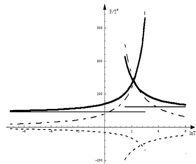
Figure 3: Pressure versus logaritm of the temperature for $N_{c}=9$, $N_{f}=12$, $\Lambda_{el}=1$ and $\Lambda_{mag}=x\Lambda_{el}=50\Lambda_{el}$. The thin solid lines are the blackbody contributions, the dotted lines the $O(g^{2})$, the dashed lines the $O(g^{3})$ and the thick lines the total contributions.

Clearly, the second of the above alternatives is the more interesting one, and we shall now investigate it a bit further. In fig. 3 we show the $SU(N)$ $O(g^{0})$, $O(g^{2})$ and $O(g^{3})$ contributions to the pressure as a function of $\ln(T/\Lambda_{el})$ for $x=\Lambda_{mag}/\Lambda_{el}=50$. We see that even though the ratio $x$ is taken (presumably unrealistically) large perturbation theory looks very poor in the overlap region. The reason is the large coefficients in front of the logarithms in the $O(g^{2})$ and $O(g^{3})$ terms. One might have hoped to see a qualitative difference between the the $SU(N)$ and $SO(N)$, since a phase transition in expected for the latter, but in fact fig. 3 is typical for both gauge groups.

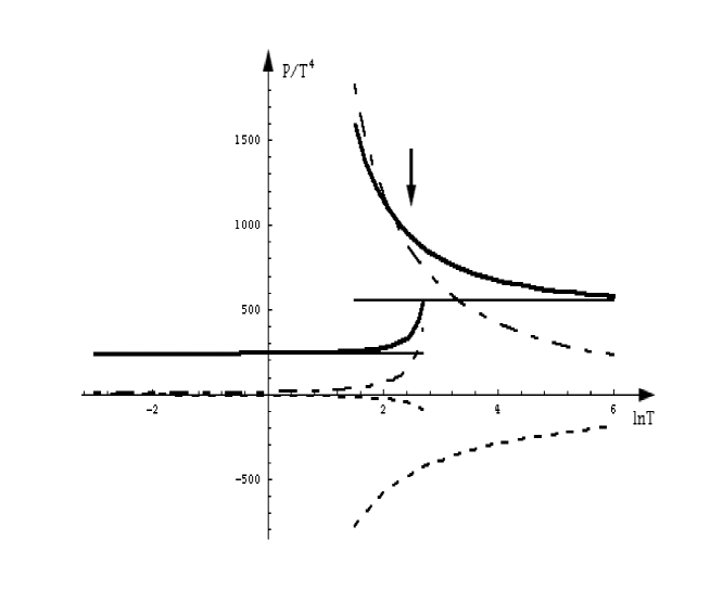
Figure 4: Pressure versus logaritm of the temperature for $N_{c}=N_{f}=30$, $\Lambda_{el}=1$ and $\Lambda_{mag}=x\Lambda_{el}=20\Lambda_{el}$. The lines have the same meaning as in fig. 3.

An obvious question is whether there is a range of parameters $N_{c}$ and $N_{f}$ where the coefficents of the logarithms become small. The answer is yes, by simply noting that for $N_{f}$ very close to $N_{c}$ the number of magnetic gluons is small and thus also the coupling in the magnetic theory. This is most clearly seen in the large $N_{c}$ limit where the $O(g^{2})$ and $O(g^{3})$ corrections vanish for $N_{f}/N_{c}\rightarrow 1$. In fig. 4 we show the different components of the pressure in the $SO(N)$ case, where a phase transition in expected, for $N_{c}=N_{f}=30$ and $x=20$. In this, admittedly rather extreme case, it is not unreasonable to assume that both perturbation expansions can be trusted in the region in the proximity of the arrow. The shape of the curves are however not compatible with having a phase transition, where the pressure must be continuous, and concavity of the free energy density requires that discontinuities of the derivative of the pressure, and hence of $P/T^{4}$, must be such that it increases with $T$. From this we can conclude that the value $x=20$ cannot be correct, so the perturbative analysis have in fact allowed us to put a bound on the intrinsically non-perturbative parameter $\Lambda_{mag}/\Lambda_{el}$. Also note, that a bound on $x$ also translates into a bound on $T_{c}/\Lambda_{el}$, where $T_{c}$ is the transition temperature. Clearly these bounds are not very strict, and we have not made any attempts to systematically explore different values for $x$, $N_{f}$ and $N_{c}$.

In conclusion, we have explored the possibility of using perturbation theory to study both the high and low temperature regime in N=1 SUSY theories possessing Seiberg duality. First we noted that the number of black-body degrees of freedom in the electric theory is larger than in the magnetic, exactly in the region where the former is UV freee and the second IR free, which is what is naively expected in a confining theory. We calculated the pressure to $O(g^{3})$ in both the UV and IR regime, and discussed various possibilities for the intermediate temperature regime. Our results are somewhat disappointing, in the sense that the dream of finding a regime where both perturbation expansions were applicable was not fullfilled. We did, however, manage to glean some nonperturbative information from our calculations by studying the large $N_{c}$ limit.

There are several directions in which this work might be extended that could be of interest. We have already mentioned that instanton effects could change our resulsts, and so could of course higher order terms in perturbation theory. Another interesting question is to study the deformed theories, either by including mass terms, or by breaking the global symmetries by choosing moduli parameters different from zero. In particular one could ask whether finite temperature effects would induce a flow in moduli space, and thus making some vacuua unstable against bubble formation.

Acknowledgements: We thank A. Fayyazuddin, and P. Di Vecchia for discussions and N. Seiberg for a useful correspondence.

Appendix A. Feynman rules

In components, the lagrangian density (1) takes the form,

$${\cal L}=-\frac{1}{4}F^{A\mu\nu}F^{A}_{\mu\nu}+i\lambda^{\alpha A}(D\bar{\lambda})_{\alpha A}+i{\tilde{\psi}}^{\alpha a}(D\bar{\tilde{\psi}})_{\alpha a}-i\bar{\psi}^{\dot{\alpha}a}(D\psi)_{\dot{\alpha}a}$$

$$+(D^{\mu}\varphi)^{+a}(D_{\mu}\varphi)_{a}+(\tilde{D}^{\mu}\tilde{\varphi})^{a}(\tilde{D}_{\mu}\tilde{\varphi})^{+}_{a}$$

$$+i\sqrt{2}g\left[(\varphi^{\star}T^{A}\psi^{\alpha})\lambda_{\alpha}^{A}+(\bar{\psi}^{\dot{\alpha}}T^{A}\varphi)\bar{\lambda}^{A}_{\dot{\alpha}}+\lambda^{A}_{\alpha}(\tilde{\psi}^{\alpha}T^{A}\tilde{\varphi}^{\star})+(\tilde{\varphi}T^{A}\bar{\tilde{\psi}}_{\dot{\alpha}})\bar{\lambda}^{\dot{\alpha}A}\right]$$

$$-\frac{1}{2}g^{2}\sum_{a}\left[(\varphi^{\star}T^{A}\varphi)-(\tilde{\varphi}T^{A}\tilde{\varphi}^{\star})\right]^{2}$$ (A.1)

where the matrices $T^{A}$, $A=1...N_{g}$ span the fundamental representation of $SU(N_{c})$, and where we have suppressed contractions of group indices. The various covariant derivatives are defined as follows:

$$(D\bar{\lambda})_{\alpha A} = (\sigma^{\mu})_{\alpha\dot{\alpha}}[\partial_{\mu}\delta_{AB}+gf_{ABC}A^{C}_{\mu}]\lambda^{b}$$

$$(D\psi)^{\dot{\alpha}}_{a} = (\bar{\sigma}^{\mu})^{\dot{\alpha}\alpha}[\partial_{\mu}\delta_{a}^{b}+igA^{A}_{\mu}(T^{A})_{a}^{b}]\psi_{\alpha b}$$

$$(D\bar{\tilde{\psi}})_{\alpha a} = (\sigma^{\mu})_{\alpha\dot{\alpha}}[\partial_{\mu}\delta_{a}^{b}+igA^{A}_{\mu}(T^{A})_{a}^{b}]\bar{\tilde{\psi}}^{\dot{\alpha}}_{b}$$

$$(D_{\mu}\varphi)_{a} = [\partial_{\mu}\delta_{a}^{b}+igA^{A}_{\mu}(T^{A})^{b}_{a}]\varphi_{b}$$

$$(D_{\mu}\varphi)^{+a} = \partial_{\mu}\varphi^{\star a}-ig\varphi^{\star b}(T^{A})_{b}^{r}A_{\mu}^{A}$$

$$(\tilde{D}_{\mu}\tilde{\varphi})^{a} = \partial_{\mu}\tilde{\varphi}^{a}-ig\tilde{\varphi}^{b}(T^{A})_{b}^{r}A^{A}_{\mu}$$

$$(\tilde{D}_{\mu}\tilde{\varphi})^{+}_{a} = [\partial_{\mu}\delta^{b}_{a}+igA^{A}_{\mu}(T^{A})_{a}^{b}]\tilde{\varphi}^{\star}_{b}$$ (A.2)

Our Minkowski metric is $\eta_{\mu\nu}=diag(1,-1,-1,-1)$, and the $2\times 2$-matrices $\sigma^{\mu}$ and $\bar{\sigma}^{\mu}$ satisfy the relations

$$\sigma^{\mu}_{\alpha\dot{\alpha}}\bar{\sigma}^{\nu\dot{\alpha}\beta}+\sigma^{\nu}_{\alpha\dot{\alpha}}\bar{\sigma}^{\mu\dot{\alpha}\beta}=2\eta^{\mu\nu}\delta_{\alpha}^{\beta}$$

$$\bar{\sigma}^{\mu\dot{\alpha}\alpha}\sigma^{\nu}_{\alpha\dot{\beta}}+\bar{\sigma}^{\nu\dot{\alpha}\alpha}\sigma^{\mu}_{\alpha\dot{\beta}}=2\eta^{\mu\nu}\delta^{\dot{\alpha}}_{\dot{\beta}}$$ (A.3)

From the action we read off the Feynman rules given in figs. 6 - 9. For the gauge group $SO(N)$ the rules are identical except that since the matter multiplets are real, there are no dotted quark or squark lines. In the calculations, this only amounts to an overall factor of 2 for the relevant diagrams.

B. Sample Calculation

We illustrate the calculation of the $g^{2}$ contributions by evaluating the diagram in fig. 6 involving one gluon and two gluinos.

Figure 5: Diagram contributing to the pressure to $O(g^{2})$.

Using the Feynman rules and dropping a temperature independent piece[2] we find,

$${\cal I}_{Ggg} = -{\textstyle{1\over 2}}g^{2}\int_{-}dpdq\int_{+}dk\left\{{\left({{i(\bar{\sigma}p)^{\dot{\beta}\beta}\delta^{C\bar{C}}}\over p^{2}}\right)\left(-(\sigma^{\mu})_{\beta\dot{\alpha}}f^{ABC}\right)\left(-{{i(\bar{\sigma}q)^{\dot{\alpha}\alpha}\delta^{A\bar{A}}}\over q^{2}}\right)}\right.$$ (A.6)

$$\left.{\left(-(\sigma^{\bar{\mu}})_{\alpha\dot{\beta}}f^{\bar{C}\bar{B}\bar{A}}\right)\left(-{{i\eta_{\mu\bar{\mu}}\delta^{B\bar{B}}}\over k^{2}}\right)}\right\}(2\pi)^{4}\delta(p+q+k)$$

$$= 2ig^{2}N_{c}N_{g}\int_{-}dpdq\int_{+}dk\left\{{{pq}\over{p^{2}q^{2}k^{2}}}\right\}(2\pi)^{4}\delta(p+q+k),$$ (A.8)

where +(-) denotes the momentum integral for a boson (fermion), cf. (A.10) below. The second equality follows directly using $\sigma$-matrix algebra, and taking traces. To see that this integral factorizes we use the delta function to write $2pq=k^{2}-p^{2}-q^{2}$ and obtain

$${\cal I}_{Ggg}=ig^{2}N_{c}N_{g}\left(A_{-}^{2}-2A_{+}A_{-}\right)=i{\textstyle{5\over 4}}g^{2}N_{c}N_{g}A_{+}^{2}\ \ \ \ \ ,$$ (A.9)

where,

$$A_{\pm}\equiv\int_{\pm}{dp\over p^{2}}\equiv\mp{1\over{2\pi i}}\int{{d^{3}p}\over{(2\pi)^{3}}}\int_{-i\infty+\varepsilon}^{i\infty+\varepsilon}dp_{0}{1\over{e^{\beta p_{0}}\mp 1}}\left({2\over{p_{0}^{2}-{\underline{p}}^{2}}}\right)\ \ \ \ \ .$$ (A.10)

Evaluating these integrals yields,

$$A_{+}=-2A_{-}=-{T^{2}\over 12}.$$ (A.11)

Notice the factor $i$ in (A.11). It enters because we use Minkowski space Feynman rules to extract the free energy. A proper translation back to Euclidean space shows that the result of a $L$-loop diagram evaluated with the propagators and vertices in figs. 6 - 9 and integrations as in the above example, has to be multiplied with $(-i)^{L-1}$ to give the proper contribution to the free energy.

The above example is typical; all our $g^{2}$-integrals factorize in this manner and are expressible in terms of $A_{\pm}$. For the ring diagrams that yield the $g^{3}$ contributions, (fig. 2), we must calculate the self-energy corrections to the bosonic propagators with zero momentum on the external legs. This last condition again makes the calculation easy and the result can be expressed in terms of $A_{\pm}$. Again, since we work in Minkowski space, some care is needed when extracting the thermal masses from the Greens functions, in order to get the correct phase.

Figure 6: Propagators for gluon, ghost, right quark, left quark, gluino, right squark and left squark, respectively.

Figure 7: Gluon-Fermion Vertices

Figure 8: Gluon-Squark and Squark-Squark Vertices

Figure 9: Squark-Fermion Vertices

References

- [1]
- [2] J. I. Kapusta, Finite Temperature Field Theory, Cambridge University Press 1989.
- [3] N. Seiberg and E. Witten, Nucl. Phys. B426, (1994), 19; ibid B431, (1994), 484.
- [4] N. Seiberg, Nucl. Phys. , Nucl. Phys. B435, (1995), 129.
- [5] K. Intriligator and N. Seiberg, ”Lectures on Supersymmetric Gauge Theories and Electric-Magnetic Duality”, hep-th/9509066.
- [6] N. Seiberg, hep-th/9506077, to appear in the Proceedings of PASCOS 95, the Oskar Klein lectures and the Yukawa International Seminars ‘95.
- [7] J. Wess and J. Bagger, Supersymmetry and Supergravity, Princeton University Press 1983.
- [8] S. J. Gates Jr., M. T. Grisaru, M. Roček and W. Siegel, Superspace, Benjamin and Cummings 1983.
- [9] L. Girardello, M. T. Grisaru, and P. Salomonsson, Nucl. Phys. B178, (1981), 331.
- [10] P. Arnold and C. Zhai, Phys. Rev. D50, (1994), 7603.
- [11] D. J. Gross, R. D. Pisarski and L. G. Yaffe, Rev. Mod. Phys. 53 (1981), 43.