Virtual Black Holes

S. W. Hawking

Department of Applied Mathematics and Theoretical Physics

University of Cambridge

Silver Street

Cambridge CB3 9EW

UK

Abstract

One would expect spacetime to have a foam-like structure on the Planck scale with a very high topology. If spacetime is simply connected (which is assumed in this paper), the non-trivial homology occurs in dimension two, and spacetime can be regarded as being essentially the topological sum of $S^{2}\times S^{2}$ and $K3$ bubbles. Comparison with the instantons for pair creation of black holes shows that the $S^{2}\times S^{2}$ bubbles can be interpreted as closed loops of virtual black holes. It is shown that scattering in such topological fluctuations leads to loss of quantum coherence, or in other words, to a superscattering matrix $\$$ that does not factorise into an $S$ matrix and its adjoint. This loss of quantum coherence is very small at low energies for everything except scalar fields, leading to the prediction that we may never observe the Higgs particle. Another possible observational consequence may be that the $\theta$ angle of QCD is zero without having to invoke the problematical existence of a light axion. The picture of virtual black holes given here also suggests that macroscopic black holes will evaporate down to the Planck size and then disappear in the sea of virtual black holes.

1 Introduction

It was John Wheeler who first pointed out that quantum fluctuations in the metric should be of order one at the Planck length. This would give spacetime a foam-like structure that looked smooth on scales large compared to the Planck length. One might expect this spacetime foam to have a very complicated structure, with an involved topology. Indeed, whether spacetime has a manifold structure on these scales is open to question. It might be a fractal. But manifolds are what we know how to deal with, whereas we have no idea how to formulate physical laws on a fractal. In this this paper I shall therefore consider how one might describe spacetime foam in terms of manifolds of high topology.

I shall take the dimension of spacetime to be four. This may sound rather conventional and restricted, but there seem to be severe problems of instability with Kaluza Klein theories. There is something rather special about four dimensional manifolds, so maybe that is why nature chose them for spacetime. Even if there are extra hidden dimensions, I think one could give a similar treatment and come to similar conclusions.

There are at least two alternative pictures of spacetime foam, and I have oscillated between them. One is the wormhole scenario [1, 2]. Here the idea is that the path integral is dominated by Euclidean spacetimes with large nearly flat regions (parent universes) connected by wormholes or baby universes, though no good reason was ever given as to why this should be the case. The idea was that one wouldn’t notice the wormholes directly, but only their indirect effects. These would change the apparent values of coupling constants, like the charge on an electron. There was an argument that the apparent value of the cosmological constant should be exactly zero. But the values of other coupling constants either were not determined by the theory, or were determined in such a complicated way that there was no hope of calculating them. Thus the wormhole picture would have meant the end of the dream of finding a complete unified theory that would predict everything.

A great attraction of the wormhole picture was that it seemed to provide a mechanism for black holes to evaporate and disappear. One could imagine that the particles that collapsed to form the black hole went off through a wormhole to another universe or another region of our own universe. Similarly, all the particles that were radiated from the black hole during its evaporation could have come from another universe, through the wormhole. This explanation of how black holes could evaporate and disappear seems good at a hand waving level, but it doesn’t work quantitatively. In particular, one cannot get the right relation between the size of the black hole and its entropy. The nearest one can get is to say that the entropy of a wormhole should be the same as that of the radiation-filled Friedmann universe that is the analytic continuation of the wormhole. However, this gives an entropy proportional to size to the three halves, rather than size squared, as for black holes. Black hole thermodynamics is so beautiful and fits together so well that it can’t just be an accident or a rough approximation. So I began to lose faith in the wormhole picture as a description of spacetime foam.

Instead, I went back to an earlier idea [3], which I will refer to as the quantum bubbles picture. Like the wormhole picture, this is formulated in terms of Euclidean metrics. In the wormhole picture, one considered metrics that were multiply connected by wormholes. Thus one concentrated on metrics with large values of the first Betti number, $B_{1}$. This is equal to the number of generators of infinite order in the fundamental group. However, in the quantum bubbles picture, one concentrates on spaces with large values of the second Betti number, $B_{2}$. The spaces are generally taken to be simply connected, on the grounds that any multiple connectedness is not an essential property of the local geometry, and can be removed by going to a covering space. This makes $B_{1}$ zero. By Poincare duality, the third Betti number, $B_{3}$, is also zero. On this view, the essential topology of spacetime is contained in the second homology group, $H_{2}$. The second Betti number, $B_{2}$, is the number of two spheres in the space that cannot be deformed into each other or shrunk to zero. It is also the number of harmonic two forms, or Maxwell fields, that can exist on the space. These harmonic forms can be divided into $B_{2+}$ self dual two forms and $B_{2-}$ anti self dual forms. Then the Euler number and signature are given by

$$\chi=B_{2+}+B_{2-}+2={1\over 128\pi^{2}}\int d^{4}x\sqrt{g}R_{\mu\nu\rho\sigma}R_{\alpha\beta\lambda\kappa}\epsilon^{\mu\nu\alpha\beta}\epsilon^{\rho\sigma\lambda\kappa},$$

$$\tau=B_{2+}-B_{2-}={1\over 96\pi^{2}}\int d^{4}x\sqrt{g}R_{\mu\nu\rho\sigma}R^{\mu\nu}\!_{\alpha\beta}\epsilon^{\rho\sigma\alpha\beta}$$

if the spacetime manifold is compact. If it is non compact, $\chi=B_{2+}+B_{2-}+1$ and the volume integrals acquire surface terms.

Barring some pure mathematical details, it seems that the topology of simply connected four manifolds can be essentially represented by glueing together three elementary units, which I shall call bubbles. The three elementary units are $S^{2}\times S^{2}$, $CP^{2}$ and $K3$. The latter two have orientation reversed versions, $\bar{CP}^{2}$ and $\bar{K3}$. Thus there are five building blocks for simply connected four manifolds. Their values of the Euler number and signature are shown in the table. To glue two manifolds together, one removes a small ball from each manifold and identifies the boundaries of the two balls. This gives the topological and differential structure of the combined manifold, but they can have any metric.

	Euler Number	Signature
$S^{2}\times S^{2}$	4	0
$CP^{2}$	3	1
$\bar{CP}^{2}$	3	-1
$K3$	24	16
$\bar{K3}$	24	-16

Table 1: The Euler number and signature for the basic bubbles.

If spacetime has a spin structure, which seems a physically reasonable requirement, there can’t be any $CP^{2}$ or $\bar{CP}^{2}$ bubbles. Thus spacetime has to be made up just of $S^{2}\times S^{2}$, $K3$ and $\bar{K3}$ bubbles. $K3$ and $\bar{K3}$ bubbles will contribute to anomalies and helicity changing processes. However, their contribution to the path integral will be suppressed because of the fermion zero modes they contain, by the Atiyah-Singer index theorem. I shall therefore concentrate my attention on the $S^{2}\times S^{2}$ bubbles.

When I first thought about $S^{2}\times S^{2}$ bubbles in the late 70s, I felt that they ought to represent virtual black holes that would appear and disappear in the vacuum as a result of quantum fluctuations. However, I was never able to see how this correspondence would work. That was one reason I temporarily switched to the wormhole picture of spacetime foam. However, I now realize that my mistake was to try to picture a single black hole appearing and disappearing. Instead, I should have been thinking of black holes appearing and disappearing in pairs, like other virtual particles. Equivalently, one can think of a single black hole which is moving on a closed loop. If you deform the loop into an oval, the bottom part corresponds to the appearance of a pair of black holes and the top, to their coming together and disappearing.

In the case of ordinary particles like the electron, the virtual loops that occur in empty space can be made into real solutions by applying an external electric field. There is a solution in Euclidean space with an electron moving on a circle in a uniform electric field. If one analytically continues this solution from the positive definite Euclidean space to Lorentzian Minkowski space, one obtains an electron and positron accelerating away from each other, pulled apart by the electric field. If you cut the Euclidean solution in half along $\tau=0$ and join it to the upper half of the Lorentzian solution, you get a picture of the pair creation of electron-positron pairs in an electric field. The electron and positron are really the same particle. It tunnels through Euclidean space and emerges as a pair of real particles in Minkowski space.

There is a corresponding solution that represents the pair creation of charged black holes in an external electric or magnetic field. It was discovered in 1976 by Ernst [4] and has recently been generalised to include a dilaton [5] and two gauge fields [6]. The Ernst solution represents two charged black holes accelerating away from each other in a spacetime that is asymptotic to the Melvin universe. This is the solution of the Einstein-Maxwell equations that represents a uniform electric or magnetic field. Thus the Ernst solution is the black hole analogue of the electron-positron pair accelerating away from each other in Minkowski space. Like the electron-positron solution, the Ernst solution can be analytically continued to a Euclidean solution. One has to adjust the parameters of the solution, like the mass and charge of the black holes, so that the temperatures of the black hole and acceleration horizons are the same. This allows one to remove the conical singularities and obtain a complete Euclidean solution of the Einstein-Maxwell equations. The topology of this solution is $S^{2}\times S^{2}$ minus a point which has been sent to infinity.

The Ernst solution and its dilaton generalisations represent pair creation of real black holes in a background field, as was first pointed out by Gibbons [7]. There has been quite a lot of work recently on this kind of pair creation. However, in this paper I shall be less concerned with real processes like pair creation, which can occur only when there is an external field to provide the energy, than with virtual processes that should occur even in the vacuum or ground state. The analogy between pair creation of ordinary particles and the Ernst solution indicates that the topology $S^{2}\times S^{2}$ minus a point corresponds to a black hole loop in a spacetime that is asymptotic to $R^{4}$. But $S^{2}\times S^{2}$ minus a point is the topological sum of the compact bubble $S^{2}\times S^{2}$ with the non compact space $R^{4}$. Thus one can interpret the $S^{2}\times S^{2}$ bubbles in spacetime foam as virtual black hole loops. These black holes need not carry electric or magnetic charges, and will not in general be solutions of the field equations. But they will occur as quantum fluctuations, even in the vacuum state.

If virtual black holes occur as vacuum fluctuations, one might expect that particles could fall into them and re-emerge as different particles, possibly with loss of quantum coherence. I have been suggesting that this process should occur for some time, but I wasn’t sure how to show it. In fact Page, Pope and I did a calculation in 1979 of scattering in an $S^{2}\times S^{2}$ bubble, but we didn’t know how to interpret it [8]. I feel now, however, that I understand better what is going on.

The usual semi-classical approximation involves perturbations about a solution of the Euclidean field equations. One could consider particle scattering in the Ernst solution. This would correspond to particles falling into the black holes pair created by an electric or magnetic field. The energy of the particles would then have to be radiated again before the pair came back together again at the top of the loop and annihilated each other. However, such calculations are unphysical in two ways. First, the Ernst solution is not asymptotically flat, because it tends to a uniform electric or magnetic field at infinity. One might imagine that the solution describes a local region of field in an asymptotically flat spacetime, but the field would not normally extend far enough to make the black hole loop real. This would mean that the field would have to curve the universe significantly. Second, even if one had such a strong and far reaching field, it would presumably decay because of the pair creation of real black holes.

Instead, the physically interesting problem is when a number of particles with less than the Planck energy collide in a small region that contains a virtual black hole loop. One might try and find a Euclidean solution to describe this process. There are reasons to believe that such solutions exist, but it would be very difficult to find them exactly, and such effort wouldn’t really be appropriate, because one would expect the saddle point approximation to break down at the Planck length. Instead, I shall take the view that $S^{2}\times S^{2}$ bubbles occur as quantum fluctuations and that the low energy particles that scatter off them have little effect on them. This means one should consider all positive definite metrics on $S^{2}\times S^{2}$, calculate the low energy scattering in them, and add up the results, weighted with $\exp(-I)$ where $I$ is the action of the bubble metric. If one were able to do this completely, one would have calculated the full scattering amplitude, with all quantum corrections. However, we neither know how to do the sum, nor how to calculate the particle scattering in any but rather simple metrics.

Instead, I shall take the view that the scattering will depend on the spin of the field and the scale of the metric on the bubble, but will not be so sensitive to other details of the metric. In section 3 I shall therefore consider a particular simple metric on $S^{2}\times S^{2}$ in which one can solve the wave equations. I show that scattering in this metric leads to a superscattering operator that does not factorise. Hence there is loss of quantum coherence. In section 4, I consider scattering on more general $S^{2}\times S^{2}$ metrics, and again find that the $\$$ operator doesn’t factorise. The magnitude of the loss of quantum coherence and its possible observational consequences are discussed in section 5. Section 6 examines the implications for the evaporation of macroscopic black holes, and section 7 summarises the conclusions of the paper.

2 The superscattering operator

In this section I shall briefly describe the describe the results of reference [9] on the superscattering operator $\$$ which maps initial density matrices to final density matrices,

$$\rho_{+}^{A}{}_{B}=\$^{A}{}_{BC}^{D}\rho_{-}^{C}{}_{D}.$$

The idea is to define $n$ point expectation values for a field $\phi$ by a path integral over asymptotically Euclidean metrics,

$$G_{E}(x_{1},...,x_{n})=\prod_{j=1}^{n}\left(-i{\delta\over\delta J(x_{j})}\right)Z[J]|_{J=0},$$

$$Z[J]=\int d[\phi]e^{-I[\phi,J]}.$$

Because of the diffeomorphism gauge freedom, the expectation values have an invariant meaning only in the asymptotic region near infinity, where the metric can be taken to be that of flat Euclidean space. In this region, one can analytically continue the expectation values to points $x_{1},~{}x_{2},...,~{}x_{n}$ in Lorentzian spacetime. In Euclidean space, the expectation values do not depend on the ordering, but in Lorentzian space they do, because the field operators at timelike separated points do not commute. In order to get the Lorentzian Wightman functions $\langle\phi(x_{1})\phi(x_{2})...\phi(x_{n})\rangle$, one performs the analytical continuation from Euclidean space, keeping a small positive imaginary time separation between the points $x_{i}$ and $x_{i-1}$. This generalises the usual Wick rotation from flat Euclidean space to Minkowski space.

One can interpret the field operators $\phi$ in the Lorentzian flat space near infinity as particle and antiparticle annihilation and creation operators in the usual way,

$$\phi=\Sigma_{i}(f_{i\pm}a_{i}+\bar{f}_{i\pm}b_{i}^{\dagger}),$$

$$\phi^{\dagger}=\Sigma_{i}(f_{i\pm}b_{i}+\bar{f}_{i\pm}a_{i}^{\dagger}),$$

where $\{f_{i\pm}\}$ are a complete orthonormal basis of solutions of the wave equation that are positive frequency at future or past infinity.

In the case of a black hole formed by gravitational collapse, the initial states, which are $|\psi_{i}\rangle=I_{i}|0\rangle$, where $I_{i}$ is a string of initial creation operators, form a complete basis for the Hilbert space of fields on the background. However, the states created by strings $F_{i}$ of creation operators at future infinity don’t form a complete basis, because one also has to specify the field on the future horizon of the black hole. Indeed, it is this incompleteness of states at future infinity that is responsible for the radiation from the black hole. Spacetimes with closed loops of black holes, like the Ernst solution, have both future and past black hole horizons. Thus one might expect that in such spacetimes, the states at both past and future infinity would fail to be a complete basis for the Hilbert space.

If a spacetime is not asymptotically complete, that is, if the states at future or past infinity are not a complete basis for the Hilbert space, then quantum field theory on such a background will not be unitary. We are used to this already. Quantum field theory on the fixed background of a black hole formed by gravitational collapse certainly is not unitary if one considers only the asymptotic states at past and future infinity. It might be objected that such a calculation ignores the back reaction of the particle creation and that the final state consists not only of the asymptotic particle states at future infinity, but also the black hole itself, which contains the states needed to restore unitarity. The answer to the first objection is that if one calculates the scattering on all backgrounds and adds them up with the appropriate weights, one automatically includes the back reaction. The answer to the second objection is that with a closed loop of black holes, there is no black hole in the final state: the black holes annihilate each other in a way that is nonsingular at least in the Euclidean regime.

Even if the asymptotic states do not form a complete basis for the Hilbert space, one can ask for the probability of observing the final state $|\psi_{3}\rangle\langle\psi_{4}|$ if one creates the initial state $|\psi_{1}\rangle\langle\psi_{2}|$ with strings of initial creation operators. This will be related to

$$\langle I_{2}^{\dagger}F_{3}F_{4}^{\dagger}I_{1}\rangle.$$

If the asymptotic states at future and past infinity are complete bases for the Hilbert space, this superscattering matrix element can be factored,

$$\langle I_{2}^{\dagger}F_{3}F_{4}^{\dagger}I_{1}\rangle=\langle I_{2}^{\dagger}F_{3}\rangle\langle F_{4}^{\dagger}I_{1}\rangle.$$

The second factor is the $S$ matrix and the first is its adjoint. However, when black holes are present, the asymptotic states are not complete and the $\$$ operator does not factorise.

One can now use the Wightman functions to calculate the superscattering operator. One can calculate the expectation values of annihilation and creation operators by taking the scalar products of the Wightman functions with initial and final wave functions $f_{i}$ and $\bar{f}_{i}$ on spacelike or null surfaces in the infinite future or past. To get the right operator ordering, these surfaces should be given small displacements in the imaginary time direction increasing from left to right in the expectation value.

3 A simple bubble metric

I now review a particularly simple example, previously discussed in [8]. Start with the four-sphere $S^{4}$. This is conformally equivalent to flat Euclidean space $R^{4}$ with a point $p$ added at infinity. One can see this by blowing up the round metric $g$ on $S^{4}$ with a conformal factor

$$\Omega=G(x,p),$$

where $G$ is the Green function for the conformally invariant scalar field.

Choose coordinates $\theta$, $\phi$, $\chi$ and $\psi$ on the four-sphere. Now identify the point with coordinates $(\theta,\phi,\chi,\psi)$ with the point $(\pi-\theta,-\phi,\pi-\chi,\pi-\psi)$. This identification has two fixed points $q$ and $r$ at opposite points on the equator $\psi=\pi/2$. At the fixed points, the identified sphere is an orbifold, not a manifold. However, one can make it a manifold again by cutting out small neighbourhoods of the two fixed points and replacing them by an Eguchi Hanson metric and an Eguchi Hanson with the opposite orientation respectively. This identification and surgery changes the topology of the $S^{4}$ into $S^{2}\times S^{2}$. One can now pick a point $p$ which is neither $q$ nor $r$, and send it to infinity with a conformal factor

$$\Omega(x)=G(x,p).$$

This gives an asymptotically Euclidean metric with topology $S^{2}\times S^{2}-\{p\}$.

There will be well-defined expectation values or Green functions on this Euclidean space, which one can construct with image charges. One can then use these expectation values to calculate particle scattering by the bubble. One can define the data for ingoing and outgoing plane waves on the light cone of the infinity point $p$, on which the metric is asymptotically Lorentzian. This light cone is like $\cal I^{-}$ and $\cal I^{+}$ in asymptotically flat space. One then uses the analytically continued expectation values to propagate the in states to the out states.

This scattering calculation was done some time ago but it was not understood how to interpret it. I now think I see what is happening. A positive frequency solution of the wave equation in Minkowski space can be analytically continued to be a solution that is holomorphic on the lower half of Euclidean space. One can conformally map Euclidean space to $S^{4}-\{p\}$ so that $p$, $q$ and $r$ lie on the equator. Then a positive frequency solution is holomorphic on the lower half sphere. The identification I described connects points in the lower half sphere with points in the upper half sphere. Thus, it maps a positive frequency function into a negative frequency one.

Recall from section 2 that the $\$$ operator element

$$\langle I_{2}^{\dagger}F_{3}F_{4}^{\dagger}I_{1}\rangle$$

can be calculated by taking the scalar product of the Wightman functions with the initial and final wave functions on $\cal I^{-}$ and $\cal I^{+}$. To get the right operator ordering, the contours of integration over the affine parameter $u$ on the null geodesic generators of $\cal I^{-}$ and $\cal I^{+}$ should be displaced slightly in the order $2341$ in increasing imaginary $u$. If there were no identifications and the spacetime was just flat space, the negative frequency wave from the final state annihilation operators $F_{4}^{\dagger}$ can only propagate upwards in the complex $u$ plane. This means the only contour with which they can have a nonzero scalar product is that for the initial creation operators $I_{1}$. Similarly, the positive frequencies from the final state creation operators $F_{3}$ can only propagate downwards in imaginary $u$, and can have a nonzero scalar product only with the contour on which the initial state annihilation operators $I_{2}^{\dagger}$ act (Figure 1). Thus in this case the $\$$ operator factorises,

$$\langle I_{2}^{\dagger}F_{3}F_{4}^{\dagger}I_{1}\rangle=\langle I_{2}^{\dagger}F_{3}\rangle\langle F_{4}^{\dagger}I_{1}\rangle.$$

There is a unitary evolution with no loss of quantum coherence.

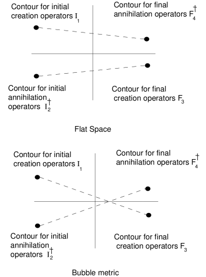
Figure 1: The complex $t$ plane for the calculations of the superscattering operator, showing how the Wightman functions are integrated over contours with a small imaginary time displacement. The upper diagram corresponds to flat space and the lower to the extra scalar products that occur in the identified sphere bubble.

On the identified four sphere however, the data from the final state annihilation operators $F_{4}^{\dagger}$ will also propagate downwards from an image of the contour $4$ below the real $u$ axis. It thus can have a nonzero scalar product with the contour $2$ on which the initial state annihilation operators $I_{2}^{\dagger}$ act. Similarly, there can be a non zero scalar product between the data from the final state creation operators $F_{3}$ and the initial state creation operators $I_{1}$ (Figure 1).

These scalar products have been calculated for conformally invariant fields of spin $s$ propagating on this background. For each particle with initial and final momenta $k_{2}^{\mu}$ and $k_{4}^{\mu}$, the $4\rightarrow 2$ scalar product gives a factor

$$\langle k_{4}|k_{2}\rangle=-{q^{2}\over 8\pi}e^{ip\cdot(k_{2}+k_{4})}J_{2s}\left(\left[-{1\over 2}k_{2}\cdot k_{4}q^{2}+(q\cdot k_{2})(q\cdot k_{4})\right]^{1/2}\right),$$

where $p^{\mu}={1\over 2}(x_{q}^{\mu}+x_{r}^{\mu})$ and $q^{\mu}=x_{q}^{\mu}-x_{r}^{\mu}$. The scalar product $3\rightarrow 1$ has a similar factor for each particle, but $k_{1}^{\mu}$ and $k_{3}^{\mu}$ appear with the opposite signs.

There will be factors like this for each of the $n$ particle lines passing through the bubble. There will also be a factor $\Delta^{-1/2}\exp(-I)$ where $\Delta$ is the determinant of the conformally invariant field wave operator and $I={3\over 8}\pi q^{2}$ is the action of the asymptotically Euclidean bubble metric. One them integrates over the positions of the points $q$ and $r$ or equivalently over the vectors $p$ and $q$. The integral over all $p$ produces $\delta(k_{2}+k_{4}-k_{3}-k_{1})$. This does not guarantee energy momentum conservation because it would be satisfied by $k_{1}=k_{2}\neq k_{3}=k_{4}$. As discussed below, energy momentum conservation comes from the path integral over all metrics equivalent under diffeomorphisms. The integral over all $q$ averages over the orientation and scale of the bubble metric. The dominant contribution to the integral over the scale will come from bubbles of order the Planck size.

These nonzero scalar products that would not occur in flat space have two consequences. First, consider a field $\phi$ with a global symmetry such as $U(1)$ that is not coupled to a gauge field. Take the initial state operators $I_{1}$ and $I_{2}$ to be particle creation operators and the final state operators $F_{3}$ and $F_{4}$ to be anti-particle creation operators. Then there will be a nonzero probability for a particle to change into its anti-particle. This is what one would expect. In the presence of black holes, real or virtual, global charges will not be conserved. However, if the particles are coupled to a gauge field, averaging over gauges will make the amplitude zero unless the gauge charge is conserved. Similarly, averaging over diffeomorphisms, the gravitational gauge degrees of freedom, should ensure that the amplitude is zero unless energy is conserved. As was seen above, energy conservation is not guaranteed by integration over the position of the bubble. When there is loss of quantum coherence, it is only local symmetries and not global ones that imply conservation laws.

The second consequence of the nonzero scalar products is that the $\$$ operator giving the probability to go from initial to final will not factorise into an $S$ matrix times its adjoint. This means that the evolution from initial to final will be non-unitary and will exhibit loss of quantum coherence. This is what you might expect in a bubble with non-trivial topology, because the Euler number of three will mean that one cannot foliate the spacetime with a family of time surfaces. One thus cannot show there is a unitary Hamiltonian evolution. However, any suggestion that quantum coherence may be lost seems to arouse furious opposition. It is almost like I was attacking the existence of the ether.

4 Scattering by black hole loops

The metric considered in the last section was a special limiting case of an asymptotically Euclidean $S^{2}\times S^{2}-\{p\}$ metric. However, one might be concerned that because it so special, scattering in it would not be typical of $S^{2}\times S^{2}-\{p\}$ bubbles. In this section I shall therefore consider scattering in a different class of metrics that correspond more directly with the intuitive picture of $S^{2}\times S^{2}$ bubbles as closed loops of real or virtual black holes.

One cannot analytically continue a general real Euclidean metric to a section of the complexified manifold on which the manifold is real and Lorentzian. This does not matter for scattering calculations, because one can analytically continue to Lorentzian at infinity, and one does not directly measure the metric at interior points, but one integrates over all possible metrics. The idea is that the path integral over all Lorentzian metrics is equivalent to a path integral over all Euclidean ones in a contour integral sense. However, in order to give the scattering a physical interpretation, it is helpful to consider metrics that have both Euclidean and Lorentzian sections. This will be guaranteed if the metric has a hypersurface orthogonal Killing vector. If the metric is asymptotically Euclidean, one can interpret this Killing vector as corresponding to a Lorentz boost at infinity. For simplicity, I shall also assume that there is a second commuting hypersurface orthogonal Killing vector corresponding to rotations about an axis. The is the maximum symmetry that an asymptotically Euclidean metric on $S^{2}\times S^{2}-\{p\}$ can have. In particular, virtual black holes can not be spherically symmetric.

The Lorentzian section of the metric will have a structure like that of the $C$ metric or the Ernst solution, with two black holes accelerating away from each other. By the positive action theorem, there are no asymptotically Euclidean solutions of the vacuum Einstein equations with topology $S^{2}\times S^{2}-\{p\}$. The $C$ metric has singularities on the axis, which can be interpreted as cosmic strings pulling the black holes apart, and the Ernst solution is asymptotic not to flat Euclidean space, but to the Euclidean Melvin solution. However, as was said earlier, I shall consider asymptotically Euclidean metrics on $S^{2}\times S^{2}-\{p\}$ that correspond not to real black holes, but to virtual black hole loops that arise as vacuum fluctuations. These will not be solutions of the Einstein equations, and will be similar to the $C$ metrics, but without singularities on the axis.

The Lorentzian metrics will be asymptotically flat with zero mass. They will have good past and future null infinities $\cal I^{-}$ and $\cal I^{+}$, which are the light cones of the point $p$ at infinity in the conformally compactified Euclidean metric or the spatial infinity point $I^{0}$ in the conformally compactified Lorentzian metric. The boost Killing vector $\xi$ and the axisymmetric Killing vector $\eta$ can be extended to $\cal I^{\pm}$. On $\cal I^{+}$, $\xi$ will have two fixed points, $q_{l}^{+}$ and $q_{r}^{+}$, on the left and right of figure 2. The past light cones of these fixed points, apart from the two generators $\gamma_{l}^{+}$ and $\gamma_{r}^{+}$, which lie in $\cal I^{+}$, form the left and right acceleration horizons ${\cal H}_{al}$ and ${\cal H}_{ar}$. These light cones focus again to two fixed points $q_{r}^{-}$ and $q_{l}^{-}$ on the right and left of $\cal I^{-}$ respectively. The acceleration horizons divide the region outside the black holes into the left and right Rindler wedge, labelled IV and II, and the future and past regions, labelled I and III.

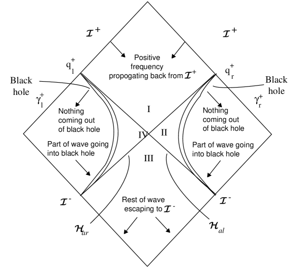
Figure 2: The Lorentzian section of an asymptotically Euclidean metric on $S^{2}\times S^{2}-{pt}$.

There are also two black hole horizons ${\cal H}_{bl}$ and ${\cal H}_{br}$. The horizon ${\cal H}_{bl}$ consists of ${\cal H}_{bl}^{+}$, the future horizon of the left black hole, and ${\cal H}_{bl}^{-}$, the past horizon of the right black hole. Similarly, ${\cal H}_{br}$ consists of the future horizon of the right black hole and the past horizon of the left black hole.

The region outside the black holes is globally hyperbolic. One can therefore analyse the behaviour of a massless field $\phi$ in a manner similar to that on static black holes [10]. One can take a past Cauchy surface to be $\cal I^{-}$ and the past left and right black hole horizons ${\cal H}_{br}^{-}$ and ${\cal H}_{bl}^{-}$. Similarly, $\cal I^{+}$ and future black hole horizons will form a future Cauchy surface. Now consider a solution $\mu$ of the wave equation which has positive frequency on $\cal I^{+}$ with respect to the affine parameter and zero data on on the future black hole horizons. As Yi [11] has pointed out, it is reasonable to ignore $\gamma_{l}^{+}$ and $\gamma_{r}^{+}$ as sets of measure zero on $\cal I^{+}$, and to take the support of $\mu$ to be away from them. In other words, one ignores waves directed exactly along the axis asymptotically.

In this case, $\mu$ will propagate backwards through the future region I to the future V formed by the future halves of the acceleration horizons. On ${\cal H}_{al}^{+}$ and ${\cal H}_{ar}^{+}$ one can decompose $\mu$ into modes with definite frequency $\omega^{\prime}$ with respect to the Rindler time associated with the boost Killing vector $\xi$. One can also separate into eigenmodes with respect to the axial Killing vector $\eta$, but the wave equation probably cannot be separated in the remaining two dimensions. I shall therefore label the eigenmodes $\psi_{\omega^{\prime}mn}$ where $n$ labels the eigenmodes of the wave equation in the remaining two dimensions.

One can now consider the wave equation in the right hand Rindler wedge II. Since one is ignoring $\gamma_{r}^{+}$ as a set of measure zero, a Cauchy surface for this region will be the future acceleration horizon ${\cal H}_{ar}^{+}$ and the future black hole horizon ${\cal H}_{br}^{+}$. The data for $\mu$ will be zero on ${\cal H}_{br}^{+}$ (by assumption), and will be a mixture of eigenmodes $\psi_{\omega^{\prime}mn}$ on ${\cal H}_{ar}^{+}$. A fraction $\Gamma_{\omega^{\prime}mn}$ of the flux of each eigenmode will cross the past black hole horizon ${\cal H}_{bl}^{-}$, and the remaining $(1-\Gamma_{\omega^{\prime}mn})$ will reflect on the effective potential and will cross the past acceleration horizon ${\cal H}_{al}^{-}$. Similarly, one can solve the wave equation in the left hand Rindler wedge IV and find that a fraction $\Gamma_{\omega^{\prime}mn}$ goes into the black hole and a fraction $(1-\Gamma_{\omega^{\prime}mn})$ crosses the past acceleration horizon.

One now has data on the two past acceleration horizons ${\cal H}_{al}^{-}$ and ${\cal H}_{ar}^{-}$ and can solve the wave equation on the past region III. For each eigenmode, the data on the left and right acceleration horizons will both be reduced by the same factor $(1-\Gamma_{\omega^{\prime}mn})^{1/2}$. Thus it seems likely that $\mu$ will be purely positive frequency on $\cal I^{-}$. However, it will not be purely positive frequency on the black hole horizons, because it is non zero on the past parts ${\cal H}_{br}^{-}$ and ${\cal H}_{bl}^{-}$ but it is zero by assumption on the future parts ${\cal H}_{bl}^{+}$ and ${\cal H}_{br}^{+}$. This means that an observer at $\cal I^{+}$ will observe particles in the mode $\mu$, contrary to the claims of Yi [11]. Another way of saying this is that the positive frequencies from the final state creation operators $F_{3}$ on $\cal I^{+}$ will have a non zero scalar product with the final state annihilation operators $F_{4}^{\dagger}$, so that

$$\langle F_{3}F_{4}^{\dagger}\rangle\neq 0.$$

Similarly, the positive frequencies from the initial creation operators $I_{1}$ can go into the black holes and have a non zero scalar product with the initial annihilation operators. This gives a diagram like Figure 3. Note that the initial annihilation and creation operators can belong to different particle species from those of the final operators. This is what one might expect because the No Hair theorems imply that a black hole forgets what fell into it apart from charges coupled to gauge fields. It means that the full superscattering matrix element will not factorise. Further discussion of scattering in metrics of this type will be given in another paper.

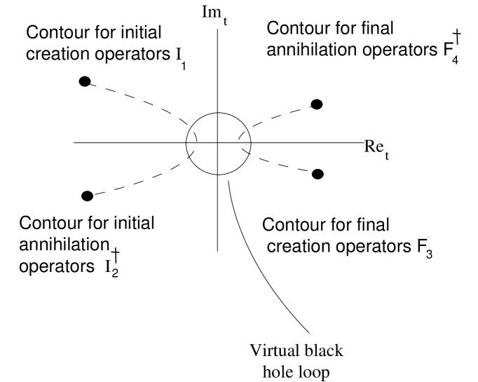
Figure 3: The complex $t$ plane for scattering on an asymptotically Euclidean virtual black hole metric.

5 Observational consequences

Obviously, quantum coherence is not lost under normal conditions to a very high degree of approximation, so one has to ask what order of magnitude the bubble scattering calculation would indicate. It seems that the scattering at low energies depends strongly on the spin of the field. One can see this explicitly in the case of the identified sphere metric in section 3. Here the amplitudes were products of Bessel functions $J_{2s}(c)$ for each pair of momenta, where $s$ was the spin and $c$ was a quantity of order of the center of mass energy in the scattering. For low energy scatterings, $c\ll 1$,

$$J_{2s}(c)\approx c^{2s}.$$

These amplitudes are of the same order as those that would be produced by effective interactions of the form

$$m_{p}^{4-2n(1+s)}(\phi)^{2n},$$

where $n\geq 2$ is the number of pairs of ingoing or outgoing momenta scattered through the bubble. The field $\phi$ in the effective interaction is the scalar field for $s=0$ and the spinor field for $s={1\over 2}$. For $s=1$, it is the field strength $F_{\mu\nu}$. The scattering calculations have not been done explicitly for spin $3\over 2$ and $2$, but on this basis one would expect the effective interactions to involve the gradient of the spin $3\over 2$ field and the curvature respectively.

One would like to know whether this spin dependence of the scattering is peculiar to the special bubble metric considered in section 3, or whether it is a general feature. In fact, consideration of scattering in the more general metrics of section 4 suggests that the effective interactions depend on spin in a similar way. The non-factoring part of the scattering can be thought of as a scattering cross section for a wave to get into a black hole and a thermal factor. Calculations of scattering by static black holes indicate that for black holes much smaller than the wave length $\omega^{-1}$, the absorption cross sections are of the order of the geometrical cross sections for both $s=0$ and $s={1\over 2}$, while they are of order $\omega^{2}$ for $s=1$. The Bose-Einstein thermal factor will be of order $\omega^{-1}$ while the Fermi-Dirac factor will be order $1$. Thus one will get the same $c^{2s}$ dependence on spin. It is therefore reasonable to suppose that any bubble metric will give effective interactions of the same order.

The effective interactions induced by bubbles are local, in that the scale of the bubble will be of order the Planck length, while the center of mass wavelength will be larger for low energy scatterings. However, they will be nonlocal in that they will mix up the separation that one has in flat space between the diagrams for the $S$ matrix and its adjoint. This separation is of order $\epsilon$, and one takes the limit $\epsilon\rightarrow 0$. Thus the separation will become less than the size of the bubble. If the effective interactions had been purely local, they would have produced a unitary evolution, but the fact that they are nonlocal means that quantum coherence can be lost [12, 13].

One can see that almost all these effective interactions are suppressed by factors of the Planck mass. The only exceptions are scalar fields, which would get an effective $\phi^{4}$ or $\phi^{2}\phi^{2}$ interaction, with coefficients of order one. But we have never yet observed an elementary scalar field. Particles like the pion are really bound states of fermions. When scattering off a bubble, they would behave like individual fermions. This suggests that we may never observe the Higgs particle, because it will be strongly coupled to every other scalar field, or that if we do detect it, it will turn out to be a bound state of fermions.

Effective interactions between fermions will be suppressed by two powers of the Planck mass for a four fermion vertex and five powers for a six fermion vertex. The first could contribute to $K_{L}^{0}$ decay and the second to baryon decay. However, the lifetimes are of the order of $10^{7}$ and $10^{64}$ years respectively, so they are not of much experimental interest. The quantum coherence violating effective interactions induced between spin $1$ fields are even more suppressed, so we wouldn’t have observed them. On the other hand, there might be a $\psi^{2}\phi^{2}$ fermion scalar effective interaction that was suppressed by only one power of the Planck mass. The possible consequences of such an interaction will be investigated elsewhere.

Another observational feature that might be explained by loss of quantum coherence is the fact that the $\theta$ angle of QCD is zero. One way of interpreting the $\theta$ angle is to regard the QCD vacuum as a coherent sum

$$\sum e^{i\theta}|n\rangle$$

of states labelled with a winding number $n$. Although there are no asymptotically Euclidean vacuum solutions, there are asymptotically Euclidean Einstein-Maxwell solutions. These have an asymptotically self dual uniform Maxwell field at infinity. They were investigated by one of my students, Alan Yuille, and are in his PhD thesis, but are otherwise unpublished. If one takes a $U(1)$ subgroup of a Yang-Mills group, one can promote them to Einstein-Yang-Mills solutions. The ordinary Yang-Mills instantons in flat space have self dual Yang-Mills fields which can be taken to be uniform over sufficiently small regions. Thus one could imagine glueing small bubbles on to a flat space Yang-Mills instanton and obtaining an instanton with warts that was a solution of the field equations. One might expect that the bubbles, or warts, would produce loss of coherence between the different $|n\rangle$ vacua. In other words, there would be a nonzero probability to go from the product density matrix

$$\sum e^{i(n-m)\theta}|n\rangle\langle m|$$

to a density matrix with other coefficients. Presumably the density matrix would tend to the state with lowest energy, which is probably the $\theta=0$ density matrix with equal coefficients.

If $\theta$ were nonzero (and in flat space Yang-Mills theory, there is no reason why it shouldn’t be), it would have produced effects like a dipole moment for the neutron, which would have been observed. To explain the absence of a dipole moment, the Peccei-Quinn [14] mechanism was proposed. The original version of the mechanism was ruled out because it predicted an axion of a few hundred KeV mass that was not observed. There was a grand unified theory version of the mechanism, which would have given rise to a very light and weakly interacting axion. At one time, it was hoped that this axion might make up the cold dark matter required to give the universe the critical density. However, recent work on the damping of axion cosmic strings [15] has almost closed the window of possible masses for the axion. So we badly need an explanation of the zero dipole moment of the neutron. My bet is that it is loss of quantum coherence.

In the case of the wormhole picture, it seemed at first that quantum coherence would be lost because wormholes would connect the upper and lower halves of diagrams for the $\$$ matrix. However, it turned out that that effects of wormholes on low energy physics could be described by a number of alpha parameters [2]. These would act as the coupling constants for ordinary local effective interactions that didn’t lose quantum coherence. Their values wouldn’t be determined by the theory. However, one could conduct experiments to measure all the effective coupling constants up to a certain order. After that, there would be no unpredictability or loss of quantum coherence. One would have ordinary quantum field theory with coupling constants that couldn’t be predicted but could be chosen to agree with experiment.

Could the situation be similar with the quantum bubbles picture? Could the unpredictability associated with loss of quantum coherence be absorbed into a lack of knowledge of coupling constants? I can’t rule this out, but I don’t think it will be the case. There is an important difference between the wormhole and bubble pictures. With wormholes, one can integrate over the position of each end of the wormhole separately. This allows the effect of the wormhole to be factorised into separate local interactions at each end of the wormhole. However, with a quantum bubble, there is only one integral over the position of the bubble. Thus, one cannot factorise the effect of a bubble. It will therefore give rise to a nonlocal interaction that connects the evolution of a quantum state with that of its complex conjugate. I therefore expect that when one sums over all the bubbles in spacetime foam, one will still get loss of quantum coherence.

6 Evaporation of macroscopic black holes

The picture of virtual black holes as occurring in pairs and corresponding to $S^{2}\times S^{2}$ topological fluctuations has implications for the end point of the evaporation of a macroscopic black hole. For twenty years, I tried to think of a Euclidean geometry that would describe the disappearance of a single black hole. But the only thing that seemed possible was a wormhole, and I have already said why I came to reject that idea. However, I now think that when a black hole evaporates down to the Planck size, it won’t have any energy or charge left, and it will just disappear into the sea of virtual black holes. If this picture is correct, it implies that two dimensional models can’t describe the disappearance of black holes in a way that is nonsingular. This agrees with our experience. The best we can do in two dimensions is the RST [16] model. In this, a black hole evaporates down to zero mass. However, one then has to cut the solution off by hand and join on the vacuum solution. This is very ad hoc and introduces a naked singularity. Strominger and Polchinski [17] have tried to argue that a baby universe branches off. However, I think that is wrong for the reasons for which I rejected the wormhole scenario.

7 Conclusions

It seems that topological fluctuations on the Planck scale should give spacetime a foam-like structure. The wormhole scenario and the quantum bubbles picture are two forms this foam might take. They are characterized by very large values of the first and second Betti numbers respectively. I argued that the wormhole picture didn’t really fit with what we know of black holes. On the other hand, pair creation of black holes in a magnetic field or in cosmology is described by instantons with topology $S^{2}\times S^{2}$. This shows that one can interpret $S^{2}\times S^{2}$ topological fluctuations as closed loops of virtual black holes.

I then went on to discuss particle scattering by $S^{2}\times S^{2}$ bubbles. Because of the non-trivial topology, one cannot cover the manifold with a family of time surfaces. One cannot therefore act with a Hamiltonian and get a unitary evolution from the initial state to the final one. It is therefore possible that quantum coherence could be lost, and I showed that indeed it was, both explicitly, in a simple bubble metric, and in more general cases. I gave estimates of the magnitude of bubble induced effects. They are all suppressed by powers of the Planck mass, with the exception of scalar fields. We have not yet observed an elementary scalar particle, and I predict we never will. Another prediction of the quantum bubbles picture is that the $\theta$ angle of QCD should be exactly zero, without having to invoke the existence of an axion. This is almost ruled out by observation, anyway. There may well be other predictions of the quantum bubble picture which are testable at low energy. Thus, the question of the Planck scale structure of spacetime may not be as esoteric as it is sometimes made out to be. In the fluctuations in the microwave background, we are already observing effects on scales of about $10^{6}$ Planck lengths. This would have been the horizon size of the universe at the time the fluctuations were produced during inflation. So quantum gravity is real physics. I think it is quite possible that we can observe the consequences of spacetime structure on even smaller scales. This will be one of the challenges for the next few years. Unless quantum gravity can make contact with observation, it will become as academic as arguments about how many angels can dance on the head of a pin.

References

- [1] S. W. Hawking, Phys. Rev. D 37, 904 (1988).
- [2] S. Coleman, Nucl. Phys. B130, 643 (1988).
- [3] S. W. Hawking, Nucl. Phys. B144, 349 (1978).
- [4] F. J. Ernst, J. Math. Phys. 17, 515 (1976).
- [5] H.F. Dowker, J.P. Gauntlett, D.A. Kastor and J. Traschen, Phys. Rev. D 49, 2909 (1994).
- [6] S.F. Ross, Phys. Rev. D 49, 6599 (1994).
- [7] G.W. Gibbons, in Fields and Geometry 1986, Proceedings of the 22nd Karpacz Winter School of Theoretical Physics, Karpacz, Poland, edited by A. Jadczyk (World Scientific, Singapore, 1986).
- [8] S.W. Hawking, D.N. Page and C.N. Pope, Nucl. Phys. B170, 283 (1980).
- [9] S.W. Hawking, Commun. Math. Phys. 87, 395 (1982).
- [10] S. W. Hawking, Commun. Math. Phys. 43, 199 (1975).
- [11] P. Yi, Phys. Rev. Lett. 75, 382 (1995); P. Yi, “Quantum stability of accelerated black holes”, preprint CU-TP-690, hep-th/9505021.
- [12] T. Banks, L. Susskind and M.E. Peskin, Nucl. Phys. B244, 125 (1984).
- [13] W.G. Unruh and R.M. Wald, Phys. Rev. D 52, 2176 (1995).
- [14] R.D. Peccei and H.R. Quinn, Phys. Rev. Lett. 38, 1440 (1977).
- [15] R.A. Battye and E.P.S. Shellard, Phys. Rev. Lett. 73, 2954 (1994).
- [16] J.G. Russo, L. Susskind and L. Thorlacius, Phys. Rev. D 46, 3444 (1992).
- [17] J. Polchinski and A. Strominger, Phys. Rev. D 50, 7403 (1994).