CERN-TH/95-254

After recalling a few basic concepts from cosmology and string theory, I will outline the main ideas/assumptions underlying (our own group’s approach to) string cosmology and show how these lead to the definition of a two-parameter family of “minimal” models. I will then briefly explain how to compute, in terms of those parameters, the spectrum of scalar, tensor and electromagnetic perturbations, and mention their most relevant physical consequences. More details on the latter part of this talk can be found in Maurizio Gasperini’s contribution to these proceedings.

Talk presented at the

3rd Colloque Cosmologie, Paris

7-9 June 1995

CERN-TH/95-254

September 1995

1 Basic Facts about Cosmology and Inflation

It is well known¹⁾ that the Standard Cosmological Model (SCM) works well at “late” times, its most striking successes being perhaps the red shift, the cosmic microwave background (CMB), and primordial nucleosynthesis.

However, the SCM suffers from various problems. At the theoretical level the most serious of these is the initial singularity problem, which basically tells us that we cannot have theoretical control over the initial conditions of the SCM. At a phenomenological level, the SCM cannot explain naturally:

• the homogeneity and isotropy of our Universe as manifested, in particular, through the small value of $\Delta T/T=O(10^{-5})$ observed with COBE²⁾;

• the flatness problem, i.e. the fact that, within an order of magnitude, $\Omega\equiv\rho/\rho_{crit}\sim 1$;

• the origin of large-scale structure.

Inflation, i.e. a long phase of accelerated expansion of the Universe ($\dot{a},\ddot{a}>0$, where $a$ is the scale factor), is the only way known at present of solving the above-mentioned phenomenological problems. Various types of inflationary models have been proposed [for a review, see 3), 4)] each one supposedly mending the problems of the previous version. Particularly severe are the constraints coming from demanding:

a) a graceful exit with the right amount of reheating;

b) the right amount of large-scale inhomogeneities.

In order to satisfy such constraints, fine-tuned initial conditions and/or inflaton potentials are necessary. And this without mentioning the fact that inflation is not addressing at all the initial singularity problem.

Actually, Kolb and Turner, after reviewing the prescriptions for a successful inflation, add⁴⁾:

“Perhaps the most important – and most difficult – task in building a successful inflationary model is to ensure that the inflaton is an integral part of a sensible model of particle physics. The inflaton should spring forth from some grander theory and not vice versa”.

I will argue below that superstring theory could be the sought-after grander theory (what could be better than a theory of everything?) naturally providing an inflation-driving scalar field in the general sense defined again in ref. 4):

“It is now apparent that inflation, which was originally so closely related to Spontaneous Symmetry Breaking, is a much more general phenomenon…. Stated in its full generality, inflation involves the dynamical evolution of a very weakly-coupled scalar field that was originally displaced from the minimum of its potential.”

I hope to convince you that this will be precisely the picture that we claim takes place in string cosmology. In order to substantiate this claim, I will have to digress and recall a few basic facts in Quantum String Theory.

2 Basic facts in quantum string theory (QST)

I am listing below a few basic properties of strings, emphasizing those that are most relevant for our subsequent discussion. These are:

1. Unlike its classical counterpart, quantum string theory contains a fundamental length scale $\lambda_{s}$. Such a scale appears in many physical quantities. It represents, for instance:

• Planck’s constant (in appropriate units of energy) ⁵⁾.

• The ultraviolet, short-distance cut-off (equivalently, a high-momentum cut-off at $E=M_{s}\equiv\hbar c/\lambda_{s}$).

• The scale of tree-level masses that are either zero or $O(M_{s})$. Incidentally, quantum mechanics allows massless strings with non-zero angular momentum⁶⁾ while, classically, $M^{2}>{\rm const.}\times J$. The existence of such states is obviously a crucial property of QST, without which it could not pretend to be a candidate theory of all known interactions.

2. The absence of free parameters $(c=\lambda_{s}=1$ simply defines the units of length and time and are in priciple known numbers once the centimetre and the second are defined), which are replaced by expectation values of fields⁶⁾. Basically, some huge (and still largely unknown) symmetry should fix the tree-level “Lagrangian”, while UV finiteness [point 1b)] preserves full predictive power at loop level. Note again here the contrast with quantum field theory (QFT), where, even if the bare couplings were fixed, the need to renormalize the theory at loop level would make the renormalized constants finite but uncalculable.

3. The effective interaction of the massless fields at $E\ll M_{s}$ is dictated by the above symmetries and takes the form of a classical, gauge-plus-gravity field theory with specified parameters. It is described by an effective action^7),8) of the (schematic) type:

$$\Gamma_{eff} = \frac{1}{2}\int d^{4}x\sqrt{-g}~{}e^{-\phi}\left[\lambda^{-2}_{s}({\cal R}+\partial_{\mu}\phi\partial^{\mu}\phi)+F^{2}_{\mu\nu}+\bar{\psi}D\hbox to0.0pt{\hss$/$}\psi+{\rm higher~{}derivatives}\right]$$ (2.1)

$$+\left[{\rm higher~{}orders~{}in}~{}e^{\phi}\right]~{}.$$

Equation (2.1) contains two dimensionless expansion parameters. One of them, $g^{2}\equiv e^{\phi}$, controls the analogue of QFT’s loop corrections, while the other, $\lambda^{2}\equiv\lambda_{s}^{2}\cdot\partial^{2}$, controls string-size effects, which are of course absent in QFT.

4. As indicated in (2.1), QST has (actually needs!) a new particle/field, the so-called dilaton $\phi$, a scalar massless particle (at the perturbative level). It appears in $\Gamma_{eff}$ as a Jordan–Brans–Dicke⁹⁾ scalar with a “small” negative $\omega_{BD}$ parameter, $\omega_{BD}=-1$.

5. The dilaton’s VEV provides^8),10) a unified value for:

• The gauge coupling(s) at $E=O(M_{s})$.

• The gravitational coupling in string units.

• Yukawa couplings, etc., at the string scale.

In formulae:

$$\ell^{2}_{p} \equiv 8\pi G_{N}\hbar=e^{\phi}\lambda^{2}_{s}~{},$$

$$\alpha_{GUT}(\lambda^{-1}_{s}) \simeq \frac{e^{\phi}}{4\pi}~{},$$ (2.2)

implying (from $\alpha_{GUT}\approx 1/20$) that the string-length parameter $\lambda_{s}$ will be about 10^-32 cm. Note, however, that, in a cosmological context in which $\phi$ evolves in time, the above formulae can only be taken to give the $\it{present}$ values of $\alpha$ and $\ell_{p}/\lambda_{s}$. In the scenario we will advocate, both quantities were much smaller in the very early Universe!

6. Dilaton couplings at large distance are essentially known¹¹⁾ and can be summarized in the following effective Lagrangian (taking loop effects into account):

$${\cal L}_{eff} = \sum_{i}g_{\phi A_{i}A_{i}}\phi A^{2}_{i}$$

$$g_{\phi A_{i}A_{i}} = \sqrt{4\pi G}m^{2}_{i}Z_{\phi}^{-1/2}\left.(\frac{\partial}{\partial\phi}ln\frac{m^{2}_{i}}{M_{P}^{2}})\right|_{\phi=\langle\phi\rangle}~{}.$$ (2.3)

Here $\sqrt{4\pi G}m^{2}_{i}$ is the same strength as for (static) gravity, the correction $Z^{1/2}_{\phi}$ is $1+O(\alpha_{GUT})$, while the last factor is computable if $e^{\phi}$ is reasonably small. One finds¹¹⁾ that the dilaton coupling to nuclear matter (QCD confinement mass) is about 80 times larger than gravity. Furthermore, since the coupling to electromagnetic mass or to leptons is expected to be substantially different (probably smaller), one predicts a composition-dependent “5th force” of strength larger than gravity. Tests of the equivalence principle down to ranges of $10^{-1}$ - 1  cm¹²⁾ thus put bounds^11),13) on the dilaton mass [for a possible way out see, however, ref. 14)], i.e.

$$M_{\phi}>10^{-4}~{}{\rm eV}~{}.$$ (2.4)

7. Details about the dilaton potential are unknown, yet:

• On theoretical grounds, in critical superstring theory, the dilaton potential has to go to zero as a double exponential as $\phi\rightarrow-\infty$ (weak coupling):

  $$V(\phi)\sim{\rm exp}\left(-c^{2}{\rm exp}(-\phi)\right)={\rm exp}\left(-\frac{c^{2}}{4\pi\alpha_{GUT}}\right)~{},$$ (2.5)

  with $c^{2}$ a positive (but model-dependent) constant.

• On physical grounds it should have a non-trivial minimum at its present value ($\langle\phi\rangle=\phi_{0}\sim 0)$ with a vanishing cosmological constant, $V(\phi_{0})=0$.

A typical potential satisfying a) and b) is shown in Fig. 1. The dotted lines at $\phi>0$ represent our ignorance about strongly coupled string theory. Fortunately, the details of what happens in that region will not be very relevant for our subsequent discussion.

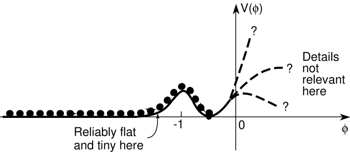
Figure 1: A possible dilaton potential with illustration of an inflation-driving rolling dilaton (large dots).

8. There is an exact (all-order) vacuum solution for (critical) superstring theory. Unfortunately, it corresponds to a free theory ($g=0$ or $\phi=-\infty$) in flat, ten-dimensional, Minkowski space-time, nothing like the world we seem to be living in!

3 The main ideas/assumptions of string cosmology

The very basic postulate of (our own version of) String Cosmology^15),16) is that the Universe did indeed start near its trivial vacuum mentioned at the end of the previous section.

Fortunately, if one looks at the space of homogeneous (and for simplicity spacially-flat) perturbative vacuum solutions, one finds that the trivial vacuum is a very special, $\it{unstable}$ solution. This is depicted in Fig. 2a for the simplest case of a ten-dimensional cosmology in which three spatial dimensions evolve isotropically while six “internal” dimensions are static (it is easy to generalize the discussion to the case of dynamical internal dimensions, but then the picture becomes multidimensional).

The straight lines in the $H,\dot{\bar{\phi}}$ plane (where $\dot{\bar{\phi}}\equiv\dot{\phi}-3H$) represent the evolution of the scale factor and of the coupling constant as a function of the cosmic time parameter (arrows along the lines show the direction of the time evolution). As a consequence of a stringy symmetry, known^15),17) as “Scale Factor Duality (SFD)”, there are two branches (two straight lines). Furthermore, each branch is split by the origin in two time-reversal-related parts (time reversal changes the sign of both $H$ and $\dot{\bar{\phi}}$).

The origin (the trivial vacuum) is an “unstable” fixed point: a small perturbation in the direction of positive $\dot{\bar{\phi}}$ makes the system evolve further and further from the origin, meaning larger and larger coupling and absolute value of the Hubble parameter. This means an accelerated expansion or an accelerated contraction, i.e. in the latter case, inflation. It is tempting to assume that those patches of the original Universe that had the right kind of fluctuation have grown up to become (by far) the largest fraction of the Universe today.

In order to arrive at a physically interesting scenario, however, we have to connect somehow the top-right inflationary branch to the bottom-right branch, since the latter is nothing but the standard FRW cosmology, which has presumably prevailed for the last few billion years or so. Here the so-called “exit problem” arises. At lowest order in $\lambda^{2}$ (small curvatures in string units) the two branches do not talk to each other. The inflationary (also called $+$) branch has a singularity in the future (it takes a finite cosmic time to reach $\infty$ in our gragh if one starts from anywhere but the origin) while the FRW ($-$) branch has a singularity in the past (the usual big-bang singularity).

It is widely believed that QST has a way to avoid the usual singularities of Classical General Relativity or at least a way to reinterpret them^18),19). It thus looks reasonable to assume that the inflationary branch, instead of leading to a non-sensical singularity, will evolve into the FRW branch at values of $\lambda^{2}$ of order unity. This is schematically

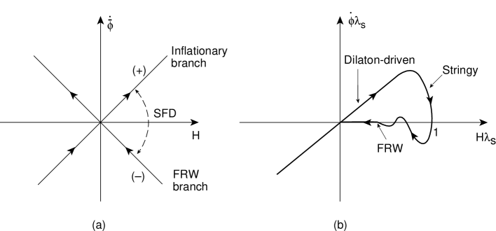
Figure 2: Phase diagrams for the perturbative (a) regime and a conjectured non-perturbative solution (b) to the branch-change problem.

shown in Fig. 2b, where we have gone back from $\dot{\bar{\phi}}$ to $\dot{\phi}$ and we have implicitly taken into account the effects of a non-vanishing dilaton potential at small $\phi$ in order to freeze the dilaton at its present value. The need for the branch change to occur at large $\lambda^{2}$, first argued for in²⁰⁾, has been recently proved in ref. 21).

There is a rather simple way to parametrize a class of scenarios of the kind defined above. They contain (roughly) three phases and two parameters. Indeed:

In phase I the Universe evolves at $g^{2},\lambda^{2}\ll 1$ and thus is close to the trivial vacuum. This phase can be studied using the tree-level low-energy effective action (2.1) and is characterized by a long period of dilaton-driven inflation. The accelerated expansion of the Universe, instead of originating from the potential energy of an inflaton field, is driven by the growth of the coupling constant (i.e. by the dilaton’s kinetic energy, see ref. 22) for a similar kind of inflationary scenario) with $\dot{\phi}=2\dot{g}/g\sim H$ during the whole phase.

Phase I supposedly ends when the coupling $\lambda^{2}$ reaches values of $O(1)$, so that higher-derivative terms in the effective action become relevant. Assuming that this happens while $g^{2}$ is still small (and thus the potential is still negligible), the value $g_{s}$ of $g$ at the end of phase I (the beginning of phase II) is an arbitrary parameter (a modulus of the solution).

During phase II, the stringy version of the big bang, the curvature, as well as $\dot{\phi}$, are assumed to remain fixed at their maximal value given by the string scale (i.e. we expect $\lambda\sim 1$). The coupling $g$ will instead continue to grow from the value $g_{s}$ until it is its own turn to reach values $O(1)$. At that point, assuming a branch change to have occurred at large curvatures, the dilaton will be attracted to the true non-perturbative minimum of its potential; the standard FRW cosmology can then start, provided the Universe was heated-up and filled with radiation (this is not a problem, see below). The second important parameter of this scenario is the duration of phase II or better the total red-shift, $z_{s}\equiv a_{end}/a_{beg}$, which has occurred from the beginning to the end of the stringy phase.

Our present ignorance about this most crucial phase (and in particular about the way the exit can be implemented) prevents us from having a better description of this phase which, in principle, should not introduce new arbitrary parameters ($z_{s}$ should be eventually determined in terms of $g_{s}$).

During Phase III, the Universe evolves towards smaller and smaller curvatures but stays at moderate-to-strong coupling. This is the regime in which usual QFT methods are applicable. The details of the particular gauge theory emerging from the string’s non-perturbative vacuum will be very important in determining the subsequent evolution and in particular the problem of structure formation, dark matter and the like.

Our scenario contains implicitly an arrow of time, which points in the direction of increasing entropy, inhomogeneity and structure. As a result of the amplification of primordial vacuum fluctuations, the Universe is not coming back to its initial simple (and unique) state (the origin in Fig. 2), but to the much more structured (and interesting) state in which we are living today. Actually, the arrow of time itself should be determined by the direction in which entropy (and complexity) are growing. This will force us to identify ($\it{by~{}definition}$) the perturbative vacuum with the initial state of the Universe!

4 Observable consequences

All the observable consequences I will discuss below have something to do with the well-known phenomenon²³⁾ of amplification of vacuum quantum fluctuations in cosmological backgrounds. Any conformally flat cosmological background is known:

• to amplify tensor perturbations, i.e. to produce a stochastic background of gravitational waves;

• to induce scalar-metric perturbations from the coupling of the metric either to a fluid or to scalar particles (in our context to the dilaton).

By contrast, because of the scale-invariant coupling of gauge fields in four dimensions, electromagnetic (EM) perturbations are $\it{not}$ amplified in a conformally flat cosmological background (even if inflationary). In string cosmology, the presence of a time-dependent dilaton in front of the gauge-field kinetic term yields, on top of the two previously mentioned effects,

• an amplification of EM perturbations corresponding to the creation of macroscopic magnetic (and electric) fields.

Various physically interesting questions arise in connection with the three effects I have just mentioned. These include the following:

• Does the Universe remain quasi-homogeneous during the whole string-cosmology history?

• Does one generate a phenomenologically interesting (i.e. measurable) background of GW?

• Can one produce large enough seeds for generating the observed galactic (and extragalactic) magnetic fields?

• Can scalar, tensor (and possibly EM) perturbations explain the large-scale anisotropy of the CMB observed by COBE?

• Do these perturbations have anything to do with the CMB itself?

In the rest of this talk I will first explain, on the toy example of the harmonic oscillator, the common mechanism by which quantum fluctuations are amplified in cosmological backgrounds. I will then give our present answers to the questions listed above, leaving details and derivations to the talk of M. Gasperini²⁴⁾.

Consider a one-dimensional (non-relativistic) harmonic oscillator moving in a cosmological background of the simplest kind, characterized by a scale factor $a(t)$. In units in which the mass of the oscillator is $1$, the Lagrangian reads:

$$L={1\over 2}a^{2}(\dot{x}^{2}-\omega^{2}x^{2})$$ (4.1)

while the canonical momentum and Hamiltonian are given by

$$p=a^{2}\dot{x}\;,\;\quad H={1\over 2}(a^{-2}p^{2}+a^{2}\omega^{2}x^{2})~{}.$$ (4.2)

Let us first discuss the solutions of the classical equations of motion:

$$\ddot{x}+2~{}\dot{a}/a~{}\dot{x}+\omega^{2}x=0~{},\quad\quad\ddot{y}+(\omega^{2}-\ddot{a}/a)y=0\;,$$ (4.3)

where $y\equiv ax$ is the proper (physical) amplitude as opposed to the comoving amplitude $x$.

Solutions to Eqs. (4.3) simplify in two opposite regimes:

a) For $\omega^{2}\gg\ddot{a}/a$ there is “adiabatic damping” of the comoving amplitude (the name is clearly unappropriate in the case of contraction):

$$x\sim a^{-1}~{}e^{\pm i\omega t}~{},\quad\quad p\sim a~{}\omega~{}e^{\pm i\omega t}$$ (4.4)

which means that, in this regime, the proper amplitude $y$ and the proper momentum $p/a$ stay constant (and so does the Hamiltonian).

b) For $\omega^{2}\ll\ddot{a}/a$ one finds the so-called “freeze-out” regime in which:

$$x\sim B~{}+~{}C\int_{0}^{t}dt^{\prime}a^{-2}(t^{\prime})$$

$$p\sim C+\dots$$ (4.5)

where the comoving amplitude and momentum are fixed. In this regime the Hamiltonian (the energy) of the system tends to grow at late times whenever $a$ increases or decreases by a large factor during the freeze-out regime. In the former case the energy is dominated asymptotically by the term proportional to $x^{2}$ and is due to the “stretching” of the oscillator caused by the fast expansion, while in the latter case the term proportional to $p^{2}$ dominates because of the large blue-shift suffered by the momentum in a contracting background.

Consider now a cosmology such that

$$\omega^{2}>\ddot{a}/a\,,~{}~{}~{}~{}~{}\,t<t_{ex},\,t>t_{re}$$

$$\omega^{2}<\ddot{a}/a\,,\,~{}~{}~{}~{}t_{ex}<t<t_{re}$$ (4.6)

where, anticipating our subsequent discussion, we have defined the moments of exit and re-entry by the condition $\omega\sim H$. Such an example will be typical of our scenario, since a given scale will be well inside the horizon at the beginning (small Hubble parameter), outside during the high-curvature regime, and then inside again after re-entry. By joining smoothly the two asymptotic solutions, we easily find that the energy of the harmonic oscillator (which is constant during the initial and final phases) has been amplified during the intermediate phase by a factor:

$$|c|^{2}=Max\left({a^{2}(t_{re})\over a^{2}(t_{ex})}~{}~{},~{}~{}{a^{2}(t_{ex})\over a^{2}(t_{re})}\right)$$ (4.7)

corresponding to the two above-mentioned cases.

The excercise can be repeated at the quantum level starting, for instance, from a harmonic oscillator in its ground state. Quantum mechanics fixes the size of the initial amplitude, momentum and energy:

$$|x|\sim a^{-1}\sqrt{{\hbar\over\omega}}\,,~{}~{}E\sim\hbar\omega~{}.$$ (4.8)

The quantum mechanical interpretation of eq. (4.7) is that $c$ is the Bogoliubov coefficient transforming the initial ground state into the final excited quantum state ($|c|^{2}$ being the average occupation number for the latter). Note that the final state ends up being highly “squeezed”, i.e. having a large $\Delta x$ or $\Delta p$ depending on the sign of $H$. If, because of coarse-graining, the squeezed coordinate is not measured, the final state will look like a high-entropy, statistical ensemble of quasi-classical oscillators.

Up to technical complications, things work out pretty much in the same way for strings²⁵⁾ and for the three kinds of perturbations mentioned at the beginning of this section. In particular, for each one of the latter, one can define²⁶⁾ a canonical variable $\psi^{i}$ (similar to the harmonic oscillator’s $y$) satisfying an equation of the type

$$\psi^{i}_{k}+[k^{2}-V_{i}(\eta)]\psi^{i}_{k}=0~{},$$ (4.9)

where $i$ labels the type of perturbation, $k$ is the comoving wave number and $\eta$ is the conformal time (derivatives with respect to which are denoted by a prime).

Since, for each $i$, the “potential” $V_{i}$ is very small at very early times, grows to a maximum during the stringy era and, finally, drops rapidly to zero at the beginning of the radiation era, a given scale ($k$) begins and ends inside the horizon with an intermediate phase outside. Larger scales exit first and re-enter later. Also, in our scenario, larger scales exit and re-enter at smaller values of $H$. Very short scales exit during the stringy era and, for those, our predictions will not be as solid as for the scales that leave the horizon during the perturbative dilatonic phase I. The fact that the amplification of perturbation depends just on some ratios of fields evaluated at exit and re-entry (and not on the details of the evolution in between) makes us believe that our detailed results are trustworthy for those larger scales. This being said, I present below some results on the five issues mentioned above (see, again, ref. 24) for derivations and/or details).

• Does the Universe remain quasi-homogeneous during the whole string-cosmology history?

  The answer to this question turns out to be yes! This is not a priori evident since, in commonly used gauges²⁶⁾ for scalar perturbations of the metric (e.g. the so-called longitudinal gauge in which the metric remains diagonal), such perturbations appear to grow very large during the inflationary phase and to destroy homogeneity or, at least, to prevent the use of linear perturbation theory. Similar problems had been encountered earlier in the context of Kaluza-Klein cosmology²⁷⁾.

  In ref. 28) it was shown that, by a suitable choice of gauge (an “off-diagonal” gauge), the growing mode of the perturbation can be tamed. This can be double-checked by using the so-called gauge-invariant variables of Bruni and Ellis²⁹⁾. The bottom line is that scalar perturbations in string cosmology behave no worse than tensor perturbations, to which we now turn our attention.

• Does one generate a phenomenologically interesting (i.e. measurable) background of GW?

  The canonical variable $\psi$ for tensor perturbations (i.e. for GW) is defined by:

  $$g_{\mu\nu}=a^{2}[\eta_{\mu\nu}+h_{\mu\nu}]$$

  $$\psi=(a/g)~{}h=a~{}e^{-\phi/2}h~{},$$ (4.10)

  where $h$ stands for either of the two transverse-traceless polarizations of the gravitational wave. As long as the perturbation is inside the horizon, $\psi$ remains constant while $h$ is adiabatically damped. By contrast, outside the horizon, $\psi$ is amplified according to

  $$\psi_{k}\sim(a/g)[C_{k}+D_{k}\int_{\eta_{ex}}^{\eta}~{}d\eta^{\prime}~{}g^{2}(\eta^{\prime})~{}a^{-2}(\eta^{\prime})]$$ (4.11)

  where, for each Fourier mode of (comoving) wave number $k$, $\eta_{ex}=k^{-1}$.

  The first term in (4.11) clearly corresponds to the freezing of $h$ itself, while the second term represents the freezing of its associated canonical momentum. In standard (non-dilatonic) inflationary models, the first term dominates since $a$ grows very fast. In our case, the second term dominates since the growth of $a$ is over-compensated by the growth of $g$ (i.e. of $\phi$). This is equivalent to saying that, in the Einstein frame, our background describes a contracting Universe.

  After matching the result (4.11) with the usual oscillatory, damped behaviour of the radiation-dominated epoch, one arrives at the final result^28),30) for the magnitude of the stochastic background of GW today:

  $$|\delta h_{\omega}|\equiv k^{3/2}|h_{k}| \sim \sqrt{{H_{0}\over M_{s}}}z_{eq}^{-1/4}z_{s}\left({g_{s}\over g_{1}}\right)\left({\omega\over\omega_{s}}\right)^{1/2}~{}$$ (4.12)

  $$\left[\ln\left({\omega_{s}\over\omega}\right)+(z_{s})^{-3}\left({g_{s}\over g_{1}}\right)^{-2}~{}\right]~{},\;\quad\quad\omega<\omega_{s}\hfill$$

  where $\omega=k/a$ is the proper frequency, $z_{eq}\sim 10^{4},\omega_{s}\sim z_{s}^{-1}(g_{1})^{1/2}\times 10^{11}$ Hz $\equiv z_{s}^{-1}\omega_{1}$.

  The above result can be converted into a spectrum of energy density per logarithmic interval of frequency. In critical density units:

  $${d\Omega_{GW}\over d\ln\omega}=z_{eq}^{-1}(g_{s})^{2}\left({\omega\over\omega_{s}}\right)^{3}~{}\left[\ln\left({\omega_{s}\over\omega}\right)+(z_{s})^{-3}\left({g_{s}\over g_{1}}\right)^{-2}~{}\right]^{2}~{},\;\omega<\omega_{s}~{}.$$ (4.13)

  The above spectrum looks quasi-thermal al large scales (i.e. at $\omega<\omega_{s}$), but is amplified by a large factor relative to a Planckian spectrum of temperature $\omega_{s}$. The spectrum is expected to extend above $\omega_{s}$ up to $\omega_{1}$, but the shape and magnitude of the spectrum in this interval are too dependent on the details of the stringy phase to be really trustworthy.

  In Fig. 3 we show the spectrum of stochastic gravitational waves expected from our two-parameter model. For a given pair $g_{s},z_{s}$ one identifies a point in the $\omega,\delta h$ plane that represents the end-point $\omega_{s},\delta h_{\omega_{s}}$ of the $\omega^{1/2}$ spectrum,

  

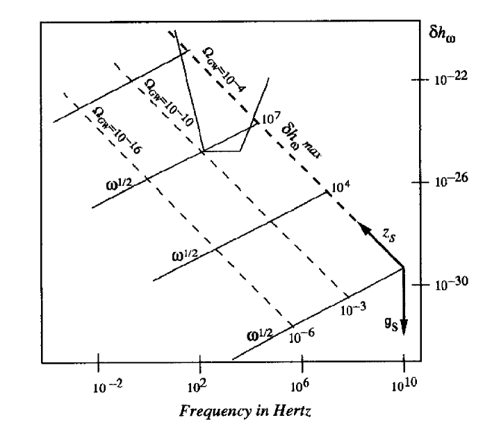
  Figure 3: GW spectra from string cosmology against interferometric sensitivity.

  which holds for scales crossing the horizon during the dilatonic era (the rest of the spectrum, which is more model-dependent, is not shown). The odd-shaped region in Fig. 3 shows the expected sensitivity of the so-called “Advanced LIGO” project³¹⁾. Resonant bars³²⁾ might also be able to reach comparable sensitivity in the kHz region, while microwave cavities, if conveniently developed, could be used in the region $10^{6}$-$10^{9}$ Hz ³³⁾. Another interesting possibility is coincidence experiments between an interferometer and a bar. The quoted sensitivity³⁴⁾ to a stochastic background, as a function of the frequency $f$, of the individual sensitivities of the bar and of the interferometer $\delta h$, and of the observation time $T_{obs}$, is:

  $$\delta\Omega_{GW}=1.5~{}10^{-5}(f/10^{3}{\rm Hz})^{3}(10^{21}\delta h_{int})(10^{21}\delta h_{bar})(T_{obs}/10^{7}~{}{\rm s})^{-1/2}.$$ (4.14)

  Obviously, detecting a stochastic backgound like ours is a formidable challenge. Also, the physical range of our parameters $g_{s},z_{s}$ could be such that no observable signal will be produced. What is perhaps more interesting is the fact that there are cosmological models that predict a non-negligible yield of GW in a range of frequencies where other sources predict just a “desert”. We hope that this will encourage experimentalists to develop suitable techniques to reach sensitivities better than $\delta h=10^{-24}$ in the $10^{6}$-$10^{9}~{}{\rm Hz}$ region.

• Can large enough seeds be produced for the generation of observed galactic (and extragalactic) magnetic fields?

  As already mentioned, seeds for generating the galactic magnetic fields through the so-called cosmic dynamo mechanism³⁵⁾ can be generated in our scenario by the amplification of the quantum fluctuations of the EM field. In this case the canonical variable is just the (Fourier transform of the) usual $A_{\mu}$ potential. In analogy with (4.11) its amplification, while outside the horizon, is described by the asymptotic solution:

  $$A_{k}\sim g^{-1}\left[C_{k}+D_{k}\int_{\eta_{ex}}^{\eta}~{}d\eta^{\prime}g^{2}(\eta^{\prime})\right]~{},$$ (4.15)

  which leads^36),37) to an overall amplification of the electromagnetic field by a factor $|c_{k}|^{2}\sim(g_{re}/g_{ex})^{2}$. Again, the main contribution to the amplification comes from the second term on the r.h.s. of eq. (4.15). One can express this result in terms of the fraction of electromagnetic energy stored in a unit of logarithmic interval of $\omega$ normalized to the one in the CMB, $\rho_{\gamma}$. One finds:

  $$r(\omega)=\frac{\omega}{\rho_{\gamma}}\frac{d\rho_{B}}{d\omega}\simeq\frac{\omega^{4}}{\rho_{\gamma}}|c_{-}(\omega)|^{2}\equiv\frac{\omega^{4}}{\rho_{\gamma}}(g_{re}/g_{ex})^{2}~{}.$$ (4.16)

  The ratio $r(\omega)$ stays constant during the phase of matter-dominated as well as radiation-dominated evolution, in which the Universe behaves like a good electromagnetic conductor³⁸⁾. In terms of $r(\omega)$ the condition that has to be satisfied in order to seed in the galaxies a magnetic field big enough to be amplified by the ordinary mechanisms of plasma physics is³⁸⁾

  $$r(\omega_{G})\geq 10^{-34}$$ (4.17)

  where $\omega_{G}\simeq(1$ Mpc$)^{-1}\simeq 10^{-14}$ Hz is the galactic scale. Using the known value of $\rho_{\gamma}$, we thus find, from (4.16, 4.17):

  $$g_{ex}<10^{-33}~{},$$ (4.18)

  i.e. a very tiny coupling at the time of exit of the galactic scale.

  The conclusion is that string (or more generally dilaton-driven) inflation stands a unique chance of explaining the origin of the galactic magnetic fields. Indeed, if the seeds of the magnetic fields are to be attributed to the amplification of vacuum fluctuations, their present magnitude can be interpreted as evidence that the fine structure constant has evolved to its present value from a tiny one during inflation.

• Can scalar, tensor (and possibly EM) perturbations explain the large-scale anisotropy of the CMB observed by COBE?

  The answer here is certainly negative as far as scalar and tensor perturbations are concerned. The reason is simple: for spectra that are normalized to $O(1)$ (at most) at the maximal amplified frequency $\omega_{1}\sim 10^{11}$ Hz, and that grow like $\omega^{1/2}$, one cannot have any substantial power at the scales $O(10^{-18}$Hz) to which COBE is sensitive. The origin of $\Delta T/T$ at large scale would have to be attributed to other effects (e.g. topological defects).

  There is however a (small?) chance³⁹⁾ that the EM perturbations themselves might explain the anisotropies of the CMB since the spectrum of electromagnetic perturbations turns out to be flatter (and more model-dependent) than that of metric perturbations. Assuming that this is the case, an interesting relation is obtained³⁹⁾ between the magnitute of large scale anysotropies and the slope of the power spectrum. Such a relation turns out to be fully consistent, with present bounds on the spectral index.

• Do all these perturbations have anything to do with the CMB itself?

  Stated differently, this is the question of how to arrive at the hot big bang of the SCM starting from our “cold” initial conditions. The reason why a hot universe can emerge at the end of our inflationary epochs (phases I and II) goes back to an idea of L. Parker⁴⁰⁾, according to which amplified quantum flluctuations can give origin to the CMB itself if Planckian scales are reached.

  Rephrasing Parker’s idea in our context amounts to solving the following bootstrap-like condition: at which moment, if any, will the energy stored in the perturbations reach the critical density?

  The total energy density $\rho_{qf}$ stored in the amplified vacuum quantum fluctuations is given by:

  $$\rho_{qf}\sim N_{eff}~{}{M_{s}^{4}\over 4\pi^{2}}\left(a_{1}/a\right)^{4}~{},$$ (4.19)

  where $N_{eff}$ is the number of effective (relativistic) species, which get produced (whose energy density decreases like $a^{-4}$) and $a_{1}$ is the scale factor at the (supposed) moment of branch-change. The critical density (in the same units) is given by:

  $$\rho_{cr}=e^{-\phi}M_{s}^{2}H^{2}~{}.$$ (4.20)

  At the beginning, with $e^{\phi}\ll 1$, $\rho_{qf}\ll\rho_{cr}$ but, in the $(-)$ branch solution, $\rho_{cr}$ decreases faster than $\rho_{qf}$ so that, at some moment, $\rho_{qf}$ will become the dominant sort of energy while the dilaton kinetic term will become negligible. It would be interesting to find out what sort of initial temperatures for the radiation era will come out of this assumption.

5 Conclusions

I want to conclude by listing which are, in my opinion, the pluses and minuses of the scenario I have advocated:

The Goodies

• Inflation comes naturally, without ad-hoc fields and fine-tuning: there is even an underlying symmetry yielding inflationary solutions.

• Initial conditions are natural, yet a simple universe would evolve into a rich and complex one.

• The kinematical problems of the SCM are solved.

• Perturbations do not grow too fast to spoil homogeneity.

• An interesting characteristic spectrum of GW is generated.

• Larger-than-usual electromagnetic perturbations are easily generated and could explain the galactic magnetic fields.

• A hot big bang could be a natural outcome of our inflationary scenario.

The Baddies

• A scale-invariant spectrum is all but automatic (unlike what happens in normal vacuum-energy-driven inflation).

• Our understanding of the high curvature (stringy) phase and of the (crucial and necessary) change of branch is still poorly understood (in spite of recent progress in Conformal Field Theory).

On the whole this does not look like a bad score for a four-year-old kid!

Acknowledgements

I would like to acknowledge the help and encouragement of my collaborators in the work reported here: Ramy Brustein (CERN–Beer Sheva), Maurizio Gasperini (Turin), Massimo Giovannini (CERN–Turin), and Slava Mukhanov (Zurich–Moscow). This work has also benefited from earlier collaborations with Jnan Maharana (Bhubaneswar), Kris Meissner (Trieste–Varsaw), Roberto Ricci (CERN–Rome), Norma Sanchez (Paris) and Nguyen Suan Han (Hanoi).

References

- [1] S. Weinberg, Gravitation and Cosmology, John Wiley & Sons, Inc., New York (1972).
- [2] G. Smoot et al., Astrophys. J. 396 (1992) L1.
- [3] L.F. Abbott and So-Young Pi (eds.), Inflationary Cosmology, World Scientific, Singapore (1986).
- [4] E. Kolb and M. Turner, The Early Universe, Addison-Wesley, New York (1990).
- [5] G. Veneziano, Europhys. Lett. 2 (1986) 133.
- [6] G. Veneziano, “Quantum strings and the constants of Nature”, in The Challenging Questions (Erice, 1989), ed. A. Zichichi, Plenum Press, New York (1990).
-
[7]
C. Lovelace, Phys. Lett. B135 (1984) 75;
C.G. Callan, D. Friedan, E.J. Martinec and M.J. Perry, Nucl. Phys. B262 (1985) 593. - [8] E.S. Fradkin and A.A. Tseytlin, Nucl. Phys. B261 (1985) 1.
-
[9]
P. Jordan, Z. Phys. 157 (1959) 112;
C. Brans and R.H. Dicke, Phys. Rev. 124 (1961) 925. - [10] E. Witten, Phys. Lett. B149 (1984) 351.
- [11] T.R. Taylor and G. Veneziano, Phys. Lett. B213 (1988) 459.
- [12] See, for instance, E. Fischbach and C. Talmadge, Nature 356 (1992) 207.
- [13] J. Ellis et al., Phys. Lett. B228 (1989) 264.
- [14] T. Damour and A. M. Polyakov, Nucl. Phys. B423 (1994) 532.
- [15] G. Veneziano, Phys. Lett. B265 (1991) 287; Proceeding 4th PASCOS Conference (Syracuse, May 1994), K.C. Wali ed., World Scientific, Singapore, p. 453.
- [16] M. Gasperini and G. Veneziano, Astropart. Phys. 1 (1993) 317; Mod. Phys. Lett. A8 (1993) 3701; Phys. Rev. D50 (1994) 2519.
-
[17]
A.A. Tseytlin, Mod. Phys. Lett. A6 (1991) 1721;
A.A. Tseytlin and C. Vafa, Nucl. Phys. B372 (1992) 443. -
[18]
E. Kiritsis and C. Kounnas, Phys. Lett. B331 (1994) 51;
A.A. Tseytlin, Phys. Lett. B334 (1994) 315. -
[19]
P. Aspinwall, B. Greene and D. Morrison, Phys. Lett. B303 (1993) 249;
E. Witten, Nucl. Phys. B403 (1993) 159. - [20] R. Brustein and G. Veneziano, Phys. Lett. B329 (1994) 429.
- [21] N. Kaloper, R. Madden and K. A. Olive, Towards a singularity-free inflationary universe?, Univ. Minnesota preprint UMN-TH-1333/95 (June 1995).
- [22] J. Levin and K. Freese, Nucl. Phys. B421 (1994) 635.
-
[23]
L.P. Grishchuk, Sov. Phys. JEPT 40 (1975)
409;
A.A. Starobinski, JEPT Lett. 30 (1979) 682;
V.A. Rubakov, M. Sazhin and A. Veryaskin, Phys. Lett. B115 (1982) 189;
R. Fabbri and M. Pollock, Phys. Lett. B125 (1983) 445. - [24] M. Gasperini, Amplification of vacuum fluctuations in string cosmology backgrounds, these proceedings.
-
[25]
M. Gasperini, N. Sanchez and G. Veneziano,
Int. J. Theor. Phys. A6
(1991) 3853;
Nucl. Phys. B364 (1991) 365;
M. Gasperini, Phys. Lett. B258 (1991) 70;
G. Veneziano, Helv. Phys. Acta 64 (1991) 877. - [26] See, e.g. V. Mukhanov, H.A. Feldman and R. Brandenberger, Phys. Rep. 215 (1992) 203.
- [27] R.B. Abbot, B. Bednarz and S.D. Ellis, Phys. Rev. D33 (1986) 2147.
- [28] R. Brustein, M. Gasperini, M. Giovannini, V. Mukhanov and G. Veneziano, Phys. Rev. D51 (1995) 6744.
-
[29]
G. F. R. Ellis and M. Bruni,
Phys. Rev. D40 (1989) 1804;
M. Bruni, G. F. R. Ellis and P. K. S. Dunsby, Class. Quant. Grav. 9 (1992) 921. -
[30]
R. Brustein, M. Gasperini, M. Giovannini
and G. Veneziano, Relic gravitational waves from
string cosmology, CERN-TH/95-144 (1995), Phys. Lett. in press;
see also M. Gasperini and M. Giovannini, Phys. Rev. D47 (1992) 1529. -
[31]
R.E. Vogt et al., Laser Interferometer
Gravitational-Wave Observatory,
proposal to the National Science Foundation (Caltech, 1989);
C. Bradascia et al., in Gravitational Astronomy, eds. D.E. McClelland and H. Bachor, World Scientific, Singapore, (1991). -
[32]
G. V. Pallottino and V. Pizzella, Nuovo Cim.
C4 (1981) 237;
M. Cerdonio et. al, Phys. Rev. Lett. 71 (1993) 4107. -
[33]
F. Pegoraro, E. Picasso and L. Radicati,
J. Phys. A11 (1978) 1949;
C. M. Caves, Phys. Lett. B80 (1979) 323;
C. E. Reece et al., Phys. Lett. A104 (1984) 341. - [34] P. Astone, J. A. Lobo and B. F. Schutz, Class. Quant. Grav. 11 (1994) 2093.
-
[35]
E. N. Parker, Cosmical Magnetic Fields,
Clarendon, Oxford (1979);
Y. B. Zeldovich, A. A. Ruzmaikin and D. D. Sokoloff, Magnetic fields in astrophysics, Gordon and Breach, New York (1983). - [36] M. Gasperini, M. Giovannini and G. Veneziano, Primordial magnetic fields from string cosmology, CERN-TH/95-85 (April 1995).
- [37] D. Lemoine and M. Lemoine, Primordial magnetic fields in string cosmology, Inst. d’Astrophysique de Paris preprint (April 1995).
- [38] M. S. Turner and L. M. Widrow, Phys. Rev. D37 (1988) 2743.
- [39] M. Gasperini, M. Giovannini and G. Veneziano, Electromagnetic origin of the CMB anisotropy in string cosmology, CERN-TH/95-102 (April 1995).
- [40] L. Parker, Nature 261 (1976) 20.